Information width

Abstract

Kolmogorov argued that the concept of information exists also in problems with no underlying stochastic model (as Shannon’s information representation) for instance, the information contained in an algorithm or in the genome. He introduced a combinatorial notion of entropy and information $I(x:\mathsf{y})$ conveyed by a binary string $x$ about the unknown value of a variable $\mathsf{y}$. The current paper poses the following questions: what is the relationship between the information conveyed by $x$ about $\mathsf{y}$ to the description complexity of $x$ ? is there a notion of cost of information ? are there limits on how efficient $x$ conveys information ? To answer these questions Kolmogorov’s definition is extended and a new concept termed information width which is similar to $n$-widths in approximation theory is introduced. Information of any input source, e.g., sample-based, general side-information or a hybrid of both can be evaluated by a single common formula. An application to the space of binary functions is considered.

Keywords: Binary functions, Combinatorics, $n$-widths, VC-dimension

1 Introduction

Kolmogorov [13] sought for a measure of information of ‘finite objects’. He considered three approaches, the so-called combinatorial, probabilistic and algorithmic. The probabilistic approach corresponds to the well-established definition of the Shannon entropy which applies to stochastic settings where an ‘object’ is represented by a random variable. In this setting, the entropy of an object and the information conveyed by one object about another are well defined. Here it is necessary to view an object (or a finite binary string) as a realization of a stochastic process. While this has often been used, for instance, to measure the information of English texts [7, 14] by assuming some finite-order Markov process, it is not obvious that such modeling of finite objects provides a natural and a universal representation of information as Kolmogorov states in [13]: What real meaning is there, for example, in asking how much information is contained in (the book) ”War and Peace” ? Is it reasonable to … postulate some probability distribution for this set ? Or, on the other hand, must we assume that the individual scenes in this book form a random sequence with stochastic relations that damp out quite rapidly over a distance of several pages ? These questions led Kolmogorov to introduce an alternate non-probabilistic and algorithmic notion of the information contained in a finite binary string. He defined it as the length of the minimal-size program that can compute the string. This has been later developed into the so-called Kolmogorov Complexity field [15].

In the combinatorial approach, Kolmogorov investigated another non stochastic measure of information for an object $y$. Here $y$ is taken to be any element in a finite space $\mathbb{Y}$ of objects. In [13] he defines the ‘entropy’ of $\mathbb{Y}$ as $H(\mathbb{Y})=\log|\mathbb{Y}|$ where $|\mathbb{Y}|$ denotes the cardinality of $\mathbb{Y}$ and all logarithms henceforth are taken with respect to $2$. As he writes, if the value of $\mathbb{Y}$ is known to be $\mathbb{Y}=\{y\}$ then this much entropy is ‘eliminated’ by providing $\log|\mathbb{Y}|$ bits of ‘information’.

Let $R=\mathbb{X}\times\mathbb{Y}$ be a general finite domain and consider a set

$$A\subseteq R$$ (1)

that consists of all ‘allowed’ values of pairs $(x,y)\in R$. The entropy of $\mathbb{Y}$ is defined as

$$H(\mathbb{Y})=\log|\Pi_{\mathbb{Y}}(A)|$$

where $\Pi_{\mathbb{Y}}(A)\equiv\{y\in\mathbb{Y}:(x,y)\in A\text{ for some }x\in\mathbb{X}\}$ denotes the projection of $A$ on $\mathbb{Y}$. Consider the restriction of $A$ on $\mathbb{Y}$ based on $x$ which is defined as

$$Y_{x}=\{y\in\mathbb{Y}:(x,y)\in A\},\;x\in\Pi_{\mathbb{X}}(A)$$ (2)

then the conditional combinatorial entropy of $\mathbb{Y}$ given $x$ is defined as

$$H(\mathbb{Y}|x)=\log|Y_{x}|.$$ (3)

Kolmogorov defines the information conveyed by $x$ about $\mathbb{Y}$ by the quantity

$$I(x:\mathbb{Y})=H(\mathbb{Y})-H(\mathbb{Y}|x).$$ (4)

Alternatively, we may view $I(x:\mathbb{Y})$ as the information that a set $Y_{x}$ conveys about another set $\mathbb{Y}$ satisfying $Y_{x}\subseteq\mathbb{Y}$. In this case we let the domain be $R=\Pi_{\mathbb{Y}}(A)\times\Pi_{\mathbb{Y}}(A)$, $A_{x}\subseteq R$ is the set of permissible pairs $A_{x}=\{(y,y^{\prime}):y\in\Pi_{\mathbb{Y}}(A),y^{\prime}\in Y_{x}\}$ and the information is defined as

$$I(Y_{x}:\mathbb{Y})=\log|\Pi_{\mathbb{Y}}(A)|^{2}-\log(|Y_{x}||\Pi_{\mathbb{Y}}(A)|).$$ (5)

We will refer to this representation as Kolmogorov’s information between sets. Clearly, $I(Y_{x}:\mathbb{Y})=I(x:\mathbb{Y})$.

In many applications, knowing an input $x$ only conveys partial information about an unknown value $y\in\mathbb{Y}$. For instance, in problems which involve the analysis of algorithms on discrete classes of structures, such as sets of binary vectors or functions on a finite domain, an algorithmic search is made for some optimal element in this set based only on partial information. One such paradigm is the area of statistical pattern recognition [26, 2] where an unknown target, i.e., a pattern classifier, is seeked based on the information contained in a finite sample and some side-information. This information is implicit in the particular set of classifiers that form the possible hypotheses.

For example, let $n$ be a positive integer and consider the domain $[n]=\{1,\ldots,n\}$. Let $F=\{0,1\}^{[n]}$ be the set of all binary functions $f:[n]\rightarrow\{0,1\}$. The power set ${\mathcal{P}}(F)$ represents the family of all sets $G\subseteq F$. Repeating this, we have ${\mathcal{P}}({\mathcal{P}}(F))$ as the collection of all properties of sets $G$, i.e., a property is a set whose elements are subsets $G$ of $F$. We denote by ${\mathcal{M}}$ a property of a set $G$ and write $G\models{\mathcal{M}}$. Suppose that we seek to know an unknown target function $t\in F$. Any partial information about $t$ which may be expressed by $t\in G\models{\mathcal{M}}$ can effectively reduce the search space. It has been a long-standing problem to try to quantify the value of general side-information for learning (see [24] and references therein).

We assert that Kolmogorov’s combinatorial framework may serve as a basis. We let $x$ index possible properties ${\mathcal{M}}$ of subsets $G\subseteq F$ and the object $y$ represent the unknown target $t$ which may be any element of $F$. Side information is then represented by knowing certain properties of sets that contain the target. The input $x$ conveys that $t$ is in some subset $G$ that has a certain property ${\mathcal{M}}_{x}$.

In principle, Kolmogorov’s quantity $I(x:\mathbb{Y})$ should serve as the value of information in $x$ about the unknown value of $y$. However, its current form (4) is not general enough since it requires that the target $y$ be restricted to a fixed set $Y_{x}$ on knowledge of $x$. To see this, suppose $t$ is in a set that satisfies property ${\mathcal{M}}_{x}$. Consider the collection $\{G_{z}\}_{z\in Z_{x}}$ of all subsets $G_{z}\subseteq F$ that have this property. Clearly, $t\in\bigcup_{z\in Z_{x}}G_{z}$ hence we may first consider $Y_{x}=\bigcup_{z\in Z_{x}}G_{z}$ but some useful information implicit in this collection is ignored as we now show: consider two properties ${\mathcal{M}}_{0}$ and ${\mathcal{M}}_{1}$ with corresponding index sets $Z_{x_{0}}$ and $Z_{x_{1}}$ such that $\bigcup_{z\in Z_{x_{0}}}G_{z}=\bigcup_{z\in Z_{x_{1}}}G_{z}\equiv F^{\prime}\subseteq F$. Suppose that most of the sets $G_{z}$, $z\in Z_{x_{0}}$ are small while the sets $G_{z}$, $z\in Z_{x_{1}}$ are large. Clearly, property ${\mathcal{M}}_{0}$ is more informative than ${\mathcal{M}}_{1}$ since starting with knowledge that $t$ is in a set that satisfies it should take (on average) less additional information (once the particular set $G$ becomes known) in order to completely specify $t$. If, as above, we let $A_{x_{0}}=\bigcup_{z\in Z_{x_{0}}}G_{z}$ and $A_{x_{1}}=\bigcup_{z\in Z_{x_{1}}}G_{z}$ then we have $I(x_{0}:\mathbb{Y})=I(x_{1}:\mathbb{Y})$ which wrongly implies that both properties are equally informative. Knowing ${\mathcal{M}}_{0}$ provides implicit information associated with the collection of possible sets $G_{z}$, $z\in Z_{x_{0}}$. This implicit structural information cannot be represented in (4).

2 Overview

In [23] we began to consider an extension of Kolmogorov’s combinatorial information that can be to applied for more general settings. The current paper further builds upon this and continues to explore the ‘objectification’ of information, viewing it as a ‘static’ relationship between sets of objects in contrast to the standard Shannon representation. As it is based on basic set theoretic principles no assumption is necessary concerning the underlying space of objects other than its finiteness. It is thus more fundamental than the standard probability-based representation used in information theory. It is also more general than Bayesian approaches, for instance in statistical pattern recognition, which assume that a target $y$ is randomly drawn from $\mathbb{Y}$ according to a prior probability distribution.

The main two contributions of the paper are, first, the introduction of a set-theoretic framework of information and its efficiency, and secondly the application of this framework to classes of binary functions. Specifically, in Section 6 we define a quantity called the information width (Definition 6) which measures the information conveyed about an unknown target $y$ by a maximally-informative input of a fixed description complexity $l$ (this notion is defined in Definition 9). The first result, Theorem 1, computes this width and it is consequently used as a reference point for a comparison of the information value of different inputs. This is done via the measures of cost and efficiency of information defined in Definitions 5 and 7. The width serves as a universal reference against which any type of information input may be computed and compared, for instance, the information of a finite data sample used in a problem of learning can be compared to other kinds of side-information.

In Section 7 we apply the framework to the space of binary functions on a finite domain. We consider information which is conveyed via properties of classes of binary functions, specifically, those that relate to the complexity of learning such functions. The properties are stated in terms of combinatorial quantities such as the Vapnik-Chervonenkis (VC) dimension. Our interest in investigating the information conveyed by such properties stems from the large body of work on learning binary function classes (see for instance [17, 4, 19]). This is part of the area called statistical learning theory that deals with computing the complexity of learning over hypotheses classes, e.g., neural networks, using various algorithms each with its particular type of side information (which is sometimes referred to as the ‘inductive bias’, see [18]).

For instance it is known [2] that learning an unknown target function in a class of VC-dimension (defined in Definition 8) which is no greater than $d$ requires a training sample of size linear in $d$. The knowledge that the target is in a class which has this property conveys the useful information that there exist an algorithm which learns any target in this class to within arbitrarily low error based on a finite samples (in general this is impossible if the VC-dimension is infinite). But how valuable is this information, can it be quantified and compared to other types of side information ?

The theory developed here answers this and treats the problem of computing the value of information in a uniform manner for any source. The generality of this approach stands on its set-theoretic basis. Here information, or entropy, is defined in terms of the number of bits that it takes to index objects in general sets. This is conveniently applicable to settings such as those in learning theory where the underlying structures consist of classes of objects or inference models (hypotheses) such as binary functions (classifiers), decision trees, Boolean formulae, neural networks. Another area (unrelated to learning theory) which can be applicable is computational biology. Here a sequence of the nucleotides or amino acids make up DNA, RNA or protein molecules and one is interested in the amount of functional information needed to specify sequences with internal order or structure. Functional information is not a property of any one molecule, but of the ensemble of all possible sequences, ranked by activity. As an example, [25] considers a pile of DNA, RNA or protein molecules of all possible sequences, sorted by activity with the most active at the top. More information is required to specify molecules that carry out difficult tasks, such as high-affinity binding or the rapid catalysis of chemical reactions with high energy barriers, than is needed to specify weak binders or slow catalysts. But, as stated in [25], precisely how much more functional information is required to specify a given increase in activity is unknown. Our model may be applicable here if we let all sequences of a fixed level $\alpha$ of activity be in the same class that satisfies a property ${\mathcal{M}}_{\alpha}$. Its description complexity (introduced later) may represent the amount of functional information.

In Section 7 we consider an application of this model and state Theorems 2 – 5 which estimate the information value, the cost and the description complexity associated with different properties. This allows to compute their information efficiency and compare their relative values. For instance, Theorem 5 considers a hybrid property which consists of two sources of information, a sample of size $m$ and side-information about the VC-dimension $d$ of the class that contains the target. By computing the efficiency with respect to $m$ and $d$ we determine how effective is each of these sources. In Section 8 we compare the information efficiency of several additional properties of this kind.

3 Combinatorial formulation of information

In this section we extend the information measure (4) to one that applies to a more general setting (as discussed in Section 1) where knowledge of $x$ may still leave some vagueness about the possible value of $y$. As in [13] we seek a non-stochastic representation of the information conveyed by $x$ about $y$.

Henceforth let $\mathbb{Y}$ be a general finite domain, let $\mathbb{Z}={\mathcal{P}}(\mathbb{Y})$ and $\mathbb{X}={\mathcal{P}}(\mathbb{Z})$ where as before for a set $E$ we denote by ${\mathcal{P}}(E)$ its power set. Here $\mathbb{Z}$ represents the set of indices $z$ of all possible sets $Y_{z}\subseteq\mathbb{Y}$ and $\mathbb{X}$ is the set of indices $x$ of all possible collections, i.e., subsets $Z_{x}\subseteq\mathbb{Z}$ of indices of sets $Y_{z}$, $z\in\mathbb{Z}$. We say that a set $Y_{z}\subseteq\mathbb{Y}$ has a property ${\mathcal{M}}_{x}$ if $z\in Z_{x}$ where $Z_{x}$ is the uniquely corresponding collection of ${\mathcal{M}}_{x}$.

The previous representation based on (1) is subsumed by this representation since instead of $\mathbb{X}$ we have $\mathbb{Z}$ and the sets $Y_{x}$, $x\in\Pi_{\mathbb{X}}(A)$ defined in (2) are now represented by the sets $Y_{z}$, $z\in Z_{x}$. Since $\mathbb{X}$ indexes all possible properties of sets in $\mathbb{Y}$ then for any $A$ as in (1) there exists an $x\in\mathbb{X}$ in the new representation such that $\Pi_{\mathbb{X}}(A)$ in Kolmogorov’s representation is equivalent to $Z_{x}$ in the new representation. Therefore what was previously represented by the sets $\{Y_{x}:x\in\Pi_{\mathbb{X}}(A)\}$ is now the collection of sets $\{Y_{z}:z\in Z_{x}\}$. In this new representation a given input $x$ can point to multiple subsets $Y_{z}$ of $\mathbb{Y}$, $z\in Z_{x}$, and hence apply for the more general settings discussed in the previous section.

We will view the information conveyed by $x$ about an unknown object $y$ through two perspectives. The first is held by the side that provides the information and the second by the side which acquires it. From the side of the provider, we denote by the subset $\mathsf{y}\subset\mathbb{Y}$ a set of target values $y$, for instance, solutions to a problem any one of which the provider may wish to inform the acquirer. In general the provider provides partial information about $y$ via an object $x\in\mathbb{X}$ which is used as a means of representing this information and as input to the acquirer.

From the acquirer’s side, initially (before seeing $x$) the set of possible targets is the whole target-domain $\mathbb{Y}$ since he does not ‘know’ the subset $\mathsf{y}$. After seeing the input $x$ he then has a collection of sets $Y_{z}$, $z\in Z_{x}$, one of which is ensured (by the provider) to intersect the subset $\mathsf{y}$. In this case we say that $x$ is informative about $\mathsf{y}$ (Definition 1). Kolmogorov’s representation fits the acquirer’s perspective where the unknown subset $\mathsf{y}$ is just the whole target domain $\mathbb{Y}$ (known by default) and therefore $x$ is the only variable in the information formula of (4). In all subsequent definitions that involve $\mathsf{y}$ we may switch between the two perspectives simply by replacing $\mathsf{y}$ with $\mathbb{Y}$.

Definition 1

Let $\mathsf{y}\subseteq\mathbb{Y}$ be fixed. An input object $x\in\mathbb{X}$ is called informative for $\mathsf{y}$, denoted $x\vdash\mathsf{y}$, if there exists a $z\in Z_{x}$ with a corresponding set $Y_{z}$ such that $\mathsf{y}\bigcap Y_{z}\neq\emptyset$.

The following is our definition of the combinatorial value of information.

Definition 2

Let $\mathsf{y}\subseteq\mathbb{Y}$ and consider any $x\in\mathbb{X}$ such that $x\vdash\mathsf{y}$. Define by

$$I(z:\mathsf{y})=\log(|\mathsf{y}\bigcup Y_{z}|^{2})-\log(|\mathsf{y}||Y_{z}|).$$

Then the information conveyed by $x$ about the unknown value $y\in\mathsf{y}$ is defined as

$$I(x:\mathsf{y})\equiv\frac{1}{|Z_{x}|}\sum_{z\in Z_{x}}I(z:\mathsf{y}).$$

Remark 1

For a fixed $x$, the information value $I(x:\mathsf{y})$ is in general dependent on $\mathsf{y}$ since different $\mathsf{y}$ for which $x$ is informative ($x\vdash\mathsf{y}$) may have different values of $I(z:\mathsf{y})$, $z\in Z_{x}$. The information value is non-negative real measured in bits.

Henceforth, it will be convenient to assume that $I(x:\mathsf{y})=0$ whenever $x$ is not informative for $\mathsf{y}$.

Remark 2

We will refer to $I(x:\mathsf{y})$ as the provider’s (or provided) information about the unknown target $y$ given $x$. The acquirer’s (or acquired) information is defined based on the special case where $\mathsf{y}=\mathbb{Y}$. Here we have $|\mathsf{y}\bigcup Y_{z}|=|\mathbb{Y}\bigcup Y_{z}|=|\mathbb{Y}|$ and the information value becomes

$$I(x:\mathbb{Y}) = \frac{1}{|Z_{x}|}\sum_{z\in Z_{x}}\left[2\log|\mathbb{Y}|-\log|\mathbb{Y}|-\log|Y_{z}|\right]$$ (6)

$$= \log|\mathbb{Y}|-\frac{1}{|Z_{x}|}\sum_{z\in Z_{x}}\log|Y_{z}|.$$

Definition 2 is consistent with (4) in that the representation of uncertainty is done as in [13] in a set-theoretic approach since all expressions in (6) involve set-quantities such as cardinalities and restrictions of sets. The expression of (4) is a special case of (6) with $Z_{x}$ being a singleton set and $\mathsf{y}=\mathbb{Y}$. In defining $I(z:\mathsf{y})$ we have implicitly extended Kolmogorov’s information $I(Y_{x}:\mathbb{Y})$ between sets $Y_{x}$ and $\mathbb{Y}$ that satisfy $Y_{x}\subseteq\mathbb{Y}$ (see (5)) into the more general definition where one of the two sets is not necessarily contained in the other and neither one equals the whole space $\mathbb{Y}$, i.e., $I(z:\mathsf{y})\equiv I(Y_{z}:\mathsf{y})$ is the information between the sets $Y_{z}$ and $\mathsf{y}$ where $Y_{z}$ is not necessarily contained in $\mathsf{y}$. Here we take the underlying two-dimensional domain as $R=(\mathsf{y}\bigcup Y_{z})\times(\mathsf{y}\bigcup Y_{z})$ and the set of permissible pairs as

$$A_{z,\mathsf{y}}=\{(y,y^{\prime}):y\in\mathsf{y},y^{\prime}\in Y_{z}\}\subset R.$$

We may view the relationship between the provider and acquirer as a transformation between sets

$$\mathsf{y}\rightarrow\{Y_{z}:z\in Z_{x}\}{\rightarrow}\mathbb{Y}$$

where the provider, knowing the set $\mathsf{y}$, chooses some $x$ with which he represents the unknown value of $y$ and for him, the amount of information remaining about $y$ as conveyed by $x$ is $I(x:\mathsf{y})$ bits. The acquirer, starting from knowing only $\mathbb{Y}$, uses $x$, or equivalently the corresponding collection of sets $\{Y_{z}:z\in Z_{x}\}$, as an intermediate ‘medium’ to acquire $I(x:\mathbb{Y})$ bits of information about the unknown value of $y$. Note that, in general, the provider’s information may be smaller, equal or larger than the acquired information. For instance, fix an $x$, then directly from Definition 2 for any $z\in Z_{x}$ we can compare $I(z:\mathsf{y})$ versus $I(z:\mathbb{Y})$ and see that if $|\mathsf{y}\bigcup Y_{z}|$ is closer to $|\mathbb{Y}|$ (or $|\mathsf{y}|$) than to $|\mathsf{y}|$ (or $|\mathbb{Y}|$) then $I(z:\mathsf{y})>I(z:\mathbb{Y})$ (or $I(z:\mathbb{Y})>I(z:\mathsf{y})$) respectively. Thus taking the average over all $z\in Z_{x}$ it is possible in general to have $I(x:\mathsf{y})$ smaller, larger or equal to $I(x:\mathbb{Y})$.

In this paper we will primarily use the acquirer’s perspective and will thus refer to the sum in (6) as the conditional combinatorial entropy which is defined next.

Definition 3

Let

$$H(\mathbb{Y}|x)\equiv\frac{1}{|Z_{x}|}\sum_{z\in Z_{x}}\log|Y_{z}|$$ (7)

be the conditional entropy of $\mathbb{Y}$ given $x$.

It will be convenient to express the conditional entropy as

$$H(\mathbb{Y}|x)=\sum_{k\geq 2}\omega_{x}(k)\log k$$

with

$$\omega_{x}(k)=\frac{|\{z\in Z_{x}:|Y_{z}|=k\}|}{|Z_{x}|}.$$ (8)

We will refer to this quantity $\omega_{x}(k)$ as the conditional density function of $k$. The factor of $\log k$ comes from $\log|Y_{z}|$ which from (3) is the combinatorial conditional-entropy $H(\mathbb{Y}|z)$.

4 Description complexity

We have so far defined the notion of information $I(x:\mathsf{y})$ about the unknown value $y$ conveyed by $x$. Let us now define the description complexity of $x$.

Definition 4

The description complexity of $x$, denoted $\ell(x)$, is defined as

$$\ell(x)\equiv\log\frac{|\mathbb{Z}|}{|Z_{x}|}.$$ (9)

Remark 3

The description complexity $\ell(x)$ is a positive real number measured in bits. It takes a fractional value if the cardinality of $Z_{x}$ is greater than half that of $\mathbb{Z}$.

Definition 4 is motivated from the following: from Section 3, the input $x$ conveys a certain property common to every set $Y_{z}$, $z\in Z_{x}\subseteq\mathbb{Z}$, such that the unknown value $y$ is an element of at least one such set $Y_{z}$. Without the knowledge of $x$ these indices $z$ are only known to be elements of $\mathbb{Z}$ in which case it takes $\log|\mathbb{Z}|$ bits to describe any $z$, or equivalently, any $Y_{z}$. If $x$ is given then the length of the binary string that describes a $z$ in $Z_{x}$ is only $\log|Z_{x}|$. The set $Z_{x}$ can therefore be described by a string of length $\log|\mathbb{Z}|-\log|Z_{x}|$ which is precisely the right side of (9). Alternatively, $\ell(x)$ is the information $I(x:\mathbb{Z})$ gained about the unknown value $z$ given $x$ (since $x$ points to a single set $Z_{x}$ then this information follows directly from Kolmogorov’s formula (4)).

As $|Z_{x}|$ decreases there are fewer possible sets $Y_{z}$ that satisfy the property described by $x$ and the description complexity $\ell(x)$ increases. In this case, $x$ conveys a more ‘special’ property of the possible sets $Y_{z}$ and the ‘price’ of describing such a property increases. The following is a useful result.

Lemma 1

Denote by $Z^{c}_{x}=\mathbb{Z}\setminus Z_{x}$ the complement of the set $Z_{x}$ and let $x^{c}$ denote the input corresponding to $Z^{c}_{x}$. Then

$$\ell(x^{c})=-\log(1-2^{-\ell(x)}).$$

Proof: Denote by $p=|Z_{x}|/|\mathbb{Z}|$. Then by definition of the description complexity we have $\ell(x^{c})=-\log(1-p).$ Clearly,

$$2^{-\log\frac{1}{1-p}}=1-2^{-\log\frac{1}{p}}$$

from which the result follows. $\square$

Remark 4

Since clearly the proportion of elements $z\in\mathbb{Z}$ which are in $Z_{x}$ plus the proportion of those in $Z^{c}_{x}$ is fixed and equals $1$ then $2^{-\ell(x)}+2^{-\ell(x^{c})}=1$. If the description complexity $\ell(x)$ and $\ell(x^{c})$ change (for instance with respect to an increase in $|\mathbb{Z}|$) then they change in opposite directions. However, the cardinalities of the corresponding sets $Z_{x}$ and $Z^{c}_{x}$ may both increase (9) for instance if $|\mathbb{Z}|$ grows at a rate faster than the rate of change of either $\ell(x)$ or $\ell(x^{c})$.

A question to raise at this point is whether the following trivial relationship between $\ell(x)$ and the entropy $H(\mathbb{Y}|x)$ holds,

$$\ell(x)+H(\mathbb{Y}|x)\stackrel{{\scriptstyle?}}{{=}}H(\mathbb{Y}).$$ (10)

This is equivalent to asking if

$$\ell(x)\stackrel{{\scriptstyle?}}{{=}}I(x:\mathbb{Y})$$ (11)

or in words, does the price of describing an input $x$ equals the information gained by knowing it ?

As we show next, the answer depends on certain characteristics of the set $Z_{x}$. When (4) does not apply but (6) does, then in general, the relation does not hold.

5 Scenario examples

In all the following scenarios we take the acquirer’s perspective, i.e., with no input given the unknown $y$ is only known to be in $\mathbb{Y}$. As the first scenario, we start with the simplest uniform setting which is defined as follows:

Scenario S1: As in (2)-(4), an input $x$ amounts to a single set $Y_{x}$. The set $Z_{x}$ is a singleton $\{Y_{x}\}$ so $|Z_{x}|=1$ and instead of $\mathbb{Z}$ we have $\Pi_{\mathbb{X}}(A)$. We impose the following conditions: for all $x,x^{\prime}\in\mathbb{X}$, $Y_{x}\bigcap Y_{x^{\prime}}=\emptyset$, $|Y_{x}|=|Y_{x^{\prime}}|$. With $\mathbb{Y}=\bigcup_{x\in\mathbb{X}}Y_{x}$ then it follows that for any $x$, $|Y_{x}|=\frac{|\mathbb{Y}|}{|\mathbb{X}|}$. From (4) it follows that the description complexity of any $x$ is

$$\ell(x)=\log\frac{|\mathbb{X}|}{1}=\log|\mathbb{X}|$$

and the entropy

$$H(\mathbb{Y}|x)=\log|Y_{x}|=\log\left(\frac{|\mathbb{Y}|}{|\mathbb{X}|}\right).$$

We therefore have

$$\ell(x)+H(\mathbb{Y}|x)=\log|\mathbb{X}|+\log|\mathbb{Y}|-\log|\mathbb{X}|=\log|\mathbb{Y}|.$$

Since the right side equals $H(\mathbb{Y})$ then (10) holds. Next consider another scenario:

Scenario S2: An input $x$ gives a single set $Y_{x}$ but now for any two distinct $x,x^{\prime}$, we only force the condition that $|Y_{x}|=|Y_{x^{\prime}}|$, i.e., the intersection $Y_{x}\bigcap Y_{x^{\prime}}$ may be non-empty. The description complexity $\ell(x)$ is the same as in the previous scenario and for any $x,x^{\prime}\in\mathbb{X}$ the entropy is the same $H(\mathbb{Y}|x)=H(\mathbb{Y}|x^{\prime})$ with a value of $\log\left(\frac{\alpha|\mathbb{Y}|}{|\mathbb{X}|}\right)$, for some $\alpha\geq 1$. So

$$\ell(x)+H(\mathbb{Y}|x)=\log|\mathbb{X}|+\log\left(\frac{\alpha|\mathbb{Y}|}{|\mathbb{X}|}\right)=\log\left(\alpha|\mathbb{Y}|\right)\geq\log|\mathbb{Y}|.$$

Hence the left side of (10) is greater than or equal to the right side. By (11), this means that the ‘price’, i.e., the description complexity per bit of information may be larger than $1$.

Let us introduce at this point the following combinatorial quantity:

Definition 5

The cost of information $I(x:\mathsf{y})$, denoted $\kappa_{\mathsf{y}}(x)$, is defined as

$$\kappa_{\mathsf{y}}(x)=\frac{\ell(x)}{I(x:\mathsf{y})}$$

and represents the number of description bits of $x$ per bit of information about the unknown value of $y$ as conveyed by $x$.

Thus, letting $\mathsf{y}=\mathbb{Y}$ and considering the two previous scenarios where Kolmogorov’s definition (4) applies then the cost of information equals $1$ or at least $1$, respectively. As the next scenario, let us consider the following:

Scenario S3: We follow the setting of Definition 2 where an input $x$ means that the unknown value of $y$ is contained in at least one set $Y_{z}$, $z\in Z_{x}$ hence $|Z_{x}|\geq 1$. Suppose that $\frac{|\mathbb{Y}|}{|\mathbb{X}|}\equiv a$ for some integer $a\geq 1$ and assume that for all $x\in\mathbb{X}$, $H(\mathbb{Y}|x)=\log(a)$. (The sets $Y_{z}$, $z\in Z_{x}$ may still differ in size and overlap). Thus we have

$$\ell(x)+H(\mathbb{Y}|x)=\log\frac{|\mathbb{Z}|}{|Z_{x}|}+\log\frac{|\mathbb{Y}|}{|\mathbb{X}|}.$$ (12)

Suppose that $\frac{|\mathbb{Z}|}{|\mathbb{X}|}\equiv b$ for some integer $b\geq 1$, $Z_{x}\bigcap Z_{x^{\prime}}=\emptyset$ and $|Z_{x}|=|Z_{x^{\prime}}|$ for any $x,x^{\prime}\in\mathbb{X}$. Since $\mathbb{Z}=\bigcup_{x\in\mathbb{X}}Z_{x}$ then $|Z_{x}|=b$ for all $x\in\mathbb{X}$. The right side of (12) equals $\log|\mathbb{Y}|$ and (10) is satisfied. If for some $x,x^{\prime}$ we have $|Z_{x}|<b$ and $|Z_{x^{\prime}}|>b$ (with entropies both still at $\log(a)$) then the left side of (10) is greater than or less than $H(\mathbb{Y})$, respectively. Hence it is possible in this scenario for the cost $\kappa_{\mathsf{y}}(x)$ to be greater or less than $1$. To understand why for some inputs $x$ the cost may be strictly smaller than $1$ observe that under the current scenario the actual set $Y_{z}$ which contains the unknown $y$ remains unknown even after producing the description $x$. Thus in this case the left side of (10) represents the total description complexity of the unknown value of $y$ (on average over all possible sets $Y_{z}$) given that the only fact known about $Y_{z}$ is that its index $z$ is an element of $Z_{x}$. In contrast, scenario S1 has the total description complexity of the unknown $y$ on the left side of (10) which also includes the description of the specific $Y_{x}$ that contains $y$ (hence it may be longer). Scenario S3 is an example, as mentioned in Section 1, of knowing a property which still leaves the acquirer with several sets that contain the unknown $y$.

In Section 7 we will consider several specific properties of this kind. Let us now continue and introduce additional concepts as part of the framework.

6 Information width and efficiency

With the definitions of Section 3 in place we now have a quantitative measure of the information (and cost) conveyed by an input $x$ about an unknown value $y$. This $y$ is contained in some set that satisfies a certain property and the set itself may remain unknown. In subsequent sections we consider several examples of inputs $x$ for which these measures are computed and compared. Amongst the different ways of conveying information about an unknown value $y$ it is natural to ask at this point if there exists a notion of maximal information. This is formalized next by the following definition which resembles $n$-widths used in functional approximation theory [21].

Definition 6

Let

$$I_{p}^{*}(l)\equiv\max_{\begin{subarray}{c}x\in\mathbb{X}\\ \ell(x)=l\end{subarray}}\;\min_{\begin{subarray}{c}\mathsf{y}\subseteq\mathbb{Y}\\ x\vdash\mathsf{y}\end{subarray}}I(x:\mathsf{y})$$ (13)

be the $l^{th}$-information-width.

Remark 5

The above definition is stated from the provider’s point of view. He is free to choose a fixed ‘medium’, i.e., a structure $Z_{x}$ of sets (but limited in its description complexity to $l$) in order to provide information at some later time about any set $\mathsf{y}\subseteq\mathbb{Y}$ of objects to the acquirer. For that he considers all possible inputs $x$ of description complexity $l$ and measures the information it will provide for the hardest target-subset $\mathsf{y}$. We refer to the above as the provider’s information width.

If we set $\mathsf{y}=\mathbb{Y}$ then we obtain the acquirer’s width of information, denoted as

$$I_{a}^{*}(l)\equiv I^{*}(l)$$

which takes a simpler form of

$$I^{*}(l)=\max_{\begin{subarray}{c}x\in\mathbb{X}\\ \ell(x)=l\end{subarray}}I(x:\mathbb{Y}).$$

The next result computes the value of $I^{*}(l)$.

Theorem 1

Denote by $\mathbb{N}$ the positive integers. Let $1\leq l\leq\log|\mathbb{Z}|$ and define

$$r(l)\equiv\min\left\{a\in\mathbb{N}:\sum_{i=1}^{a}{|\mathbb{Y}|\choose i}\geq|\mathbb{Z}|2^{-l}\right\}.$$

Then we have

$$I^{*}(l)=\log|\mathbb{Y}|-\frac{2^{l}}{|\mathbb{Z}|}\left(\sum_{k=2}^{r(l)-1}{|\mathbb{Y}|\choose k}\log k+\left(|\mathbb{Z}|2^{-l}-\sum_{i=1}^{r(l)-1}{|\mathbb{Y}|\choose i}\right)\log r(l)\right).$$ (14)

Proof: Consider a particular input $x^{*}\in\mathbb{X}$ with a description complexity $\ell(x^{*})=l$ and with a corresponding $Z_{x^{*}}$ that contains the indices $z$ of as many distinct non-empty sets $Y_{z}$ of the lowest possible cardinality. By (9) it follows that $Z_{x^{*}}$ satisfies $|Z_{x^{*}}|=|\mathbb{Z}|2^{-l}$ and contains all $z$ such that $1\leq|Y_{z}|\leq r(l)-1$ in addition to $|\mathbb{Z}|2^{-l}-\sum_{i=1}^{r(l)-1}{|\mathbb{Y}|\choose i}$ elements $z$ for which $|Y_{z}|=r(l)$. We therefore have $I(x^{*}:\mathbb{Y})$ as equal to the right side of (14). Any other $x$ with $\ell(x)=l$ must have $H(\mathbb{Y}|x)\geq H(\mathbb{Y}|x^{*})$ since it is formed by replacing one of the sets $Y_{z}$ above with a larger set $Y_{z^{\prime}}$. Hence for such $x$, $I(x:\mathbb{Y})\leq I(x^{*}:\mathbb{Y})$ and therefore $I^{*}(l)=I(x^{*}:\mathbb{Y})$. $\square$ The notion of width is more general than that defined above. For instance in functional approximation theory the so called $n$-widths are used to measure the approximation error of some rich general class of functions, e.g., Sobolev class, by the closest element of a manifold of simpler function classes. For instance, the Kolmogorov width $K_{n}(F)$ of a class $F$ of functions (see [21]) is defined as $K_{n}(F)=\inf_{F_{n}\subset F}\sup_{f\in F}\inf_{g\in F_{n}}\|f-g\|$ where $F_{n}$ varies over all linear subspaces of $F$ of dimensionality $n$. Thus from this more general set-perspective it is perhaps not surprising that such a basic quantity of width has also an information theoretic interpretation as we have shown in (13). The work of [16] considers the VC-width of a finite-dimensional set $F$ defined as

$$\rho^{VC}_{n}(F)\equiv\inf_{H^{n}}\sup_{f\in F}\mbox{dist}(f,H^{n})$$

where $F\subset\mbox{\rm IR}^{m}$ is a target set, $H^{n}$ runs over the class $\mathcal{H}^{n}$ of all sets $H^{n}\subset\mbox{\rm IR}^{m}$ of VC-dimension $\text{VC}(H^{n})=n$ (see Definition 8) and $\mbox{dist}(f,H^{n})\equiv\inf_{h\in H^{n}}\mbox{dist}(f,h)$ where $\mbox{dist}()$ denotes the distance between an element $f\in F$ and $h\in H^{n}$ based on the $l^{m}_{q}$-norm, $1\leq q\leq\infty$. We can make the following analogy with the information width of (13): $f$ corresponds to $\mathsf{y}$, $F$ to $\mathbb{Y}$, $h$ to $z$, $n$ corresponds to $l$, $H^{n}$ to $x$ (or equivalently to $Z_{x}$), the condition $\text{VC}(H^{n})=n$ corresponds to the condition of having a description complexity $\ell(x)=l$, the class $\mathcal{H}^{n}$ corresponds to the set $\{x\in\mathbb{X}:\ell(x)=l\}$, $\mbox{dist}(f,h)$ corresponds to $I(z:\mathsf{y})$, $\mbox{dist}(f,H^{n})=\inf_{h\in H^{n}}\mbox{dist}(f,h)$ corresponds to $I(x:\mathsf{y})=(1/|Z_{x}|)\sum_{z\in Z_{x}}I(z:\mathsf{y})$, $\sup_{f\in F}$ corresponds to $\min_{\mathsf{y}\subset\mathbb{Y}}$, and $\inf_{H^{n}:\text{VC}(H^{n})=n}$ corresponds to $\max_{x:\ell(x)=l}$.

The notion of information efficiency to be introduced below is based on the acquirer’s information width $I^{*}(l)$.

Definition 7

Denote by

$$\kappa^{*}(x)\equiv\frac{\ell(x)}{I^{*}(\ell(x))}$$

the per-bit cost of maximal information conveyed about an unknown target $y$ in $\mathbb{Y}$ considering all possible inputs of the same description complexity as $x$. Consider an input $x\in\mathbb{X}$ informative for $\mathbb{Y}$. Then the efficiency of $x$ for $\mathbb{Y}$ is defined by

$$\eta_{\mathbb{Y}}(x)\equiv\frac{\kappa^{*}(x)}{\kappa_{\mathbb{Y}}(x)}$$

where the cost is defined in Definition 5.

Remark 6

By definition of $\kappa^{*}(x)$ and $\kappa_{\mathsf{y}}(x)$ it follows that

$$\eta_{\mathbb{Y}}(x)=\frac{I(x:\mathbb{Y})}{I^{*}(\ell(x))}.$$ (15)

While we will not use it here, the provider’s efficiency can be defined in a similar way.

Let us consider an example where the above definitions may be applied. Let $n$ be a positive integer and denote by $[n]=\{1,\ldots,n\}$. Let the target space be $\mathbb{Y}=\{0,1\}^{[n]}$ which consists of all binary functions $g:[n]\rightarrow\{0,1\}$. Let $\mathbb{Z}={\mathcal{P}}(\mathbb{Y})$ be the set of indices $z$ of all possible classes $Y_{z}\subseteq\mathbb{Y}$ of binary functions $g$ on $[n]$ (as before for any set $E$ we denote by ${\mathcal{P}}(E)$ its power set). Let $\mathbb{X}={\mathcal{P}}(\mathbb{Z})$ consist of all possible (property) sets $Z_{x}\subseteq\mathbb{Z}$. Thus here every possible class of binary functions on $[n]$ and every possible property of a class is represented. Figure 1(a) shows $I^{*}(l)$ and Figure 1(b) displays the cost $\kappa^{*}(l)$ for this example as $n=5,6,7$. From these graphs we see that the width $I^{*}(l)$ grows at a sub-linear rate with respect to $l$ since the cost strictly increases.

In the next section, we apply the theory introduced in the previous sections to the space of binary functions.

7 Binary function classes

Let $F=\{0,1\}^{[n]}$ and write ${\cal P}(F)$ for the power set which consists of all subsets $G\subseteq F$. Let $G\models{\mathcal{M}}$ represent the statement “$G$ satisfies property ${\mathcal{M}}$”. In order to apply the above framework we let $y$ represent an unknown target $t\in F$ and $x$ a description object, e.g., a binary string, that describes the possible properties ${\mathcal{M}}$ of sets $G\subseteq F$ which may contain $t$. Denote by $x_{\mathcal{M}}$ the object that describes property ${\mathcal{M}}$. Our aim is to compute the value of information $I(x_{{\mathcal{M}}}:F)$, the description complexity $\ell(x_{{\mathcal{M}}})$, the cost $\kappa_{F}(x_{{\mathcal{M}}})$ and efficiency $\eta_{F}(x)$ for various inputs $x_{\mathcal{M}}$.

Note that the set $Z_{x}$ used in the previous sections is now a collection of classes $G$, i.e., elements of ${\mathcal{P}}(F)$, which satisfy a property ${\mathcal{M}}$. We will sometimes refer to this collection by ${\mathcal{M}}$ and write $|{\mathcal{M}}|$ for its cardinality (which is analogous to $|Z_{x}|$ in the notation of the preceding sections).

Before we proceed, let us recall a few basic definitions from set theory. For any fixed subset $E\subseteq[n]$ of cardinality $d$ and any $f\in F$ denote by $f_{|E}\in\{0,1\}^{d}$ the restriction of $f$ on $E$. For a set $G\subseteq F$ of functions, the set

$$\text{tr}_{G}(E)=\{f_{|E}:f\in G\}$$

is called the trace of $G$ on $E$. The trace is a basic and useful measure of the combinatorial richness of a binary function class and is related to its density (see Chapter 17 in [5]). It has also been shown to relate to various fundamental results in different fields, e.g., statistical learning theory [26], combinatorial geometry [20], graph theory [10, 3] and the theory of empirical processes [22]. It is a member of a more general class of properties that are expressed in terms of certain allowed or forbidden restrictions [1]. In this paper we focus on properties based on the trace of a class which are expressed in terms of a positive integer parameter $d$ in the following general form:

$$d=\max\{|E|:E\subseteq[n],\text{ condition on }\text{tr}_{G}(E)\text{ holds}\}.$$

The first definition taking such form is the so-called Vapnik-Chervonenkis dimension [27].

Definition 8

The Vapnik-Chervonenkis dimension of a set $G\subseteq F$, denoted $\text{VC}(G)$, is defined as

$$\text{VC}(G)\equiv\max\{|E|:E\subseteq[n],|\text{tr}_{G}(E)|=2^{|E|}\}.$$

The next definition considers the other extreme for the size of the trace.

Definition 9

Let $\text{L}(G)$ be defined as

$$\text{L}(G)\equiv\max\{|E|:E\subseteq[n],|\text{tr}_{G}(E)|=1\}.$$

For any $G\subseteq F$ define the following three properties:

$${\mathcal{L}}_{d} \equiv \text{L}(G)\geq d$$ ‘’

$${\mathcal{V}}_{d} \equiv \text{VC}(G)<d$$ ‘’

$${\mathcal{V}}^{c}_{d} \equiv \mbox{`$\text{VC}(G)\geq d$'}.$$

We now apply the framework to these and other related properties (for clarity, we defer some of the proofs to Section 10.2). Henceforth, for two sequences $a_{n}$, $b_{n}$, we write $a_{n}\approx b_{n}$ to denote that $\lim_{n\rightarrow\infty}\frac{a_{n}}{b_{n}}=1$ and $a_{n}\ll b_{n}$ denotes $\lim_{n\rightarrow\infty}\frac{a_{n}}{b_{n}}=0$. Denote the standard normal probability distribution and cumulative distribution by $\phi(x)=(1/\sqrt{2\pi})\exp(-x^{2}/2)$ and $\Phi(x)=\int_{-\infty}^{x}\phi(z)dz$, respectively. The main results are stated as Theorems 2 through 5.

Theorem 2

Let $t$ be an unknown element of $F$. Then the value of information in knowing that $t\in G$ where $G\models{\mathcal{L}}_{d}$, is

$$I(x_{{\mathcal{L}}_{d}}:F) = \log|F|-\sum_{k\geq 2}\omega_{x_{{\mathcal{L}}_{d}}}(k)\log k$$

$$\approx n-\frac{\Phi\left(-a\right)\log\left(\frac{2^{n}}{1+2^{d}}\right)+2^{-(n-d)/2}\phi(a)+O(2^{-(n-d)})}{1-\left(\frac{2^{d}}{1+2^{d}}\right)^{2^{n}}}$$

where

$$a=2(1+2^{d})2^{-(n+d)/2}-2^{(n-d)/2}$$

and the description complexity of $x_{{\mathcal{L}}_{d}}$ is

$$\ell(x_{{\mathcal{L}}_{d}})\approx 2^{n}\left(\frac{2^{d}}{1+2^{d}}\right)-d-c\log n$$

for some $1\leq c\leq d$, as $n$ increases.

Remark 7

For large $n$, we have the following estimates:

$$I(x_{{\mathcal{L}}_{d}}:F)\simeq n-\log\left(\frac{2^{n}}{1+2^{d}}\right)\simeq d$$

and

$$\ell(x_{{\mathcal{L}}_{d}})\simeq 2^{n}-d.$$

The cost is estimated by

$$\kappa_{F}(x_{{\mathcal{L}}_{d}})\simeq\frac{2^{n}-d}{d}.$$

The next result is for property ${\mathcal{V}}^{c}_{d}$.

Theorem 3

Let $t$ be an unknown element of $F$. Denote by $a=(2^{n}-2^{d+1})2^{-n/2}.$ Then the value of information in knowing that $t\in G$, $G\models{\mathcal{V}}^{c}_{d}$, is

$$I(x_{{\mathcal{V}}^{c}_{d}}:F) = \log|F|-\sum_{k\geq 2}\omega_{x_{{\mathcal{V}}^{c}_{d}}}(k)\log k$$

$$\approx n-\frac{(n-1)\left(2^{n}\Phi\left(a\right)+2^{n/2}\phi\left(a\right)\left(1+\frac{a^{2}}{(n-1)2^{n}}\right)\right)}{2^{n}\Phi(a)+2^{n/2}\phi(a)}$$

with increasing $n$. Assume that $d=d_{n}>\log n$ then the description complexity of $x_{{\mathcal{V}}^{c}_{d}}$ satisfies

$$\ell(x_{{\mathcal{V}}^{c}_{d}})\approx d(2^{d}+1)+\log(d)-\log(2^{n}\Phi(a)+2^{n/2}\phi(a))-\log n+1.$$

Remark 8

For large $n$, the information value is approximately

$$I(x_{{\mathcal{V}}^{c}_{d}}:F)\simeq 1$$

and

$$\ell(x_{{\mathcal{V}}^{c}_{d}})\simeq d2^{d}-n-\log\left(\frac{n}{d}\right)$$

thus

$$\kappa_{F}(x_{{\mathcal{V}}^{c}_{d}})\simeq\ell(x_{{\mathcal{V}}^{c}_{d}}).$$

We note that the description length increases with respect to $d$ implying that the proportion of classes with a VC-dimension larger than $d$ decreases with $d$. With respect to $n$ it behaves oppositely.

The property of having an (upper) bounded VC-dimension (or trace) has been widely studied in numerous fields (see the earlier discussion). For instance in statistical learning theory [26, 6] the important property of convergence of the empirical averages to the means occurs uniformly over all elements of an infinite class provided that it satisfies this property. It is thus interesting to study the property ${{\mathcal{V}}_{d}}$ defined above even for a finite class of binary functions.

Theorem 4

Let $t$ be an unknown element of $F$. The value of information in knowing that $t\in G$, $G\models{{\mathcal{V}}}_{d}$ is

$$I(x_{{{\mathcal{V}}}_{d}}:F) \approx 1-o(2^{-n/2})$$

with $n$ and $d=d_{n}$ increasing such that $n<d_{n}2^{d_{n}}$. The description complexity of $x_{{{\mathcal{V}}}_{d}}$ is

$$\ell(x_{{{\mathcal{V}}}_{d}})=-\log\left(1-2^{-\ell(x_{{{\mathcal{V}}}^{c}_{d}})}\right)$$

where $\ell(x_{{{\mathcal{V}}}^{c}_{d}})$ is as in Theorem 3.

Remark 9

Both the description complexity and the cost of information are approximated as

$$\kappa_{F}(x_{{{\mathcal{V}}}_{d}})\simeq\ell(x_{{\mathcal{V}}_{d}})\simeq-\log(1-2^{-(d2^{d}-n-\log(\frac{n}{d}))}).$$

Relating to Remark 4, while $\ell(x_{{\mathcal{V}}_{d}})$ increases with respect to $n$ and hence the proportion of classes with the property ${\mathcal{V}}_{d}$ decreases as $2^{-\ell(x_{{\mathcal{V}}_{d}})}$, the actual number of binary function classes that have this property (i.e., the cardinality of the corresponding set $Z_{x}$) increases with $n$ since

$$|Z_{x_{{\mathcal{V}}_{d}}}|=|\mathbb{Z}|\,2^{-\ell({x_{{\mathcal{V}}_{d}}})}=2^{2^{n}}\left(1-2^{-(d2^{d}-n-\log(\frac{n}{d}))}\right).$$

The number of classes that have the complement property ${\mathcal{V}}^{c}_{d}$ also clearly increases since $\ell(x_{{\mathcal{V}}^{c}_{d}})$ decreases with $n$. We note that the description length decreases with respect to $d$ implying that the proportion of classes with a VC-dimension no larger than $d$ increases with $d$.

As another related case, consider an input $x$ which in addition to conveying that $t\in G$ with $\text{VC}(G)<d$ also provides a labeled sample $S_{m}=\{(\xi_{i},\zeta_{i})\}_{i=1}^{m}$, $\xi_{i}\in[n]$, $\zeta_{i}=t(\xi_{i})$, $1\leq i\leq m$. This means that for all $f\in G$, $f(\xi_{i})=\zeta_{i}$, $1\leq i\leq m$. We express this by stating that $G$ satisfies the property

$${\mathcal{V}}_{d}(S_{m})\equiv\mbox{`$\text{VC}(G)<d$, $G_{|\xi}=\zeta$'}$$

where $G_{|\xi}$ denotes the set of restrictions $\{f_{|\xi}:f\in G\}$, $f_{|\xi}=[f(\xi_{1}),\ldots,f(\xi_{m})]$ and $\zeta=[\zeta_{1},\ldots,\zeta_{m}]$. The following result states the value of information and cost for property ${\mathcal{V}}_{d}(S_{m})$.

Theorem 5

Let $t$ be an unknown element of $F$ and $S_{m}=\{(\xi_{i},t(\xi_{i}))\}_{i=1}^{m}$ a sample. Then the value of information in knowing that $t\in G$ where $G\models{{\mathcal{V}}}_{d}(S_{m})$ is

$$I(x_{{{\mathcal{V}}}_{d}(S_{m})}:F) \approx m-o(2^{-(n-m)/2})$$

with $n$ and $d=d_{n}$ increasing such that $n<d_{n}2^{d_{n}}$. The description complexity of $x_{{{\mathcal{V}}}_{d}(S_{m})}$ is

$$\ell(x_{{{\mathcal{V}}}_{d}(S_{m})})\approx 2^{n}(1+\log(1-p))+\frac{n-m}{d2^{d(1+2^{d})}}\left(\Phi(a)2^{n-m}+\phi(a)2^{(n-m)/2}\right)+\left(1-p\right)^{2^{n}}$$

where $p=2^{-m}/(2^{-m}+1)$, $a=(2^{n}p-2^{d})/\sigma$, $\sigma=\sqrt{2^{n}p(1-p)}$.

Remark 10

The description complexity is estimated by

$$\ell(x_{{{\mathcal{V}}}_{d}(S_{m})})\simeq 2^{n}\left(1+\frac{n-m}{d2^{d(1+2^{d})+m}}+\log(1-p)\right)$$

and the cost of information is

$$\kappa_{F}(x_{{{\mathcal{V}}}_{d}(S_{m})})\simeq\frac{\ell(x_{{{\mathcal{V}}}_{d}(S_{m})})}{m}.$$

Remark 11

The dependence of the description complexity on $d$ disappears rapidly with increasing $d$, the effect of $m$ remains minor which effectively makes $\ell(x_{{{\mathcal{V}}}_{d}(S_{m})})$ almost take the maximal possible value of $2^{n}$. Thus the proportion of classes which satisfy property ${{\mathcal{V}}}_{d}(S_{m})$ is very small.

7.1 Balanced properties

Theorems 3 and 4 pertain to property ${\mathcal{V}}_{d}^{c}$ and its complement ${\mathcal{V}}_{d}$. It is interesting that in both cases the information value is approximately equal to $1$. If we denote by $P^{*}_{n,k}$ a uniform probability distribution over the space of classes $G\subset F$ conditioned on $|G|=k$ (this will be defined later in a more precise context in (20)) then, as is shown later, $P^{*}_{n,k}({\mathcal{V}}_{d})$ and $P^{*}_{n,k}({\mathcal{V}}^{c}_{d})$ vary approximately linearly with respect to $k$. Thus in both cases the conditional density (8) is dominated by the value of $k=2^{n-1}$ and hence both have approximately the same conditional entropies (7) and information values. Let us define the following:

Definition 10

A property ${\mathcal{M}}$ is called balanced if

$$I(x_{{\mathcal{M}}}:F)=I(x_{{\mathcal{M}}^{c}}:F).$$

We may characterize some sufficient conditions for ${\mathcal{M}}$ to be balanced. First, as in the case of property ${\mathcal{V}}_{d}$ and more generally for any property ${\mathcal{M}}$ a sufficient condition for this to hold is to have a density (and that of its complement ${\mathcal{M}}^{c}$) dominated by some cardinality value $k^{*}$. Representing $\omega_{x_{{\mathcal{M}}}}(k)$ by a posterior probability function $P_{n}(k|{\mathcal{M}})$, for instance as in (30) for ${\mathcal{M}}={\mathcal{L}}_{d}$, makes the conditional entropies $H(F|x_{\mathcal{M}})$ and $H(F|x_{{\mathcal{M}}^{c}})$ be approximately the same. A stricter sufficient condition is to have

$$\omega_{x_{\mathcal{M}}}(k)=\omega_{x_{{\mathcal{M}}^{c}}}(k)$$

for every $k$. This implies the condition that

$$P_{n}(k|{\mathcal{M}})=P_{n}(k|{\mathcal{M}}^{c})$$

which using Bayes rule gives

$$\frac{P({\mathcal{M}}^{c}|k)}{P({\mathcal{M}}|k)}=\frac{P({\mathcal{M}}^{c})}{P({\mathcal{M}})},\quad\text{ for all }2\leq k\leq 2^{n}.$$

In words, this condition says that the bias of favoring a class $G$ as satisfying property ${\mathcal{M}}$ versus ${\mathcal{M}}^{c}$ (i.e., the ratio of their probabilities) should be constant with respect to the cardinality $k$ of $G$. Any such property is therefore characterized by certain features of a class $G$ that are invariant to its size, i.e., if the size of $G$ is provided in advance then no information is gained about whether $G$ satisfies ${\mathcal{M}}$ or its complement ${\mathcal{M}}^{c}$.

In contrast, property ${\mathcal{L}}_{d}$ is an example of a very unbalanced property. It is an example of a general property whose posterior function decreases fast with respect to $k$ as we now consider:

Example: Let ${\mathcal{Q}}$ be a property with a distribution $P^{*}_{n,k}({\mathcal{Q}})=c\alpha^{k}$, $0<\alpha<1$, $c>0$. In a similar way as Theorem 2 is proved we obtain that the information value of this property tends to

$$I(x_{{\mathcal{Q}}}:F)\approx n-\frac{\Phi(-a)\log\left(2^{n}\alpha/(1+\alpha)\right)+\phi(a)/\sqrt{\alpha 2^{n}}+O(1/(\alpha 2^{n}))}{1-(1+\alpha)^{-2^{n}}}$$

with increasing $n$ where $a=(2-2^{n}p)/\sqrt{2^{n}p(1-p)}$ and $p=\alpha/(1+\alpha)$. This is approximated as

$$I(x_{{\mathcal{Q}}}:F)\simeq n-\left(n+\log\left(\frac{\alpha}{1+\alpha}\right)\right)=\log\left(1+\frac{1}{\alpha}\right).$$

For instance, suppose $P^{*}_{n,k}({\mathcal{Q}})$ is an exponential probability function then taking $\alpha=1/e$ gives an information value of

$$I(x_{\mathcal{Q}}:F)\simeq\log(1+e)\simeq 1.89.$$

For the complement ${\mathcal{Q}}^{c}$, if we approximate $P^{*}_{n,k}({\mathcal{Q}}^{c})=1-c\alpha^{k}\simeq 1$ and the conditional entropy (7) as

$$\frac{\sum_{k\geq 2}P^{*}_{n,k}({\mathcal{Q}}^{c})P_{n}(k)\log k}{\sum_{j\geq 1}P^{*}_{n,j}({\mathcal{Q}}^{c})P_{n}(j)}\simeq\sum_{k\geq 2}P_{n}(k)\log k\approx\log(2^{n-1})=n-1,$$

where $P_{n}(k)$ is the binomial probability distribution with parameter $2^{n}$ and $1/2$, then the information value is approximated by

$$I(x_{{\mathcal{Q}}^{c}}:F)\simeq n-(n-1)=1.$$

By taking $\alpha$ to be even smaller we obtain a property ${\mathcal{Q}}$ which has a very different information value compared to ${\mathcal{Q}}^{c}$.

8 Comparison

We now compare the information values and the efficiencies for the various inputs $x$ considered in the previous section. In this comparison we also include the following simple property defined next: let $G\in{\cal P}(\{0,1\}^{n})$ be any class of functions and denote by the identity property ${\mathcal{M}}(G)$ of $G$ the ‘property which is satisfied only by $G$’. We immediately have

$$I(x_{{\mathcal{M}}(G)}:F)=n-\log|G|$$ (16)

and

$$\ell(x_{{\mathcal{M}}(G)})=2^{n}-\log(1)=2^{n}$$

since the cardinality $|{\mathcal{M}}(G)|=1$. The cost in this case is

$$\kappa_{F}(x_{{\mathcal{M}}(G)})=\frac{2^{n}}{n-\log|G|}.$$

Note that $x$ conveys that $t$ is in a specific class $G$ hence the entropy and information values are according to Kolmogorov’s definitions (3) and (4). The efficiency in this case is simple to compute using (15): we have $I^{*}(\ell(x))=I^{*}(2^{n})$ and the sums in (14) vanish since $r(2^{n})=1$ thus $I^{*}(2^{n})=n$ and $\eta_{F}(x)=(n-\log|G|)/n$.

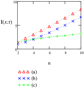
Figure 2: Information $I(x_{{\mathcal{M}}(G)}:F)$ for (a) $|G|=\sqrt{n}$,(b) $|G|=n$ and (c) $|G|=2^{n-\sqrt{n}}$

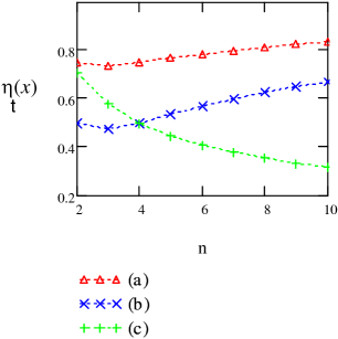
Figure 3: Efficiency $\eta_{F}(x_{{\mathcal{M}}(G)})$ for (a) $|G|=\sqrt{n}$,(b) $|G|=n$ and (c) $|G|=2^{n-\sqrt{n}}$

Let us first compare the information value and the efficiency of three subcases of this identity property with the following three different class cardinalities: $|G|=\sqrt{n}$, $|G|=n$ and $|G|=2^{n-\sqrt{n}}$. Figure 2 displays the information value and Figure 3 shows the efficiency for these subcases. As seen the information value increases as the cardinality of $G$ decreases which follows from (16). The efficiency $\eta_{F}(x)$ for these three subcases may be obtained exactly and equals (according to the same order as above) $1-(\log n)/(2n)$, $1-(\log n)/n$ and $1/\sqrt{n}$. Thus a property with a single element $G$ may have an efficiency which increases or decreases depending on the rate of growth of the cardinality of $G$ with respect to $n$.

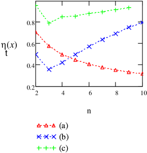
Figure 4: Efficiency $\eta_{F}(x)$ for (a) $x_{{\mathcal{L}}_{d}}$, (b) $x_{{{\mathcal{V}}}^{c}_{d}}$ and (c) $x_{{{\mathcal{V}}}_{d}}$, $d=\sqrt{n}$

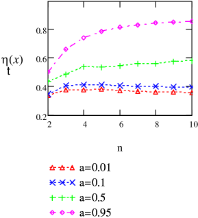
Figure 5: Efficiency $\eta_{F}(x_{{{\mathcal{V}}}_{d}(S_{m})})$, with $m=n^{a}$, $a=0.01,0.1,0.5,0.95$, $d=\sqrt{n}$

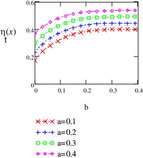
Figure 6: Efficiency $\eta_{F}(x_{{{\mathcal{V}}}_{d}(S_{m})})$, with $n=10$, $m(n)=m^{a}$, $d(n)=n^{b}$

Let us compare the efficiency for inputs $x_{{\mathcal{L}}_{d}}$, $x_{{{\mathcal{V}}}^{c}_{d}}$, $x_{{{\mathcal{V}}}_{d}}$ and $x_{{{\mathcal{V}}}_{d}(S_{m})}$. As an example, suppose that the VC-dimension parameter $d$ grows as $d(n)=\sqrt{n}$. As can be seen from Figure 4, property ${{\mathcal{V}}}_{d}$ is the most efficient of the three staying above the $80\%$ level. Letting the sample size increase at the rate of $m(n)=n^{a}$ then from Figure 5 the efficiency of ${\mathcal{V}}_{d}(S_{m})$ increases with respect to $a$ but remains smaller than the efficiency of property ${\mathcal{V}}_{d}$. Letting the VC-dimension increase as $d(n)=n^{b}$ then Figure 6 displays the efficiency of ${\mathcal{V}}_{d}(S_{m})$ as a function of $b$ for several values of $a=0.1,0.2,\ldots,0.4$ where $n$ is fixed at $10$. As seen, the efficiency increases approximately linearly with $a$ and non-linearly with respect to $b$ with a saturation at approximately $b=0.2$.

9 Conclusions

The information width introduced here is a fundamental concept based on which a combinatorial interpretation of information is defined and used as the basis for the concept of efficiency of information. We defined the width from two perspectives, that of the provider and the acquirer of information and used it as a reference point according to which the efficiency of any input information can be evaluated. As an application we considered the space of binary function classes on a finite domain and computed the efficiency of information conveyed by various class properties. The main point that arises from these results is that side-information of different types can be quantified, computed and compared in this common framework which is more general than the standard framework used in the theory of information transmission.

As further work, it will be interesting to compute the efficiency of information in other applications, for instance, pertaining to properties of classes of Boolean functions $f:\{0,1\}^{n}\rightarrow\{0,1\}$ (for which there are many applications, see for instance [8]). It will be interesting to examine standard search algorithms, for instance, those used in machine learning over a finite search space (or hypothesis space) and compute their information efficiency, i.e., accounting for all side information available for an algorithm (including data) and computing for it the acquired information value and efficiency.

In our treatment of this subject we did not touch the issue of how the information is used. For instance, a learning algorithm uses side-information and training data to learn a pattern classifier which has minimal prediction (generalization) error. A search algorithm in the area of information-retrieval uses an input query to return an answer set that overlaps as many of the relevant objects and at the same time has as few non-relevant objects as possible. In each such application the information acquirer, e.g., an algorithm, has an associated performance criterion, e.g., prediction error, percentage recall or precision, according to which it is evaluated. What is the relationship between information and performance, does performance depend on efficiency or only on the amount of provided information ? what are the consequences of using input information of low efficiency ? For the current work, we leave these questions as open. The remaining parts of the paper consist of the technical work used to obtain the previous results.

10 Technical results

In this section we provide the proofs of Theorems 2 to 5. Our approach is to estimate the number of sets $G\subseteq F$ that satisfy a property ${\mathcal{M}}$. Using the techniques from [28] we employ a probabilistic method by which a random class is generated and the probability that it satisfies ${\mathcal{M}}$ is computed. As we use the uniform probability distribution on elements of the power set ${\mathcal{P}}(F)$ then probabilities yield cardinalities of the corresponding sets. The computation of $\omega_{x}(k)$ and hence of (6) follows directly. It is worth noting that, as in [12], the notion of probability is only used here for simplifying some of the counting arguments and thus, unlike Shannon’s information, it plays no role in the actual definition of information.

Before proceeding with the proofs, in the next section we describe the probability model for generating a random class.

10.1 Random class generation

In this subsection we describe the underlying probabilistic processes with which a random class is generated. We use the so-called binomial model to generate a random class of binary functions (this has been extensively used in the area of random graphs [11]). In this model, the random class ${\mathcal{F}}$ is constructed through $2^{n}$ independent coin tossings, one for each function in $F$, with a probability of success (i.e., selecting a function into ${\mathcal{F}}$) equal to $p$. The probability distribution $P_{n,p}$ is formally defined on ${\mathcal{P}}(F)$ as follows: given parameters $n$ and $0\leq p\leq 1$, for any $G\in{\cal P}(F)$,

$$P_{n,p}({\mathcal{F}}=G)=p^{|G|}(1-p)^{2^{n}-|G|}.$$

In our application, we choose $p=1/2$ and denote the probability distribution as

$$P_{n}\equiv P_{n,\frac{1}{2}}.$$

It is clear that for any element $G\in{\mathcal{P}}(F)$, the probability that the random class ${\mathcal{F}}$ equals $G$ is

$$\alpha_{n}\equiv P_{n}({\mathcal{F}}=G)=\left(\frac{1}{2}\right)^{2^{n}}$$ (17)

and the probability of ${\mathcal{F}}$ having a cardinality $k$ is

$$P_{n}(|{\mathcal{F}}|=k)={2^{n}\choose k}\alpha_{n},\;\;1\leq k\leq 2^{n}.$$ (18)

The following fact easily follows from the definition of the conditional probability: for any set $B\subseteq{\cal P}(F)$,

$$P_{n}({\mathcal{F}}\in B|\;|{\mathcal{F}}|=k)=\frac{\sum_{G\in B}\alpha_{n}}{{2^{n}\choose k}\alpha_{n}}=\frac{|B|}{{2^{n}\choose k}}.$$ (19)

Denote by

$$F^{(k)}=\{G\in{\mathcal{P}}(F):|G|=k\},$$

the collection of binary-function classes of cardinality $k$, $1\leq k\leq 2^{n}$. Consider the uniform probability distribution on $F^{(k)}$ which is defined as follows: given parameters $n$ and $1\leq k\leq 2^{n}$ then for any $G\in{\cal P}(F)$,

$$P^{*}_{n,k}(G)=\frac{1}{\binom{2^{n}}{k}},\mbox{ if }G\in{F}^{(k)},$$ (20)

and $P^{*}_{n,k}(G)=0$ otherwise. Hence from (19) and (20) it follows that for any $B\subseteq{\mathcal{P}}(F)$,

$$P_{n}({\mathcal{F}}\in B|\;|{\mathcal{F}}|=k)=P^{*}_{n,k}({\mathcal{F}}\in B).$$ (21)

It will be convenient to use another probability distribution which estimates $P^{*}_{n,k}$ and is defined as follows. Construct a random $n\times k$ binary matrix by fair-coin tossings with the $nk$ elements taking values $0$ or $1$ independently with probability $1/2$. Denoting by $Q^{*}_{n,k}$ the probability measure corresponding to this process then for any matrix $U\in{\cal U}_{n\times k}(\{0,1\})$,

$$Q^{*}_{n,k}(U)=\frac{1}{2^{nk}}.$$

Clearly, the columns of a binary matrix $U$ are vectors of length $n$ which are binary functions on $[n]$. Hence the set $\text{cols}(U)$ of columns of $U$ represents a class of binary functions. It contains $k$ elements if and only if $\text{cols}(U)$ consists of distinct elements, or less than $k$ elements if two columns are the same. Denote by $S$ a simple binary matrix as one all of whose columns are distinct ([1]). We claim that the conditional distribution of the set of columns of a random binary matrix, knowing that the matrix is simple, is the uniform probability distribution $P^{*}_{n,k}$. To see this, observe that the probability that the columns of a random binary matrix are distinct is

$$Q^{*}_{n,k}(S)=\frac{2^{n}(2^{n}-1)\cdots(2^{n}-k+1)}{2^{nk}}.$$ (22)

For any fixed class $G\in{\mathcal{P}}(F)$ of $k$ binary functions there are $k!$ corresponding simple matrices in ${\cal U}_{n\times k}(\{0,1\})$. Therefore given a simple matrix $S$, the probability that $\text{cols}(S)$ equals a class $G$ is

$$Q^{*}_{n,k}(G|S)=\frac{k!}{2^{nk}}\frac{2^{nk}}{2^{n}(2^{n}-1)\cdots(2^{n}-k+1)}=\frac{1}{\binom{2^{n}}{k}}=P^{*}_{n,k}(G).$$ (23)

Using the distribution $Q^{*}_{n,k}$ enables simpler computations of the asymptotic probability of several types of events that are associated with the properties of Theorems 2 – 5. We henceforth resort to the following process for generating a random class $G$: for every $1\leq k\leq 2^{n}$ we repeatedly and independently draw matrices of size $n\times k$ using $Q^{*}_{n,k}$ until we get a simple matrix $M_{n\times k}$. Then we randomly draw a value for $k$ according to the distribution of (18) and choose the formerly generated simple matrix corresponding to this chosen $k$. Since this is a simple matrix then by (23) it is clear that this choice yields a random class $G$ which is distributed uniformly in $F^{(k)}$ according to $P^{*}_{n,k}$. This is stated formally in Lemma 3 below but first we have an auxiliary lemma that shows the above process converges.

Lemma 2

Let $n=1,2,\ldots$ and consider the process of drawing sequences $s^{(k)}_{m}=\{M^{(i)}_{k,n}\}_{i=1}^{m}$, $1\leq k\leq 2^{n}$, all of length $m$ where the $k^{th}$ sequence consists of matrices $M^{(i)}_{k,n}\in\mathcal{U}_{n\times k}(\{0,1\})$ which are randomly and independently drawn according to the probability distribution $Q^{*}_{n,k}$. Then the probability that after $m=ne^{2^{n}}$ trials there exists a $k$ such that no simple matrix appears in $s^{(k)}_{m}$, converges to zero with increasing $n$.

Proof: Let $a({n,k})=Q^{*}_{n,k}(S)$ be the probability of getting a simple matrix $M_{n,k}\in\mathcal{U}_{n\times k}$. Then the probability that there exists some $k$ such that $s^{(k)}_{m}$ consists of only non-simple matrices is

$$q(n,m)\leq\sum_{k=1}^{2^{n}}(1-a({n,k}))^{m}\leq\sum_{k=1}^{2^{n}}e^{-ma(n,k)}.$$ (24)

From (22) we have

$$\ln a(n,k)=\sum_{i=0}^{k-1}\ln(2^{n}-i)-nk\ln 2=\sum_{j=2^{n}-(k-1)}^{2^{n}}\ln j-nk\ln 2.$$ (25)

Since $\ln x$ is increasing function of $x$ then for any pair of positive integers $2\leq a\leq b$ we have

$$\sum_{j=a}^{b}\ln j\geq\int_{a-1}^{b}\ln xdx=b(\ln b-1)-(a-1)(\ln(a-1)-1).$$

Hence

$$\ln a(n,k)\geq 2^{n}(n\ln 2-1)-(2^{n}-k)(\ln(2^{n}-k)-1)-nk\ln 2\equiv b(n,k)$$

and the right side of (24) is now bounded as follows

$$\sum_{k=1}^{2^{n}}e^{-ma(n,k)}\leq\sum_{k=1}^{2^{n}}e^{-me^{b(n,k)}}.$$ (26)

From a simple check of the derivative of $b(n,k)$ with respect to $k$ it follows that $b(n,k)$ is a decreasing function of $k$ on $1\leq k\leq 2^{n}$. Replacing each term in the sum on the right side of (26) by the last term gives the following bound

$$q(n,m)\leq e^{n\ln 2-me^{-2^{n}}}.$$ (27)

The exponent is negative provided

$$m>n\ln(2)e^{2^{n}}.$$

Choosing $m=ne^{2^{n}}$ guarantees that $q(n,m)\rightarrow 0$ with increasing $n$. $\square$

The following result states that the measure $Q^{*}_{n,k}$ may replace $P^{*}_{n,k}$ uniformly over $1\leq k\leq 2^{n}$.

Lemma 3

Let $B\subseteq{\cal P}(F)$. Then

$$\max_{1\leq k\leq 2^{n}}|P^{*}_{n,k}(B)-Q^{*}_{n,k}(B)|\rightarrow 0$$

as $n$ tends to infinity.

Proof: From (23) we have

$$P^{*}_{n,k}(B)=Q^{*}_{n,k}(B|S)=\frac{Q^{*}_{n,k}(B\bigcap S)}{Q^{*}_{n,k}(S)}.$$

Then

$$\max_{k}|P^{*}_{n,k}(B)-Q^{*}_{n,k}(B)|=\max_{k}\left|\frac{Q^{*}_{n,k}(B\bigcap S)}{Q^{*}_{n,k}(S)}-Q^{*}_{n,k}(B)\right|$$ (28)

$$\leq \max_{k}\left|\frac{1}{Q^{*}_{n,k}(S)}\right|\max_{k}\left|Q^{*}_{n,k}(B\bigcap S)-Q^{*}_{n,k}(B)Q^{*}_{n,k}(S)\right|$$

$$\leq \max_{k}\left|\frac{1}{Q^{*}_{n,k}(S)}\right|\Biggl{(}\max_{k}\left|Q^{*}_{n,k}(B\bigcap S)-Q^{*}_{n,k}(B)\right|+\max_{k}\left|Q^{*}_{n,k}(B)(1-Q^{*}_{n,k}(S))\right|\Biggr{)}$$

$$\leq \max_{k}\left|\frac{1}{Q^{*}_{n,k}(S)}\right|\Biggl{(}\max_{k}\left|Q^{*}_{n,k}(B\bigcap S)-Q^{*}_{n,k}(B)\right|+\max_{k}\left|Q^{*}_{n,k}(B)\right|\max_{k}\left|1-Q^{*}_{n,k}(S)\right|\Biggr{)}.\quad\quad$$

From Lemma 2 it follows that

$$\max_{k}\left|1-Q^{*}_{n,k}(S)\right|\rightarrow 0,\qquad\max_{k}|1/Q^{*}_{n,k}(S)|\rightarrow 1$$ (29)

with increasing $n$. For any $1\leq k\leq 2^{n}$,

$$Q^{*}_{n,k}(B)+Q^{*}_{n,k}(S)-1\leq Q^{*}_{n,k}(B\bigcap S)\leq Q^{*}_{n,k}(B)$$

and by Lemma 2, $Q^{*}_{n,k}(S)$ tends to $1$ uniformly over $1\leq k\leq 2^{n}$ with increasing $n$. Hence $\max_{k}\left|Q^{*}_{n,k}(B\bigcap S)-Q^{*}_{n,k}(B)\right|\rightarrow 0$ which together with (28) and (29) implies the statement of the lemma. $\square$ We now proceed to the proofs of the theorems in Section 7.

10.2 Proofs

Note that for any property ${\mathcal{M}}$, the quantity $\omega_{x}(k)$ in (6) is the ratio of the number of classes $G\in F^{(k)}$ that satisfy ${\mathcal{M}}$ to the total number of classes that satisfy ${\mathcal{M}}$. It is therefore equal to $P_{n}(|{\mathcal{F}}|=k\,|\,{\mathcal{F}}\models{\mathcal{M}})$. Our approach starts by computing the probability $P_{n}({\mathcal{F}}\models{\mathcal{M}}\,|\,|{\mathcal{F}}|=k)$ from which $P_{n}(|{\mathcal{F}}|=k\,|\,{\mathcal{F}}\models{\mathcal{M}})$ and then $\omega_{x}(k)$ are obtained.

10.2.1 Proof of Theorem 2

We start with an auxiliary lemma which states that the probability $P_{n}({\mathcal{F}}\models{\mathcal{L}}_{d}\,|\,|{\mathcal{F}}|=k)$ possesses a zero-one behavior.

Lemma 4

Let ${\mathcal{F}}$ be a class of cardinality $k_{n}$ and randomly drawn according to the uniform probability distribution $P^{*}_{n,k_{n}}$ on $F^{(k_{n})}$. Then as $n$ increases, the probability $P^{*}_{n,k_{n}}({\mathcal{F}}\models{\mathcal{L}}_{d})$ that ${\mathcal{F}}$ satisfies property ${\mathcal{L}}_{d}$ tends to $0$ or $1$ if $k_{n}\gg\log(2n/d)$ or $k_{n}=1+\kappa_{n}$, $\kappa_{n}\ll(\log(n))/d$, respectively.

Proof: For brevity, we sometimes write $k$ for $k_{n}$. Using Lemma 3 it suffices to show that $Q^{*}_{n,k}({\mathcal{F}}\models{\mathcal{L}}_{d})$ tends to $1$ or $0$ under the stated conditions. For any set $S\subseteq[n]$, $|S|=d$ and any fixed $v\in\{0,1\}^{d}$, under the probability distribution $Q^{*}_{n,k}$, the event $E_{v}$ that every function $f\in{\mathcal{F}}$ satisfies $f_{|S}=v$ has a probability $(1/2)^{kd}$. Denote by $E_{S}$ the event that all functions in the random class ${\mathcal{F}}$ have the same restriction on $S$. There are $2^{d}$ possible restrictions on $S$ and the events $E_{v}$, $v\in\{0,1\}^{d}$, are disjoint. Hence $Q^{*}_{n,k}(E_{S})=2^{d}(1/2)^{kd}=2^{-(k-1)d}$. The event that ${\mathcal{F}}$ has property ${\mathcal{L}}_{d}$, i.e., that $L({\mathcal{F}})\geq d$, equals the union of $E_{S}$, over all $S\subseteq[n]$ of cardinality $d$. Thus we have

$$Q^{*}_{n,k}({\mathcal{F}}\models{\mathcal{L}}_{d}) = Q^{*}_{n,k}\left(\bigcup_{S\subseteq[n]:|S|=d}E_{S}\right)$$

$$\leq {n\choose d}Q^{*}_{n,k}\left(E_{[d]}\right)=2^{-(k-1)d}\frac{n^{d}(1-o(1))}{d!}.$$

For $k=k_{n}\gg\log(2n/d)$ the right side tends to zero which proves the first statement. Let the mutually disjoint sets $S_{i}=\{id+1,id+2,\ldots,d(i+1)\}\subseteq[n]$, $0\leq i\leq m-1$ where $m=\lfloor n/d\rfloor$. The event that ${\mathcal{M}}_{d}$ is not true equals $\bigcap_{S:|S|=d}\overline{E}_{S}$. Its probability is

$$Q^{*}_{n,k}\left(\bigcap_{S:|S|=d}\overline{E}_{S}\right) = 1-Q^{*}_{n,k}\left(\bigcup_{S:|S|=d}{E}_{S}\right)\leq\max\{0,1-Q^{*}_{n,k}\left(\bigcup_{i=0}^{m-1}{E}_{S_{i}}\right)\}.$$

Since the sets are disjoint and of the same size $d$ then the right hand side equals $\max\{0,1-mQ^{*}_{n,k}({E}_{[d]})\}$. This equals

$$\max\{0,1-\left\lfloor\frac{n}{d}\right\rfloor 2^{-(k-1)d}\}$$

which tends to zero when $k=k_{n}=1+\kappa_{n}$, $\kappa_{n}\ll(\log(n))/d$. The second statement is proved. $\square$

Remark 12

While from this result it is clear that the critical value of $k$ for the conditional probability $P_{n}({\mathcal{L}}_{d}|k)$ to tend to $1$ is $O(\log(n))$, as will be shown below, when considering the conditional probability $P_{n}(k|{\mathcal{L}}_{d})$, the most probable value of $k$ is much higher at $O(2^{n-d})$.

We continue now with the proof of Theorem 2. For any probability measure $\mathbb{P}$ on ${\mathcal{P}}(F)$ denote by $\mathbb{P}(k|{\mathcal{L}}_{d})=\mathbb{P}(|{\mathcal{F}}|=k\,|\,{\mathcal{F}}\models{\mathcal{L}}_{d}).$ By the premise of Theorem 2, the input $x$ describes the target $t$ as an element of a class that satisfies property ${\mathcal{L}}_{d}$. In this case the quantity $\omega_{x}(k)$ is the ratio of the number of classes of cardinality $k$ that satisfy ${\mathcal{L}}_{d}$ to the total number of classes that satisfy ${\mathcal{L}}_{d}$. Since by (17) the probability distribution $P_{n}$ is uniform over the space ${\mathcal{P}}(F)$ whose size is $2^{2^{n}}$ then

$$\omega_{x}(k)=\frac{P_{n}(k,{\mathcal{L}}_{d})2^{2^{n}}}{P_{n}({\mathcal{L}}_{d})2^{2^{n}}}=P_{n}(k|{\mathcal{L}}_{d}).$$ (30)

We have

$$P_{n}(k|{\mathcal{L}}_{d})=\frac{P_{n}({\mathcal{L}}_{d}|k)P_{n}(k)}{\sum_{j=1}^{2^{n}}P_{n}({\mathcal{L}}_{d}|j)P_{n}(j)}.$$

By (21), it follows therefore that the sum in (6) equals

$$\sum_{k=2}^{2^{n}}\omega_{x}(k)\log(k)=\sum_{k=2}^{2^{n}}\frac{P^{*}_{n,k}({\mathcal{L}}_{d})P_{n}(k)}{\sum_{j=1}^{2^{n}}P^{*}_{n,j}({\mathcal{L}}_{d})P_{n}(j)}\log k.$$ (31)

Let $N=2^{n}$, then by Lemma 3 and from the proof of Lemma 4, as $n$ (hence $N$) increases, it follows that

$$P^{*}_{n,k}({\mathcal{L}}_{d})\approx Q^{*}_{n,k}({\mathcal{L}}_{d})=\left(\frac{1}{2}\right)^{d(k-1)}A(N,d)$$ (32)

where $A(N,d)$ satisfies

$$\frac{\log N}{d}\leq A(N,d)\leq\frac{\log^{d}N}{d!}.$$

Let $p=1/(1+2^{d})$ then using (32) the ratio in (31) is

$$\frac{\sum_{k=2}^{N}{N\choose k}p^{k}(1-p)^{N-k}\log k}{\sum_{j=1}^{N}{N\choose j}p^{j}(1-p)^{N-j}}.$$ (33)

Substituting for $N$ and $p$, the denominator equals

$$1-(1-p)^{N}=1-\left(1-\frac{1}{1+2^{d}}\right)^{2^{n}}=1-\left(\frac{2^{d}}{1+2^{d}}\right)^{2^{n}}.$$ (34)

Using the DeMoivre-Laplace limit theorem [9], the binomial distribution $P_{N,p}(k)$ with parameters $N$ and $p$ satisfies

$$P_{N,p}(k)\approx\frac{1}{\sigma}\phi\left(\frac{k-\mu}{\sigma}\right),\;\;N\rightarrow\infty$$

where $\phi(x)=(1/\sqrt{2\pi})\exp(-x^{2}/2)$ is the standard normal probability density function and $\mu=Np$, $\sigma=\sqrt{Np(1-p)}$. The sum in the numerator of (33) may be approximated by an integral

$$\frac{1}{\sigma}\int_{2}^{\infty}\phi\left(\frac{x-\mu}{\sigma}\right)\log x\,dx=\int_{(2-\mu)/\sigma}^{\infty}\phi(x)\log(\sigma x+\mu)dx.$$

The $\log$ factor equals $\log\mu$ + $\log(1+x\sigma/\mu)=\log\mu+x\sigma/\mu+O(x^{2}(\sigma/\mu)^{2})$. Denote by $a=(2-\mu)/\sigma$ then the right side above equals

$$\Phi(-a)\log\mu+\frac{\sigma}{\mu}\phi(a)+O\left(\left(\frac{\sigma}{\mu}\right)^{2}\right)$$

where $\Phi(x)$ is the normal cumulative probability distribution. Substituting for $\mu$, $\sigma$, $p$ and $N$, and combining with (34) then (31) is asymptotically equal to

$$\sum_{k=2}^{2^{n}}\omega_{x}(k)\log k\approx\frac{\Phi\left(-a\right)\log\left(\frac{2^{n}}{1+2^{d}}\right)+2^{-(n-d)/2}\phi(a)+O(2^{-(n-d)})}{1-\left(\frac{2^{d}}{1+2^{d}}\right)^{2^{n}}}$$ (35)

where

$$a=2(1+2^{d})2^{-(n+d)/2}-2^{(n-d)/2}.$$

In Theorem 2, the set $\mathbb{Y}$ is the class $F$ (see (6)) hence $\log|F|=n$ and

$$I(x:F) = n-\sum_{k\geq 2}\omega_{x}(k)\log k.$$

Combining with (35) the first statement of Theorem 2 follows.

We now compute the description complexity $\ell(x_{{\mathcal{L}}_{d}})$. Since in this setting $\mathbb{Y}$ is $F$ and $\mathbb{Z}$ is ${\mathcal{P}}(F)$ then, by (9), the description complexity $\ell(x_{{\mathcal{L}}_{d}})$ is $2^{n}-\log|{\mathcal{L}}_{d}|$. Since , the probability distribution $P_{n}$ is uniform on ${\mathcal{P}}(F)$ then the cardinality of ${\mathcal{L}}_{d}$ equals

$$|{\mathcal{L}}_{d}|=2^{2^{n}}P_{n}({\mathcal{L}}_{d}).$$

It follows that

$$\ell(x_{{\mathcal{L}}_{d}})=-\log P_{n}({\mathcal{L}}_{d})$$

hence it suffices to compute $P_{n}({\mathcal{L}}_{d})$. Letting $N=2^{n}$, we have

$$P_{n}({\mathcal{L}}_{d})=\sum_{k=1}^{N}P_{n}({\mathcal{L}}_{d}|k)P_{N}(k)=\sum_{k=1}^{N}P^{*}_{n,k}({\mathcal{L}}_{d})P_{N}(k).$$

Using (32) and letting $p=1/(1+2^{d})$ this becomes

$$\sum_{k=1}^{N}\left(\frac{1}{2}\right)^{d(k-1)}A(N,d)\left(\frac{1}{2}\right)^{N}{N\choose k}$$

$$= \left(\frac{1}{1-p}\right)^{N}\left(\frac{1}{2}\right)^{N-d}A(N,d)(1-(1-p)^{N}).$$

Letting $q=(1-p)^{N}$, it follows that

$$-\log P_{n}({\mathcal{L}}_{d}) = \log\left(\frac{2^{N-d}}{A(N,d)}\right)+\log\left(\frac{q}{1-q}\right)$$

$$= N-d-\log A(N,d)+q+O(q^{2})+\log(q)$$

$$= N(1-p-O(p^{2}))-d-c\log\log N+o(1)$$

where $1\leq c\leq d$. Substituting for $N$ gives the result.     $\blacksquare$

10.2.2 Proof of Theorem 3

We start with an auxiliary lemma that states a threshold value for the cardinality of a random element of $F^{(k)}$ that satisfies property ${{\mathcal{V}}}^{c}_{d}$.

Lemma 5

For any integer $d>0$ let $k$ be an integer satisfying $k\geq 2^{d}$. Let ${\mathcal{F}}$ be a class of cardinality $k$ and randomly drawn according to the uniform probability distribution $P^{*}_{n,k}$ on $F^{(k)}$. Then

$$\lim_{n\rightarrow\infty}P^{*}_{n,k}({{\mathcal{V}}}^{c}_{d})=1.$$

Remark 13

When $k_{n}<2^{d}$ there does not exist an $E\subseteq[n]$ with $|\text{tr}_{E}({\mathcal{F}})|=2^{d}$ hence $P^{*}_{n,k_{n}}({{\mathcal{V}}}^{c}_{d})=0$. For $k_{n}\gg 2^{d}$, $P^{*}_{n,k_{n}}({{\mathcal{V}}}^{c}_{d})$ tends to $1$. Hence, for a random class ${\mathcal{F}}$ to have property ${{\mathcal{V}}}^{c}_{d}$ the critical value of its cardinality is $2^{d}$.

We proceed now with the proof of Lemma 5. Proof: It suffices to prove the result for $k=2^{d}$ since $P^{*}_{n,k}({\mathcal{F}}\models{{\mathcal{V}}}^{c}_{d})\geq P^{*}_{n,2^{d}}({\mathcal{F}}\models{{\mathcal{V}}}^{c}_{d})$. As in the proof of Lemma 4, we represent $P^{*}_{n,2^{d}}$ by $Q^{*}_{n,2^{d}}$ using (23) and with Lemma 3 it suffices to show that $Q^{*}_{n,2^{d}}({\mathcal{F}}\models{{\mathcal{V}}}^{c}_{d})$ tends to $1$. Denote by $U_{d}$ the ‘complete’ matrix with $d$ rows and $2^{d}$ columns formed by all $2^{d}$ binary vectors of length $d$, ranked for instance in alphabetical order. The event “${\mathcal{F}}\models{{\mathcal{V}}}^{c}_{d}$” occurs if there exists a subset $S=\{i_{1},\ldots,i_{d}\}\subseteq[n]$ such that the submatrix whose rows are indexed by $S$ and columns by $[2^{d}]$, is equal to $U_{d}$. Let $S_{i}=\{id+1,id+2,\ldots,d(i+1)\}$, $0\leq i\leq m-1$, be the sets defined in the proof of Lemma 4 and consider the $m$ corresponding events which are defined as follows: the $i^{th}$ event is described as having a submatrix whose rows are indexed by $S_{i}$ and is equal to $U_{d}$. Since the sets $S_{i}$, $1\leq i\leq m$ are disjoint it is clear that these events are independent and have the same probability

$$Q^{*}_{n,k}(S_{i})=2^{-d2^{d}}.$$

Hence the probability that at least one of them is fulfilled is

$$1-(1-2^{-d2^{d}})^{\lfloor n/d\rfloor}$$

which tends to $1$ as $n$ increases. $\square$ We continue with the proof of Theorem 3. As in the proof of Theorem 2, since by (17) the probability distribution $P_{n}$ is uniform over ${\mathcal{P}}(F)$ then

$$\omega_{x}(k)=\frac{P_{n}(k,{{\mathcal{V}}}^{c}_{d})2^{2^{n}}}{P_{n}({{\mathcal{V}}}^{c}_{d})2^{2^{n}}}=P_{n}(k|{{\mathcal{V}}}^{c}_{d})=\frac{P^{*}_{n,k}({{\mathcal{V}}}^{c}_{d})P_{n}(k)}{\sum_{j=0}^{2^{n}}P^{*}_{n,j}({{\mathcal{V}}}^{c}_{d})P_{n}(j)},1\leq k\leq 2^{n}.$$

Considering Remark 13, in this case the sum in (6) is

$$\sum_{k=2^{d}}^{2^{n}}\frac{P^{*}_{n,k}({{\mathcal{V}}}^{c}_{d})P_{n}(k)\log k}{\sum_{j=2^{d}}^{2^{n}}P^{*}_{n,j}({{\mathcal{V}}}^{c}_{d})P_{n}(j)}.$$ (36)

We now obtain its asymptotic value as $n$ increases. From the proof of Lemma 5, it follows that for all $k\geq 2^{d}$,

$$P^{*}_{n,k}({{\mathcal{V}}}^{c}_{d})\approx 1-(1-\beta)^{rk},\;\beta=2^{-d2^{d}},r={\frac{n}{d2^{d}}}.$$

Since $\beta$ is an exponentially small positive real we approximate $(1-\beta)^{rk}$ by $1-rk\beta$ (by assumption, $n<d2^{d}$ hence this remains positive for all $1\leq k\leq 2^{n}$). Therefore we take

$$P^{*}_{n,k}({{\mathcal{V}}}^{c}_{d})\approx rk\beta$$ (37)

and (36) is approximated by

$$\frac{\sum_{k=2^{d}}^{2^{n}}kP_{n}(k)\log k}{\sum_{j=2^{d}}^{2^{n}}jP_{n}(j)}.$$ (38)

As before, for simpler notation let us denote $N=2^{n}$ and let $P_{N}(k)$ be the binomial distribution with parameters $N$ and $p=1/2$. Denote by $\mu=N/2$ and $\sigma=\sqrt{N/4}$, then using the DeMoivre-Laplace limit theorem we have

$$P_{N}(k)\approx\frac{1}{\sigma}\phi\left(\frac{k-\mu}{\sigma}\right),\;N\rightarrow\infty.$$

Thus (38) is approximated by the ratio of two integrals

$$\frac{\int_{(2^{d}-\mu)/\sigma}^{\infty}\phi(x)(\sigma x+\mu)\log(\sigma x+\mu)dx}{\int_{(2^{d}-\mu)/\sigma}^{\infty}\phi(x)(\sigma x+\mu)dx}.$$ (39)

The $\log$ factor equals $\log\mu$ + $\log(1+x\sigma/\mu)=\log\mu+x\sigma/\mu+O(x^{2}(\sigma/\mu)^{2})$. Denote by

$$a=(\mu-2^{d})/\sigma$$ (40)

then the numerator is approximated by

$$\Phi(a)\mu\log\mu+\sigma(1+\log\mu)\phi(a)+O\left(\frac{\sigma^{3}}{\mu^{2}}a^{2}\phi(a)\right)$$

$$= \log(N/2)\left(\Phi(a)N/2+\left(1+\frac{a^{2}}{N\log(N/2)}\right)\phi(a)\sqrt{N}/2\right).$$

Similarly, the denominator of (39) is approximated by $\Phi(a)N/2+\phi(a)\sqrt{N}/2.$ The ratio, and hence (36), tends to

$$\frac{\log(N/2)\left(\Phi(a)N/2+\left(1+\frac{a^{2}}{N\log(N/2)}\right)\phi(a)\sqrt{N}/2\right)}{\Phi(a)N/2+\phi(a)\sqrt{N}/2}.$$

Substituting back for $a$ then the above tends to $\log(N/2)=\log N-1$. With $N=2^{n}$ and (6) the first statement of the theorem follows.

We now compute the description complexity $\ell(x_{{{\mathcal{V}}}^{c}_{d}})$. Following the steps of the second part of the proof of Theorem 2 (Section 10.2.1) we have $\ell(x_{{{\mathcal{V}}}^{c}_{d}})=-\log P_{n}({{\mathcal{V}}}^{c}_{d})$. Using (37) the probability is approximated by

$$P_{n}({{\mathcal{V}}}^{c}_{d})\approx r\beta\sum_{k=2^{d}}^{N}kP_{N}(k)$$

and as before, this is approximated by $r\beta(\Phi(a)N+\phi(a)\sqrt{N})/2$. Thus substituting for $r$ and $\beta$ we have

$$-\log P_{n}({{\mathcal{V}}}^{c}_{d})\approx d(2^{d}+1)+\log(d)-\log\left(\Phi(a)N+\phi(a)\sqrt{N}\right)-\log\log N+1.$$

Substituting for $N$ yields the result.     $\blacksquare$

10.2.3 Proof of Theorem 4

The proof is almost identical to that of Theorem 3. From (37) we have

$$P^{*}_{n,k}({{\mathcal{V}}}_{d})=1-P^{*}_{n,k}({{\mathcal{V}}}^{c}_{d})=\left\{\begin{array}[]{ll}1&,1\leq k<2^{d}\\ 1-P^{*}_{n,k}({\mathcal{V}}_{d}^{c})\approx 1-r\beta k&,2^{d}\leq k\leq 2^{n}\end{array}\right.$$

hence

$$\sum_{k=2}^{2^{n}}\frac{P^{*}_{n,k}({{\mathcal{V}}}_{d})P_{n}(k)\log k}{\sum_{j=1}^{2^{n}}P^{*}_{n,j}({{\mathcal{V}}}_{d})P_{n}(j)}\approx\frac{\sum_{k=2}^{2^{n}}P_{n}(k)\log k-r\beta\sum_{k=2^{d}}^{2^{n}}kP_{n}(k)\log k}{\sum_{j=1}^{2^{n}}P_{n}(j)-r\beta\sum_{j=2^{d}}^{2^{n}}jP_{n}(j)}.$$ (41)

Let $a$ be as in (40) and denote by $b=(\mu-2)/\sigma$ and

$$s=\Phi(a)N/2+\phi(a)\sqrt{N}/2$$

then the numerator tends to $\log(N/2)(\Phi(b)-rs\beta)+\phi(b)/\sqrt{N}$ and the denominator tends to $1-(1/2)^{N}-rs\beta$. Then (41) tends to

$$\log(N/2)\frac{\Phi(b)-rs\beta}{1-rs\beta}+\frac{\phi(b)}{\sqrt{N}\left(1-(1/2)^{N}-rs\beta\right)}\approx\log(N/2)+\frac{\phi(b)}{\sqrt{N}(1-rs\beta)}.$$

Substituting for $r$, $\beta$ and $N$ yields the statement of the theorem.     $\blacksquare$

10.2.4 Proof of Theorem 5

The probability that a random class of cardinality $k$ satisfies the property ${\mathcal{V}}_{d}(S_{m})$ is

$$P_{n}({\mathcal{F}}\models{\mathcal{V}}_{d}(S_{m})\;|\;|{\mathcal{F}}|=k)=P_{n}({\mathcal{F}}\models{\mathcal{V}}_{d},{\mathcal{F}}_{|\xi}=\zeta\;|\;|{\mathcal{F}}|=k)$$ (42)

$$= P_{n}({\mathcal{F}}\models{\mathcal{V}}_{d}\;|\;{\mathcal{F}}_{|\xi}=\zeta,|{\mathcal{F}}|=k)P_{n}({\mathcal{F}}_{|\xi}=\zeta\;|\;|{\mathcal{F}}|=k).$$

The factor on the right of (42) is the probability of the condition $E_{\zeta}$ that a random class ${\mathcal{F}}$ of size $k$ has for all its elements the same restriction $\zeta$ on the sample $\xi$. As in the proof of Lemma 4 it suffices to use the probability distribution $Q^{*}_{n,k}$ in which case $Q^{*}_{n,k}(E_{\zeta})$ is $\gamma^{k}$ where $\gamma\equiv(1/2)^{m}$. The left factor of (42) is the probability that a random class ${\mathcal{F}}$ with cardinality $k$ which satisfies $E_{\zeta}$ will satisfy property ${\mathcal{V}}_{d}$. This is the same as the event that a random class ${\mathcal{F}}$ on $[n]\setminus S_{m}$ satisfies property ${\mathcal{V}}_{d}$. Its probability is $P^{*}_{n-m,k}({\mathcal{V}}_{d})$ which equals $1$ for $k<2^{d}$ and using (37) for $k\geq 2^{d}$ it is approximated as

$$1-P^{*}_{n-m,k}({{\mathcal{V}}}^{c}_{d})\approx 1-rk\beta$$

where $r=(n-m)/(d2^{d})$ and $\beta=2^{-d2^{d}}$. Hence the conditional entropy becomes

$$\sum_{k=2}^{2^{n}}\frac{\gamma^{k}P^{*}_{n-m,k}({{\mathcal{V}}}_{d})P_{n}(k)\log k}{\sum_{j=1}^{2^{n}}\gamma^{j}P^{*}_{n-m,j}({{\mathcal{V}}}_{d})P_{n}(j)}\approx\frac{\sum_{k=2}^{2^{n}}\gamma^{k}P_{n}(k)\log k-r\beta\sum_{k=2^{d}}^{2^{n}}\gamma^{k}kP_{n}(k)\log k}{\sum_{j=1}^{2^{n}}\gamma^{j}P_{n}(j)-r\beta\sum_{j=2^{d}}^{2^{n}}\gamma^{j}jP_{n}(j)}.$$ (43)

Let $p=\gamma/(1+\gamma)$, $N=2^{n}$ and denote by $P_{N,p}(k)$ the binomial distribution with parameters $N$ and $p$. Then (43) becomes

$$\frac{\sum_{k=2}^{N}P_{N,p}(k)\log k-r\beta\sum_{k=2^{d}}^{N}kP_{N,p}(k)\log k}{\sum_{j=1}^{N}P_{N,p}(j)-r\beta\sum_{j=2^{d}}^{N}jP_{N,p}(j)}.$$ (44)

With $\mu=Np$ and $\sigma=\sqrt{Np(1-p)}$ let $a=(\mu-2^{d})/\sigma$, $b=(\mu-2)/\sigma$ and

$$s=\Phi(a)Np+\phi(a)\sqrt{Np(1-p)}$$

then the numerator tends to

$$\log(Np)(\Phi(b)-rs\beta)+\frac{\phi(b)}{\sqrt{N}}\sqrt{\frac{1-p}{p}}$$

and the denominator tends to $1-(2^{m}/(2^{m}+1))^{N}-rs\beta$. Therefore (44) tends to

$$\log(Np)+\frac{\phi(b)}{\sqrt{N}\left(1-o(1)-rs\beta\right)}\sqrt{\frac{1-p}{p}}.$$

Substituting for $r$, $s$, $\beta$ and $N$ yields the first statement of the theorem.

Next, we obtain the description complexity. We have

$$\ell(x_{{\mathcal{V}}_{d}(S_{m})})=-\log P_{n}({\mathcal{V}}_{d}(S_{m})).$$

The probability $P_{n}({\mathcal{V}}_{d}(S_{m}))$ is the denominator of (43) which equals the denominator of (44) multiplied by a factor of $(2(1-p))^{-N}$ hence from above

$$-\log P_{n}({\mathcal{V}}_{d}(S_{m}))\approx-\log\left(1-\left(\frac{2^{m}}{1+2^{m}}\right)^{N}-r\beta s\right)+N+N\log\left(1-p\right).$$

Let $q=\left(\frac{2^{m}}{1+2^{m}}\right)^{N}+r\beta s$ then we have as an estimate

$$\ell(x_{{\mathcal{V}}_{d}(S_{m})})\approx\log\left(\frac{1}{1-q}\right)+N(1+\log(1-p))$$

from which the second statement of the theorem follows.     $\blacksquare$

11 Acknowledgements

The author thanks Dr. Vitaly Maiorov from the department of mathematics of the Technion for useful remarks.

Figures

$\begin{array}[]{c@{\hspace{.1in}}c}\lx@intercol\hfil\lx@intercol&\lx@intercol\hfil\lx@intercol\\ \includegraphics[clip={true},scale={1},angle={90}]{fig1a.pdf}\hfil\hskip 7.22743pt&{\includegraphics[clip={true},scale={1},angle={90}]{fig1b.pdf}}\end{array}$

Figure 1: (a) $I^{*}(\ell)$,    (b) $\kappa^{*}(\ell)$

References

- [1] R. Anstee, B. Fleming, Z. Furedi, and A. Sali. Color critical hypergraphs and forbidden configurations. In Proc. EuroComb’2005, pages 117– 122. DMTCS, 2005.
- [2] M. Anthony and P. L. Bartlett. Neural Network Learning:Theoretical Foundations. Cambridge University Press, 1999.
- [3] M. Anthony, G. Brightwell, and C. Cooper. The Vapnik-Chervonenkis dimension of a random graph. Discrete Mathematics, 138(1-3):43–56, 1995.
- [4] A. Blum. Learning boolean functions in an infinite attribute space. Mach. Learn., 9(4):373–386, 1992.
- [5] B. Bollobás. Combinatorics: Set Systems, Hypergraphs, Families of vectors, and combinatorial probability. Cambridge University Press, 1986.
- [6] S. Boucheron, O. Bousquet, and G. Lugosi. Introduction to Statistical Learning Theory, In , O. Bousquet, U.v. Luxburg, and G. R sch (Editors), pages 169–207. Springer, 2004.
- [7] T. Cover and R. King. A convergent gambling estimate of the entropy of english. IEEE Transactions on Information Theory, 24(4):413–421, 1978.
- [8] Y. Crama and P. Hammer. Boolean Functions Theory, Algorithms and Applications. Cambridge University Press, to appear. http://www.rogp.hec.ulg.ac.be/Crama/Publications/BookPage.html.
- [9] W. Feller. An Introduction to Probability Theory and Its Applications, volume 1. Wiley, New York, second edition, 1957.
- [10] D. Haussler and E. Welzl. Epsilon-nets and simplex range queries. Discrete Computational Geometry, 2:127–151, 1987.
- [11] S. Janson, T. Luczak, and A. Ruciński. Random Graphs. Wiley, New York, 2000.
- [12] A. N. Kolmogorov. On tables of random numbers. Sankhyaa, The Indian J. Stat., A(25):369–376, 1963.
- [13] A. N. Kolmogorov. Three approaches to the quantitative definition of information. Problems of Information Transmission, 1:1–17, 1965.
- [14] I. Kontoyiannis. The complexity and entropy of literary styles. Technical Report 97, NSF, October 1997.
- [15] M. Li and P. Vitanyi. An introduction to Kolmogorov complexity and its applications. Springer-Verlag, New York, 1997.
- [16] V. Maiorov and J. Ratsaby. The degree of approximation of sets in Euclidean space using sets with bounded Vapnik-Chervonenkis dimension. Discrete Applied Mathematics, 86(1):81–93, 1998.
- [17] Y. Mansour. Learning Boolean Functions via the Fourier Transform.
- [18] T. Mitchell. Machine Learning. McGraw Hill, 1997.
- [19] B. K. Natarajan. On learning boolean functions. In STOC ’87: Proceedings of the nineteenth annual ACM conference on Theory of computing, pages 296–304, New York, NY, USA, 1987. ACM Press.
- [20] J. Pach and P. K. Agarwal. Combinatorial Geometry. Wiley-Interscience Series, 1995.
- [21] A. Pinkus. n-widths in Approximation Theory. Springer-Verlag, 1985.
- [22] D. Pollard. Convergence of Stochastic Processes. Springer-Verlag, 1984.
- [23] J. Ratsaby. On the combinatorial representation of information. In Danny Z. Chen and D. T. Lee, editors, The Twelfth Annual International Computing and Combinatorics Conference (COCOON’06), volume LNCS 4112, pages 479–488. Springer-Verlag, 2006.
- [24] J. Ratsaby and V. Maiorov. On the value of partial information for learning by examples,. Journal of Complexity, 13:509–544, 1998.
- [25] J. W. Szostak. Functional information: Molecular messages. Nature, 423:423–689, 2003.
- [26] V. N. Vapnik. Statistical Learning Theory. Wiley, 1998.
- [27] V. N. Vapnik and A. Ya. Chervonenkis. On the uniform convergence of relative frequencies of events to their probabilities. Theory Probab. Apl., 16:264–280, 1971.
- [28] B. Ycart and J. Ratsaby. VC and related dimensions of random function classes. Disc. Math. and Theor. Comp. Sci., 2008. To appear.