The constant-pressure molecular dynamics for finite systems and its applications

Abstract

Recently Sun and Gong proposed a new constant-pressure molecular dynamics method for finite systems. In this paper, we discuss the current understanding of this method and its technique details. We also review the recent theoretical advances of nano-system under pressure by using this method.

$I$. Introduction

Nowadays, the molecular-dynamics (MD) simulation, widely used in chemistry, physics, and materials sciences, is considered as a standard and powerful tool for investigating the structures and properties of matters in atomic scale.AlT As an important improvement, the constant-pressure MD(CPMD) proposed by Andersen,An and subsequently extended by Parrinello and Rahman,PaR has opened a crucial window to explore systems under the pressure and tensions. Over the past decades, CPMD plays a key role for our understanding of many phenomena relevant to high pressure experiments in atomic scales.

Although the traditional CPMD has archived great success for bulk matters at high-pressure conditions, it fails to be directly used for finite size systems and for systems without regular shapes, such as nanocrystals, where the boundary is hard to describe. Motivated by the experimental work for the molecular, low-dimensional, biological systemAnP ; Ga and nanocrsystals under pressure,ToA three theoretical groups proposed the CPMD for finite systems. To achieve the goal, Martonak, Molteni and Parrinello have made the first step by directly extending the traditional CPMD.MaM Hereafter we call this method as the directed method. This method directly mimics a real high-pressure experiment, i.e. the system keeping at constant pressure through exchange of linear momentum with environments (in their paper the environment is the pressure transmitting liquid). According to Martonak, Molteni and Parrinello,MaM a target cluster is immersed into a well-chosen pressure-transmitting liquid, the whole system (liquid+cluster) is simulated using Parrinello-Rahman CPMD. The Parrinello-Rahman CPMD is a well developed technique, so the key point of using this method is the choice of pressure-transmitting liquid, specifically the interaction between liquid-liquid and liquid-cluster. In the real application, these interactions should be set to prevent the liquid from being inside the cluster, and from phase transition happening during the simulation. Furthermore one should pay more attentions to the choice of pressure-transmitting liquid when the target cluster being in liquid state due to the diffusivity. In their paper, Martonak, Molteni and Parrinello have used a classical repulsive liquid, and with classical interactions between the cluster and the liquid.MaM The main drawback of this method is the number of the pressure-transmitting liquid atoms should much larger than that of the cluster. Additionally, the direct method is suffered the same problem as the original CPMD by the artificial mass associated with the piston.

Kohanoff, Caro and Finnis presented another method by introducing the stochastic Brownian forces to each surface atoms (hereafter stochastic method).KohanoffCF This method can be considered as simplified version of the direct method. In this treatment, the surrounding fluid was replaced by random forces, which only act on the surface of clusters. This situation is equivalent to a Brownian motion described by the stochastic Langevin equation, where random forces replace the collisions with the fluid, and a constant viscous force represents the drag of the cluster motion immersed in the fluid. These two types of forces are related by the fluctuation-dissipation theorem. Physically, the interaction between the clusters and surrounding liquid is not fully stochastic, the random forces using in this method should be carefully.

For the same purpose, Gong and Sun proposed an alternative CPMD for finite system.Sun02 In their approach, the system Lagrangian is extended to include the PV term, where P is the external pressure and V is the volume of nanoclusters. By writing the volume as a function of atomic coordinates, the constant pressure can be readily achieved without any pressure-transmitting liquid and without any artificial parameters. Hereafter this method is named as extended method. In the application level, the key issue of this method is to express the cluster volume as a proper function of atomic positions. Since without periodic boundary conditions, even without a regular shape, it is nontrivial to get a proper definition of volumes. Gong and his co-workers have proposed a few definitions. In the original CPMD paper,Sun02 Gong et al decomposed the cluster volume as the summation of individual atoms, which has been used for metallic systems. Another definition due to Gong and his co-worker is the cluster approximated by an ellipse, thus the volume can be written in term of the principal radii of gyration. To calculate the enthalpy of clusters, Calvo and DoyeCalvo04 give a more precise definition of volume as the minimum polyhedron enclosing the cluster.

Carefully using these new methods, now it is possible to make theoretical calculation for the low-dimensional system under pressure.ToA Over the past years, the extended method has been used to study the structure and elastic properties of silicon clusters,Ji_un metallic clusters,Ye_un nanotubes,Sun04 ; Ye05 ; Ye07a CdSe nanocrystals,Ye07b $C_{60}$ and diamond clusters,Baltazar06 etc. The directed method has been successfully used for the nano systems including the silicon clusters,MaM nanotube,Tangney05 CdSe nanocrystal,Grunwald06 $C_{60}$ and diamond cluster,Baltazar06 etc. The Stochastic method has been employed to the Au clusters.KohanoffCF

In this paper, we have reviewed the current understanding about the extended method, as well as several recent theoretical advances of nano systems under pressures. The technique details of the extend CPMD (ECPMD) are presented in section $II$; The numerical tests of ECPMD are presented in section $III$; In section $IV$, the definition of the volume for nano systems are recalled; In section $V$, the application of the new method for some nanocrystals and nanotubes are presented; Finally, we summarize the major conclusions in section $VI$.

$II$. The extended constant-pressure MD(ECPMD) method

Considering a real $N$-atom system, its Lagrangian $L_{real}$ takes:

$$L_{real}=\sum_{i}^{N}\frac{{\bf p}_{i}^{2}}{2m_{i}}-\phi(\{{\bf r_{i}}\})$$ (1)

where $\bf{r}_{i}$, $m_{i}$, ${\bf p}_{i}$ are the position, mass, momentum of $ith$ atom respectively, and $\phi$ is the interaction potential. In the extended method introduced by Gong and Sun,Sun02 the system is extended to include a $PV$ term, and Lagrangian $L_{extend}$ reads:

$$L_{extend}=\sum_{i}^{N}\frac{{\bf p}_{i}^{2}}{2m_{i}}-(\phi(\{{\bf r_{i}}\})+P_{ext}V)$$ (2)

where $V$ and $P_{ext}$ are the volume of the system and the external pressure respectively.

The equations of motion(EOM) for the extended system derived from the Lagrangian $L_{extend}$ are,

$$\frac{d}{dt}(\frac{\partial L_{extend}}{\partial{\bf{\dot{r}}}_{i}})=\frac{\partial L_{extend}}{\partial{\bf r}_{i}}$$ (3)

The forces acting on the atoms compose of two parts, i.e., the force due to interatomic potential ($\overrightarrow{f}_{I}$) and the one due to the PV term ($\overrightarrow{f}_{PV}$). EOM derived from Eq. 3 produces the constant pressure ensemble for the real systems, which can be obtained according to virial theorem.

$$<\frac{1}{3V}(\sum_{i}^{N}m_{i}v_{i}^{2}-\sum_{i}^{N}{\bf r}_{i}\cdot{\bigtriangledown_{i}}\phi-\sum_{i}^{N}{\bf r}_{i}\cdot P_{ext}{\bigtriangledown_{i}}V)>=0$$ (4)

where $v_{i}$ is the velocity of $ith$ atom, and $<>$ denotes average. Then we have,

$$<\sum_{i}^{N}m_{i}v_{i}^{2}-\sum_{i}^{N}{\bf r}_{i}\cdot{\bigtriangledown_{i}}\phi>=<\sum_{i}^{N}{\bf r}_{i}\cdot P_{ext}{\bigtriangledown_{i}}V>$$ (5)

In the classic statistical physics, there is a basic assumption that any statistical result can be obtained exactly from Newton’s mechanics, and any statistical quantity should be a function of coordinates and velocity of atoms.LaL Obviously the volume can be written as a cubic homogeneous function of atomic positions.

$$V=V(......,r_{i}^{3},.....),$$ (6)

where $r_{i}$ is the position of the $i$th atom. In fact, all the occupied space by a cluster can be divided up into tetrahedra with atoms at their corners, thus the volume of a cluster is the cubic homogeneous function of three Cartesian components of atomic positions. Let $(x_{i},y_{i},z_{i})(i=0\sim 3)$ denote the Cartesian coordinates of the four vertexes of a tetrahedron, thus the volume can be written as,

$$V_{tetrahedron}=\frac{1}{6}\left|\begin{array}[]{ccc}x_{0}-x_{1}&y_{0}-y_{1}&z_{0}-z_{1}\\ x_{0}-x_{2}&y_{0}-y_{2}&z_{0}-z_{2}\\ x_{0}-x_{3}&y_{0}-y_{3}&z_{0}-z_{3}\\ \end{array}\right|$$ (7)

The total volume is the summation of the each individual tetrahedron,$V=\sum V_{tetrahedron}$.

According to Euler theorem,

$$\sum_{i}^{N}{\bf r}_{i}\cdot{\bigtriangledown_{i}}V=3V$$ (8)

Finally, we end up with

$$P_{ext}=P_{int}=<\frac{1}{3V}(\sum_{i}^{N}m_{i}v_{i}^{2}-\sum_{i}^{N}{\bf r}_{i}\cdot{\bigtriangledown_{i}}\phi)>$$ (9)

where $P_{int}$ refers to the internal pressure, since the external pressure $P_{ext}$ is a constant, $P_{int}$ is also a constant. Thus, by writing the volume as a function of atomic coordinates, the constant-pressure MD is achieved.

In some special cases, the system size in certain directions fixed( in other words, the volume of systems is independent of the atomic position along the special direction). For this system, external pressure corresponds to an uniaxial pressure. The uniaxial pressure can be realized by only including the one or two components of $\overrightarrow{f}_{PV}$. For example, If only x-component of $\overrightarrow{f}_{PV}$ includes in the simulation, this means the volume is independent on the y and z components. Now equation 5 becomes

$$<\sum_{i}^{N}m_{i}v_{xi}^{2}-\sum_{i}^{N}{\bf x}_{i}\cdot\bigtriangledown_{xi}\phi>=<\sum_{i}^{N}x_{i}P_{ext}\frac{\partial V}{\partial x_{i}}>$$ (10)

Then we have,

$$P_{ext}=P_{xx}=<\frac{1}{V}(\sum_{i}^{N}m_{i}v_{xi}^{2}-\sum_{i}^{N}{\bf r}_{i}\cdot{\bigtriangledown_{xi}}\phi)>$$ (11)

where $P_{xx}$ is pressure along x-direction.

Similarly if only x and y-component of $\overrightarrow{f}_{PV}$ includes in the simulation, this means the volume is independent on the z component. Now we have,

$$P_{ext}=\frac{1}{2}(P_{xx}+P_{yy})=<\frac{1}{2V}(\sum_{i}^{N}m_{i}(v_{xi}^{2}+v_{yi}^{2})-\sum_{i}^{N}{\bf x}_{i}\cdot{\bigtriangledown_{xi}}\phi+{\bf y}_{i}\cdot{\bigtriangledown_{yi}}\phi)>$$ (12)

The above equation has been used in the study of nanotubes under radial pressures.Sun04 ; Ye05 ; Ye07a It also can be used for the surface systems.

Combining with the constant temperature method, the constant pressure method could be readily extended to constant-temperature and constant-pressure ensemble. This extension is straight forward. Most simulations at finite temperature in this paper are preformed by combining with a Nos$\acute{e}$-Hoover thermostats.NH The extension of the method to $ab-initio$ molecular dynamics is also simple.Ji04

The ECPMD method is different from Andersen-Parrinello-Rahman CPMD(APR-CPMD) physically, which has been misunderstood by a few authors. First all, the volumes in ECPMD and APR-CPMD play the different role. In APR-CPMD method, the volume is a generalized coordinates, which has equal importance as an atomic coordinate. However in ECPMD scheme, the volume is just a function of atomic coordinations, even not a dynamics variable. Secondly, the Lagrangian includes a virtual kinetic energy and mass associated with the volume in APR-CPMD, which is absented in ECPMD, thus the atomic dynamics in the methods could be different. Finally, in APR-CPMD, the responding of system to the external pressure is essentially linear and global, $i.e.$, all the atomic position is linearly scaled in the same time. However, in ECPMD, the responding of systems to the external pressure is truly local and non-linear. This is especially important for the inhomogeneous system. It needs to point that, although the two approaches could be different in dynamics level, in the thermodynamics level, both do realize the constant pressure ensemble.

$III$. The volume of a cluster.

One of key issues of the ECPMD is to properly define the volume for a finite system. To do this, one should keep two points in mind. One is the intrinsic uncertainty due to thickness of cluster surface, which depends on what kinds of materials used to explore its thickness. The previous studies on the clustercheng92 , nanotube and nanowallLu97 have met this problem. Another one comes from the computational consideration. Geometrically, one can calculate the volume for any cluster, but it is non-trivial to find one easy to implement and computational cheap.

Before discussing the specific definition of volumes, we would like to make some general comments. First, the force due to the PV term just acts on the surface atoms, because only the motion of surface atoms directly changes the volume of systems. This is consistent with the fact that the pressure-transmitting liquid only interacts with the surface atoms. Secondly, the calculation of volume could be much different specific forms, however as only as each different form gives the same volume for all the configurations, these forms will produce the same dynamics. This is easy to understand mathematically.

More generally, let $V_{1}$ and $V_{2}$ to be two different definitions, and $V_{2}$=$aV_{1}+b$, where a and b are constants. The partition function calculated by $V_{1}$ and $V_{2}$ has following relationship,

$$Z_{2}(P)=\int e^{-\beta(\phi+PV_{2})}\prod dr_{i}=\int e^{-\beta(\phi+P(aV_{1}+b))}\prod dr_{i}$$

$$=\int e^{-\beta(\phi+aP(V_{1}+b/a))}\prod dr_{i}=e^{-\beta Pb/a}\int e^{-\beta(\phi+aPV_{1})}\prod dr_{i}=e^{-\beta Pb/a}Z_{1}(aP)$$

Supposing $A_{1}$ and $A_{2}$ are the ensemble average of a physical quantity obtained by using $V_{1}$ and $V_{2}$ respectively. According to statistical physics, the thermal average of a physics quantity A reads,

$$A_{1}(P)=\frac{1}{Z_{1}}\int A(\{r_{i}\})e^{-\beta(\phi+PV_{1})}\prod dr_{i},$$ (13)

$$A_{2}(P)=\frac{1}{Z_{2}}\int A(\{r_{i}\})e^{-\beta(\phi+PV_{2})}\prod dr_{i}=\frac{1}{Z_{1}}\int A(\{r_{i}\})e^{-\beta(\phi+aPV_{1})}\prod dr_{i}$$ (14)

where $\beta$=1/$k_{B}T$, $Z_{1}$ and $Z_{2}$ are the partition function corresponding to $V_{1}$ and $V_{2}$ respectively. Comparing above two equations, one can easily conclude that

$$A_{2}(P)=A_{1}(aP).$$ (15)

It implies the physics could be the same for the two different definition of volumes, but it may happen in different pressures, if the two definitions have the linear relationship. Eq.15 also provides a very useful tool for comparison MD results, where different volumes are used.

If the volume uncertainty due to surface could be neglected, the exact volume can be calculated in principle. One of the very accurate definition of volume is writing the volume as the summation of all the no cross tetrahedron formed by four atoms,

$$V=\sum V_{tetrahedron},$$ (16)

where $V_{tetrahedron}$ can be calculated using Eq.7. Although, this scheme for volumes is exact, in computational view, it brings large overloading for simulations. In fact, this method was not found in any real simulations.

From computational viewpoints, one usually needs to find a more reliable and cheap way to calculate volumes. One of the simple and sufficient ways is to approximate the volume of each atom based on the Wigner-Seitz sphere, i.e, the scaled volume of the atomic sphere to replace the Wigner-Seitz primitive cell(hereafter labeled as VWS), which has the following form,

$$V_{i}=\gamma_{i}\frac{4\pi}{3N_{i}}\sum_{j\neq i}(\frac{r_{ij}}{2})^{3},r_{ij}<r_{c}$$ (17)

here $r_{c}$ keeps between 1st and 2nd nearest neighbors, $N_{i}$ is the numbers of the nearest neighbor of the $i$th atom, and the summation runs over all the first nearest neighbors of the $i$th atom, $\gamma_{i}$ is a scale factor. For close packed structure, $\gamma_{i}$ is approximated to have the value of 1.353.

VWS was found to work well for metals. Fig.1 (middle panel) shows the exact volume and one calculated by VWS for bulk Ni liquid at 3000K and 5GPa. One can see that the volume calculated by VWS does not recover the exact one instantly. However the instant fluctuation can be much reduced by a short time average. We find that the short time average is in excellent agreement with the exact one (up panel of Fig.1). Since most physical quantities are calculated through time average, we believe the instant fluctuation will result in little effect on physical results.

For most clusters, the ellipsoid is a good approximation to its shapes, its volume can be also approximated by the volume of the ellipsoid. The volume of an ellipsoid is determined by three semi-axes, which can be given by the radii of gyration $R_{i}(i=1,2,3)$ of this cluster. This definition of volumes was first used in studying the glass transition of $Al_{n}$ clusters by Sun and Gong,Sun98 and recently extended by Baltazar et al..Baltazar06 According this definition, the volume of the cluster is,

$$V=C\frac{4\pi}{3}R_{1}R_{2}R_{3}$$ (18)

Where $C$ is a scaling constant, which can be adjusted appropriately according to its real volume. Following Baltazar et al.,Baltazar06 the volume can be re-expressed as,

$$V=C\frac{4\pi}{3}\sqrt{\frac{det(I)}{N^{3}}}$$ (19)

where det(I) is the determinant of the inertia tensor I. This definition was found to work quite well for $C_{60}$ and Si nanocrystal.Baltazar06 It is also recommended for metal systems.

As we mentioned above, the volume is only determined by the position of surface atoms, thus the volume can be written as the minimal polyhedron enclosing the finite system. This definition have been used by Calvo and Doye to calculate the cluster enthalpy.Calvo04 In using this method, one should pay special attention for clusters with large negative surface curvature, since it is easy to judge the surface atoms for a cluster with positive structural curvature, but it may be much subtle for part of clusters with negative structural curvature. For finding the minimal polyhedron, the most used one is called the quick convex hull algorithm.Barber96 Recently, this approach has been used for studying the structure transition of CdSe nanocrystal.Ye_un

For some special structures, a specific definition of volume will much simply the computing. For example, the surface atoms of nanotubes and fullences can be easily located, the volume of a nanotube can be defined through the minimal polyhedron method.

$IV$. The numerical tests of ECPMD

The equation 3 does produce the constant pressure ensemble as shown below. As an example, we simulated the carbon nanotube(CNT) and $C_{60}$ at 300K based on equation 3. In this study, the volume is defined through the minimal polyhedron method, and the temperature is maintained by Nos$\acute{e}$-Hoover thermostate.NH The interaction between carbon atoms is described by a parameterized many-body potential.Te ; Br In the calculation for CNT, the pressure is only applied to all directions normal to axis. In Fig.2, we present the volume, enthalpy and pressure as a function of times for $C_{60}$. From this figure, we can see that the evolution of the instantaneous volume, pressure and enthalpy fluctuates around the average value, and the average pressure equals to the applied external pressure. The correlation between the volume and pressure can also be clearly observed. The similar results are shown in Fig.3 for CNT. The equation 3 now has been tested in many finite systems, and in all cases, the constant pressure ensemble is guaranteed.

To show that the external pressure equals to the internal pressure (Eq.9 and 12), Fig.4 shows the internal pressure as a function of external pressure for both $C_{60}$ and CNT. For $C_{60}$ and CNT, the internal pressure is defined as Eq.9 and 12 respectively. The simulation results clearly show that the constant pressure for both cases hold. For other system, the similar results have been obtained.

$V$. The applications of ECPMD

Materials under pressure have plenties of phenomena and attract people for hundreds of years. The high pressure experiments provide very important information relevant to the structure stability and bonding of materials. Recently the studies on nano-systems under pressure show fruitful new phenomena.Wickham00 ; Tolbert94 ; Tolbert95 ; Chen97 ; Jacobs01 ; Jacobs02 ; Zaziski04 Promoted by the high pressure experimental work, Gong and his coworkers have studied the structure and properties of nanosystems under pressures by using ECPMD. In the following of this review, the theoretical approaches for the finite systems under pressure based on the ECPMD are recalled, which includes,

(a)The elastic properties and melting behavior of metallic nanocrystals

(b)Structure transformation of CdSe nanocrystals

(c)Pressure induced hard-soft transition of carbon nanotubes

(a)The elastic properties and melting behavior of metallic nanocrystals

In the studies for metallic systems, the well-tested many-body potentials are used, namely glue potentials for Au,ercolessi88 Sutton-Chen potential for Ni,sutton and the tight-binding model for Ag.cleri The volume is calculated basing on VWS, the system temperature is realized by using Nos$\acute{e}$-Hoover thermostats.

The bulk modulus is one of the most important parameters of materials, which reflects the the elastic properties of materials. The elastic properties of Au, Ag and Ni nanocrystals have been studied by using ECPMD. Fig. 5 shows the pressure and energy as a function of reduced volumes for Ni nanocrystals at 300K, and the counterpart of the bulk phase calculated by APR-CPMD. In this figure, the energy is relative to the minimum energies, and the volume is renormalized by the equilibrium volume at zero pressure and 300 K. Clearly nanocrystals is softer than the bulk phase, which is reflected by the larger volume change for nanocrystal than bulk for the same applied pressure. The similar results are also found for other metallic nanocrystals. The bulk modulus can be obtained by fitting the energy-volume plot. The obtained bulk modulus as a function of the size of nanocrystals is shown in Fig.6, where the solid line is the linear fitting. It can be seen that the MD data follows a straight line quite well, which implys the elastic constants are reduced inversely with the size of nanocrystal, similar to many other properties for nanosystems. The bulk modulus for different temperature is also obtained by fitting to the energy-volume plot. The obtained bulk modulus as a function of temperature is shown in Fig. 7. The present results show that, the bulk modulus decreases with the increase of temperatures, which is similar to the bulk phase, and also consists with the basic thermodynamics results.

The melting behavior is one of the common phenomena in nature, which is also one of the most important process relevant to the properties of materials. The basic thermodynamics shows that the melting temperatures are strong affected by the external pressures, which is characterize by the so-called Clapeyron equation for bulk materials. Although the melting behavior of nanoclusters have been wildly studied over the past decades, the pressure effect on the melting behavior was not well understood for nano systems yet. Recently Ye et al. have carried out a detailed study for the melting behavior of Ni nanoclusters under pressures.

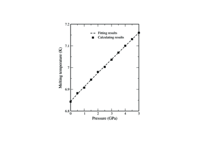
Figure 8: The melting points($T_{M}$) as a function of pressures for $Ni_{567}$. The melting temperatures is found to increase with the increasing of pressures, in agreement with the basic thermodynamics.

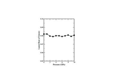
Figure 9: The latent heat versus pressure for $Ni_{561}$ cluster. The latent heat seems to be a constant in the studied range of pressures.

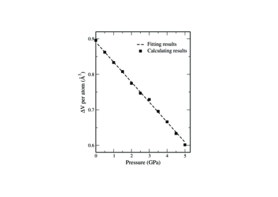
Figure 10: The volume difference between the solid state and liquid state at the melting point versus pressure for $Ni_{561}$ cluster. Dash line: deduced from Clapeyron equation, Square: from the simulation.

Fig. 8 shows the melting points($T_{M}$) as a function of pressures for $Ni_{561}$. Consistent with the basic thermodynamics, the melting temperatures is increasing with the increasing of pressures. The similar results is found for $Ni_{147}$ and bulk materials. The latent heat versus pressure for $Ni_{561}$ cluster is shown in Fig.9. From this figure, we can see that the latent heat seems to be a constant in the studied range of pressures, where the average value is about 0.0806eV. The volume difference between the solid state and liquid state at the melting point versus pressure for $Ni_{561}$ cluster shown in Fig.10. Assuming the latent heat is the constant, The melting temperature and volume difference are related through the Clapeyron equation quite well.

(b) Structure transformation of CdSe nanocrystals

Ye et al studied the structure transformation of CdSe nanocrystals using the ECPMD. The empirical potential developed by Rabani.Rabani02 has been used to describe the interatomic interaction. Most of their simulations are carried out at 300 K by using a Nosé-Hoover thermostat.NH The remarkable structure character of nanoclusters is the large surface-volume ratio, thus it can be expected that the surface could play an important role for the structure transformation in nano systems. In order to study the effect of the surface structure on the transition mechanism, they use nanocrystals of two different shapes, i.e, the spherical and faceted one, consisting of 500 to 5000 atoms. The initial configuration of the spherical nanocrystal is simply cut from the bulk CdSe of WZ structure. Faceted nanocrystals with well-defined surface structure are obtained by cleaving the bulk lattice along equivalent (100) WZ planes and at (001) and (00$\bar{1}$)planes perpendicular to the [001] direction of the $c$ axis. The volume of the nanocrystals is approximated based on finding the subset of atoms forming the smallest convex polyhedron.

Ye et al have observed the transformation from wurtzite to rocksalt structure, but the process of transformation is strongly dependent on the shape and size of the nanocrystals. Upon loading the pressure, the spherical CdSe nanocrystals is found to directly transfer to rocksalt structures with nanoscale grain boundary formed, while the faceted ones can first transfer to hexagonal MgO structure, and then the final rocksalt structure with grain boundary free. These results are similar to that calculated by the direct method for the same systems.

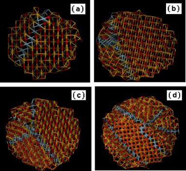
Figure 14: Domains after the structural transformation in spherical nanocrystals. (a), (b), (c) and (d) show the cross sections through the middle of the nanocrystals of radius 19 Å, 23 Å, 27 Å and 33 Å, respectively. The grain boundaries are shown with gray atoms.

Fig.11 shows their calculated the volume-pressure plot. From this figure, it clearly indicates the structural transformation of the CdSe nanocrystal up loading pressures. The volume of the spherical $Cd_{502}Se_{502}$ nanocrystal decreases smoothly with increasing pressure up to a critical pressure$\sim$ 8.0 GPa, at which the volume decreases abruptly as a result of the transformation from WZ to RS(left penal of Fig.14). This is in good agreement with the high pressure experiment for the same system.Chen97 For faceted nanocrystals, an intermediate structure(C$\rightarrow$D) clearly exists between WZ and RS. Detailed analysis of the variations of coordinations shows that the WZ structure of faceted nanocrystal transforms to a five-fold coordinated structure around 1.4GPa. The five-fold coordinated structure has been reported as a stable phase of MgO under hydrostatic tensile loading.Limpijumnong01 ; Kulkarni06 When the pressure continues to increase, the five-fold coordinated structure transforms to six-fold coordinated RS structure. The transition process is also found to be highly hysteretic. Upon pressure releasing, The rock salt structure remains stable down to pressures significantly below the observed ”upstroke” transition pressure. As low as 0.5 GPa, the sample begin to restore WZ structure. At atmospheric pressure, the WZ is recovered but with a few defects near surfaces.

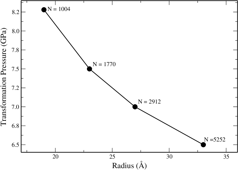
Figure 12: Variation of the transformation pressure with radius for spherical CdSe nanocrystals at 300 K. With increasing nanocrystal size, the transformation pressure decreases.

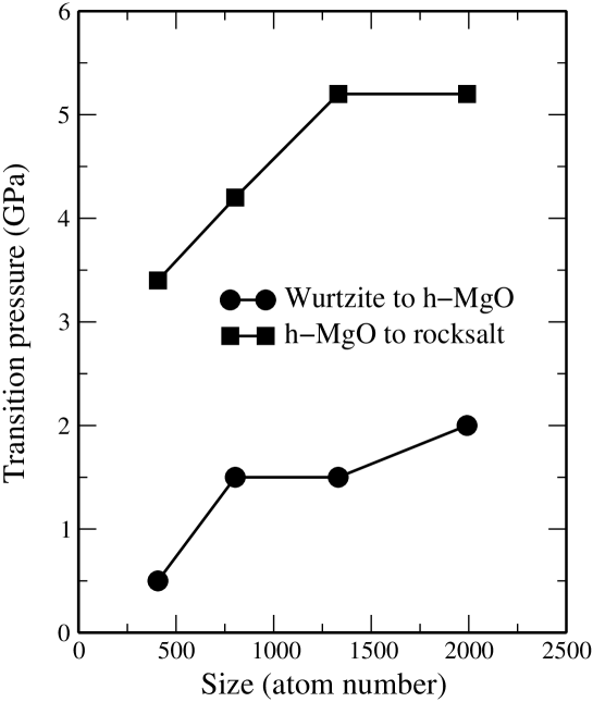
Figure 13: The transformation pressure as a function of radius for facted nanocrystals at 300 K. In contract with spherical one, the transformation pressure increases with increasing nanocrystal size.

For spherical nanocrystals, the transformation pressure decreases with size increasing. This trend coincides with the experimental results of Alivisatos.Tolbert94 ; Tolbert95 (Note, in Ye et al’s studies, ”upstroke” transition pressure is used as the transition pressure) In contrast to the spherical one, the transformation pressures (both from four-fold to five-fold and from five-fold to six-fold one) of facet nanocrystals increase with the increasing of crystal sizes. Fig. 12 and Fig.13 shows the transformation pressure as a function of sizes for facet nanocrystals. The different dependence of transformation pressure on the size has been discussed based on thermodynamics considerations by including the surface effect.

For all spherical nanocrystals, nano-scale ’grain’ boundaries are formed during and after the transformation(see Fig.14). As the size of the nanocrystal increases, the multiple grains phenomena become more and more obvious. In contrast, the facet one is almost grain boundary free. The generation of grain boundary has been discussed based on the nucleation mechanism.Ye_un

(c) Pressure induced hard-soft transition of carbon nanotubes

Gong and his co-workers have presented a detailed investigation on the behavior of carbon nanotubes under hydrostatic pressures by ECPMD.Sun04 ; Ye05 ; Ye07a In their simulation, a few single-walled carbon nanotube(SWCNT), double-walled carbon nanotubes(DWCNT) and multi-walled carbon nanotube(MWCNT) are investigated. For DWCNT, both commensurate and incommensurate one are considered. DWCNTs consisting of tubes, which has the same chirality, are typically commensurate; otherwise they are incommensurate. The volume is calculated by the minimal polyhedron method. The periodic boundary condition in the axial direction, and free boundary condition in the radial directions are used. The interaction between carbon atoms is described by a parameterized many-body potential.Te ; Br The intertube and intratube van der Waals interaction are modelled by the Lennard-Jones (LJ) potential.Girifalco56 ; Henrard99 To confirm the results of the classical molecular dynamics method, they also have repeated some calculations by ab-initio molecular dynamics method.

They found that all studied nanotubes(SWCNTs, DWCNTs and MWCNTs) undergo a pressure-induced hard-to-soft phase transition. The $hard$ phase at low pressure exhibits a typical bulk modulus of $~{}100$ GPa, while the $soft$ phase at high pressure exhibits a bulk modulus of only $\sim$1 GPa. Fig. 15 shows the pressure and the total energy as a function of reduced volume for a (10,10) nanotube at 300 K, where the energy at zero pressure is set to zero. Clearly, a transition at $\sim$1.0 GPa is observed. Below the transition, the $hard$ phase has a radial compressibility of 0.01 GPa^-1. Above the transition, the $soft$ phase has a radial compressibility about two orders of magnitude larger. The similar behavior was observed for other tubes.

After the hard-to-soft transition, the cross section of nanotubes changes from circular to elliptical shape. The evolutions of the cross-section shape, the bond length, and the bond angle with increasing pressure for a (10,10) nanotube are shown in Fig. 16. where two principal axes (long axis $a$ and short axis $b$) are used to characterize cross section. Below the transition pressure, $a$ remains almost equal to $b$, defining a circular shape( see Fig.16). Above the transition pressure, $a$ becomes larger than $b$, defining an elliptical shape. Eventually, as the long axis continues to increase and the short axis continues to decrease, the elliptical shape undergoes another transition to a dumbbell shape. Under even higher pressure, the dumbbell tube can become so flat that the spacing between the opposite side walls approaches the layer spacing in the graphite ($\sim$3.35$\AA$).

The trend of change in bond length and bond angle provides a good explanation of the hard-to-soft transition. Fig. 16(b) shows that the percentage change in bond length and bond angle increases simultaneously with increasing pressure below the transition, indicating a uniform shrinking of the circular shape under pressure. Above the transition, the bond length remains unchanged but the change of bond angle increases sharply with increasing pressure. Since it costs much more energy to change bond length than to change bond angle. Below the transition, the structural response to the external pressure is largely taken by the changing bond length of a circular shape, giving rise to a hard phase; while above the transition, the structural response to the external pressure is largely taken by the changing bond angle of an elliptical shape, giving rise to a soft phase.

The critical transition pressure depends strongly on the tube radius. Fig. 17 shows the simulated transition pressures as a function of tube radius for SWNTs(solid dots). The smaller the radius, the higher the transition pressure. To understand the above simulation results, they also provide a general analysis based on continuum elastic theory. According to their deduction, transition pressure $P_{t}$ has,

$$P_{t}\approx\frac{3D}{R_{0}^{3}},$$ (20)

where D is the constant related to the elastic properties of NTs, and $R_{0}$ is the tube radius. This analytical dependence of $P_{t}$ on $R_{0}$ is in very good agreement with the MD simulations, as shown in Fig. 17.

The bulk modulus of the hard phase follows,

$$B_{h}=\frac{C}{2R_{0}}.$$ (21)

where C is another constant related to the elastic properties of NTs. This analytical dependence of bulk modulus on $R_{0}$ are in very good agreement with the MD simulations, as shown in Fig. 17.

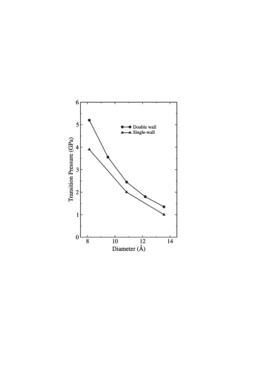
Figure 18: Transition pressure as a function of radius of nanotubes at 300 K for a few DWCNTs.

The similar pressure-induced structural transition has been found for all studied DWNT’s. Comparing with SWNT, the transition pressure of DWNT is much enhanced, but it still follows the Eq. 20. Figure 18 presents the transition pressure as a function of the both inner and outer tube radius. The results imply that the van der Waals forces between two tubes does affect the transition pressure. The transition pressure of a outer tube in DWNT can be increased largely by inserting an inner tube. In fact, the DWNT can be considered as a psudo-single-walled nanotube with effective thickness, which should be larger than the real SWNT.

The remarkable feature of MWNTs is its encapsulation effects, especially, when the system is undergoing pressure, the outer shell acts as protector for the inner shell. They found that, the response pressure of inner tube is much smaller than the external pressure, while the response pressure of outer tube is much closer to the external pressure. To characterize the pressure transmission, Ye et al define a response pressure for the tubes.Ye07a Left panel of Fig. 18 shows the response pressure as functions of external pressure of (5,5)@(10,10) DWCNT. Form this figure, on can see that the response pressure of both inner and outer tube increases linearly with the external pressure below 8 GPa, while the value for inner tube is about two times smaller than outer one. Interestingly, for all the studied tubes, when the external pressure is higher than a certain value, at which the hard-to-soft transition happens, ($\sim$8 GPa for (5,5)@(10,10) and $\sim$7 GPa for (5,5)@(10,10)@(15,15)), the response pressure of inner tube increases sharply, while increasing of the response pressure of the outer tube slows down.

Ye et al assume a linear relationship between the response pressure and the external pressure before the structural transition happens, they define pressure transmission efficiency $\beta$ by

$$P_{r}=\alpha+\beta P_{e}$$

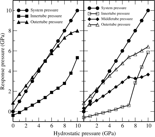
Figure 19: Response pressure as a function of the external pressure for (5,5)@(10,10) DWCNT(left) and (5,5)@(10,10)@(15,15) TWCNT(right). The system response pressure is exactly the same as the external pressure. The response pressure of inner tube is much smaller than that of the outer one before structural transition occurs.

where $P_{r}$ and $P_{e}$ are the response pressure of the inner tube and the external pressure respectively, $\alpha$ is the response pressure of the inner tube without external pressure. Fig. 19 presents the pressure transmission efficiency of (n,n)@(n+5,n+5) DWCNTs as a function of the radius of the outer tube. The pressure transmission efficiency is found to increase with the tube radius.

In contrast to commensurate DWCNTs, the incommensurate DWCNTs have lower transmission efficiency. The pressure transmission efficiency are 0.30 and 0.35 for (6,6)@(19,0) and (10,10)@(26,0) respectively, while the pressure transmission efficiency of their commensurate counterpart (6,6)@(11,11) and (10,10)@(15,15) are 0.35 and 0.43 respectively. Obviously the morphology combination does affect the vdW interaction between inner and outer tubes. The calculations show that the pressure transmission of the commensurate DWCNTs is more efficient. This might be due to the fact that the atomic positions in adjacent shells are well matched in commensurate DWCNTs, meanwhile the intralayer vdW force favors commensurate tubes.Kolmogorov00

$VI$. Summary

By writing the volume of a system as a function of coordination of atoms and extending the Lagrangian of the system to include a PV term, a constant-pressure molecular-dynamics method can be achieved in a simple but physically rigid way. This method is different the traditional constant-pressure one by treating volume as a part of potential in steady of a generalized dynamics variable. This method is specially suitable for finite systems and the system without periodic boundary conditions. In this paper, the varies of application and some technique key issues of this method are reviewed. The method is fairly general and can find widespread applications.

Figure 1: Bottom panel: The volume per atoms for liquid Ni calculated by VWS (thin line) and the exact one (thick line) obtained by traditional constant pressure molecular dynamics simulation at 3000K and 5GPa. Up panel: the same as bottom panel except the volume averaged over a short time. The two lines are close to each other

Figure 2: The evolution of the instantaneous internal pressure (middle penal), enthalpy (low penal) and volume (up penal) during ECPMD runs for $C_{60}$. The ECPMD does recover a constant pressure simulation.

Figure 3: The same as Fig.2 except the system is carbon nanotube.

Figure 4: The internal pressure as a function of external pressure for $C_{60}$ and carbon nanotube. Clearly they are equal!

Figure 5: The equations of state for Ni nanocrystals (filled circles) and bulk phase (open circles), where the data for $Ni_{3151}$ nanocrystals and bulk phase are calculated by ECPMD traditional molecular dynamics simulation respectively.

Figure 6: The bulk modulus as a function of the size of nanocrystals. Circles: calculated data, line: the linear fitting to the data.

Figure 7: The bulk modulus as a function of temperature for $Ni_{1985}$.

Figure 11: Volume versus pressure for faceted $Cd_{1162}Se_{1162}$ (right) and spherical $Cd_{502}Se_{502}$ nanocrystal (left). The discontinuity of the slopes indicates structural transformation.

Figure 15: The energy and pressure as a function of the reduced volume for (10,10) carbon nanotube at 300 K. The minimum energy is set to zero, and the volume is normalized by the equilibrium volume without the external pressure. At about 1.0 GPa, the $hard$ phase with bulk modulus of about 100 GPa transforms into the $soft$ phase with bulk modulus of just a few GPa.

Figure 16: The length of the long and short axes, as a function of pressure for (10,10) nanotube. The shape of cross section at some selected pressures is plotted at the bottom of the figure. The absolute relative change of bond length and bond angle as a function of pressure for (10,10) nanotube, the data is obtained by quenching the system from 300 K to 0 K at constant pressure.

Figure 17: The transition pressure (upper panel) and the elastic modulus (lower panel) as a function of tube radius at 300 K. The solid line is a least-square fit to the data using Eq. 20 (upper panel) and Eq. 21 (lower panel). The simulated data follows nicely with the predicted behavior.

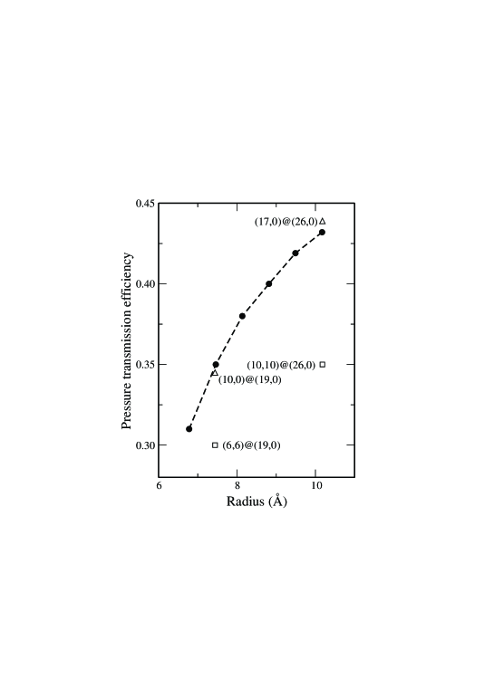
Figure 20: Pressure transmission efficiency of commensurate (n,n)@(n+5,n+5) DWCNT (with n=5,6,7,8,9,10) versus the outer tube radius. The transmission efficiency increases with the tube radius. The incommensurate DWCNTs (6,6)@(19,0) and (10,10)@(26,0) is also shown for comparison, of which the transmission efficiency is smaller.

- (1) M. P. Aleen and D. J. Tildesley, Computer Simulation of Liquid, Clarendon Press, Oxford, (1997).
- (2) H. C. Andersen, J. Chem. Phys. 72, 2384 (1980).
- (3) M. Parrinello and A. Rahman, J. Appl. Phys. 52, 7182 (1981); Phys. Rev. Lett. 45, 1196 (1980).
- (4) Proceedings of the XXXVI European High-Pressure Research Group Meeting on molecular and Low Dimensional System under pressure, Catania, Italy, 1998, edited by G. G. N. Angilella, R. Pucci, and G. Piccitto, and F. Siringo, Book of Abstracts.
- (5) F. Gradrat et al., Eur. J. Biochem, 262, 900 (1999).
- (6) S. H. Tolbert and A. P. Alivisatos, Z. Phys. D 26, 56 (1993); J. Chem. Phys. 102, 4642 (1995); Science 265, 373 (1994); Annu. Rev. Phys. Chem. 46, 595 (1995); S. H. Tolbert et al., Phys. Rev. Lett. 76, 4384 (1996).
- (7) R. Martonak, C. Molteni and M. Parrinello, Phys. Rev. Lett. 84, 682 (2000).
- (8) J. Kohanoff, A. Caro and M. W. Finnis, ChemPhysChem, 6, 1848 (2005).
- (9) D. Y. Sun and X. G. Gong, J. Phys.: Condens. Matter 14, L487 (2002); ibid, arXiv:cond-mat/0102184.
- (10) F. Calvo and J. P. K. Doye, Phys. Rev. B 69, 125414(2004).
- (11) M. Ji et al unpublished.
- (12) Y. Ye et al unpublished.
- (13) X. Ye, D. Y. Sun and X. G. Gong, to be published.
- (14) D. Y. Sun, D. J. Shu, M. Ji, Feng Liu, M. Wang, and X. G. Gong, Phys. Rev. B 70, 165417 (2004).
- (15) X. Ye, D. Y. Sun, and X. G. Gong, Phys. Rev. B 72, 035454(2005).
- (16) X. Ye, D. Y. Sun, and X. G. Gong, Phys. Rev. B 75, 073406(2007).
- (17) S. E. Baltazar, et al, Computational Materials Sciences 37, 526(2006).
- (18) P. Tangney, et al, Nano Letters 5, 2268(2005).
- (19) Michael Grünwald, Eran Rabani, and and Christoph Dellago, Phys. Rev. Lett.96, 255701 (2006).
- (20) Statistical Physics 3rd edition Part 1, L. D. Landau and E. M. Lifshitz, Pergamon Press, 1976.
- (21) M. Ji, D. Y. Sun, X. G. Gong SCIENCE IN CHINA A 47, 92 Suppl(2004)
- (22) S. Nose, J. Chem. Phys. 81, 511 (1984); W. G. Hoover, Phys. Rev. A 31, 1695 (1985).
- (23) Hai-Ping Cheng, Xinling Li, R. L. Whetten and R. S. Berry, Phys. Rev. A 46, 791 (1992).
- (24) J. P. Lu, Phys. Rev. Lett. 79, 1297 (1997).
- (25) D. Y. Sun and X. G. Gong, Phys. Rev. B 57, 4730 (1998).
- (26) C.B. Barber, D.P. Dobkin, and H. Huhdanpaa, ACM Trans. Math. Softw.22, 469 (1996).
- (27) A. P. Sutton and J. Chen, Phil. Mag. Lett. 61, 139 (1990).
- (28) J. N. Wickham, A. B. Herhold, and A. P. Alivisatos, Phys. Rev. Lett.84, 923 (2000).
- (29) S. H. Tolbert and A. P. Alivisatos, Science265, 373 (1994).
- (30) S. H. Tolbert and A. P. Alivisatos, J. Chem. Phys.102, 4642 (1995).
- (31) C.-C. Chen, A. B. Herhold, C. S. Johnson, and A. P. Alivisatos, Science276, 398 (1997).
- (32) K. Jacobs, D. Zaziski, E. C. Scher, A.B. Herhold, and A. P. Alivisatos, Science293, 1803 (2001).
- (33) K. Jacobs, J. Wickham, and A. P. Alivisatos, J. Phys. Chem. B106, 3759 (2002).
- (34) D. Zaziski, S. Prilliman, E. C. Scher, M. Casula, J. Wickham, S. M. Clark, and A. P. Alivisatos, Nano Lett.4, 943 (2004).
- (35) F. Ercolessi, M. Parrinello and E. Tosatti, Philos. Mag. A 58, 213 (1988).
- (36) Fabrizio Cleri and Vittorio Rosato, Phys. Rev. B 48, 22 (1993).
- (37) S. Limpijumnong and W. R. L. Lambrecht, Phys. Rev. Lett 86, 91 (2001).
- (38) A. J. Kulkarni, M. Zhou, K. Sarasamak, and S. Limpijumnong, Phys. Rev. Lett 96, 105502 (2006).
- (39) D. W. Brenner, Phys. Rev. B 42, 9458 (1990).
- (40) J. Tersoff, Phys. Rev. Lett. 61, 2879 (1988).
- (41) L. A. Girifalco and R. A. Lad, J. Chem. Phys. 25, 693 (1956).
- (42) L. Henrard, E. Hern ndez, P. Bernier, and A. Rubio, Phys. Rev. B 60, R8521 (1999).
- (43) A. N. Kolmogorov and V. H. Crespi, Phys. Rev. Lett. 85, 4727 (2000).
- (44) E. Rabani, J. Chem. Phys.116, 258 (2002).