Generation of Higher-Order Harmonics By Addition of a High Frequency XUV Radiation to the IR One

Abstract

The irradiation of atoms by a strong IR laser field of frequency $\omega$ results in the emission of odd-harmonics of $\omega$ (”IR harmonics”) up to some maximal cut-off frequency. The addition of an XUV field of frequency $\tilde{q}\omega$ larger than the IR cut-off frequency to the IR driver field leads to the appearance of new higher-order harmonics (”XUV harmonics”) $\tilde{q}\pm 2K,2\tilde{q}\pm(2K-1),3\tilde{q}\pm 2K,...$ ($K$ integer) which were absent in the spectra in the presence of the IR field alone. The mechanism responsible for the appearance of the XUV harmonics is analyzed analytically using a generalization of the semiclassical re-collision (three-step) model of high harmonic generation. It is shown that the emitted HHG radiation field can be written as a serie of terms, with the HHG field obtained from the three-step model in its most familiar context [P. B. Corkum, Phys. Rev. Lett. 71, 1994 (1993)] resulting from the zeroth-order term. The origin of the higher-order terms is shown to be the ac-Stark oscillations of the remaining ground electronic state which are induced by the XUV field. These terms are responsible for the appearance of the new XUV harmonics in the HGS. The XUV harmonics are formed by the same electron trajectories which form the IR harmonics and have the same emission times, but a much lower intensity than the IR harmonics, due to the small quiver amplitude of the ac-Stark oscillation. Nevertheless, this mechanism allows the extension of the cut-off in the HGS without the necessity of increasing the IR field intensity, as is verified by numerical time-dependent Schrödinger equation simulation of a Xe atom shined by a combination of IR and XUV field.

03.65.-w, 42.50.Hz, 42.65.-Ky, 32.80.Rm

Focusing intense linearly-polarized monochromatic infra-red (IR) laser pulses into gas of atoms can lead to the emission of high-energy photons with frequencies extending into the extreme ultraviolet (XUV) and X-ray region by high harmonic generation (HHG). All major features of HHG, such as its comb-like spectrum of odd-integer harmonics (to be called ”IR harmonics”), its photons’ maximal energy (to be called ”IR cut-off”) and the emission times of each harmonic, could be well reproduced using a semiclassical three-step (recollision) model P. B. Corkum ; M. Lewenstein ; K. J. Schafer : under the influence of the intense laser field the electron of an atom tunnels out of the modified Coulomb potential, gains kinetic energy as a free particle in the field and finally may recombine with the parent ion to release the sum of its kinetic energy and the ionization potential as a high energy photon. The emission times of different harmonics are perfectly synchronized with the driver field, making the HHG process a promising method for the production of an adjustable coherent X-ray source. The current method of achieving the state of the art IR cut-off positions in the harmonic generation spectra (HGS) makes use of high-intensity few-femtosecond IR laser pulses. The main drawback of this method is that the electronic plasma which is inevitably formed at such high intensities, causes large dispersion on the propagating harmonics and severely limits their phase matching. The method to achieve higher-energy harmonics which will be presented here, doesn’t suffer from this limitation, since it allows the usage of an IR source of moderate intensity which produces a small amount of plasma. It uses an XUV driving field which is shined on the atom simultaneously with the IR one. Taking the frequency of the XUV field larger than the IR-cut off frequency and inside some spectral window of the HHG generating gas, new higher order harmonics (to be called ”XUV harmonics”), which were absent in the spectra in the presence of the IR field alone, could be produced, with frequencies well above the IR cut-off frequency, while the XUV photoionization could be suppressed, thus un-altering the amount of electronic plasma. As will be shown, the main drawback of this method is that the new XUV harmonics have a relatively low intensity.

The idea of contaminating the strong IR field with a second or more higher-frequency [usually ultra-violet (UV)] fields, is not a new one in the context of strong laser-matter interactions. The effect on the dynamical behavior of the electrons is dramatic, and such two-color (bichromatic) schemes have drawn a lot of attention in recent years. The additional field, if adjusted correctly, can induce stimulated emission Ph. Zeitoun , single-photon ionization Markus Kitzler , or multi-photon ionization N. A. Papadogiannis . This ionization effect is actually utilized for attosecond (as) pulse-duration measurement, by the analysis of photoelectrons which are emitted from atoms exposed simultaneously to the as-pulses and strong IR field Hentschel . The HGS obtained using bichromatic laser fields T. Pfeifer ; T. Pfeifer+L. Gallmann ; N. Dudovich ; H. Eichmann ; M. B. Gaarde+A. L'Huillier , polychromatic fields Enrique Conejero Jarque ; M. B. Gaarde ; C. Figueira , or even as-pulses Markus Kitzler instead of the conventional monochromatic field, had been studied extensively as well. To the best of our knowledge, in all above-mentioned studies, the frequency of the UV field was in the plateau of the HGS generated by the IR field alone (to be called here ”IR HGS”), or close to its cut-off C. Liu ; K. Ishikawa . Such a UV field could only increase the efficiency of the existing IR harmonics and/or create new peaks (hyper raman lines) still in the support of the IR HGS, or maybe extend the IR cut-off to some limited extent [As will be shown here, it is the taking of the XUV field’s frequency beyond the IR-cut off that pushes the cut-off position substantially to higher frequencies]. On the basis of the three-step (re-collision) model, it had been argued that the role of the UV field is to switch the initial step in the generation of high harmonics from tunnel ionization to the more efficient single UV-photon ionization A. Heinrich , or to assist the tunneling by transferring population to an excited state, from which the tunneling rate is larger A. Bandrauk ; K. Ishikawa , especially if the UV photon energy matches some level transition K. Schiessl ; K. Ishikawa+K. Midorikawa . This might explain the improved macroscopic HHG signal obtained in experiments: the UV-assisted ionization increases the number of atoms which participate in the HHG process and improves phase matching (the possibility that the improvement in HHG efficiencies is due to the interaction of the strong IR field with the created ions was shown to be implausible C. Valentin ). The above explanation doesn’t apply, however, for the case that will be discussed in this paper, i.e. a case in which the high-frequency field in the bichromatic HHG scheme is in the XUV regime (and not in the UV one), with frequency well above the IR cut-off frequency. By choosing the frequency of the XUV field to fall inside some spectral window of the HHG generating gas, the XUV photoionization process could be eliminated (the same effect is achieved automatically for high-enough energies of the XUV photon since the single XUV photon ionization cross section scales as the $7/2$-th power of the XUV photon’s wavelength Sakurai ). Thus, in this case, the contribution of the XUV field to the generation of the XUV harmonics is not via affecting the ionization stage anymore. Another suggestion for the role that the high-frequency photons play in the HHG process was that they control the timing of ionization, and preferentially select certain quantum paths of the electron K. J. Schafer+M. B. Gaarde . While this effect may lead to the enhancement of the low-order harmonics in the plateau, it can’t account for the large enhancement in the cutoff and beyond (which is noticeable in the results in Fig.1).

A three-step model classical analysis of HHG suggests that the contribution of the XUV field to the kinetic energy of the returning electron is negligible. To see this, suppose we irradiate the atom with a linearly-polarized IR fundamental field of frequency $\omega$, amplitude $\varepsilon^{in}_{1}$ and polarization $\mathbf{e_{k}}$ ($\mathbf{E_{1}}(t)=\mathbf{e_{k}}\varepsilon^{in}_{1}\cos(\omega t)$) and an XUV field of frequency $\tilde{q}\omega$ (where $\tilde{q}$ is a large enough number) and amplitude $\varepsilon^{in}_{\tilde{q}}$ ($\mathbf{E_{\tilde{q}}}(t)=\mathbf{e_{k}}\varepsilon^{in}_{\tilde{q}}\cos(\tilde{q}\omega t)$) with the same polarization. By integrating the classical equation of motion while assuming that the electron is freed at time $t_{i}$ with zero momentum, the following expression for the momentum of the electron is obtained:

$$\mathbf{p}(t)=\mathbf{p_{1}}(t)+\mathbf{p_{\tilde{q}}}(t)$$ (1)

where $\mathbf{p_{1}}(t)$ is the momentum due to the IR field alone $\mathbf{p_{1}}(t)=\frac{e\varepsilon^{in}_{1}}{\omega}[sin(\omega t)-sin(\omega t_{i})]$ and $\mathbf{p_{\tilde{q}}}(t)$ is the momentum due to the XUV field alone $\mathbf{p_{\tilde{q}}}(t)=\frac{e\varepsilon^{in}_{\tilde{q}}}{\tilde{q}\omega}[sin(\tilde{q}\omega t)-sin(\tilde{q}\omega t_{i})]$ ($e$ and $m$ are the electron’s charge and mass, respectively). The kinetic energy with two fields simultaneously present is:

$$E_{k}(t)=\frac{p^{2}(t)}{2m}=E_{k,1}(t)+E_{k,\tilde{q}}(t)+\frac{\mathbf{p_{1}}\cdot\mathbf{p_{\tilde{q}}}}{2m}$$ (2)

where $E_{k,1}(t)=\frac{p_{1}^{2}(t)}{2m}$ and $E_{k,\tilde{q}}(t)=\frac{p_{\tilde{q}}^{2}(t)}{2m}$. Note that $E_{k,\tilde{q}}(t)\propto(\frac{\varepsilon^{in}_{\tilde{q}}}{\tilde{q}\omega})^{2}$ and that the cross-term $\frac{\mathbf{p_{1}}\cdot\mathbf{p_{\tilde{q}}}}{2m}\propto\frac{\varepsilon^{in}_{\tilde{q}}}{\tilde{q}\omega}$ are much smaller than $E_{k,1}(t)$ if $\frac{\varepsilon^{in}_{\tilde{q}}}{\tilde{q}}<\varepsilon^{in}_{1}$. Usually, a large enough value of $\tilde{q}$ will fulfill this condition, even if the IR and XUV fields have similar intensities. Thus, the additional XUV field will not affect the electron trajectories and will not contribute to their kinetic energy. For this reason the relative phase between the two fields doesn’t play a role in the HGS, which is indeed verified in both classical analysis and quantum mechanical simulations (a small $q$, however, will affect the dynamics differently T. Pfeifer ; Andiel ). In addition, assigning the electron a non-zero initial momentum to account for the photoelectric effect, will not increase its kinetic energy upon recombination. To conclude, the extension of the harmonic cutoff energy due to the inclusion of the XUV field (Fig.1), isn’t a result of an increase of the electron’s kinetic energy upon recombination.

Since the XUV field doesn’t affect the kinetic energy of the electron trajectories (second step in the re-collision model), nor does it modify the ionization step (first step in the re-collision model), it must then influence the recombination step (third step in the re-collision model) of HHG. It is the purpose of this paper to prove this hypothesis. As will be shown later, the XUV field induces periodic ac-Stark modulations to the remaining ground electronic state, with the same frequency as the XUV field. The returning electronic wavepacket recombines with this modulated ground state to emit the new XUV harmonics. The IR-HGS enhancement and the cut-off extension are a result of a single atom phenomenon, and not a macroscopic one.

The paper is organized as follows: in section II we give the numerical results of the HGS obtained using a model Hamiltonian which describes a one-dimensional Xe atom subjected to a sine-square pulse of bichromatic field of frequencies $\omega$ and $\tilde{q}\omega$, for different values of $\tilde{q}$. In section III we briefly describe the semiclassical re-collision model of HHG, as is usually applied to the monochromatic case. We then modify the re-collision model to account for possible non-trivial time-dependence of the ground electronic state, and show that this modified re-collision model successfully reproduces the results presented in section II. In section IV we suggest an experiment based on the effect we discovered and conclude.

I Xe atom driven by a two-color $(\omega,\tilde{q}\omega)$ laser field

As an illustrative numerical demonstration of the IR cut-off extension in the HGS due to the addition of an XUV field, we studied a single electron 1D Xe atom irradiated by a sine-square pulse supporting $N$ oscillations of linearly polarized light of bichromatic field, composed of an IR laser field of frequency $\omega$ and amplitude $\varepsilon^{in}_{1}$ and a high-frequency field of frequency $\tilde{q}\omega$ and amplitude $\varepsilon^{in}_{\tilde{q}}$. The following time-dependent Schrödinger equation (TDSE) was integrated using the split operator method:

$$i\hbar\frac{\partial}{\partial t}\Psi(x,t)=\biggl{\{}\frac{p_{x}^{2}}{2m}+V_{0}(x)-exsin^{2}\biggl{(}\frac{\omega t}{2N}\biggr{)}[\varepsilon^{in}_{1}\cos(\omega t)+\varepsilon^{in}_{\tilde{q}}\cos(\tilde{q}\omega t)]\biggr{\}}\Psi(x,t)$$ (3)

between the times $0<t<NT$ ($T=\frac{2\pi}{\omega}$) with atomic units ($\hbar=m=-e=1$) and with the wave function taken initially as the ground state $\phi_{1}(x)$ of the field-free model Hamiltonian of a 1D Xe atom, with the field-free effective potential $V_{0}(x)=-0.63exp(-0.1424x^{2})$. This potential supports three bound states, of which the two lowest ones mimic the two lowest electronic states of Xe, with energies $-I_{p}=-0.4451a.u.$ and $E_{2}=-0.1400a.u.$. The parameters used for the simulation were $N=50$, $\omega=0.05695a.u.$ ($\lambda=800nm$), $\varepsilon^{in}_{1}=0.035a.u.$ (corresponding to intensity of $I^{in}_{1}\simeq 4.299\cdot 10^{13}\frac{W}{cm^{2}}$), $\varepsilon^{in}_{\tilde{q}}=0.0001a.u.$ ($I^{in}_{\tilde{q}}\simeq 3.509\cdot 10^{8}W/cm^{2}$). It should be noted that in this type of simulation the Born approximation is assumed: instead of solving two coupled differential equations, one for the evolution of the electron and the other for the propagation of the electromagnetic field, the electromagnetic field is assumed to remain unchanged during the interaction with the electron, and only a Schrödinger equation of motion for the electron is solved.

In order to calculate the HGS the Larmor approximation Jackson was assumed, and the time-dependent acceleration expectation value

$$a(t)\equiv\frac{1}{m}\langle\Psi(x,t)|-\frac{dV_{0}(x)}{dx}|\Psi(x,t)\rangle+\frac{e}{m}sin^{2}\biggl{(}\frac{\omega t}{2N}\biggr{)}[\varepsilon^{in}_{1}\cos(\omega t)+\varepsilon^{in}_{\tilde{q}}\cos(\tilde{q}\omega t)]$$ (4)

which is linearly proportional to the emitted field, was analyzed. The power spectra (HGS) of emitted radiation by the oscillating electron is proportional to the modulus-square of the Fourier-transformed time-dependent acceleration expectation value:

$$\sigma(\Omega)=\frac{2e^{2}}{3c^{3}}|a(\Omega)|^{2}$$ (5)

where the acceleration in frequency space is given by the Fourier transform

$$a(\Omega)=\frac{1}{NT}\int_{0}^{NT}a(t)e^{-i\Omega t}dt$$ (6)

Fig.1 shows the HGS for different values of $\tilde{q}$ ($\tilde{q}=11$, $\tilde{q}=25$, $\tilde{q}=37\frac{9}{22}$ and $\tilde{q}=52$). The HGS in the presence of the IR field alone is also shown for comparison. Several features can be seen in the figure: The position of the IR cut-off (the cut-off of the HGS in the presence of the IR field only) is at the 15th harmonic where the maximal IR harmonic is the 29th one. When the high frequency field has a frequency still within the IR-HGS, its only influence on the HGS is to modify the IR-harmonics ($\tilde{q}=11$ in Fig.1). When the high frequency field has a frequency close to the IR cut-off, the IR-harmonics are modified, and new harmonics (above the 29th harmonic), which were not present with the IR field alone, appear ($\tilde{q}=25$ in Fig.1, which corresponds to an XUV radiation of wavelength 16nm). These new harmonics, that appear due to the addition of the XUV field only, will be termed XUV-harmonics. The position of the maximal XUV harmonic increases as the XUV frequency increases ($\tilde{q}=37\frac{9}{22}$), where it becomes apparent that the XUV harmonics appear around the frequency of the XUV field. The number of new XUV harmonics reaches a maximal one (approximately twice the number of IR harmonics) whenever the value of $\tilde{q}$ is either not odd integer or is greater than approximately twice the number of the maximal IR harmonic ($\tilde{q}=52$ in Fig.1).

In general, upon the addition of the XUV field of frequency $\tilde{q}\omega$ to the IR field of frequency $\omega$ the harmonics $\tilde{q}\pm 2K$ ($K$ integer) are either modified (if they were already present in the IR-HGS) and/or appear as new XUV harmonics. Moreover, the HGS possesses certain symmetries: with respect to its center at harmonic $\tilde{q}$, the distribution of the XUV harmonics is symmetric (i.e., for $\tilde{q}=37\frac{9}{22}$, $\sigma(33\frac{9}{22}\omega)\simeq\sigma(41\frac{9}{22}\omega)$, etc.) and upon variation of $\tilde{q}$ it shifts but remains almost invariant. The structure of the HGS of the XUV harmonics (will be called XUV-HGS from now on) consists, in principal, of two new plateau-like regions and two new cut-off-like regions. For example, for $\tilde{q}=52$ in Fig.1, the harmonics of order 38-48 and 56-66 have a ”plateau” character (constant intensity), and the harmonics 32-36 and 68-72 have a ”cut-off” character (constant phase, will be shown in Fig.5). The XUV harmonics are 10-orders of magnitude weaker than the IR harmonics.

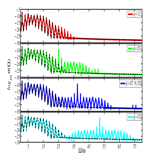
Figure 1: (color online) HGS obtained from a 1D model Hamiltonian of Xe atom (Eq.3) irradiated by a 50-oscillation sine-square pulse of bichromatic laser field composed of a 800nm IR laser field of intensity $I^{in}_{1}\simeq 4.299\cdot 10^{13}W/cm^{2}$ and a $800/\tilde{q}$-nm XUV field of intensity $I^{in}_{\tilde{q}}\simeq 3.509\cdot 10^{8}W/cm^{2}$ for different values of $\tilde{q}$: $\tilde{q}=11$ (solid red line), $\tilde{q}=25$ (solid green line), $\tilde{q}=37\frac{9}{22}$ (solid blue line) and $\tilde{q}=52$ (solid cyan line). The IR-HGS is shown as the dotted black line where the position of the IR cutoff is at the 15th harmonic. The addition of the XUV field could have several effects on the HGS, depending on its frequency with respect to the position of the IR cut-off: it could either modify the IR-HGS or slightly extend the IR cut-off ($\tilde{q}=11$), or add new XUV harmonics to the spectrum ($\tilde{q}=25,37\frac{9}{22},52$). The XUV harmonics appear at $\tilde{q}\pm 2K$, regardless of the value of $\tilde{q}$. The XUV-HGS possesses the following symmetries: with respect to its center $\tilde{q}$, the distribution of the new XUV harmonics is symmetric (i.e., for $\tilde{q}=52$, $\sigma(48\omega)\simeq\sigma(56\omega)$, etc.) and upon variation of $\tilde{q}$ it shifts but remains almost invariant.

Fig.2 shows the HGS for a larger intensity of the high-frequency field, $\varepsilon^{in}_{\tilde{q}}=0.0035a.u.$ ($I^{in}_{\tilde{q}}\simeq 4.299\cdot 10^{11}W/cm^{2}$), where all other parameters are kept the same. For sake of clarity, only two values of $\tilde{q}$ are shown $\tilde{q}=37\frac{9}{22}$ and $\tilde{q}=52$. As before, the set of new XUV harmonics $\tilde{q}\pm 2K$ ($K$ integer) appears around $\tilde{q}$. It is 7-orders of magnitude weaker than the IR harmonics. In addition, an additional set of new XUV harmonics $2\tilde{q}\pm(2K-1)$ ($K$ integer) appears around $2\tilde{q}$ and possesses the same above-mentioned symmetries: it consists of two new plateau-like regions and two cut-off-like regions. The intensity of the XUV harmonics around $2\tilde{q}$ are, however, 14-orders of magnitude weaker than the IR harmonics. A third set of XUV harmonics $3\tilde{q}\pm 2K$ appears around $3\tilde{q}$. It possesses the same above-mentioned symmetries and is 21-orders of magnitude weaker than the IR harmonics.

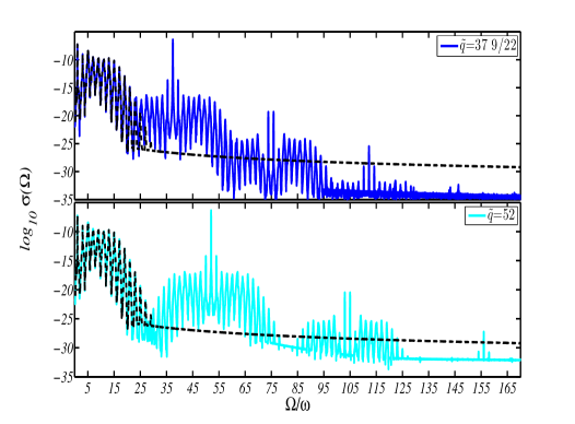
Figure 2: (color online) Same as in Fig.1, but for $I^{in}_{\tilde{q}}\simeq 4.299\cdot 10^{11}W/cm^{2}$. For $\tilde{q}=37\frac{9}{22}$ (solid blue line) three sets of XUV harmonics are observed: one at $\tilde{q}\pm 2K$, a second one at $2\tilde{q}\pm(2K-1)$, and a third one at $3\tilde{q}\pm 2K$, all differ very much in their intensities but have the same general structure and the same symmetries pointed out in Fig.1 and in the text. For $\tilde{q}=52$ (solid cyan line) only 2 sets of XUV harmonics are observed, together with traces of the third set. The constant intensity of the IR-HGS (dotted black line) above the IR cut-off should be disregarded as it is due to numerical error and could be made as low as one wishes.

For a larger intensity of the high frequency field this same trend is continued, giving rise to new sets of XUV harmonics around $4\tilde{q}\pm(2K-1)$, $5\tilde{q}\pm 2K$, etc. which could become nested but are well distinguished by the large differences in their intensities. Fig.3 and Fig.4, which show a top-view plot of the bichromatic HGS as function of $\tilde{q}$, suggest that the new sets of XUV harmonics emerge from the single set of IR harmonics. The sets of straight lines with different slopes in those plots correspond to different values of the integers $n_{1}$ and $n_{\tilde{q}}$ in the selection rules applicable for our bichromatic $(\omega,\tilde{q}\omega)$ scheme Avner Atto : the possible harmonics that could be emitted are $\Omega/\omega=n_{1}+n_{\tilde{q}}\tilde{q}$ (where $n_{1}+n_{\tilde{q}}=2K-1$), or alternatively

$$\tilde{q}=\frac{1}{n_{\tilde{q}}}\frac{\Omega}{\omega}-\frac{n_{1}}{n_{\tilde{q}}}$$ (7)

We shall symbolize the sets of lines according to their values of $n_{1}$ and $n_{\tilde{q}}$ as $(n_{1},n_{\tilde{q}})$. The set of lines parallel to the vertical axis of Fig.3 (infinite slope) correspond to $n_{\tilde{q}}=0$ and odd values of $n_{1}$, i.e. to the IR harmonics $\Omega=(2K-1)\omega$ (in a perturbative picture, this corresponds to no absorption of $\tilde{q}\omega$ photons, only an odd number of $\omega$ photons) and will be symbolized as $(n_{1},n_{\tilde{q}})=(2K-1,0)$. It is obvious that without the XUV field, only this set would appear in this type of figure. The next set of lines, with slope equal to unity, correspond to $(n_{1},n_{\tilde{q}})=(2K,1)$, i.e. to the XUV harmonics $\Omega=(\tilde{q}\pm 2K)\omega$ that are shown also in Fig.1. It is seen that these lines are much weaker than the lines corresponding to the set $(n_{1},n_{\tilde{q}})=(2K-1,0)$. The strongest line in the set $n_{\tilde{q}}=1$ corresponds to $(n_{1},n_{\tilde{q}})=(0,1)$, i.e. absorption of one $\tilde{q}\omega$ photon and no $\omega$ photons. This line, together with the lines to its right [which correspond to $(n_{1},n_{\tilde{q}})=(2,1),(4,1),...$] emerge from the same points on the function $\tilde{q}=1$ form where the IR harmonic lines emerge. The lines $(n_{1},n_{\tilde{q}})=(-2,1),(-4,1),...$ are a mirror image of the lines $(n_{1},n_{\tilde{q}})=(2,1),(4,1),...$, with respect to the central line $(n_{1},n_{\tilde{q}})=(0,1)$. This hints us that the symmetry properties of the XUV-HGS (i.e., the fact that the distribution of the XUV harmonics is symmetric with respect to $\tilde{q}$, shifts but remains almost invariant upon variation of $\tilde{q}$, and consists of two ”plateau” and two ”cut-off” regions) are the result of the fact that the XUV harmonics are ”born” from the same electronic trajectories that produce the IR harmonics. When the intensity of the high-frequency field is increased, as in Fig.4, also the sets $(n_{1},n_{\tilde{q}})=(2K-1,2)$ and $(n_{1},n_{\tilde{q}})=(2K,3)$ appear, and they are 20-orders and 30-orders of magnitude smaller than the IR harmonics, as shown in Fig.2. Also these XUV harmonics are ”born” from the electronic trajectories that produce the IR harmonics. What is the physical mechanism leading to the formation of these new sets of XUV harmonics?

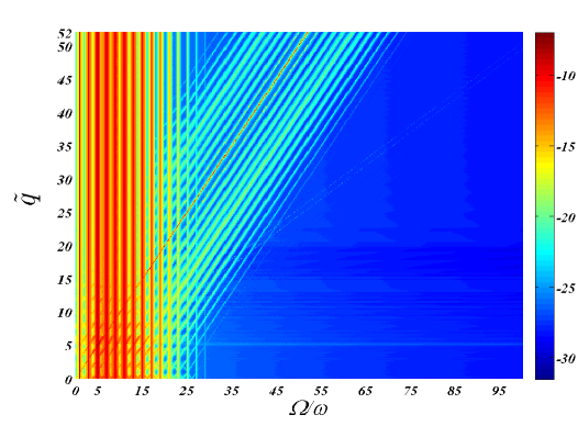
Figure 3: (color online) Top view of a log plot showing the HGS (red color-high intensity, blue color-low intensity) obtained from a 1D model Hamiltonian of Xe atom (Eq.3) irradiated by a 50-oscillation sine-square pulse of bichromatic laser field composed of a 800nm IR laser field of intensity $I^{in}_{1}\simeq 4.299\cdot 10^{13}W/cm^{2}$ and a $800/\tilde{q}$nm XUV field of intensity $I^{in}_{\tilde{q}}\simeq 3.509\cdot 10^{8}W/cm^{2}$ for different values of $\tilde{q}$. The HGS shown in Fig.1 is obtained by taking cuts of the HGS shown here along the specific values of $\tilde{q}$. The lines in the spectrum are merely a manifestation of the selection rules given in Eq.7. Groups of harmonics corresponding to absorption of more than one XUV photon are absent, due to the weak intensity of the XUV field. That is, the only set of XUV harmonics that appear is the set $\tilde{q}\pm 2K$.

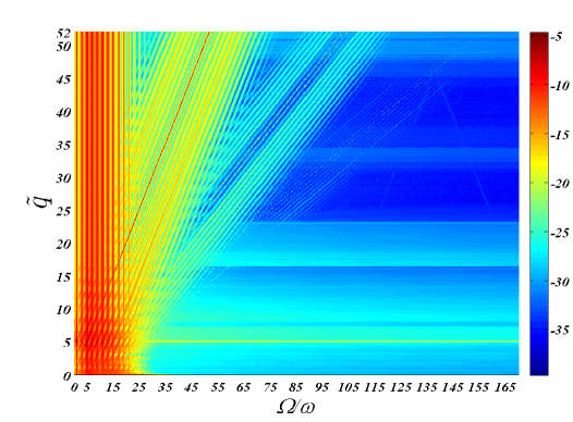
Figure 4: (color online) The same as in Fig.3 but with a larger intensity of the second field: $I^{in}_{\tilde{q}}\simeq 4.299\cdot 10^{11}W/cm^{2}$. This time, also the sets of XUV harmonics $2\tilde{q}\pm(2K-1)$ and $3\tilde{q}\pm 2K$ appear.

II The re-collision description of bichromatic $(\omega,\tilde{q}\omega)$ HHG

The process of HGS could be successfully described in terms of a very simple and intuitive model: the semiclassical re-collision model P. B. Corkum . Let us describe, for the beginning, the process of HHG driven by an IR filed only. According to this model, the electronic wavefunction at the event of recombination $\Psi(\mathbf{r},t\approx t_{r})$ could be described as a sum of the following continuum and bound parts

$$\Psi(\mathbf{r},t_{r})=\psi_{b}(\mathbf{r},t_{r})+\psi_{c}(\mathbf{r},t_{r})$$ (8)

It is assumed that the strong IR field ionizes the electron by tunneling from the initial ground state of the field-free Hamiltonian $\phi_{1}(\mathbf{r})$, which is only slightly depleted during this process. It is assumed that the electronic wavefunction which remain bound, evolves under the field-free Hamiltonian only, i.e. accumulates a trivial phase only:

$$\psi_{b}(\mathbf{r},t)=\phi_{1}(\mathbf{r})e^{\frac{i}{\hbar}I_{p}t}$$ (9)

where $-I_{p}$ is the energy of the ground state. Under the strong field approximation, the freed electronic continuum part evolves under the external field only. Taking the direction of linear polarization $\mathbf{e_{k}}$ as the x-direction from now on for simplicity, and assuming separability of the continuum wavefunction $\psi_{c}(\mathbf{r},t\approx t_{r})$ in the x-coordinate and the 2 other lateral coordinates for simplicity, the continuum wavefunction can be written as

$$\psi_{c}(\mathbf{r},t\approx t_{r})=\psi_{c}^{\parallel}(x,t\approx t_{r})\psi_{c}^{\perp}(y,z,t\approx t_{r})$$ (10)

where the returning continuum part in the direction of polarization is some superposition of plane waves

$$\psi_{c}^{\parallel}(x,t_{r})=\frac{1}{\sqrt{2\pi}}\int_{-\infty}^{\infty}dk\tilde{\psi_{c}}^{\parallel}(k,t_{r})e^{i[kx-\frac{E_{k}}{\hbar}t_{r}]}$$ (11)

where $\mathbf{k}=k\mathbf{e_{x}}$ ($k=|\mathbf{k}|$) is the momentum of the electron, $E_{k}\equiv\frac{\hbar^{2}k^{2}}{2m}$ is the usual dispersion relation and $\tilde{\psi_{c}}^{\parallel}(k,t_{r})$ are expansion coefficients which weakly depend on time.

Using the total wavefunction at the event of recombination $\Psi(\mathbf{r},t\approx t_{r})$, the time-dependent acceleration expectation value could be calculated. Keeping only the part which is responsible for the emission of radiation at frequencies other than the incident frequency $\omega$, the acceleration reads $\mathbf{a}(t)\equiv\frac{1}{m}\langle\Psi(\mathbf{r},t)|-\nabla V_{0}(\mathbf{r})|\Psi(\mathbf{r},t)\rangle_{\mathbf{r}}$, where $V_{0}(\mathbf{r})$ is the field-free potential. Assuming low depletion rate of the ground state (and hence, small population of the continuum wavepacket), the dominant terms that are responsible for the emission of radiation at frequencies other than the incident frequency $\omega$ are the bound-continuum terms

$$\mathbf{a}(t_{r})=\frac{2}{m}\Re\langle\psi_{b}(\mathbf{r},t_{r})|-\nabla V_{0}(\mathbf{r})|\psi_{c}(\mathbf{r},t_{r})\rangle_{\mathbf{r}}$$ (12)

(the bound-bound term $\langle\psi_{b}(\mathbf{r},t)|-\nabla V_{0}(\mathbf{r})|\psi_{b}(\mathbf{r},t)\rangle_{\mathbf{r}}$ is time-independent and doesn’t radiate and the contribution of the continuum-continuum term is negligible). After plugging the expressions in Eq.9-11 into Eq.12, it could be realized that the acceleration is composed of oscillating terms of the form

$$\mathbf{a}(t_{r})=\Re\int_{-\infty}^{\infty}dk\tilde{\tilde{\psi}}^{(0)}(k,t_{r})e^{-\frac{i}{\hbar}[I_{p}+\frac{\hbar^{2}k^{2}}{2m}]t_{r}}$$ (13)

where

$$\tilde{\tilde{\psi}}^{(0)}(k,t_{r})\equiv-\frac{2}{m}\frac{1}{\sqrt{2\pi}}\tilde{\psi_{c}}^{\parallel}(k,t_{r})\int_{-\infty}^{\infty}d^{3}r\phi_{1}(\mathbf{r})\nabla V_{0}(\mathbf{r})\psi_{c}^{\perp}(y,z,t_{r})e^{ikx}$$ (14)

The emitted HHG field in a single re-collision event at $t\approx t_{r}$ is a burst of light which corresponds to the spectral continuum $I_{p}<\hbar\Omega<I_{p}+3.17U_{p}$ where $3.17U_{p}\equiv 3.17\frac{e^{2}(\varepsilon^{in}_{1})^{2}}{4m\omega^{2}}$ is the value of the most energetic returning electron trajectory. In addition, since we assumed that the IR field pulls the electron along the x-direction, it is reasonable to assume symmetric evolution of the continuum wavefunction in the lateral plane, i.e., $\psi_{c}^{\perp}(y,z,t_{r})=\psi_{c}^{\perp}(-y,-z,t_{r})$. Since for atoms $V_{0}(\mathbf{r})$ and $\phi_{1}(\mathbf{r})$ are symmetric functions (and $\nabla V_{0}(\mathbf{r})$ is antisymmetric), we get from Eq.14 that the coefficient $\tilde{\tilde{\psi}}^{(0)}(k,t_{r})$ has a nonzero component along the x-direction only, i.e., the acceleration $\mathbf{a}(t_{r})$ points along the x-direction, as it should.

When each single re-collision event is repeated every half cycle of the IR field, integer odd harmonics $2K-1$ are obtained in the HGS. To see this we compare two consecutive re-collision events at times $t_{r}$ and $t_{r}+\frac{T}{2}$. Suppose we assume that $\psi_{c}^{\parallel}(x,t_{r})$ was born at some initial time $t_{i}$ from $\phi_{1}(\mathbf{r})$. Therefore, since $\psi_{c}^{\parallel}(x,t_{r}+\frac{T}{2})$ was born $\frac{T}{2}$ after $\psi_{c}^{\parallel}(x,t_{r})$, at the time $t_{i}+\frac{T}{2}$, it was born from $\phi_{1}(\mathbf{r})e^{\frac{i}{\hbar}I_{p}\frac{T}{2}}$ since the bound state from which the continuum state tunnels out, has accumulated this phase. In addition, the two continuum functions $\psi_{c}^{\parallel}(x,t_{r})$ and $\psi_{c}^{\parallel}(x,t_{r}+\frac{T}{2})$ are released in opposite spatial directions, because the IR field changes direction in two subsequent tunneling times. Therefore, the symmetry relation between $\psi_{c}^{\parallel}(x,t_{r})$ and $\psi_{c}^{\parallel}(x,t_{r}+\frac{T}{2})$ is

$$\psi_{c}^{\parallel}(x,t_{r})=\psi_{c}^{\parallel}(-x,t_{r}+\frac{T}{2})e^{-\frac{i}{\hbar}I_{p}\frac{T}{2}}$$ (15)

Plugging this symmetry into Eq.11, and using the property $E_{k}\equiv\frac{\hbar^{2}k^{2}}{2m}=E_{-k}$, we get by simple change of variables of the integral that

$$\tilde{\psi_{c}}^{\parallel}(k,t_{r})=\tilde{\psi_{c}}^{\parallel}(-k,t_{r}+T/2)e^{-\frac{i}{\hbar}(I_{p}+E_{k})\frac{T}{2}}$$ (16)

Using the relations mentioned before ($V_{0}(\mathbf{r})=V_{0}(-\mathbf{r})$, $\phi_{1}(\mathbf{r})=\phi_{1}(-\mathbf{r})$, $\nabla V_{0}(\mathbf{r})=-\nabla V_{0}(-\mathbf{r})$, $\psi_{c}^{\perp}(y,z,t_{r})=\psi_{c}^{\perp}(y,z,t_{r}+T/2)=\psi_{c}^{\perp}(-y,-z,t_{r})$) the following symmetry is obtained from Eq.14:

$$\tilde{\tilde{\psi}}^{(0)}(k,t_{r})=-\tilde{\tilde{\psi}}^{(0)}(-k,t_{r}+T/2)e^{-\frac{i}{\hbar}(I_{p}+E_{k})\frac{T}{2}}$$ (17)

Using this symmetry, we get from Eq.13 that:

$$\mathbf{a}(t_{r}+T/2)=-\mathbf{a}(t_{r})$$ (18)

The acceleration vector is periodic in $T$ and alternates directions between subsequent re-collision events, i.e., its only nonzero components in its Fourier expansion correspond to odd integer harmonics of $\omega$. This is the origin of the well-known odd selection rules of monochromatic HHG. We shall therefore symbolize the acceleration which is responsible for the emission of odd harmonics (Eq.13) as $\mathbf{a}^{(0)}(t)$.

The three-step model described above assumes that the only time evolution of the remaining bound part of the electronic wavefunction is to accumulate a trivial phase, as given in Eq.9. This assumption, however, describes only the leading term in the time evolution of the bound part. In reality, due to the ac-Stark effect induced by the IR field, the electron adiabatically follows the instantaneous ground state of the potential which periodically shakes back and forth by the IR field. If one carries out a TDSE simulation and looks at the electronic wavefunction in the field-free potential region during the action of the IR field, one sees that it oscillates back and forth with the same frequency of the IR field. The time evolution of the bound part $\psi_{b}(\mathbf{r},t)$ should be therefore corrected from the trivial one given in Eq.9. In addition, for common field intensities, the ac-Stark correction to the instantaneous ground state energy is negligible, and we may therefore assume that the instantaneous ground-state energy is almost constant ($I_{p}$). More importantly, the ac-Stark effect induces a periodic motion of the wavefunction as a whole, without deforming it. Relying on these facts, we approximate the instantaneous ground state wavefunction as

$$\psi_{b}(\mathbf{r},t)\cong\phi_{1}(x+\varepsilon_{1}^{out}\cos(\omega t),y,z)e^{+\frac{i}{\hbar}I_{p}t}$$ (19)

We have assumed the simplest time-dependence in $\psi_{b}(\mathbf{r},t)$ that would still give periodic modulations at frequency $\omega$. It should be noted that in the language of non-Hermitian quantum mechanics Reviewnimrod ; Avner Rapid this expression approximately describes the resonance Floquet state which evolves from the ground state $\phi_{1}(\mathbf{r})$ upon the switching of the IR field.

The quiver amplitude $\varepsilon_{1}^{out}$ of the spatial oscillations of the ground state is of the order of $\varepsilon_{1}^{out}=\frac{\varepsilon_{1}^{in}}{(E_{2}+I_{p})^{2}-\omega^{2}}$ (this is approximately the quiver amplitude of a an electron bound in a short-range potential of the type used here, driven by an IR field of amplitude $\varepsilon_{1}^{in}$), i.e., a tiny fraction of a Bohr radius, provided that the laser’s frequency doesn’t match some level transition. The bound part may therefore be expanded in a Taylor serie as

$$\psi_{b}(\mathbf{r},t)\cong e^{+\frac{i}{\hbar}I_{p}t}\{\phi_{1}(\mathbf{r})+\varepsilon_{1}^{out}\cos(\omega t)\frac{\partial}{\partial x}\phi_{1}(\mathbf{r})\}$$ (20)

Calculation of the time-dependent acceleration expectation value using the total wavefunction at the event of recombination $\Psi(\mathbf{r},t\approx t_{r})$ with the modified bound part $\psi_{b}(\mathbf{r},t_{r})$ given in Eq.20, and keeping again only the terms that are responsible for the emission of radiation at frequencies other than the incident frequency $\omega$ (the bound-continuum terms), yields:

$$\mathbf{a}(t_{r})=\mathbf{a}^{(0)}(t_{r})+\varepsilon_{1}^{out}\cos(\omega t_{r})\mathbf{a}^{(1)}(t_{r})$$ (21)

where $\mathbf{a}^{(0)}(t_{r})$ is given in Eq.13 and

$$\mathbf{a}^{(1)}(t_{r})=\Re\int_{-\infty}^{\infty}dk\tilde{\tilde{\psi}}^{(1)}(k,t_{r})e^{-\frac{i}{\hbar}[I_{p}+\frac{\hbar^{2}k^{2}}{2m}]t_{r}}$$ (22)

where

$$\tilde{\tilde{\psi}}^{(1)}(k,t_{r})\equiv-\frac{2}{m}\frac{1}{\sqrt{2\pi}}\tilde{\psi_{c}}^{\parallel}(k,t_{r})\int_{-\infty}^{\infty}d^{3}r\frac{\partial\phi_{1}(\mathbf{r})}{\partial x}\nabla V_{0}(\mathbf{r})\psi_{c}^{\perp}(y,z,t_{r})e^{ikx}$$ (23)

We see that the inclusion of the Stark effect contributes a new term $\varepsilon_{1}^{out}\cos(\omega t_{r})\mathbf{a}^{(1)}(t_{r})$ to the acceleration. In a single re-collision event at $t\approx t_{r}$, this term produces two bursts of light. One corresponds to the spectral continuum $I_{p}+\hbar\omega<\hbar\Omega<I_{p}+3.17U_{p}+\hbar\omega$ and the other to $I_{p}-\hbar\omega<\hbar\Omega<I_{p}+3.17U_{p}-\hbar\omega$. These bursts of light are, however, much weaker than the one which results from $\mathbf{a}^{(0)}(t_{r})$, since, as we recall, the factor $\varepsilon_{1}^{out}=\frac{\varepsilon_{1}^{in}}{(E_{2}+I_{p})^{2}-\omega^{2}}$ is small for common IR laser frequency and intensity (in the context of HHG experiments). It can be said in general that each electron trajectory (plane wave) with kinetic energy $E_{k}$, recombines with the nucleus to emit radiation of energy $I_{p}+E_{k}$, and two ”duplicate” photons with energies $I_{p}+E_{k}-\hbar\omega$ and $I_{p}+E_{k}+\hbar\omega$, at the same emission times. In a multi recollision sequence, only some of these photons will appear in the HGS, as dictated by selection rules which we are about to prove. In addition, since the functions $\frac{\partial\phi_{1}(\mathbf{r})}{\partial x}$ and $\psi_{c}^{\perp}(y,z,t_{r})$ are symmetric with respect to $y,z$ and $\nabla V_{0}(\mathbf{r})=-\nabla V_{0}(-\mathbf{r})$, we get from Eq.22-23 that the coefficient $\tilde{\tilde{\psi}}^{(1)}(k,t_{r})$ and the acceleration $\mathbf{a}^{1}(t_{r})$ point along the x-direction, as they should.

When each single re-collision event is repeated every half cycle of the IR field, the new term in the acceleration contributes integer odd harmonics $2K-1$ to the HGS. To see this we compare two consecutive re-collision events at times $t_{r}$ and $t_{r}+\frac{T}{2}$ and note that the symmetry relation between $\psi_{c}^{\parallel}(x,t_{r})$ and $\psi_{c}^{\parallel}(x,t_{r}+\frac{T}{2})$ from Eq.15 and the symmetry relation between $\tilde{\psi_{c}}^{\parallel}(k,t_{r})$ and $\tilde{\psi_{c}}^{\parallel}(k,t_{r}+\frac{T}{2})$ from Eq.16 still hold since the modification of the bound part of the electronic wavefunction has no influence on the continuum part.

Using the facts that $\frac{\partial\phi_{1}(\mathbf{r})}{\partial x}$ and $\nabla V_{0}(\mathbf{r})$ are antisymmetric with respect to inversion of $x$, the following symmetry is obtained from Eq.23:

$$\tilde{\tilde{\psi}}^{(1)}(k,t_{r})=+\tilde{\tilde{\psi}}^{(1)}(-k,t_{r}+T/2)e^{-\frac{i}{\hbar}(I_{p}+E_{k})\frac{T}{2}}$$ (24)

Using this symmetry, by calculating $\mathbf{a}^{(1)}(t_{r}+T/2)$ using the definition given in Eq.22, together with the relation given in Eq.24, we get that:

$$\mathbf{a}^{(1)}(t_{r}+T/2)=+\mathbf{a}^{(1)}(t_{r})$$ (25)

The acceleration vector $\mathbf{a}^{(1)}(t_{r})$ is periodic in $T/2$, i.e., its only nonzero components in its Fourier expansion correspond to even integer harmonics of $\omega$. The term which is responsible for the emission, $\varepsilon_{1}^{out}\cos(\omega t_{r})\mathbf{a}^{(1)}(t_{r})$, however switches signs every $T/2$, therefore giving rise to odd harmonics in the HGS ($\cos\alpha\cos\beta=\frac{1}{2}[\cos(\alpha-\beta)+\cos(\alpha+\beta)]$). That is, the radiation resulting from the ac-Stark oscillations of the bound electron is composed of odd integer harmonics of $\omega$, like the radiation which results from $\mathbf{a}^{(0)}$. The two fields, emitted by $\mathbf{a}^{(0)}$ and $\varepsilon_{1}^{out}\cos(\omega t_{r})\mathbf{a}^{(1)}$, interfere with each other in general. However, since the field resulting from $\mathbf{a}^{(1)}$ is much weaker, it is completely masked by the field produced from $\mathbf{a}^{(0)}$.

The effect of the ac-Stark oscillations on the HGS could be summarized as follows: In a single re-collision event each electron trajectory (plane wave) with kinetic energy $E_{k}$, recombines with the nucleus to emit radiation at energy $I_{p}+E_{k}$, and also, due to the ac-Stark effect, two weaker ”duplicate” electromagnetic waves with energies $I_{p}+E_{k}-\hbar\omega$ and $I_{p}+E_{k}+\hbar\omega$, at the same emission time. In a multi re-collision sequence, due to the symmetry properties discussed above, only odd-harmonic photons will appear in the HGS. The contribution to each plateau odd harmonic $\Omega$ in the HGS comes, in principle, from six emission times: the first corresponds to the recombination of the short trajectory with kinetic energy $\hbar\Omega-I_{p}$, the second corresponds to the ”duplicate” recombination resulting from a different short trajectory, with kinetic energy $\hbar\Omega-\hbar\omega-I_{p}$ (the ac-Stark oscillations of the ground state at frequency $\omega$ will make the final energy of the emitted photon $\hbar\Omega-\hbar\omega-I_{p}+\hbar\omega=\hbar\Omega-I_{p}$) and the third corresponds to the ”duplicate” recombination resulting from a different short trajectory, with kinetic energy $\hbar\Omega+\hbar\omega-I_{p}$. Three additional emission times result from three long trajectories in the same manner. Because of the large differences in intensities, usually only the two ”usual” emission times attributed to the short and long trajectories at kinetic energy $\hbar\Omega-I_{p}$ will contribute.

The effect of the ac-Stark oscillations on the HGS in this example is not large, since the harmonics produced by this mechanism are completely masked. However, high enough frequency of the ac-Stark oscillations, well above the IR cut-off, will cause the appearance of high energy photons which were not present at all in the IR HGS. In this case, the lack of contribution of the ordinary re-collision mechanism (neglecting the ac-Stark effect) to the appearance of these new high-energy photons makes the ac-Stark effect the only important one.

The way to induce ac-Stark oscillation of high frequency is by applying a second high-frequency XUV field, in addition to the IR one. The emphasis is that in order to see the new harmonics produces by the ”duplicate” trajectories due to the ac-Stark effect, the second field should be close to the IR cut-off or above, otherwise the new harmonics will be masked by the already existing IR ones.

Suppose then that we shine the atom with an IR field of frequency $\omega$ and an XUV field of frequency $\tilde{q}\omega$. As discussed before, the XUV field, provided that it has a large enough frequency, doesn’t affect the electron trajectories. Its only influence is therefore on the recombination process. This field induces ac-Stark oscillation in the exact same way as the IR field did. We may assume the same approximations used before and approximate the instantaneous ground state wavefunction as

$$\psi_{b}(\mathbf{r},t)\cong\phi_{1}(x+\varepsilon_{1}^{out}\cos(\omega t)+\varepsilon_{\tilde{q}}^{out}\cos(\tilde{q}\omega t),y,z)e^{+\frac{i}{\hbar}I_{p}t}$$ (26)

The quiver amplitude $\varepsilon_{\tilde{q}}^{out}$ of the spatial oscillations of the ground state is even smaller than $\varepsilon_{1}^{out}$ because of the high frequency of the XUV field ( $\varepsilon_{\tilde{q}}^{out}=\frac{\varepsilon_{\tilde{q}}^{in}}{(E_{2}+I_{p})^{2}-\tilde{q}^{2}\omega^{2}}\simeq\frac{\varepsilon_{\tilde{q}}^{in}}{\tilde{q}^{2}\omega^{2}}$. The bound part may be expanded in a Taylor serie as before

$$\psi_{b}(\mathbf{r},t)\cong e^{+\frac{i}{\hbar}I_{p}t}\{\phi_{1}(\mathbf{r})+[\varepsilon_{1}^{out}\cos(\omega t)+\varepsilon_{\tilde{q}}^{out}\cos(\tilde{q}\omega t)]\frac{\partial}{\partial x}\phi_{1}(\mathbf{r})\}$$ (27)

and the time-dependent acceleration expectation value is calculated using the total wavefunction at the event of recombination $\Psi(\mathbf{r},t\approx t_{r})$ with the modified bound part $\psi_{b}(\mathbf{r},t_{r})$ given in Eq.27. Keeping again only the bound-continuum terms, we get:

$$\mathbf{a}(t_{r})=\mathbf{a}^{(0)}(t_{r})+[\varepsilon_{1}^{out}\cos(\omega t_{r})+\varepsilon_{\tilde{q}}^{out}\cos(\tilde{q}\omega t_{r})]\mathbf{a}^{(1)}(t_{r})$$ (28)

where $\mathbf{a}^{(0)}(t_{r})$ is given in Eq.13 and $\mathbf{a}^{(1)}(t_{r})$ in Eq.22.

The ac-Stark effect at the frequency of the XUV field contributes a new term $\varepsilon_{\tilde{q}}^{out}\cos(\tilde{q}\omega t_{r})\mathbf{a}^{(1)}(t_{r})$ to the acceleration. In a single re-collision event at $t\approx t_{r}$, this additional term produces two bursts of light. One corresponds to the spectral continuum $I_{p}+\tilde{q}\hbar\omega<\hbar\Omega<I_{p}+3.17U_{p}+\tilde{q}\hbar\omega$ and the other to $I_{p}-\tilde{q}\hbar\omega<\hbar\Omega<I_{p}+3.17U_{p}-\tilde{q}\hbar\omega$ which, in case that the XUV field is well above the IR cut-off, could be written as $\tilde{q}\hbar\omega-I_{p}<\hbar\Omega<\tilde{q}\hbar\omega-I_{p}-3.17U_{p}$. These bursts of light are much weaker than the one which results from $\mathbf{a}_{IR}(t_{r})$, nevertheless they have a significant impact on the HGS since they are the only source of new XUV harmonics which appear now in the HGS. As explained before, each electron trajectory (plane wave) with kinetic energy $E_{k}$, recombines with the nucleus to emit radiation of energy $I_{p}+E_{k}$, and at the same time two ”duplicate” photons with energies $I_{p}+E_{k}-\tilde{q}\hbar\omega=\tilde{q}\hbar\omega-I_{p}-E_{k}$ and $I_{p}+E_{k}+\tilde{q}\hbar\omega$.

When each single re-collision event is repeated every half cycle of the IR field, the new term in the acceleration contributes to the HGS integer even harmonics around $\tilde{q}$, i.e. $\tilde{q}\pm 2K$. To see this we compare two consecutive re-collision events at times $t_{r}$ and $t_{r}+\frac{T}{2}$ and note that the result obtained in Eq.25 still holds here: $\mathbf{a}^{(1)}(t_{r}+T/2)=+\mathbf{a}^{(1)}(t_{r})$. The acceleration vector $\mathbf{a}^{(1)}(t_{r})$ is periodic in $T/2$, i.e., contributes even integer harmonics of $\omega$. The term which is responsible for the emission, $\varepsilon_{\tilde{q}}^{out}\cos(\tilde{q}\omega t_{r})\mathbf{a}^{(1)}(t_{r})$ therefore gives rise to the appearance of the harmonics $\Omega=(\tilde{q}\pm 2K)\omega$ in the HGS ($\cos\alpha\cos\beta=\frac{1}{2}[\cos(\alpha-\beta)+\cos(\alpha+\beta)]$). That is, the radiation resulting from the ac-Stark oscillations of the bound electron is composed of even integer harmonics of $\omega$ around the harmonic $\tilde{q}$. This field is much weaker than the harmonics produced by $\mathbf{a}^{(0)}$. In case that $\tilde{q}$ is an odd integer, the term $\varepsilon_{\tilde{q}}^{out}\cos(\tilde{q}\omega t_{r})\mathbf{a}^{(1)}(t_{r})$ will produce odd harmonics, which will be masked by the IR harmonics produced from $\mathbf{a}^{(0)}$, provided that $\tilde{q}$ is well below the IR cut-off harmonic. However, in case that $\tilde{q}$ is close to or above the IR cut-off harmonic or is not an odd integer, new harmonics (defined before as ”XUV harmonics”), which were not present in the HGS in the presence of the IR field alone, will appear. These harmonics will be $|\varepsilon_{\tilde{q}}^{out}|^{2}\simeq(\frac{\varepsilon_{\tilde{q}}^{in}}{\tilde{q}^{2}\omega^{2}})^{2}$-times weaker than the IR harmonics, and could therefore be distinguished from the IR harmonics by their intensity. Since these harmonics are originated by the same electronic trajectories which produce the IR harmonics, their emission times are correlated with the ones of the IR harmonics. In a single re-collision event each electron trajectory (plane wave) with kinetic energy $E_{k}$, recombines with the nucleus to emit radiation at energy $I_{p}+E_{k}$, and also, due to the ac-Stark effect, two weaker ”duplicate” electromagnetic waves with energies $I_{p}+E_{k}-\tilde{q}\hbar\omega$ and $I_{p}+E_{k}+\tilde{q}\hbar\omega$, at the same emission time. This correlation is kept also in the multi re-collision process and is manifested in the HGS: the structure (amplitude and phase) of the XUV harmonics (XUV-HGS) $\Omega=(\tilde{q}\pm 2K)\omega$ is derived from the structure of the IR-HGS. This is true for every value of $\tilde{q}$ but could be most easily seen if $\tilde{q}$ is well above the IR cut-off harmonic, since in this case the XUV harmonics are separated and are not nested in the IR-HGS. If we look at the case $\tilde{q}=52$ in Fig.1, we see that the structure of the XUV-HGS between the orders $54$ and $74$ resembles the structure of the IR-HGS between the orders 1 and 21 ($54-52-1=1$ , $74-52-1=21$). In addition, within the XUV-HGS, the structure of harmonics between the orders $32$ and $50$ is a mirror-image (with respect to the $52$-nd harmonics) of the structure of harmonics between the orders $54$ and $72$. That is, the XUV-HGS consists of two new plateau-like regions (harmonics of order 38-50 and 54-66), derived from the same electronic trajectories which form the IR-HGS plateau (harmonics of order 1-15), and two new cut-off-like regions (harmonics of order 32-36 and 68-74), derived from the same electronic trajectories which form the IR-HGS cut-off harmonics (harmonics of order 17-23). This structure of the XUV-HGS is invariant to the value of $\tilde{q}$.

What happens if we now take higher-order terms in the Taylor serie expansion of the ground state wavefunction in Eq.26? Suppose we take also the second-order term in the Taylor serie and expand the bound state according to

$$\psi_{b}(\mathbf{r},t)\cong e^{+\frac{i}{\hbar}I_{p}t}\{\phi_{1}(\mathbf{r})+[\varepsilon_{1}^{out}\cos(\omega t)+\varepsilon_{\tilde{q}}^{out}\cos(\tilde{q}\omega t)]\frac{\partial}{\partial x}\phi_{1}(\mathbf{r})+[\varepsilon_{1}^{out}\cos(\omega t)+\varepsilon_{\tilde{q}}^{out}\cos(\tilde{q}\omega t)]^{2}\frac{1}{2}\frac{\partial^{2}}{\partial x^{2}}\phi_{1}(\mathbf{r})\}$$ (29)

The time-dependent acceleration expectation value, keeping again only the bound-continuum terms, would read:

$$\mathbf{a}(t_{r})=\mathbf{a}^{(0)}(t_{r})+[\varepsilon_{1}^{out}\cos(\omega t_{r})+\varepsilon_{\tilde{q}}^{out}\cos(\tilde{q}\omega t_{r})]\mathbf{a}^{(1)}(t_{r})+[\varepsilon_{1}^{out}\cos(\omega t_{r})+\varepsilon_{\tilde{q}}^{out}\cos(\tilde{q}\omega t_{r})]^{2}\mathbf{a}^{(2)}(t_{r})$$

$$=\mathbf{a}^{(0)}(t_{r})+[\varepsilon_{1}^{out}\cos(\omega t_{r})+\varepsilon_{\tilde{q}}^{out}\cos(\tilde{q}\omega t_{r})]\mathbf{a}^{(1)}(t_{r})$$

$$+\biggl{\{}(\varepsilon_{1}^{out})^{2}\biggl{[}\frac{1+\cos(2\omega t_{r})}{2}\biggr{]}+\frac{1}{2}\varepsilon_{1}^{out}\varepsilon_{\tilde{q}}^{out}\biggl{[}\cos[(\tilde{q}+1)\omega t_{r}]+\cos[(\tilde{q}-1)\omega t_{r}]\biggr{]}+(\varepsilon_{\tilde{q}}^{out})^{2}\biggl{[}\frac{1+\cos(2\tilde{q}\omega t_{r})}{2}\biggr{]}\biggr{\}}\mathbf{a}^{(2)}(t_{r})$$

$$=\mathbf{a}^{(0)}(t_{r})+[\varepsilon_{1}^{out}\cos(\omega t_{r})+\varepsilon_{\tilde{q}}^{out}\cos(\tilde{q}\omega t_{r})]\mathbf{a}^{(1)}(t_{r})$$

$$+\biggl{\{}\frac{(\varepsilon_{1}^{out})^{2}+(\varepsilon_{\tilde{q}}^{out})^{2}}{2}+\frac{(\varepsilon_{1}^{out})^{2}}{2}\cos(2\omega t_{r})+\frac{\varepsilon_{1}^{out}\varepsilon_{\tilde{q}}^{out}}{2}\cos[(\tilde{q}+1)\omega t_{r}]+\frac{\varepsilon_{1}^{out}\varepsilon_{\tilde{q}}^{out}}{2}\cos[(\tilde{q}-1)\omega t_{r}]+\frac{(\varepsilon_{\tilde{q}}^{out})^{2}}{2}\cos(2\tilde{q}\omega t_{r})\biggr{\}}\mathbf{a}^{(2)}(t_{r})$$ (30)

where $\mathbf{a}^{(0)}(t_{r})$ is given in Eq.13, $\mathbf{a}^{(1)}(t_{r})$ in Eq.22, and $\mathbf{a}^{(2)}(t_{r})$ is

$$\mathbf{a}^{(2)}(t_{r})=\Re\int_{-\infty}^{\infty}dk\tilde{\tilde{\psi}}^{(2)}(k,t_{r})e^{-\frac{i}{\hbar}[I_{p}+\frac{\hbar^{2}k^{2}}{2m}]t_{r}}$$ (31)

where

$$\tilde{\tilde{\psi}}^{(2)}(k,t_{r})\equiv-\frac{1}{m}\frac{1}{\sqrt{2\pi}}\tilde{\psi_{c}}^{\parallel}(k,t_{r})\int_{-\infty}^{\infty}d^{3}r\frac{\partial^{2}\phi_{1}(\mathbf{r})}{\partial x^{2}}\nabla V_{0}(\mathbf{r})\psi_{c}^{\perp}(y,z,t_{r})e^{ikx}$$ (32)

The new term $+[\varepsilon_{1}^{out}\cos(\omega t_{r})+\varepsilon_{\tilde{q}}^{out}\cos(\tilde{q}\omega t_{r})]^{2}\mathbf{a}^{(2)}(t_{r})$, which results from the inclusion of the second-order term in the Taylor serie expansion of the bound wavefunction, produces 10 weaker ”duplicate” bursts of light in a single recollision event at $t\approx t_{r}$. This is due to the fact that the term multiplying $\mathbf{a}^{(2)}(t_{r})$ has 5 different frequency components. These bursts of light are much weaker than the one which results from $\mathbf{a}^{(0)}(t_{r})$ or $+[\varepsilon_{1}^{out}\cos(\omega t_{r})+\varepsilon_{\tilde{q}}^{out}\cos(\tilde{q}\omega t_{r})]\mathbf{a}^{(1)}(t_{r})$. Nevertheless, it will be shown immediately that the last two bursts (resulting from $\frac{(\varepsilon_{\tilde{q}}^{out})^{2}}{2}\cos(2\tilde{q}\omega t_{r})\mathbf{a}^{(2)}(t_{r})$) have a significant impact on the HGS since they are the only source of new XUV harmonics which appear around the harmonic $2\tilde{q}$.

Let us analyze now what happens when each single re-collision event is repeated every half cycle of the IR field. It was shown in Eq.18 that the term $\mathbf{a}^{(0)}(t_{r})$ contributes odd harmonics $\Omega=(2K-1)\omega$ to the HGS. From Eq.25 the term $\varepsilon_{1}^{out}\cos(\omega t_{r})\mathbf{a}^{(1)}(t_{r})$ also contributes odd harmonics $\Omega=(2K-1)\omega$ (with relative amplitude of the electric field of $\varepsilon_{1}^{out}$) but the term $\varepsilon_{\tilde{q}}^{out}\cos(\tilde{q}\omega t_{r})\mathbf{a}^{(1)}(t_{r})$ contributes the XUV harmonics $\Omega=(\tilde{q}\pm 2K)\omega$. Under the assumption that $\phi_{1}(\mathbf{r})$ is symmetric, $\frac{\partial^{2}\phi_{1}(\mathbf{r})}{\partial x^{2}}$ is also symmetric. Therefore, in complete analogy to what was shown in Eq.18, it can be shown that the term $\mathbf{a}^{(2)}(t_{r})$ contributes odd harmonics of $\omega$ since in two consecutive re-collision events at times $t_{r}$ and $t_{r}+\frac{T}{2}$ the following symmetry holds:

$$\mathbf{a}^{(2)}(t_{r}+T/2)=-\mathbf{a}^{(2)}(t_{r})$$ (33)

The term which is responsible for the emission, $[\varepsilon_{1}^{out}\cos(\omega t_{r})+\varepsilon_{\tilde{q}}^{out}\cos(\tilde{q}\omega t_{r})]^{2}\mathbf{a}^{(2)}(t_{r})$ therefore gives rise to the appearance of the following five sets of harmonics (with the amplitudes given in parentheses): $\Omega=[0\pm(2K-1)]\omega=(2K-1)\omega$ [$(\varepsilon_{1}^{out})^{2}+(\varepsilon_{\tilde{q}}^{out})^{2}$], $\Omega=[2\pm(2K-1)]\omega=(2K-1)\omega$ [$(\varepsilon_{1}^{out})^{2}$], $\Omega=[\tilde{q}+1\pm(2K-1)]\omega=(\tilde{q}\pm 2K)\omega$ [$\varepsilon_{1}^{out}\varepsilon_{\tilde{q}}^{out}$], $\Omega=[\tilde{q}-1\pm(2K-1)]\omega=(\tilde{q}\pm 2K)\omega$ [$\varepsilon_{1}^{out}\varepsilon_{\tilde{q}}^{out}$], $\Omega=[2\tilde{q}\pm(2K-1)]\omega$ [$(\varepsilon_{\tilde{q}}^{out})^{2}$]. Out of these five sets, the first four contribute harmonics which are masked, due to their low intensity, by IR harmonics or by the XUV harmonics resulting from the lower-order term $\varepsilon_{\tilde{q}}^{out}\cos(\tilde{q}\omega t_{r})\mathbf{a}^{(1)}(t_{r})$. The fifth set, however, contribute a new set of harmonics: $\Omega=[2\tilde{q}\pm(2K-1)]\omega$. This set is $|(\varepsilon_{\tilde{q}}^{out})^{2}|^{2}\simeq(\frac{\varepsilon_{\tilde{q}}^{in}}{\tilde{q}^{2}\omega^{2}})^{4}$-times weaker than the IR harmonics, or $|\varepsilon_{\tilde{q}}^{out}|^{2}$-times weaker than the set $\Omega=(\tilde{q}\pm 2K)\omega$ of XUV harmonics and could therefore be distinguished from these set of harmonics by their intensity. As before, these harmonics are originated by the same electronic trajectories which produce the IR harmonics, and their emission times are correlated with the ones of the IR harmonics. This is manifested in the HGS: the structure (amplitude and phase) of the new set of XUV harmonics $\Omega=[2\tilde{q}\pm(2K-1)]\omega$ in the XUV-HGS is derived from the structure of the IR-HGS. It consists, like the set $\Omega=(\tilde{q}\pm 2K)\omega$, of two new plateau-like regions, derived from the same electronic trajectories which form the IR-HGS plateau, and two new cut-off-like regions, derived from the same electronic trajectories which form the IR-HGS cut-off harmonics. This structure of the XUV-HGS is almost invariant to the value of $\tilde{q}$, as can be easily seen from Fig.2.

By generalizing the procedure described before and taking higher-order terms in the Taylor serie expansion of the bound wavefunction, it is apparent that the n-th order term contributes a new set of XUV harmonics $\Omega=[n\tilde{q}\pm(2K-1+mod(n,2))]\omega$ which is $|(\varepsilon_{\tilde{q}}^{out})^{n}|^{2}\simeq(\frac{\varepsilon_{\tilde{q}}^{in}}{\tilde{q}^{2}\omega^{2}})^{2n}$-times weaker than the IR harmonics. Note that indeed in Fig.2 for $\tilde{q}=52$, the intensity of the plateau harmonics of the set $\Omega=(\tilde{q}\pm 2K)\omega$ is indeed $|\varepsilon_{\tilde{q}}^{out})|^{2}\simeq(\frac{\varepsilon_{\tilde{q}}^{in}}{\tilde{q}^{2}\omega^{2}})^{2}=(\frac{0.0035}{52^{2}0.05695^{2}})^{2}\simeq 1.6\cdot 10^{-7}$-times weaker than the IR plateau harmonics, and the intensity of the plateau harmonics of the set $\Omega=[2\tilde{q}\pm(2K-1)]\omega$ is indeed $|\varepsilon_{\tilde{q}}^{out})|^{4}\simeq 2.5\cdot 10^{-14}$-times weaker than the IR plateau harmonics, in agreement with our theory. Fig.5, which plots the intensity of different harmonics as function of the amplitude $\varepsilon_{\tilde{q}}^{in}$ of the XUV driver field, shows indeed that the intensity of harmonics from the set $\Omega=(\tilde{q}\pm 2K)\omega$ scale quadratically with $\varepsilon_{\tilde{q}}^{in}$, while harmonics from the set $\Omega=[2\tilde{q}\pm(2K-1)]\omega$ scale as $(\varepsilon_{\tilde{q}}^{in})^{4}$. The obtained sets of XUV harmonics $\Omega=[n\tilde{q}\pm(2K-1+mod(n,2))]\omega$ are exactly as predicted by the selection-rules given in Eq.7. Hence, the inclusion of higher-order terms in the Taylor serie expansion of the bound wavefunction, leads to the generalization of the semiclassical three-step model. This allows us to obtain the selection rules for the high harmonics which are obtained upon the addition of an XUV field to an IR one, which are in complete agreement with the ones obtained using Floquet theory Avner Atto . Moreover, the intensities of the XUV harmonics can also be quantified.

Figure 5: (color online) log-log plot of the intensity of different harmonics $\sigma(\Omega)$ [$\Omega=60$ (solid red line), $\Omega=74$ (dashed green line), $\Omega=89$ (dash-dotted blue line), $\Omega=97$ (dotted cyan line)] obtained from the 1D model Hamiltonian of Xe atom (Eq.3) irradiated by a 50-oscillation sine-square pulse of bichromatic laser field composed of a 800nm IR laser field of intensity $I^{in}_{1}\simeq 4.299\cdot 10^{13}W/cm^{2}$ and a $800/52-$nm XUV field, as function of the XUV field’s amplitude $\varepsilon^{in}_{52}$. This intensity varies between $0.005a.u.$ ($I^{in}_{52}\simeq 8.773\cdot 10^{11}W/cm^{2}$) and $0.007a.u.$ ($I^{in}_{52}\simeq 1.719\cdot 10^{12}W/cm^{2}$). All 4 graphs are linear. According to the lower frame of Fig.2 ($\tilde{q}=52$), the harmonics $\Omega=60$ and $\Omega=74$ belong to the set $\tilde{q}\pm 2K$ of XUV harmonics, and as such should depend on $\varepsilon^{in}_{52}$ as $\sigma(\Omega=\tilde{q}\pm 2K)\propto(\varepsilon^{in}_{52})^{2}$ (see Eq.28). Indeed the slopes of the graphs corresponding to $\Omega=60$ and $\Omega=74$ are $2.000$ and $2.0001$, respectively. The harmonics $\Omega=89$ and $\Omega=97$ belong to the set $2\tilde{q}\pm(2K-1)$ of XUV harmonics, and as such should depend on $\varepsilon^{in}_{52}$ as $\sigma[\Omega=2\tilde{q}\pm(2K-1)]\propto(\varepsilon^{in}_{52})^{4}$ (see Eq.30). Indeed the slopes of the graphs corresponding to $\Omega=89$ and $\Omega=97$ are $4.0045$ and $4.0015$, respectively. This check confirms the correctness of our theory in this range of parameters.

The above theory predicts that both the IR and the XUV harmonics are emitted by the same IR trajectories and are therefore correlated in their emission times. This could be easily verified by plotting the time-frequency distribution of high harmonics, i.e., by analyzing the Gabor-transform (windowed Fourier transform) of the acceleration instead of the Fourier transform:

$$G_{a}(\Omega,t_{0})=\frac{1}{NT}\int_{0}^{NT}a(t)e^{-\frac{(t-t_{0})^{2}}{\tau^{2}}}e^{-i\Omega t}dt$$ (34)

where $\tau$ is the window’s width. This analysis yields a mixed time-frequency signal, i.e., not only the frequency components appearing in the acceleration but also their time of appearance $t_{0}$. Fig.6 shows the time-frequency distribution of high harmonics $(\sigma(\Omega,t_{0})\equiv\frac{2e^{2}}{3c^{3}}|G_{a}(\Omega,t_{0})|^{2})$ obtained from the time-dependent acceleration expectation value whose spectra is given in Fig.2 for $\tilde{q}=52$, for the times $26T<t<27.5T$. In accordance with the semiclassical re-collision model, different harmonics are emitted repeatedly every half cycle. In accordance with the theory developed here, the time-frequency distribution of the new sets of XUV harmonics matches the one of the IR harmonics, including the reflection symmetry of these sets (around $\tilde{q},2\tilde{q}...$). The most visible demonstration of this property is shown for the IR cut-off harmonics (the 15th-29th harmonic), who are emitted at times $t\simeq 0.710T+0.5nT$, in accordance with the semiclassical re-collision model. At those instants, also the 32nd-36th and the 68th-74th harmonics, which are the XUV cut-off harmonics of the set $\tilde{q}\pm 2K$, and also the 85th-87th and the 121st-125th harmonics, which are the XUV cut-off harmonics of the set $2\tilde{q}\pm(2K-1)$, are emitted. They are hence produced by the IR cut-off trajectories.

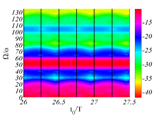
Figure 6: (Color online) Top view [pink (dark gray) color high intensity, yellow (bright gray) color low intensity] of the absolute square of the Gabor-tansformed acceleration expectation value ( Eq.34, $\tau=0.1T$) of the quantum mechanical simulation described in Fig.2 for $\tilde{q}=52$, as function of $t_{0}$ and $\Omega$.

III Suggested Experiment and Conclusions

The mechanism described here raises the question whether XUV harmonics should be self-produced in any monochromatic HHG experiment, as high-harmonic radiation generated by the leading edge of the IR pulse, co-propagates with the IR field to form a bichromatic driver field in the last part of the medium. The answer is that the high-harmonic radiation generated in the medium is too weak to considerably modify the IR-HGS. If, on the other hand, a stronger high-frequency source is used, and in particular with frequency higher than the IR cut-off frequency, new XUV harmonics should appear. This source could be a free-electron laser, but could also be a HHG-based source. Generation of HHG pulses of the 27th harmonic of Ti:sapphire laser, with width of 30fs and output energy of $0.33\mu J$ per pulse, has been shown to be feasible in Ar Takahashi . When such an harmonic pulse is focused to an area of $(10\mu m)^{2}$, intensities of $I^{in}_{27}\simeq 10^{13}W/cm^{2}$ may be reached. It isn’t unreasonable to assume that higher-harmonics couldn’t be generated with similar output energies. Even a reduction of 5 orders of magnitude in the intensity of the high-harmonic field will make the effect still visible. For example, by generating the 45th harmonic in Xe or He, filtering it out of the HGS and focusing it into a jet of Kr together with an IR field that is sufficient to generate IR cut-off at the 19th harmonic or so, new high harmonics should appear. Kr has a spectral window between photon energies of $50eV$ (the 31st harmonic) and $90eV$ (the 57th harmonic). Therefore, shining a 45th-harmonic field on it will not cause single-XUV photon ionization and will cause the appearance of new XUV harmonics in this spectral window, without the necessity to increase the intensity of the IR field.

Alternatively, in case that the frequency of the high-harmonic field isn’t large enough, one can reduce the intensity of the IR field in order to decrease the IR cut-off. The key point here is that in order to see the effect of appearance of new XUV harmonics the XUV field should be strong enough and of frequency higher than the IR cut-off frequency. Above all, the gas in which the bichromatic HHG is generated, should be transparent in some spectral band around the frequency of the XUV field, otherwise the generated XUV harmonics and/or the seed XUV field will be absorbed.

In conclusion, we have shown that the addition of an XUV field to a strong IR field leads to the appearance of new harmonics in the HGS. The results of the semiclassical analysis and the quantum numerical simulations suggest that this is a single-atom phenomena. The XUV field induces ac-Stark modulations on the ground state and affects the recombination process of all returning trajectories, and leads to the generation of higher harmonics whose emission times and intensities are well related to the ones of the harmonics in the presence of the IR field alone. Using this mechanism, harmonics with unprecedented high frequencies could be obtained in HHG experiments. According to our mechanism, the emitted HHG radiation field could be written as a serie of terms, with the zeroth-order term equal the HHG field which is obtained from the three-step model in its most familiar context P. B. Corkum . The higher-order terms become important when, in addition to the IR field, an additional XUV field is shined on the atom since they solely are responsible for the appearance of new harmonics in the HGS.

This work was supported in part by the by the Israel Science Foundation and by the Fund of promotion of research at the Technion. We thank the second referee of Avner Rapid whose comments triggered us to develop the mechanism described in this paper.

References

- [1] P. B. Corkum, Phys. Rev. Lett. 71, 1994 (1993).
- [2] M. Lewenstein, P. Balcou, M. Y. Ivanov, A. L’Huillier and P. B. Corkum, Phys. Rev. A 49, 2117 (1994).
- [3] K. J. Schafer, B. Yang, L. F. DiMauro and K. C. Kulander, Phys. Rev. Lett. 70, 1599 (1993).
- [4] Ph. Zeitoun, G. Faivre, S. Sebban, T. Mocek, A. Hallou, M. Fajardo, D. Aubert, Ph. Balcou, F. Burgy, D. Douillet, S. Kazamias, G. de Lachze-Murel, T. Lefrou, S. le Pape, P. Mercre, H. Merdji, A. S. Morlens, J. P. Rousseau and C. Valentin, Nature 431, 426 (2004).
- [5] M. Kitzler, N. Milosevic, A. Scrinzi, F. Krausz and T. Brabec, Phys. Rev. Lett, 88, 173904 (2002).
- [6] N. A. Papadogiannis, L. A. A. Nikolopoulos, D. Charalambidis, G. D. Tsakiris, P. Tzallas and K. Witte, Phys. Rev. Lett, 90, 133902 (2003).
- [7] M. Hentschel, R. Kienberger, Ch. Spielmann, G. A. Reider, N. Milosevic, T. Brabec, P. Corkum, U. Heinzmann, M. Drescher and F. Krausz, Nature 414, 509 (2001).
- [8] T. Pfeifer, L. Gallmann, M. J. Abel, P. M. Nagel, D. M. Neumark and S. R. Leone, Phys. Rev. Lett. 97, 163901 (2006).
- [9] T. Pfeifer, L. Gallmann, M. J. Abel, D. M. Neumark and S. R. Leone, Optics Letters 31, 975 (2006).
- [10] N. Dudovich, O. Smirnova, J. Levesque, Y. Mairesse, M. Y. Ivanov, D. M. Villeneuve and P. B. Corkum,Nature Physics 2, 781 (2006).
- [11] H. Eichman, S. Meyer, K. Riepl, C. Momma and B. Wellegehausen, Phys. Rev. A, 50, R2834 (1994).
- [12] M. B. Gaarde, A. L’Huillier and Maciej Lewenstein, Phys. Rev. A 54, 4236 (1996).
- [13] E. C. Jarque and Luis Roso, Optics Express 14, 4998 (2006).
- [14] M. B. Gaarde, K. J. Schafer, A. Heinrich, J. Biegert and U. Keller, Phys. Rev. A 72, 013411 (2005).
- [15] C. Figueira de Morisson Faria and M. L. Du, Phys. Rev. A 64, 023415 (2001).
- [16] Chengpu Liu, Shangqing Gong, Ruxin Li and Zhizhan Xu, Phys. Rev. A 69, 023406 (2004).
- [17] Kenichi Ishikawa, Phys. Rev. Lett. 91, 043002 (2003); Phys. Rev. A 70, 013412 (2004)
- [18] A. Heinrich, W. Kornelis, M. P. Anscombe, C. P. Hauri, P. Schlup, J. Biegert and U. Keller J. Phys. B. 39, S275 (2006).
- [19] A. D. Bandrauk and N. H. Shon, Phys. Rev. A 66, 031401R (2002).
- [20] K. Schiessl, E. Persson, A. Scrinzi and J. Burgdörfer, Phys. Rev. A 74, 053412 (2006).
- [21] Kenichi Ishikawa and Katsumi Midorikawa, Phys. Rev. A 65, 031403R (2002).
- [22] C. Valentin, S. Kazamias, D. Douillet, G. Grillon, Th. Lefrou, F. Aug, M. Lewenstein, J-F Wyart, S. Sebban and Ph. Balcou J. Phys. B. 37, 2661 (2004).
- [23] J. J. Sakurai, ”Modern Quantum Mechanics”, Revised ed. (Addison-Wesley, 1994), p. 341.
- [24] K. J. Schafer, M. B. Gaarde, A. Heinrich, J. Biegert and U. Keller, Phys. Rev. Lett. 92, 023003 (2004).
- [25] U. Andiel, G. D. Tsakiris,E. Cormier, and K. Witte, Europhys. Lett. 47, 42 (1999).
- [26] J. D. Jackson, ”Classical Electrodynamics”, 3rd ed. (John Wiley & Sons, New-York, 1975), p. 665.
- [27] A. Fleischer and N. Moiseyev, Phys. Rev. A, 74, 053806 (2006).
- [28] N. Moiseyev, Physics Reports 302, 211-293 (1998).
- [29] E. Takahashi, Y. Nabekawa, T. Otsuka, M. Obara and K. Midorikawa, Phys. Rev. A, 66, 021802 (2002).
- [30] A. Fleischer and N. Moiseyev, Phys. Rev. A, 77, 010102(R) (2008).