Fourier series and approximation on hexagonal and triangular domains

Abstract.

Several problems on Fourier series and trigonometric approximation on a hexagon and a triangle are studied. The results include Abel and Cesàro summability of Fourier series, degree of approximation and best approximation by trigonometric functions, both direct and inverse theorems. One of the objective of this study is to demonstrate that Fourier series on spectral sets enjoy a rich structure that allow an extensive theory for Fourier expansions and approximation.

1. Introduction

A theorem of Fuglede [6] states that a set tiles ${\mathbb{R}}^{n}$ by lattice translation if and only if it has an orthonormal basis of exponentials $e^{i{\langle}{\alpha},x{\rangle}}$ with ${\alpha}$ in the dual lattice. Such a set is called a spectral set. The theorem suggests that one can study Fourier series and approximation on a spectral set. For the simplest spectral sets, cubes in ${\mathbb{R}}^{d}$, we are in the familiar territory of classical (multiple) Fourier series. For other spectral sets, such a study has mostly remained at the structural property in the $L^{2}$ level and it seems to have attracted little attention among researchers in approximation theory.

Besides the usual rectangular domain, the simplest spectral set is a regular hexagon on the plane, which has been studied in connection with Fourier analysis in [1, 13]. Recently in [10], discrete Fourier analysis on lattices was developed and the case of hexagon lattice was studied in detail; in particular, Lagrange interpolation and cubature formulas by trigonometric functions on a regular hexagon and on an equilateral triangle were studied. Here we follow the set up in [10] to study the summability of Fourier series and approximation. The purpose of this paper is to show, using the hexagonal domain as an example, that Fourier series on a spectral set has a rich structure that permits an extensive theory of Fourier expansions and approximation. It is our hope that this work may stimulate further studies in this area.

It should be mentioned that, in response to a problem on construction and analysis of hexagonal optical elements, orthogonal polynomials on the hexagon were studied in [5] in which a method of generating an orthogonal polynomial basis was developed. We study orthogonal expansion and approximation by trigonometric functions on the hexagon domain.

In comparison to the usual Fourier series for periodic functions in both variables on the plane, the periodicity of the Fourier series on a hexagonal domain is defined in terms of the hexagon lattice, which has the symmetry of the reflection group ${\mathcal{A}}_{2}$ with reflections along the edges of the hexagon. The functions that we consider are periodic under the translation of hexagonal lattice. It turns out ([10, 13]) that it is convenient to use homogenous coordinates that satisfy $t_{1}+t_{2}+t_{3}=0$ in ${\mathbb{R}}^{3}$ rather than coordinates in ${\mathbb{R}}^{2}$. Using homogenous coordinates allows us to treat the three directions equally and it reveals symmetry in various formulas that are not obvious in ${\mathbb{R}}^{2}$ coordinates. As we shall show below, many results and formulas resemble closely to those of Fourier analysis and approximation on $2\pi$ periodic functions.

Fourier analysis on the hexagonal domain can be approached from several directions. Orthogonal exponentials on the hexagonal domain are related to trigonometric functions on an equilateral triangle, upon considering symmetric exponentials on the hexagonal domain. These trigonometric functions arise from solutions of Laplacian on the equilateral triangle, as seen in [9] and developed extensively in [13, 14], and they are closely related to orthogonal algebraic polynomials on the domain bounded by Steiner’s hyercycloid [9, 10], much as Chebyshev polynomials arise from exponentials. In fact, the trigonometric functions arise from the exponentials by symmetry are called generalized cosine functions in [10, 13], and there are also generalized sine functions that are anti-symmetric. Our results on the hexagonal domain can be easily translated to results in terms of generalized cosines. Our results on summability can also be translated to orthogonal expansions of algebraic polynomials on the domain bounded by hypercycloid, but the same cannot be said on our results on best approximation. In fact, just like the case of best approximation by polynomial on the interval, the approximation should be better at the boundary for polynomial approximation on the hypercycloid domain. For example, our Bernstein type inequality (Theorem 4.8) can be translated into a Markov type inequality for algebraic polynomials. A modulus of smoothness will need to be defined to take into account of the boundary effect of the hypercycloid domain, which is not trivial and will not be considered in this paper. Some of our results, especially those on the best approximation, can be extended to higher dimensions. We choose to stay on the hexagonal domain to keep an uniformity of the paper and to stay away from overwhelming notations.

The paper is organized as follows. Definitions and background materials will be given in Section 2. In Section 3 we study the Abel summability, aka Poisson integral, and Cesàro $(C,\delta)$ means of the Fourer series on the hexagon, where several compact formulas for the kernel functions will be deduced. One interesting result shows that the $(C,2)$ means are nonnegative, akin to the Fejèr means for the classical Fourier series. In Section 4 we study best approximation by trigonometric functions on the hexagonal domain and establish both direct and inverse theorems in terms of a modulus of smoothness.

2. Fourier series on the regular hexagon

Below we briefly sum up what we need on Fourier analysis on hexagonal domain. We refer to [10] for further details. The hexagonal lattice is given by $H{\mathbb{Z}}^{2}$, where the matrix $H$ and the spectral set $\Omega_{H}$ are given by

$$H=\begin{pmatrix}\sqrt{3}&0\\ -1&2\end{pmatrix},\qquad\Omega_{H}=\left\{(x_{1},x_{2}):\ -1\leq x_{2},\tfrac{\sqrt{3}}{2}x_{1}\pm\tfrac{1}{2}x_{2}<1\right\},$$

respectively. The reason that $\Omega_{H}$ contains only half of its boundary is given in [10]. We will use homogeneous coordinates $(t_{1},t_{2},t_{3})$ that satisfies $t_{1}+t_{2}+t_{3}=0$ for which the hexagonal domain $\Omega_{H}$ becomes

$$\Omega=\left\{(t_{1},t_{2},t_{3})\in{\mathbb{R}}^{3}:\ -1\leq t_{1},t_{2},-t_{3}<1;\,t_{1}+t_{2}+t_{3}=0\right\},$$

which is the intersection of the plane $t_{1}+t_{2}+t_{3}=0$ with the cube $[-1,1]^{3}$, as seen in Figure 1.

   

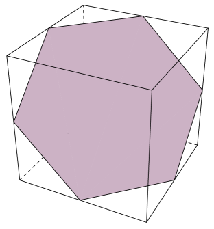
Figure 1. Regular hexagon in ${\mathbb{R}}^{2}$ and in ${\mathbb{R}}^{3}$.

The relation between $(x_{1},x_{2})\in\Omega_{H}$ and ${\mathbf{t}}\in\Omega$ is given by

(2.1) $$t_{1}=-\frac{x_{2}}{2}+\frac{\sqrt{3}x_{1}}{2},\quad t_{2}=x_{2},\quad t_{3}=-\frac{x_{2}}{2}-\frac{\sqrt{3}x_{1}}{2}.$$

For convenience, we adopt the convention of using bold letters, such as ${\mathbf{t}}$, to denote points in the space

$${\mathbb{R}}_{H}^{3}:=\{{\mathbf{t}}=(t_{1},t_{2},t_{3})\in{\mathbb{R}}^{3}:t_{1}+t_{2}+t_{3}=0\}.$$

In other words, bold letters such as ${\mathbf{t}}$ stand for homogeneous coordinates. If we treat $x\in{\mathbb{R}}^{2}$ and ${\mathbf{t}}\in{\mathbb{R}}_{H}^{3}$ as column vectors, then it follows from (2.1) that

(2.2) $$x=\tfrac{1}{3}H(t_{1}-t_{3},t_{2}-t_{3})^{\mathsf{tr}}=\tfrac{1}{3}H(2t_{1}+t_{2},t_{1}+2t_{2})^{\mathsf{tr}}$$

upon using the fact that $t_{1}+t_{2}+t_{3}=0$. Computing the Jacobian of the change of variables shows that $dx=\frac{2\sqrt{3}}{3}dt_{1}dt_{2}$.

A function $f$ is called periodic with respect to the hexagonal lattice, if

$$f(x)=f(x+Hk),\qquad k\in{\mathbb{Z}}^{2}.$$

We call such a function $H$-periodic. In homogeneous coordinates, $x\equiv y\pmod{H}$ becomes, as easily seen using (2.2), ${\mathbf{t}}\equiv{\mathbf{s}}\mod 3$, where we define

$${\mathbf{t}}\equiv{\mathbf{s}}\mod 3\quad\Longleftrightarrow\quad t_{1}-s_{1}\equiv t_{2}-s_{2}\equiv t_{3}-s_{3}\mod 3.$$

Thus, a function $f({\mathbf{t}})$ is $H$-periodic if $f({\mathbf{t}})=f({\mathbf{t}}+{\mathbf{j}})$ whenever ${\mathbf{j}}\equiv 0\mod 3$. If $f$ is $H$-periodic, then it can be verified directly that

(2.3) $$\int_{\Omega}f({\mathbf{t}}+{\mathbf{s}})d{\mathbf{t}}=\int_{\Omega}f({\mathbf{t}})d{\mathbf{t}},\qquad{\mathbf{s}}\in{\mathbb{R}}_{H}^{3}.$$

We define the inner product on the hexagonal domain by

$$\langle f,g\rangle_{H}:=\frac{1}{|\Omega_{H}|}\int_{\Omega_{H}}f(x_{1},x_{2})\overline{g(x_{1},x_{2})}dx_{1}dx_{2}=\frac{1}{|\Omega|}\int_{\Omega}f({\mathbf{t}})\overline{g({\mathbf{t}})}d{\mathbf{t}},$$

where $|\Omega|$ denote the area of $\Omega$. Furthermore, let ${\mathbb{Z}}_{H}^{3}:={\mathbb{Z}}^{3}\cap{\mathbb{R}}_{H}^{3}$. We define

$$\phi_{\mathbf{j}}({\mathbf{t}}):=\mathrm{e}^{\frac{2\pi i}{3}{\mathbf{j}}\cdot{\mathbf{t}}},\qquad{\mathbf{j}}\in{\mathbb{Z}}_{H}^{3},\quad{\mathbf{t}}\in{\mathbb{R}}_{H}^{3}.$$

These exponential functions are orthogonal with respect to ${\langle}f,g{\rangle}_{H}$.

Theorem 2.1.

[6]. For ${\mathbf{k}},{\mathbf{j}}\in{\mathbb{Z}}_{H}^{3}$, ${\langle}\phi_{\mathbf{k}},\phi_{\mathbf{j}}{\rangle}=\delta_{{\mathbf{k}},{\mathbf{j}}}$. Moreover, the set $\{\phi_{\mathbf{j}}:{\mathbf{j}}\in{\mathbb{Z}}_{H}^{3}\}$ is an orthonormal basis of $L^{2}(\Omega)$.

It is easy to see that $\phi_{\mathbf{j}}$ are $H$-periodic functions. We consider a special collection of them indexed by ${\mathbf{j}}$ inside a hexagon. Define

$${\mathbb{H}}_{n}:=\{{\mathbf{j}}\in{\mathbb{Z}}_{H}^{3}:-n\leq j_{1},j_{2},j_{3}\leq n\}\quad\hbox{and}\quad{\mathbb{J}}_{n}:={\mathbb{H}}_{n}\setminus{\mathbb{H}}_{n-1}.$$

Notice that ${\mathbf{j}}\in{\mathbb{H}}_{n}$ satisfies $j_{1}+j_{2}+j_{3}=0$, so that ${\mathbb{H}}_{n}$ contains all integer points inside the hexagon $n\,\overline{\Omega}$, whereas ${\mathbb{J}}_{n}$ contains exactly those integer points in ${\mathbb{Z}}_{H}^{3}$ that are on the boundary of $n\,\Omega$, or $n$-th hexagonal line. We then define

(2.4) $${\mathcal{H}}_{n}:=\operatorname{span}\left\{\phi_{\mathbf{j}}:{\mathbf{j}}\in{\mathbb{H}}_{n}\right\}.$$

It follows that $\dim{\mathcal{H}}_{n}=3n^{2}+3n+1$. As we shall see below, the class ${\mathcal{H}}_{n}$ shares many properties of the class of trigonometric polynomials of one variable. As a result, we shall call functions in ${\mathcal{H}}_{n}$ trigonometric polynomials over $\Omega$. We will study the best approximation by trigonometric polynomials in ${\mathcal{H}}_{n}$ in Section 4.

By Theorem 2.1, the standard Hilbert space theory shows that an $H$-periodic function $f\in L^{2}(\Omega)$ can be expanded into a Fourier series

(2.5) $$f=\sum_{{\mathbf{j}}\in{\mathbb{Z}}_{H}^{3}}\widehat{f}_{\mathbf{j}}\phi_{\mathbf{j}}\quad\hbox{in $L^{2}(\Omega)$},\quad\hbox{where}\quad\widehat{f}_{\mathbf{j}}:=\frac{1}{|\Omega|}\int_{\Omega}f({\mathbf{s}})e^{-\frac{2\pi i{\mathbf{s}}}{3}}d{\mathbf{s}}.$$

We consider the $n$-th hexagonal Fourier partial sum defined by

(2.6) $$S_{n}f(x):=\sum_{{\mathbf{j}}\in{\mathbb{H}}_{n}}\widehat{f}_{\mathbf{j}}\phi_{\mathbf{j}}({\mathbf{t}})=\frac{1}{|\Omega|}\int_{\Omega}f({\mathbf{t}}-{\mathbf{s}})D_{n}({\mathbf{s}})d{\mathbf{s}},$$

where the second equal sign follows from (2.3) with the kernel $D_{n}$ defined by

$$D_{n}({\mathbf{t}}):=\sum_{{\mathbf{j}}\in{\mathbb{H}}_{n}}\phi_{\mathbf{j}}({\mathbf{t}}).$$

The kernel is an analogue of the Dirichlet kernel for the ordinary Fourier series. It enjoys a compact formula given by [13] (see also [10]) that

(2.7) $$D_{n}({\mathbf{t}})=\Theta_{n}({\mathbf{t}})-\Theta_{n-1}({\mathbf{t}}),$$

where

(2.8) $$\Theta_{n}({\mathbf{t}})=\frac{\sin\frac{(n+1)(t_{1}-t_{2})\pi}{3}\sin\frac{(n+1)(t_{2}-t_{3})\pi}{3}\sin\frac{(n+1)(t_{3}-t_{1})\pi}{3}}{\sin\frac{(t_{1}-t_{2})\pi}{3}\sin\frac{(t_{2}-t_{3})\pi}{3}\sin\frac{(t_{3}-t_{1})\pi}{3}}.$$

This last formula is our starting point for studying summability of Fourier series in the following section.

We will also need to use the Poisson summation formula associated with the hexagonal lattice. This formula takes the form (see, for example, [1, 7, 10])

(2.9) $$\sum_{k\in{\mathbb{Z}}^{2}}f(x+Hk)=\frac{1}{\det(H)}\sum_{j\in{\mathbb{Z}}^{2}}\widehat{f}(H^{-{\mathsf{tr}}}k)e^{2\pi ik^{\mathsf{tr}}H^{-1}{\mathbf{x}}},$$

where for $f\in L^{1}({\mathbb{R}}^{2})$ the Fourier transform $\widehat{f}$ and its inverse are defined by

$$\widehat{f}(\xi)=\int_{{\mathbb{R}}^{2}}f(x)\mathrm{e}^{-2\pi\xi\cdot x}dx\quad\hbox{and}\quad f(x)=\int_{{\mathbb{R}}^{2}}\widehat{f}(\xi)\mathrm{e}^{2\pi\xi\cdot x}dx,$$

and the formula holds under the usual assumption on the convergence of the series in both sides. Define Fourier transform in homogeneous coordinates by $\widehat{f}({\mathbf{t}}):=\widehat{f}(H^{-{\mathsf{tr}}}t)$ with $t=(t_{1},t_{2})$ as a column vector. Using (2.2), it is easy to see that $\widehat{f}$ and its inverse become, in homogeneous coordinates,

(2.10) $$\widehat{f}({\mathbf{s}})=\int_{{\mathbb{R}}_{H}^{3}}f({\mathbf{t}})\mathrm{e}^{-\frac{2\pi i}{3}{\mathbf{s}}\cdot{\mathbf{t}}}d{\mathbf{t}}\qquad\hbox{and}\qquad f({\mathbf{t}})=\int_{{\mathbb{R}}_{H}^{3}}\widehat{f}({\mathbf{s}})\mathrm{e}^{\frac{2\pi i}{3}{\mathbf{s}}\cdot{\mathbf{t}}}d{\mathbf{s}}.$$

Next we reformulate Poisson summation formula in homogenous coordinates. The left hand side of (2.9) is an $H$-periodic function over hexagonal lattice, which becomes the summation of $f({\mathbf{t}}+3{\mathbf{j}})$ over all ${\mathbf{j}}\in{\mathbb{Z}}_{H}^{3}$ as $x\equiv y\mod H$ becomes ${\mathbf{t}}\equiv{\mathbf{s}}\mod 3$. For the right hand side, using the fact that $(k_{1},k_{2})H^{-1}x=\frac{1}{3}(k_{1},k_{2})(t_{1}-t_{3},t_{2}-t_{3})^{\mathsf{tr}}=\frac{1}{3}{\mathbf{k}}\cdot{\mathbf{t}}$ by (2.2), we obtain

$$\widehat{f}(H^{-{\mathsf{tr}}}k)=\int_{{\mathbb{R}}^{2}}f(x)\mathrm{e}^{-2\pi k^{\mathsf{tr}}H^{-1}x}dx=\frac{2\sqrt{3}}{3}\int_{{\mathbb{R}}_{H}^{3}}f({\mathbf{t}})\mathrm{e}^{-2\pi{\mathbf{k}}\cdot{\mathbf{t}}}d{\mathbf{t}}=\frac{2\sqrt{3}}{3}\widehat{f}({\mathbf{k}}).$$

Consequently, we conclude that the Poisson summation formula in (2.9) becomes, in homogeneous coordinates,

(2.11) $$\sum_{{\mathbf{k}}\in{\mathbb{Z}}_{H}^{3}}f({\mathbf{t}}+3{\mathbf{k}})=\frac{1}{3}\sum_{{\mathbf{j}}\in{\mathbb{Z}}_{H}^{3}}\widehat{f}({\mathbf{j}})\mathrm{e}^{\frac{2\pi i}{3}{\mathbf{j}}\cdot{\mathbf{t}}}.$$

Throughout of this paper we will reserve the letter $c$ for a generic constant, whose value may change from line to line. By $A\sim B$ we mean that there are two constants $c$ and $c^{\prime}$ such that $cA\leq B\leq c^{\prime}A$.

3. Summability of Fourier series on Hexagon

We consider hexagonal summability of Fourier series (2.5); that is, we write the Fourier series (2.5) as blocks whose indices are grouped according to ${\mathbb{J}}_{n}$:

$$f({\mathbf{t}})=\sum_{n=0}^{\infty}\sum_{{\mathbf{j}}\in{\mathbb{J}}_{n}}\widehat{f}_{\mathbf{j}}\phi_{{\mathbf{j}}}({\mathbf{t}}).$$

From now on we call such a series hexagonal Fourier series. Its $n$-th partial sum is exactly $S_{n}f$ given in (2.6).

3.1. Abel summability

We consider Poisson integral $P_{r}f(t)$ of the hexagon Fourier series, which is defined by

$$P_{r}f({\mathbf{t}}):=\sum_{n=0}^{\infty}\sum_{{\mathbf{j}}\in{\mathbb{J}}_{n}}\widehat{f}_{\mathbf{j}}\phi_{\mathbf{j}}({\mathbf{t}})r^{n}=\frac{1}{\Omega}\int_{|\Omega|}P(r;{\mathbf{t}}-{\mathbf{s}})f({\mathbf{s}})d{\mathbf{s}},$$

where $P(r;{\mathbf{t}})$ denotes the Poisson kernel

$$P(r;{\mathbf{t}}):=\sum_{n=0}^{\infty}\sum_{{\mathbf{j}}\in{\mathbb{J}}_{n}}\phi_{\mathbf{j}}({\mathbf{t}})r^{n},\qquad 0\leq r<1.$$

Just as in the classical Fourier series, the kernel is nonnegative and enjoys a closed expression.

Proposition 3.1.

(1) The Poisson kernel $P(r;{\mathbf{t}})$ is nonnegative for all ${\mathbf{t}}\in\Omega$ and

$$\frac{1}{|\Omega}\int_{\Omega}P(r;{\mathbf{t}})d{\mathbf{t}}=1.$$

(2) Let $q(r,t)=1-2r\cos t+r^{2}$. Then

$$P(r;{\mathbf{t}})= \frac{(1-r)^{3}(1-r^{3})}{q\left(r,\frac{2\pi(t_{1}-t_{2})}{3}\right)q\left(r,\frac{2\pi(t_{2}-t_{3})}{3}\right)q\left(r,\frac{2\pi(t_{3}-t_{1})}{3}\right)}$$

$$+\frac{r(1-r)^{2}}{q\left(r,\frac{2\pi(t_{1}-t_{2})}{3}\right)q\left(r,\frac{2\pi(t_{2}-t_{3})}{3}\right)}+\frac{r(1-r)^{2}}{q\left(r,\frac{2\pi(t_{2}-t_{3})}{3}\right)q\left(r,\frac{2\pi(t_{3}-t_{1})}{3}\right)}$$

$$+\frac{r(1-r)^{2}}{q\left(r,\frac{2\pi(t_{3}-t_{1})}{3}\right)q\left(r,\frac{2\pi(t_{1}-t_{2})}{3}\right)}.$$

Proof.

The fact that the integral of $P(r;{\mathbf{t}})$ is 1 follows from the definition and the orthogonality of $\phi_{\mathbf{j}}(t)$, whereas that $P(r;{\mathbf{t}})\geq 0$ is an immediate consequence of the compact formula in the part (2).

To prove the part (2), we start from the compact formula of $D_{n}({\mathbf{t}})$, from which follows readily that

$$P(r;{\mathbf{t}})=(1-r)\sum_{n=0}^{\infty}D_{n}({\mathbf{t}})r^{n}=(1-r)^{2}\sum_{n=0}^{\infty}\Theta_{n}({\mathbf{t}})r^{n}.$$

If $t_{1}+t_{2}+t_{3}=0$ then it is easy to verify that

(3.1) $$\begin{split}&\sin 2t_{1}+\sin 2t_{2}+\sin 2t_{3}=-4\sin t_{1}\sin t_{2}\sin t_{3},\\ &\cos 2t_{1}+\cos 2t_{2}+\cos 2t_{3}=4\cos t_{1}\cos t_{2}\cos t_{3}-1.\end{split}$$

Using the first equation in (3.1) and the fact that

$$\sum_{n=0}^{\infty}\sin(n+1)s=\frac{\sin s}{1-2r\cos s+r^{2}},$$

we conclude then

$$\sum_{n=0}^{\infty}\Theta_{n}({\mathbf{t}})r^{n}= \frac{1}{4\sin\frac{\pi(t_{1}-t_{2})}{3}\sin\frac{\pi(t_{2}-t_{3})}{3}\sin\frac{\pi(t_{3}-t_{1})}{3}}$$

$$\times\left[\frac{\sin\frac{2\pi(t_{1}-t_{2})}{3}}{q\left(r,\frac{2\pi(t_{1}-t_{2})}{3}\right)}+\frac{\sin\frac{2\pi(t_{2}-t_{3})}{3}}{q\left(r,\frac{2\pi(t_{2}-t_{3})}{3}\right)}+\frac{\sin\frac{2\pi(t_{3}-t_{1})}{3}}{q\left(r,\frac{2\pi(t_{3}-t_{1})}{3}\right)}\right].$$

Putting the three terms together and simplify the numerator, we conclude, after a tedious computation, that

$$\sum_{n=0}^{\infty}\Theta_{n}({\mathbf{t}})r^{n}=\frac{1+2r+2r^{3}+r^{4}-2r^{2}\left[\cos\frac{2\pi(t_{1}-t_{2})}{3}+\cos\frac{2\pi(t_{1}-t_{3})}{3}+\cos\frac{2\pi(t_{2}-t_{3})}{3}\right]}{q\left(r,\frac{2\pi(t_{1}-t_{2})}{3}\right)q\left(r,\frac{2\pi(t_{2}-t_{3})}{3}\right)q\left(r,\frac{2\pi(t_{3}-t_{1})}{3}\right)}.$$

The numerator of the right hand side can be written as

$$(1-r)(1-r^{3})+r\left[\left(r,\tfrac{2\pi(t_{1}-t_{2})}{3}\right)+q\left(r,\tfrac{2\pi(t_{2}-t_{3})}{3}\right)+q\left(r,\tfrac{2\pi(t_{3}-t_{1})}{3}\right)\right],$$

from which the stated compact formula follows. ∎

Next we consider the convergence of $P_{r}f$ as $r\to 1-$. For the classical Fourier series, if $P_{r}f$ converges to $f$ as $r\to 1-$ then the series is called Abel summable.

Theorem 3.2.

If $f$ is an $H$-periodic function, bounded on $\overline{\Omega}$ and continuous at ${\mathbf{t}}\in\Omega^{\circ}$, then $P_{r}f({\mathbf{t}})$ converges to $f({\mathbf{t}})$ as $r\mapsto 1-$. Furthermore, if $f$ is continuous on $\overline{\Omega}$, then $P_{r}f$ converges uniformly on $\Omega$ as $r\mapsto 1-$.

Proof.

Since $f$ is continuous at ${\mathbf{t}}\in\Omega^{\circ}$. For any ${\varepsilon}>0$, choose ${\delta}>0$ such that

$$|f({\mathbf{t}}-{\mathbf{s}})-f({\mathbf{t}})|<{\varepsilon}\qquad\hbox{whenever ${\mathbf{s}}\in\Omega_{\delta}:=\{{\mathbf{s}}\in\Omega:|s_{i}|\leq{\delta},\,1\leq i\leq 3\}$}.$$

Since $P(r;{\mathbf{s}})$ has a unit integral, it follows that

$$|P_{r}f({\mathbf{t}})-f({\mathbf{t}})| \leq{\varepsilon}\int_{\Omega_{\delta}}P(r;{\mathbf{s}})d{\mathbf{s}}+2\int_{\Omega\setminus\Omega_{\delta}}|f({\mathbf{t}}-{\mathbf{s}})-f({\mathbf{t}})|P(r;{\mathbf{s}})d{\mathbf{s}}$$

$$\leq{\varepsilon}+2\|f\|_{\infty}\int_{\Omega\setminus\Omega_{\delta}}P(r;{\mathbf{s}})d{\mathbf{s}}.$$

Thus, it suffices to show that the last integral goes to 0 as $r\mapsto 1+$. Since $q(r,t)=(1-r)^{2}+2r\sin^{2}\frac{t}{2}\geq(1-r)^{2}$, the closed formula of the Poisson kernel shows that $P_{r}({\mathbf{t}})$ is bounded by

$$P(r;{\mathbf{t}}) \leq\frac{2(1-r)^{2}}{q\left(r,\frac{2\pi(t_{1}-t_{2})}{3}\right)q\left(r,\frac{2\pi(t_{2}-t_{3})}{3}\right)}+\frac{2(1-r)^{2}}{q\left(r,\frac{2\pi(t_{2}-t_{3})}{3}\right)q\left(r,\frac{2\pi(t_{3}-t_{1})}{3}\right)}$$

$$+\frac{2(1-r)^{2}}{q\left(r,\frac{2\pi(t_{3}-t_{1})}{3}\right)q\left(r,\frac{2\pi(t_{1}-t_{2})}{3}\right)}.$$

Clearly we only need to consider one of the three terms in the right hand side, say the second one, so that the essential task is reduced to show that, as $q(r,t)$ is even in $t$,

(3.2) $$\lim_{r\to 1+}\int_{\Omega\setminus\Omega_{\delta}}\frac{(1-r)^{2}}{q\left(r,\frac{2\pi(t_{1}-t_{3})}{3}\right)q\left(r,\frac{2\pi(t_{2}-t_{3})}{3}\right)}d{\mathbf{s}}=0.$$

Setting $P(r;t):=\frac{1-r^{2}}{q(r,t)}$ for $-\pi\leq t\leq\pi$. Then $P(r;t)$ is the Poisson kernel for the classical Fourier series. It is known [16] that

(3.3) $$\int_{-\pi}^{\pi}P(r;t)dt=1\qquad\hbox{and}\qquad 0\leq P(r;t)\leq c\frac{1-r}{t^{2}},$$

where $c$ is a constant independent of $r$ and $t$. Evidently, the kernel in the left hand side of (3.2) can be written as

$$\frac{(1-r)^{2}}{q\left(r,\frac{2\pi(t_{1}-t_{3})}{3}\right)q\left(r,\frac{2\pi(t_{2}-t_{3})}{3}\right)}=\frac{1}{(1+r)^{2}}P\left(r;\tfrac{2\pi(t_{1}-t_{3})}{3}\right)P\left(r,\tfrac{2\pi(t_{2}-t_{3})}{3}\right).$$

Recall that $t_{1}+t_{2}+t_{3}=0$ for ${\mathbf{t}}=(t_{1},t_{2},t_{3})\in\Omega$. It is easy to see that ${\mathbf{t}}\in\overline{\Omega}$ means that $-1\leq t_{1},t_{2},t_{1}-t_{2}\leq 1$. Let

(3.4) $$s_{1}:=\frac{t_{1}-t_{3}}{3}=\frac{2t_{1}+t_{2}}{3},\qquad s_{2}:=\frac{t_{2}-t_{3}}{3}=\frac{t_{1}+2t_{2}}{3}.$$

A simple geometric consideration shows that the image of the domain $\Omega_{\delta}$ under the affine mapping $(t_{1},t_{2})\mapsto(s_{1},s_{2})$ in (3.4) contains the square $[-{\delta}/6,{\delta}/6]^{2}$. Consequently, the image of $\overline{\Omega}\setminus\Omega_{\delta}$ is a subset of $[-1,1]^{2}\setminus[-{\delta}/6,{\delta}/6]^{2}$. Hence, changing variables $(t_{1},t_{2})\mapsto(s_{1},s_{2})$, we obtain by (3.3) that

$$\int_{\Omega\setminus\Omega_{\delta}}\frac{(1-r)^{2}}{q\left(r,\frac{2\pi(t_{1}-t_{3})}{3}\right)q\left(r,\frac{2\pi(t_{2}-t_{3})}{3}\right)}d{\mathbf{t}}$$

$$\qquad\qquad\leq\frac{3}{(1+r)^{2}}\int_{[-1,1]^{2}\setminus[-{\delta}/6,{\delta}/6]^{2}}{P\left(r,2\pi s_{1}\right)P\left(r,2\pi s_{2}\right)}d{\mathbf{s}}$$

$$\qquad\qquad\leq 3\int_{1\geq|s|\geq\delta/6}P(r,2\pi s)ds\leq c\frac{1-r}{{\delta}},$$

which converges to zero when $r\to 1-$. This proves (3.2) and the convergence of $P_{r}f({\mathbf{t}})$ to $f({\mathbf{t}})$. Clearly it also proves the uniform convergence of $P_{r}f$ to $f\in C(\overline{\Omega})$. ∎

3.2. Cesàro summability

Let us denote by $S_{n}^{\delta}f$ and $K_{n}^{\delta}$ the Cesàro $(C,{\delta})$ means of the hexagonal Fourier series and its kernel, respectively. Then

$$S_{n}^{\delta}f({\mathbf{t}}):=\int_{\Omega}f({\mathbf{s}})K_{n}^{({\delta})}(tb-{\mathbf{s}})d{\mathbf{s}},$$

where

$$K_{n}^{({\delta})}({\mathbf{t}}):=\frac{1}{A_{n}^{\delta}}\sum_{k=0}^{n}A_{n-k}^{\delta}\sum_{{\mathbf{j}}\in{\mathbb{J}}_{n}}\phi_{\mathbf{j}}({\mathbf{t}}),\qquad A_{n}^{\delta}=\binom{n+{\delta}}{{\delta}}.$$

It is evident that the case ${\delta}=0$ corresponds to $S_{n}f$ and $D_{n}({\mathbf{t}})$, respectively. By (2.7) and (2.8), the $(C,1)$ kernel is given by

$$K_{n}^{(1)}({\mathbf{t}})=\frac{1}{n}\Theta_{n}({\mathbf{t}})=\frac{1}{n}\frac{\sin\frac{(n+1)(t_{1}-t_{2})\pi}{3}\sin\frac{(n+1)(t_{2}-t_{3})\pi}{3}\sin\frac{(n+1)(t_{3}-t_{1})\pi}{3}}{\sin\frac{(t_{1}-t_{2})\pi}{3}\sin\frac{(t_{2}-t_{3})\pi}{3}\sin\frac{(t_{3}-t_{1})\pi}{3}}.$$

For the classical Fourier series in one variable, the $(C,1)$ kernel is the well-known Fejèr kernel, which is given by

$$\frac{1}{n+1}\sum_{k=0}^{n}D_{k}(t)=\frac{1}{n+1}\left(\frac{\sin\frac{(n+1)t}{2}}{\sin\frac{t}{2}}\right)^{2}$$

and is nonnegative in particular. For the hexagonal Fourier series, it turns out that $K_{n}^{(2)}$ is nonnegative.

Lemma 3.3.

For $n\geq 0$,

$$\binom{n+2}{2}K_{n}^{(2)}({\mathbf{t}})=\frac{1}{16}\frac{A_{n}({\mathbf{t}})^{2}+B_{n}({\mathbf{t}})^{2}}{\left(\sin\frac{(t_{1}-t_{2})\pi}{3}\right)^{2}\left(\sin\frac{(t_{2}-t_{3})\pi}{3}\right)^{2}\left(\sin\frac{(t_{3}-t_{1})\pi}{3}\right)^{2}},$$

where

$$A_{n}({\mathbf{t}}) \,:=\cos\tfrac{nt_{1}\pi}{3}\sin\tfrac{(n+2)(t_{2}-t_{3})\pi}{3}+\cos\tfrac{nt_{2}\pi}{3}\sin\tfrac{(n+2)(t_{3}-t_{1})\pi}{3}+\cos\tfrac{nt_{3}\pi}{3}\sin\tfrac{(n+2)(t_{1}-t_{2})\pi}{3},$$

$$B_{n}({\mathbf{t}}) \,:=\sin\tfrac{nt_{1}\pi}{3}\sin\tfrac{(n+2)(t_{2}-t_{3})\pi}{3}+\sin\tfrac{nt_{2}\pi}{3}\sin\tfrac{(n+2)(t_{3}-t_{1})\pi}{3}+\sin\tfrac{nt_{3}\pi}{3}\sin\tfrac{(n+2)(t_{1}-t_{2})\pi}{3}.$$

Proof.

Using (3.1) and the elementary formula

$$\sum_{k=0}^{n}\sin[2(k+1)s]=\frac{\sin[(n+1)s]\sin[(n+2)s]}{\sin s},$$

we obtain

$$\sum_{k=0}^{n}\Theta_{k}({\mathbf{t}})=\frac{-4E_{n}({\mathbf{t}})}{\left(\sin\frac{(t_{1}-t_{2})\pi}{3}\right)^{2}\left(\sin\frac{(t_{2}-t_{3})\pi}{3}\right)^{2}\left(\sin\frac{(t_{3}-t_{1})\pi}{3}\right)^{2}}.$$

where

$$E_{n}({\mathbf{t}}):= \sin\tfrac{(n+1)(t_{1}-t_{2})\pi}{3}\sin\tfrac{(n+2)(t_{1}-t_{2})\pi}{3}\sin\tfrac{(t_{2}-t_{3})\pi}{3}\sin\tfrac{(t_{3}-t_{1})\pi}{3}$$

$$+ \sin\tfrac{(n+1)(t_{2}-t_{3})\pi}{3}\sin\tfrac{(n+2)(t_{2}-t_{3})\pi}{3}\sin\tfrac{(t_{1}-t_{2})\pi}{3}\sin\tfrac{(t_{3}-t_{1})\pi}{3}$$

$$+ \sin\tfrac{(n+1)(t_{3}-t_{1})\pi}{3}\sin\tfrac{(n+2)(t_{3}-t_{1})\pi}{3}\sin\tfrac{(t_{1}-t_{2})\pi}{3}\sin\tfrac{(t_{2}-t_{3})\pi}{3}.$$

From here, the difficulty lies in identifying that the numerator is a sum of squares. Once the form is recognized, the verification that $-4E_{n}({\mathbf{t}})=\frac{1}{16}((A_{n}({\mathbf{t}})^{2}+B_{n}({\mathbf{t}})^{2})$ is a straightforward, though tedious, exercise. ∎

An immediate consequence of the above lemma is the following:

Theorem 3.4.

The $(C,2)$ means of the Fourier expansion with respect to the hexagon domain is a positive linear opreator.

As a comparison, let us mention that for the usual Fourier series on the tours, if the partial sums are defined with respect to $\ell^{\infty}$ ball, that is, if the Dirichlet kernel is defined as

$$D_{n}({\theta}_{1},{\theta}_{2})=\sum_{-n\leq k_{1},k_{2}\leq n}e^{i(k_{1}{\theta}_{1}+k_{2}{\theta}_{2})},\quad({\theta}_{1},{\theta}_{2})\in[-\pi,\pi]^{2},$$

then it is proved in [2] that the corresponding $(C,3)$ means are nonnegative and $\delta=3$ is sharp. In fact, the results in [2] are established for the partial sums defined with respect to the $\ell^{1}$ ball for $d$-dimensional torus. For $d=2$, it is easy to see that the result on $\ell^{1}$ ball implies the result on $\ell^{\infty}$ ball.

If the $(C,{\delta})$ means converge to $f$, then so is $(C,{\delta}^{\prime})$ means for ${\delta}^{\prime}>{\delta}$. The positivity of the kernel shows immediately that $(C,2)$ means of the hexagonal Fourier series converges. It turns out that the $(C,1)$ means is enough.

Theorem 3.5.

If $f\in C(\overline{\Omega})$, then the $(C,1)$ means $S_{n}^{(1)}f$ converge uniformly to $f$ in $\overline{\Omega}$.

Proof.

A standard argument shows that it suffices to prove that $S_{n}^{(1)}$ is a bounded operator, which amounts to show that

$$I_{n}:=\int_{\Omega}\left|\Theta_{n}({\mathbf{t}})\right|d{\mathbf{t}}\leq c\,n$$

Since $\Theta_{n}({\mathbf{t}})$ is a symmetric function in $t_{1},t_{2},t_{3}$, we only need to consider the integral over the triangle

$$\Delta:=\{{\mathbf{t}}\in{\mathbb{R}}_{\mathbb{H}}:0\leq t_{1},t_{2},-t_{3}\leq 1\}=\{(t_{1},t_{2}):t_{1}\geq 0,t_{2}\geq 0,t_{1}+t_{2}\leq 1\},$$

which is one of the six triangle in $\Omega$ (see Figure 1). Let $s_{1},s_{2}$ be defined as in (3.4) and let $\Delta^{*}$ denote the image of $\Delta$ in $(s_{1},s_{2})$ plane. Then

$$\widetilde{\Delta}=\{(s_{1},s_{2}):0\leq s_{1}\leq 2s_{2},0\leq s_{2}\leq 2s_{1},s_{1}+s_{2}\leq 1\}$$

and it follows, as the Jacobian of the change of variables is equal to 3, that

$$I_{n}=3\int_{\widetilde{\Delta}}\left|\frac{\sin((n+1)\pi s_{1})\sin((n+1)\pi s_{2})\sin((n+1)\pi(s_{1}-s_{2}))}{\sin(\pi s_{1})\sin(\pi s_{2})\sin(\pi(s_{1}+s_{2}))}\right|ds_{1}ds_{2}.$$

Since the integrant in the right hand side is clearly a symmetric function of $(s_{1},s_{2})$, it is equal to twice of the integral over half of the $\widetilde{\Delta}$, say over

$$\widetilde{\Delta}^{*}=\{(s_{1},s_{2})\in\widetilde{\Delta}:s_{1}\leq s_{2}\}=\{(s_{1},s_{2}):s_{1}\leq s_{2}\leq 2s_{1},s_{1}+s_{2}\leq 1\}.$$

Making another change of variables $s_{1}=(u_{1}-u_{2})/2$ and $s_{2}=(u_{1}+u_{2})/2$, the domain $\widetilde{\Delta}^{*}$ becomes $\Gamma:=\{(u_{1},u_{2}):0\leq u_{2}\leq u_{1}/3,0\leq u_{1}\leq 1\}$ and we conclude that

$$I_{n}=3\int_{\Gamma}\left|\frac{\sin\frac{(n+1)(u_{1}+u_{2})\pi}{2}\sin\frac{(n+1)(u_{1}-u_{2})\pi}{2}\sin\frac{(n+1)u_{2}\pi}{2}}{\sin\frac{(u_{1}+u_{2})\pi}{2}\sin\frac{(u_{1}-u_{2})\pi}{2}\sin\frac{u_{2}\pi}{2}}\right|du_{1}du_{2}:=3\int_{\Gamma}|\Theta_{n}^{*}(u)|du$$

To estimate the last integral, we partition $\Gamma$ as $\Gamma=\Gamma_{1}\cup\Gamma_{2}\cup\Gamma_{3}$ and consider the three cases separately.

Case 1. $\Gamma_{1}=\{u\in\Gamma:u_{1}\leq 3/n\}$. Using the fact that $|\sin nt/\sin t|\leq n$, we obtain

$$\int_{\Gamma_{1}}|\Theta_{n}^{*}(u)|du\leq(n+1)^{3}\int_{\Gamma_{1}}du_{1}du_{2}=(n+1)^{3}\frac{3n^{2}}{2}\leq c\,n.$$

Case 2. $\Gamma_{2}=\{u\in\Gamma:3/n\leq u_{1},\,u_{2}\leq 1/n\}$. In this region we have $u_{1}-u_{2}\geq 2u_{1}/3$ and $u_{1}+u_{2}\geq u_{1}$. Hence, upon using $\sin u\geq(2/\pi)u$, we obtain

$$\int_{3/n}^{1}\left|\frac{\sin\frac{(n+1)(u_{1}+u_{2})\pi}{2}\sin\frac{(n+1)(u_{1}-u_{2})\pi}{2}}{\sin\frac{(u_{1}+u_{2})\pi}{2}\sin\frac{(u_{1}-u_{2})\pi}{2}}\right|du_{1}\leq\int_{3/n}^{1}\frac{1}{u_{1}^{2}}du_{1}\leq c\,n.$$

Consequently, it follows that

$$\int_{\Gamma_{2}}|\Theta_{n}^{*}(u)|du=\int_{0}^{1/n}\int_{3/n}^{1}|\Theta_{n}^{*}(u)|du\leq c\,n\int_{0}^{1/n}\left|\frac{\sin\frac{(n+1)u_{2}\pi}{2}}{\sin\frac{u_{2}\pi}{2}}\right|\leq c\,n$$

upon using $|\sin nu/\sin u|\leq n$ again.

Case 3. $\Gamma_{3}=\{u\in\Gamma:3/n\leq u_{,}\,u_{2}\geq 1/n\}$. In this region we have $u_{1}\geq 3u_{2}$, which implies that $u_{1}-u_{2}\geq(2/3)u_{1}$ and $u_{1}+u_{2}\geq u_{1}$. Thus, using $\sin u\geq(2/\pi)u$ again, we obtain

$$\int_{3u_{2}}^{1}\left|\frac{\sin\frac{(n+1)(u_{1}+u_{2})\pi}{2}\sin\frac{(n+1)(u_{1}-u_{2})\pi}{2}}{\sin\frac{(u_{1}+u_{2})\pi}{2}\sin\frac{(u_{1}-u_{2})\pi}{2}}\right|du_{1}\leq c\int_{3u_{2}}^{1}\frac{1}{u_{1}^{2}}du_{1}\leq\frac{c}{u_{2}}.$$

Consequently, using $\sin u_{2}\geq(2/\pi)u_{2}$, we conclude that

$$\int_{\Gamma_{3}}|\Theta_{n}^{*}(u)|du=\int_{0}^{1/n}\int_{3/n}^{1}|\Theta_{n}^{*}(u)|du\leq c\int_{1/n}^{1/3}\frac{1}{u_{2}^{2}}du_{2}\leq c\,n.$$

Putting these estimates together completes the proof. ∎

This theorem shows that $(C,{\delta})$ summability of the hexagonal Fourier series behaviors just like that of classical Fourier series. In particular, we naturally conjecture that the $(C,\delta)$ means of the hexagonal Fourier series should converge if ${\delta}>0$. This condition is sharp as ${\delta}=0$ corresponds to $S_{n}f$ whose norm is known to be in the order of $(\log n)^{2}$ ([12, 13]).

4. Best Approximation on Hexagon

For $1\leq p\leq\infty$ we define $L^{p}$ space to be the space of Lebesgue integrable $H$-periodic functions on $\Omega$ with the norm

$$\|f\|_{p}:=\left(\int_{\Omega}|f({\mathbf{t}})|^{p}d{\mathbf{t}}\right)^{1/p},\qquad 1\leq p<\infty,$$

and we assume that $L^{p}$ is $C(\overline{\Omega})$ when $p=\infty$, with the uniform norm on $\overline{\Omega}$. For $f\in L^{p}$, we define the error of best approximation to $f$ from ${\mathcal{H}}_{n}$ by

$$E_{n}(f)_{p}:=\inf_{S\in{\mathcal{H}}_{n}}\|f-S\|_{p}.$$

We shall prove the direct and inverse theorems using a modulus of smoothness.

4.1. A simple fact

We start with an observation that $E_{n}(f)$ can be related to the error of best approximation by trigonometric polynomials of two variables on $[-1,1]^{2}$. To see this, let us denote by ${\mathcal{T}}_{n}$ the space of trigonometric polynomials of two variables of degree $n$ in each variable, whose elements are of the form

$$T(u)=\sum_{k_{1}=0}^{n}\sum_{k_{2}=0}^{n}b_{k}\mathrm{e}^{2\pi i(k_{1}u_{1}+k_{2}u_{2})}.$$

Furthermore, if $f\in C([-1,1]^{2})$ and it is $2\pi$ periodic in both variables, then define

$${\mathcal{E}}_{n}(f):=\inf_{T\in{\mathcal{T}}_{n}}\max_{u\in[-1,1]^{2}}|f(u)-T(u)|.$$

Proposition 4.1.

Let $f$ be $H$-periodic and continuous over the regular hexagon $\overline{\Omega}_{H}$. Assume that $f^{*}$ is a continuous extension of $f$ on $[-1,1]^{2}$. Then

$$E_{n}(f)\leq{\mathcal{E}}_{\lfloor\frac{n}{2}\rfloor}(f^{*}).$$

Proof.

We again work with homogeneous coordinates. Using the fact that $t_{1}+t_{2}+t_{3}=0$ and $j_{1}+j_{2}+j_{3}=0$, we can write

$$\phi_{{\mathbf{j}}}({\mathbf{t}})=e^{\frac{2\pi i}{3}{\mathbf{j}}\cdot{\mathbf{t}}}=e^{2\pi i(j_{1}s_{1}+j_{2}s_{2})},\qquad s_{1}=\tfrac{2t_{1}+t_{2}}{3},\quad s_{2}=\tfrac{t_{1}+2t_{2}}{3}.$$

Clearly ${\mathbf{t}}\in\overline{\Omega}$ implies that $(s_{1},s_{2})\in\Omega^{*}:=\{s:-1\leq s_{1},s_{2},s_{1}+s_{2}\leq 1\}$. Furthermore, ${\mathbf{j}}\in{\mathbb{H}}_{n}$ implies that $-n\leq j_{1},j_{2},j_{1}+j_{2}\leq n$. Consequently, we have that

$$S_{n}({\mathbf{t}}):=\sum_{j\in{\mathcal{H}}_{n}}c_{\mathbf{j}}\phi_{\mathbf{j}}({\mathbf{t}})=\sum_{\begin{subarray}{c}-n\leq j_{1},j_{2}\leq n\\ -n\leq j_{1}+j_{2}\leq n\end{subarray}}c_{j_{1},j_{2},-j_{1}-j_{2}}e^{2\pi i(j_{1}s_{1}+j_{2}s_{2})}:=T_{n}(s).$$

Let $g(s)=f({\mathbf{t}})=f(2s_{1}-s_{2},2s_{2}-s_{1},-s_{1}-s_{2})$ and let its continuous extension to $[-1,1]^{2}$ be $g^{*}$. It follows that

$$\|f-S_{n}\|=\max_{s\in\Omega^{*}}|g(s)-T_{n}(s)|\leq\max_{-1\leq s_{1},s_{2}\leq 1}|g^{*}(s)-T_{n}(s)|.$$

Taking minimum over all $S_{n}\in{\mathcal{H}}_{n}$ translates to taking minimal of all $c_{\mathbf{j}}$, consequently we conclude that

$$E_{n}(f) \,\leq\min_{c_{\mathbf{j}}}\max_{-1\leq s_{1},s_{2}\leq 1}\left|g^{*}(s)-\sum_{\begin{subarray}{c}-n\leq j_{1},j_{2}\leq n\\ -n\leq j_{1}+j_{2}\leq n\end{subarray}}c_{\mathbf{j}}\mathrm{e}^{2\pi i(j_{1}s_{1}+j_{2}s_{2})}\right|$$

$$\,\leq\min_{c_{\mathbf{j}}}\max_{-1\leq s_{1},s_{2}\leq 1}\left|g^{*}(s)-\sum_{-\lfloor\frac{n}{2}\rfloor\leq j_{1},j_{2}\leq\lfloor\frac{n}{2}\rfloor}c_{\mathbf{j}}\mathrm{e}^{2\pi i(j_{1}s_{1}+j_{2}s_{2})}\right|={\mathcal{E}}_{\lfloor\frac{n}{2}\rfloor}(g^{*}).$$

If we work with $f$ defined on $\Omega_{H}$, then $g^{*}$ becomes $f^{*}$ in the statement of the proposition. ∎

For smooth functions, this result can be used to derive the convergence order of $E_{n}(f)$. The procedure of the proof, however, is clearly only one direction. Below we prove both direct and inverse theorems using a modulus of smoothness.

4.2. Modulus of smoothness

On the set $\Omega$, we can define a modulus of smoothness by following precisely the definition for periodic functions on the real line. Thus, we define for $r\in{\mathbb{N}}_{0}$,

$$\Delta_{\mathbf{t}}f({\mathbf{x}})=f({\mathbf{x}}+{\mathbf{t}})-f({\mathbf{x}}),\qquad\Delta_{\mathbf{t}}^{r}f({\mathbf{x}})=\Delta_{\mathbf{t}}\Delta_{\mathbf{t}}^{r-1}f({\mathbf{x}}).$$

It is well known that

$$\Delta_{\mathbf{t}}f({\mathbf{x}})=\sum_{k=0}^{r}(-1)^{k}\binom{r}{k}f({\mathbf{x}}+k{\mathbf{t}}).$$

For ${\mathbf{t}}\in{\mathbb{R}}_{\mathbb{H}}$, let $\|{\mathbf{t}}\|:=(t_{1}^{2}+t_{2}^{2})^{1/2}$, the usual Euclidean norm of $(t_{1},t_{2})$. We can also take other norm of $(t_{1},t_{2})$ instead, for example, $\|{\mathbf{t}}\|_{\infty}:=\max\{|t_{1}|,|t_{2}|\}$. Since $t_{1}+t_{2}+t_{3}=0$, we have evidently $\|{\mathbf{t}}\|_{\infty}\leq\max\{|t_{1}|,|t_{2}|,|t_{3}|\}\leq 2\|{\mathbf{t}}\|_{\infty}$. The modulus of smoothness of an $H$-periodic function $f$ is then defined as

$$\omega_{r}(f;h)_{p}:=\sup_{\|{\mathbf{t}}\|\leq h}\|\Delta_{\mathbf{t}}^{r}f\|_{p},\qquad 1\leq p\leq\infty.$$

Proposition 4.2.

The modulus of smoothness satisfies the following properties:

1. For $\lambda>0$, $\omega_{r}(f;\lambda h)_{p}\leq(1+\lambda)^{r}\omega_{r}(f;h)_{p}$.

2. Let $\partial_{i}$ denote the partial derivative with respect to $t_{i}$ and $\partial^{k}=\partial_{1}^{k_{1}}\partial_{2}^{k_{2}}\partial_{3}^{k_{2}}$ for $k=(k_{1},k_{2},k_{3})$. Then

   $$\omega_{r}(f;h)_{p}\leq h^{r}\sum_{k_{1}+k_{2}+k_{3}=r}\frac{r!}{k_{1}!k_{2}!k_{3}!}\|\partial^{k}f\|_{p}.$$

Proof.

The proof of (1) follows exactly as in the proof of one variable. For part (2), it is easy to show by induction that

$$\Delta_{\mathbf{t}}^{r}f({\mathbf{x}})=\int_{[0,1]^{r}}\partial_{u_{1}}\ldots\partial_{u_{r}}f({\mathbf{x}}+u_{1}{\mathbf{t}}+\ldots+u_{r}{\mathbf{t}})du_{1}\ldots u_{r}.$$

The integrant of the right hand side is easily seen, by another induction, to be

$$\sum_{k_{1}+k_{2}+k_{3}=r}\frac{r!}{k_{1}!k_{2}!k_{3}!}\partial^{k}f({\mathbf{x}}+u_{1}{\mathbf{t}}+\ldots+u_{r}{\mathbf{t}}){\mathbf{t}}^{k},$$

from which the stated result follows from (2.3) and the fact that $\|{\mathbf{t}}^{k}\|\leq h^{|k|}=h^{r}$. ∎

4.3. Direct theorem

For the proof of the direct theorem, we use an analogue of Jackson integral. Let $r$ be a positive integer. We consider the kernel

$$K_{n,r}({\mathbf{t}}):=\lambda_{n,r}\left[\Theta_{n}({\mathbf{t}})\right]^{2r},\qquad\hbox{where}\qquad\int_{\Omega}K_{n,r}({\mathbf{t}})d{\mathbf{t}}=1.$$

Since $n^{-1}\Theta_{n}({\mathbf{t}})$ is the $(C,1)$ kernel of the Fourier series, we see that $\Theta_{n}\in{\mathcal{H}}_{n}$ and, thus, $K_{n,r}\in{\mathcal{H}}_{rn}$.

Lemma 4.3.

For $\nu\in{\mathbb{N}}$ and $\nu\leq 2r-2$,

$$\int_{\Omega}\|{\mathbf{t}}\|^{\nu}K_{n,r}({\mathbf{t}})d{\mathbf{t}}\leq cn^{-\nu}.$$

Proof.

First we estimate the constant $\lambda_{n,r}$. We claim that

(4.1) $$\left(\lambda_{n,r}\right)^{-1}=\int_{\Omega}\left[\Theta_{n}({\mathbf{t}})\right]^{2r}d{\mathbf{t}}\sim n^{-6r+2}.$$

We derive the lower bound first. As in the proof of Theorem 3.5, we change variables from ${\mathbf{t}}\in\Omega$ to $(s_{1},s_{2})\in\Omega^{*}$, then use symmetry and change variables to $(u_{1},u_{2})\in\Gamma$. The result is that

$$\int_{\Omega}\left[\Theta_{n}({\mathbf{t}})\right]^{2r}d{\mathbf{t}}=3\int_{\Gamma}\left[\Theta_{n}^{*}({\mathbf{u}})\right]^{2r}d{\mathbf{u}}\geq 3\int_{\Gamma^{*}}\left[\Theta_{n}^{*}({\mathbf{u}})\right]^{2r}d{\mathbf{u}},$$

where we choose $\Gamma^{*}=\{(u_{1},u_{2}):\frac{1}{16(n+1)}\leq u_{2}\leq u_{1}/3\leq\frac{1}{8(n+1)}\}$, which is a subset of $\Gamma$ and its area is in the order of $n^{-2}$. For $u\in\Gamma^{*}$, we have $\sin(n+1)(u_{1}-u_{2})\geq\sin\pi/16$, $\sin(n+1)(u_{1}+u_{2})\geq\sin\pi/8$, and $\sin(n+1)u_{2}\geq\sin\pi/32$; furthermore, $\sin(u_{1}-u_{2})\leq\sin 5\pi/(16n)\leq 5\pi/(16n)$, $\sin(u_{1}+u_{2})\leq\sin\pi/(2n)\leq\pi/(2n)$, and $\sin u_{2}\leq\sin\pi/(8n)\leq\pi/(8n)$. Consequently, we conclude that

$$\int_{\Omega}\left[\Theta_{n}({\mathbf{t}})\right]^{2r}d{\mathbf{t}}\geq cn^{6r}\int_{\Gamma^{*}}du=cn^{6r-2}.$$

This proves the lower bound of (4.1). The upper bound will follow as the special case $\nu=0$ of the estimate of the integral $I_{n}^{r,\nu}$ below.

We now estimate the integral

$$I_{n}^{r,\nu}:=\int_{\Omega}|{\mathbf{t}}|^{\nu}\left[\Theta_{n}({\mathbf{t}})\right]^{2r}d{\mathbf{t}}.$$

Again we follow the proof of Theorem (3.5) and make a change of variables from ${\mathbf{t}}\in\Omega$ to $(u_{1},u_{2})\in\Gamma$. The change of variables shows that $t_{1}=\tfrac{1}{6}\left[2(u_{1}-u_{2})-(u_{1}+u_{2})\right]$ and $t_{2}=\tfrac{1}{6}\left[2(u_{1}+u_{2})-(u_{1}-u_{2})\right]$, which implies that

$$\|{\mathbf{t}}\|_{\infty}=\max\{|t_{1}|,|t_{2}|\}\leq\tfrac{1}{2}\max\left\{|u_{1}-u_{2}|,|u_{1}+u_{2}|\right\}.$$

Consequently, we end up with

$$I_{n}^{r,\nu}\leq c\int_{\Gamma}\max\left\{|u_{1}-u_{2}|,|u_{1}+u_{2}|\right\}^{\nu}|\Theta_{n}^{*}(u)|^{2r}du.$$

Since $\max\{|a|,|b|\}\leq|a|+|b|$, we can replace the $\max\{...\}$ term in the integrant by the sum of the two terms. The fact that $\nu\leq 2r-2$ shows that we can cancel $|u_{1}-u_{2}|^{\nu}$, or $|u_{1}+u_{2}|^{\nu}$, with the denominator of $\Theta_{n}^{*}$. After this cancellation, the integral can be estimated by considering three cases as in the proof of Theorem 3.5. In fact, the proof follows almost verbatim. For example, in the case 2, we end up, using $u_{1}-u_{3}\geq 2u_{1}/3$ and $u_{1}+u_{2}\geq u_{1}$, that

$$\int_{3/n}^{1}\left[\frac{\sin\frac{(n+1)(u_{1}+u_{2})\pi}{2}}{\sin\frac{(u_{1}+u_{2})\pi}{2}}\right]^{2r}\left[\frac{\sin\frac{(n+1)(u_{1}-u_{2})\pi}{2}}{\sin\frac{(u_{1}-u_{2})\pi}{2}}\right]^{2r-\nu}du_{1}$$

$$\qquad\qquad\qquad\qquad\qquad\qquad\leq\int_{3/n}^{1}\frac{1}{u_{1}^{4r-\nu}}du_{1}\leq c\,n^{4r-\nu-1}.$$

Consequently, it follows that

$$\int_{\Gamma_{2}}|u_{1}-u_{2}|^{\nu}|\Theta_{n}^{*}(u)|du =\int_{0}^{1/n}\int_{3/n}^{1}|u_{1}-u_{2}|^{\nu}|\Theta_{n}^{*}(u)|du$$

$$\leq c\,n^{4r-\nu-1}\int_{0}^{1/n}\left|\frac{\sin\frac{(n+1)u_{2}\pi}{2}}{\sin\frac{u_{2}\pi}{2}}\right|^{2r}du\leq c\,n^{6r-\nu-2}.$$

upon using $|\sin nu/\sin u|\leq n$. The other two cases can be handled similarly. As a result, we conclude that $I_{n}^{r,p}\leq cn^{6r-p-2}$. The case $p=0$ gives the lower bound estimate of (4.1). The desired estimate is over the quantity $\lambda_{n,r}I_{n}^{r,p}$ and follows from our estimates. ∎

Using the kernel $K_{n,r}$ we can now prove a Jackson estimate:

Theorem 4.4.

For $1\leq p\leq\infty$ and for each $r=1,2,\ldots$, there is a constant $c_{r}$ such that if $f\in L^{p}$ then

$$E_{n}(f)_{p}\leq c_{r}\omega_{r}(f,\tfrac{1}{n})_{p},\qquad n=1,2,....$$

Proof.

As in the proof of classical Jackson estimate for trigonometric polynomials on $[0,2\pi]$, we consider the following operator

$$F_{n}^{\rho,r}f({\mathbf{x}}):=\int_{\Omega}J_{n,\rho}({\mathbf{t}})\sum_{k=1}^{r}(-1)^{k-1}\binom{r}{k}f({\mathbf{x}}+k{\mathbf{t}})d{\mathbf{t}},$$

where $J_{n,\rho}({\mathbf{t}})=K_{n^{*},\rho}({\mathbf{t}})$ with $n^{*}=\lfloor\frac{n}{\rho}\rfloor+1$, and $\rho\geq(r+2)/2$. Evidently, $J_{n,\rho}(-{\mathbf{t}})=J_{n,\rho}({\mathbf{t}})$. Using the fact that $J_{n,\rho}\in{\mathcal{H}}_{n}$, we see that $F_{n,\rho}f$ can be written as a linear combination of

(4.2) $$\int_{\Omega}f({\mathbf{x}}+k{\mathbf{t}})\phi_{{\mathbf{j}}}({\mathbf{t}})d{\mathbf{t}},\qquad{\mathbf{j}}\in{\mathcal{H}}_{n},\quad k=1,\ldots,r.$$

As $f$ is $H$-periodic, so is $f({\mathbf{x}}+k{\mathbf{t}})$ as a function of ${\mathbf{t}}$. Let $F_{m}=\sum_{{\mathbf{j}}\in{\mathcal{H}}_{m}}a_{\mathbf{j}}\phi_{\mathbf{j}}$ denote the $(C,1)$ means of the Fourier series of $f$ over $\Omega$. Then $F_{m}$ converges to $f$ uniformly on $\Omega$. If ${\mathbf{j}}\neq-k{\mathbf{l}}$ for some ${\mathbf{l}}\in{\mathcal{H}}_{n}$ then, using the fact that $\phi_{\mathbf{l}}({\mathbf{x}}+k{\mathbf{t}})=\phi_{\mathbf{l}}({\mathbf{x}})\phi_{k{\mathbf{l}}}({\mathbf{t}})$, we obtain that

$$\int_{\Omega}f({\mathbf{x}}+k{\mathbf{t}})\phi_{{\mathbf{j}}}({\mathbf{t}})d{\mathbf{t}} \,=\lim_{n\to\infty}\int_{\Omega}F_{m}({\mathbf{x}}+k{\mathbf{t}})\phi_{{\mathbf{j}}}({\mathbf{t}})d{\mathbf{t}}$$

$$\,=\lim_{n\to\infty}\sum_{{\mathbf{l}}\in{\mathcal{H}}_{n}}a_{\mathbf{l}}\phi_{\mathbf{l}}({\mathbf{x}})\int_{\Omega}\phi_{k{\mathbf{l}}}({\mathbf{t}})\phi_{{\mathbf{j}}}({\mathbf{t}})d{\mathbf{t}}=0.$$

If ${\mathbf{j}}=-k{\mathbf{l}}$, then making a change of variables ${\mathbf{x}}+k{\mathbf{t}}={\mathbf{s}}$ shows that

$$\int_{\Omega}f({\mathbf{x}}+k{\mathbf{t}})\phi_{{\mathbf{j}}}({\mathbf{t}})d{\mathbf{t}}=\int_{\Omega}f({\mathbf{x}}+k{\mathbf{t}})\phi_{{\mathbf{l}}}(-k{\mathbf{t}})d{\mathbf{t}}=\int_{\Omega}f({\mathbf{s}})\phi_{{\mathbf{l}}}({\mathbf{x}}-{\mathbf{s}})d{\mathbf{s}}$$

which is a trigonometric polynomial in ${\mathbf{x}}$ in ${\mathcal{H}}_{n}$. Consequently, we conclude that $F_{n}^{\rho,r}f$ is indeed a trigonometric polynomial in ${\mathcal{H}}_{n}$.

Since $J_{n,\rho}({\mathbf{t}})=J_{n,\rho}(-{\mathbf{t}})$, it follows from (1) of Proposition 4.2 and Minkowski’s inequality that

$$\|F_{n}^{\rho,r}f-f\|_{p} \,\leq\left\|\int_{\Omega}K_{n,\rho}({\mathbf{t}})\Delta_{\mathbf{t}}^{r}f(\cdot)d{\mathbf{t}}\right\|_{p}\leq\int_{\Omega}K_{n,\rho}({\mathbf{t}})\omega_{r}(f;\|{\mathbf{t}}\|)_{p}d{\mathbf{t}}$$

$$\,\leq\omega_{r}(f;\tfrac{1}{n})_{p}\int_{\Omega}K_{n,\rho}({\mathbf{t}})(1+n\|{\mathbf{t}}\|)^{r}d{\mathbf{t}}\leq c\,\omega_{r}(f;\tfrac{1}{n})_{p},$$

where the last step follows from Lemma 4.3. ∎

For $1\leq p\leq\infty$ and $r=1,2,\ldots$, define $W_{p}^{r}$ as the space of $H$-periodic functions whose $r$-th derivatives belong to $L^{p}$.

Corollary 4.5.

For $1\leq p\leq\infty$ and $r=1,2,\ldots$, if $f\in W_{p}^{r}$ then

$$E_{n}(f)_{p}\leq cn^{-r}\sum_{|k|=p}\|\partial^{k}f\|_{p},\qquad n=1,2,\ldots.$$

4.4. Inverse Theorem

As in the classical approximation theory, the main task for proving an inverse theorem lies in the proof of a Bernstein inequality. For this, we introduce an operator that is of interest in its own right. Let $\eta$ be a nonnegative $C^{\infty}$ function on ${\mathbb{R}}$ such that

$$\eta(t)=1,\quad\hbox{if $0\leq t\leq 1$},\quad\hbox{and}\quad\eta(t)=0,\quad\hbox{if $t\leq 0$ or $t\geq 2$}.$$

We then define an operator $\eta_{n}f$ on $\Omega$ by

$$\eta_{n}f({\mathbf{x}}):=\int_{\Omega}f({\mathbf{x}}-{\mathbf{t}})\eta_{n}({\mathbf{t}})d{\mathbf{t}},\qquad\hbox{where}\quad\eta_{n}({\mathbf{t}}):=\sum_{k=0}^{2n}\eta\left(\frac{k}{n}\right)D_{k}({\mathbf{t}}),$$

where $D_{k}$ is the Dirichlet kernel in 2.7. Evidently, $\eta_{n}f\in{\mathcal{H}}_{2n}$ and $\eta_{n}f=f$ if $f\in{\mathcal{H}}_{n}$. Such an operator has been used by many authors, starting from [8]. It is applicable for orthogonal expansion in many different settings; see, for example, [15]. A standard procedure of summation by parts leads to the fact that $\|\eta_{n}f\|$ is bounded. Consequently, using the fact that $\eta_{n}f=f$ for $f\in{\mathcal{H}}_{n}$, we have the following result.

Proposition 4.6.

For $1\leq p\leq\infty$, if $f\in L^{p}$ then

$$\|\eta_{n}f-f\|_{p}\leq cE_{n}(f)_{p},\qquad n=1,2,\ldots.$$

This shows that for all practical purpose, $\eta_{n}f$ is as good as the polynomial of best approximation. For our purpose, however, the more important fact is the following near exponential estimate of the kernel function $\eta_{n}({\mathbf{t}})$. For ${\alpha}\in{\mathbb{N}}_{0}^{d}$, write $|{\alpha}|={\alpha}_{1}+\ldots+{\alpha}_{d}$.

Lemma 4.7.

For each $k=1,2,\ldots$, there exists a constant $c_{k}$ that depends on $k$, such that

$$\partial^{\alpha}\eta_{n}({\mathbf{t}})\leq c_{k}\frac{n^{|\alpha|+2}}{(1+n\|{\mathbf{t}}\|)^{k}},\qquad{\mathbf{t}}\in\overline{\Omega}.$$

Proof.

The main tool of the proof is the Poisson summation formula (2.11) as used in the case of trigonometric series on the real line in [11]. Let us introduce a notation that $|{\mathbf{t}}|_{H}=\max\{|t_{1}|,|t_{2}|,|t_{3}|\}$. Since ${\mathbb{J}}_{n}=\{{\mathbf{j}}\in{\mathbb{H}}_{n}:\hbox{ $|j_{1}|=n$ or $|j_{2}|=n$ or $|j_{3}|=n$}\}$, we can write $\eta_{n}({\mathbf{t}})$ as

$$\eta_{n}({\mathbf{t}})=\sum_{k=0}^{2n}\eta\left(\frac{k}{n}\right)\sum_{{\mathbf{j}}\in{\mathbb{J}}}\phi_{\mathbf{j}}({\mathbf{t}})=\sum_{{\mathbf{j}}\in{\mathbb{H}}_{n}}\eta\left(\frac{|{\mathbf{j}}|_{H}}{n}\right)\phi_{\mathbf{j}}({\mathbf{t}}).$$

In particular, for ${\alpha}\in{\mathbb{N}}_{0}^{3}$, we have

$$\partial^{\alpha}\eta_{n}({\mathbf{t}})=\left(\tfrac{2\pi}{3}\right)^{|{\alpha}|}\sum_{{\mathbf{j}}\in{\mathbb{H}}_{n}}\eta\left(\frac{|{\mathbf{j}}|_{H}}{n}\right){\mathbf{j}}^{\alpha}\phi_{\mathbf{j}}({\mathbf{t}}).$$

An immediate consequence of this expression is that

(4.3) $$\left|\partial^{\alpha}\eta_{n}({\mathbf{t}})\right|\leq c\|\eta\|_{\infty}\sum_{{\mathbf{j}}\in{\mathbb{H}}_{n}}\|{\mathbf{j}}^{\alpha}\|\leq c\|\eta\|_{\infty}n^{|{\alpha}|+2}.$$

Define $\Phi_{n}$ such that $\widehat{\Phi}_{n}({\mathbf{t}})=\eta\left(\frac{|t|_{H}}{n}\right){\mathbf{t}}^{\alpha}$. Then $\Phi_{n}(\xi)=\int_{{\mathbb{R}}^{3}_{H}}\widehat{\Phi}_{n}({\mathbf{t}})e^{\frac{2\pi i}{3}\xi\cdot{\mathbf{t}}}d{\mathbf{t}}.$ The definition of $\Phi_{n}$ and Poisson summation formula shows that

(4.4) $$\eta_{n}({\mathbf{t}})=\sum_{{\mathbf{j}}\in{\mathbb{H}}_{n}}\widehat{\Phi}_{n}({\mathbf{j}})\phi_{\mathbf{j}}({\mathbf{t}})=2\sqrt{3}\sum_{{\mathbf{j}}\in{\mathbb{Z}}_{H}^{3}}\Phi_{n}({\mathbf{t}}+3{\mathbf{j}}).$$

In order to estimate the right hand side we first derive an upper bound for $\Phi_{n}$. Since $\eta$ is a $C^{\infty}$ function and $\|{\mathbf{t}}\|_{H}$ is differentiable except when one of the variable is zero, taking derivatives in $L^{1}$ norm, we end up with

$$\left(\tfrac{2\pi i}{3}\right)^{|{\beta}|}{\mathbf{t}}^{\beta}\Phi_{n}({\mathbf{t}})=\int_{{\mathbb{R}}^{3}_{H}}\partial^{\beta}\widehat{\Phi}_{n}({\mathbf{s}})e^{\frac{2\pi i}{3}{\mathbf{s}}\cdot{\mathbf{t}}}d{\mathbf{s}}=\int_{{\mathbb{R}}^{3}_{H}}\partial^{\beta}\left[\eta\left(\tfrac{|{\mathbf{s}}|_{H}}{n}\right){\mathbf{s}}^{\alpha}\right]e^{\frac{2\pi i}{3}{\mathbf{s}}\cdot{\mathbf{t}}}d{\mathbf{s}}.$$

Each derivative of $\eta\left(\frac{|{\mathbf{t}}|_{H}}{n}\right)$ yields a $n^{-1}$. For $\beta\in{\mathbb{N}}_{0}^{3}$ and $k:=|{\beta}|>|{\alpha}|$, we have

$$\partial^{\beta}\left[\eta\left(\tfrac{|{\mathbf{t}}|_{H}}{n}\right){\mathbf{t}}^{\alpha}\right] =\sum_{|{\gamma}|\leq k}\binom{k}{{\gamma}}n^{-k+|{\gamma}|}\eta^{(k-|{\gamma}|)}\left(\tfrac{|{\mathbf{t}}|_{H}}{n}\right)\partial^{{\gamma}}{\mathbf{t}}^{\alpha}$$

$$=\sum_{|{\gamma}|\leq|{\alpha}|}\binom{|{\beta}|}{{\gamma}}n^{-k+|{\gamma}|}\eta^{(k-|{\gamma}|)}\left(\tfrac{|{\mathbf{t}}|_{H}}{n}\right)\frac{{\alpha}!}{{\gamma}!}{\mathbf{t}}^{{\alpha}-{\gamma}},$$

where we have used muti-index notations that for $k\in{\mathbb{N}}$ and ${\alpha}\in{\mathbb{Z}}^{d}$, $\alpha!={\alpha}_{1}!\ldots{\alpha}_{d}!$ and $\binom{k}{{\alpha}}=k!/({\alpha}!(k-|{\alpha}|)!)$. Hence, as $\eta^{(j)}$ is supported on $[1,2]$ for $j\geq 1$, we deduce that

$$\left|\left(\tfrac{2\pi i}{3}\right)^{k}{\mathbf{t}}^{\beta}\Phi_{n}({\mathbf{t}})\right| \leq c\,n^{-|{\beta}|+|{\alpha}|}\sum_{|{\gamma}|\leq|{\alpha}|}\|\eta^{(k-|{\gamma}|)}\|_{\infty}\int_{n\leq|{\mathbf{t}}|_{H}\leq 2n}d{\mathbf{t}}$$

$$\leq c\,n^{-k+|{\alpha}|+2}\sum_{j=k-|{\alpha}|}^{k}\|\eta^{(j)}\|_{\infty}.$$

Together with (4.3), we conclude then

$$\left|\Phi_{n}({\mathbf{t}})\right|\leq c_{k}\frac{n^{|{\alpha}|+2}}{(1+n\|{\mathbf{t}}\|)^{k}},\qquad c_{k}=c\max_{k-|{\alpha}|\leq j\leq k}\|\eta^{(j)}\|_{\infty}.$$

As a result of the estimate, we conclude from (4.4) that

$$\left|\eta_{n}({\mathbf{t}})\right|\leq c\sum_{{\mathbf{j}}\in{\mathbb{Z}}_{H}^{3}}|\Phi_{n}({\mathbf{t}}+3{\mathbf{j}})|\leq c_{k}\sum_{{\mathbf{j}}\in{\mathbb{Z}}_{H}^{3}}\frac{n^{|{\alpha}|+2}}{(1+n\|{\mathbf{t}}+3{\mathbf{j}}\|)^{k}}.$$

Since $\|{\mathbf{t}}\|=\max\{|t_{1}|,|t_{2}|\}\leq 1$ for ${\mathbf{t}}\in\Omega$, we have $\|{\mathbf{t}}+3{\mathbf{j}}\|\geq 3\|{\mathbf{j}}\|-1\geq 2\|{\mathbf{j}}\|$ if ${\mathbf{j}}\neq 0$, and thus, $1+n\|{\mathbf{t}}+3{\mathbf{j}}\|\geq(1+n)\|{\mathbf{j}}\|$. Consequently

$$\left|\eta_{n}f({\mathbf{t}})\right|\leq c_{k}\frac{n^{|{\alpha}|+2}}{(1+n\|{\mathbf{t}}\|)^{k}}+\frac{n^{|{\alpha}|+2}}{(1+n)^{k}}\sum_{0\neq{\mathbf{j}}\in{\mathbb{Z}}_{H}^{3}}\frac{1}{\|{\mathbf{j}}\|^{k}}\leq c_{k}\frac{n^{|{\alpha}|+2}}{(1+n\|{\mathbf{t}}\|)^{k}}$$

and the proof is completed. ∎

Remark 4.1.

The proof of the above estimate relies essentially on Poisson summation formula, which is known to hold for all lattice $A{\mathbb{Z}}^{d}$ (see, for example, [7, 10]). Thus, there is a straightforward extension of the above result with an appropriate definition of partial sums. For relevant results on lattices, see [3].

As an application of this estimate, we can now establish the Bernstein inequality for hexagonal trigonometric polynomials.

Theorem 4.8.

If ${\alpha}\in{\mathbb{N}}_{0}^{3}$, then for $1\leq p\leq\infty$ there is a constant $c_{p}$ such that

$$\left\|\partial^{\alpha}S_{n}\right\|_{p}\leq c_{p}n^{|{\alpha}|}\|S_{n}\|_{p},\qquad\hbox{for all $S_{n}\in{\mathcal{H}}_{n}$}.$$

Proof.

Recall that $\eta_{n}f\in{\mathcal{H}}_{2n}$ and $\eta_{n}f=f$ for $f\in{\mathcal{H}}_{n}$. We have then

$$S_{n}({\mathbf{t}})=(\eta_{n}S_{n})({\mathbf{t}})=\int_{\Omega}S_{n}({\mathbf{s}})\eta_{n}({\mathbf{t}}-{\mathbf{s}})d{\mathbf{s}}.$$

For $p=1$ and $p=\infty$, we then apply the previous proposition with $k=4$ to obtain

$$\left\|\partial^{\alpha}S_{n}\right\|_{p} \leq\|S_{n}\|_{p}\int_{\Omega}|\partial^{\alpha}\eta_{n}({\mathbf{s}})|d{\mathbf{s}}\leq c\|S_{n}\|_{p}\int_{\Omega}\frac{n^{|{\alpha}|+2}}{(1+n|{\mathbf{t}}|)^{4}}d{\mathbf{t}}$$

$$\leq cn^{|{\alpha}}\|S_{n}\|_{p}\int_{{\mathbb{R}}^{2}}\frac{1}{(1+|{\mathbf{t}}|)^{4}}dt_{1}dt_{2}\leq cn^{|{\alpha}}\|S_{n}\|_{p},$$

which establishes the stated inequality for $p=1$ and $p=\infty$. The case $1<p<\infty$ follows from the case of $p=1$ and $p=\infty$ by interpolation. ∎

It is a a standard argument by now that the Bernstein inequality yields the inverse theorem.

Theorem 4.9.

There exists a constant $c_{r}$ such that for each function $f\in C(\overline{\Omega})$

$$\omega_{r}(f;h)_{p}\leq c_{r}h^{r}\sum_{0\leq n\leq h^{-1}}(n+1)^{r-1}E_{n}(f)_{p}.$$

5. Approximation on Triangle

The hexagon is invariant under the reflection group ${\mathcal{A}}_{2}$, generated by the reflections in the edges of its three paris of parallel edges. In homogeneous coordinates, the three reflections $\sigma_{1}$, $\sigma_{2}$ and $\sigma_{3}$ are given by

$${\mathbf{t}}\sigma_{1}:=-(t_{1},t_{3},t_{2}),\quad{\mathbf{t}}\sigma_{2}:=-(t_{2},t_{1},t_{3}),\quad{\mathbf{t}}\sigma_{3}:=-(t_{3},t_{2},t_{1}).$$

Indeed, for example, the reflection in the direction $(\sqrt{3},1)$ becomes reflection in the direction of $\alpha=(1,-2,1)$ in ${\mathbb{R}}_{\mathbb{H}}^{3}$, which is easy to see, using $t_{1}+t_{2}+t_{3}=0$, as given by ${\mathbf{t}}-2\frac{\langle\alpha,{\mathbf{t}}\rangle}{\langle\alpha,\alpha\rangle}\alpha=-(t_{2},t_{1},t_{3})=t\sigma_{2}$, The reflection group ${\mathcal{A}}_{2}$ is given by ${\mathcal{A}}_{2}=\{1,\sigma_{1},\sigma_{2},\sigma_{3},\sigma_{1}\sigma_{2},\sigma_{2}\sigma_{1}\}$.

Define operators ${\mathcal{P}}^{+}$ and ${\mathcal{P}}^{-}$ acting on functions $f({\mathbf{t}})$ by

(5.1) $${\mathcal{P}}^{\pm}f({\mathbf{t}})=\frac{1}{6}\left[f({\mathbf{t}})+f({\mathbf{t}}\sigma_{1}\sigma_{2})+f({\mathbf{t}}\sigma_{2}\sigma_{1})\pm f({\mathbf{t}}\sigma_{1})\pm f({\mathbf{t}}\sigma_{2})\pm f({\mathbf{t}}\sigma_{3})\right].$$

They are projections from the class of $H$-periodic functions onto the class of invariant, respectively anti-invariant functions under ${\mathcal{A}}_{2}$. The action of these operators on elementary exponential functions was studied in [9], and more recently studied in [13, 14] and in [10]. For $\phi_{\mathbf{k}}({\mathbf{t}})$, we call the functions

$${\mathsf{TC}}_{\mathbf{k}}({\mathbf{t}}):={\mathcal{P}}^{+}\phi_{\mathbf{k}}({\mathbf{t}}),\qquad\hbox{and}\qquad{\mathsf{TS}}_{\mathbf{k}}({\mathbf{t}}):=\frac{1}{i}{\mathcal{P}}^{-}\phi_{\mathbf{k}}({\mathbf{t}})$$

a generalized cosine and a generalized sine, respectively. For invariant functions, we can translate the results over the regular hexagon to those over one of its six equilateral triangles. We choose the triangle as

(5.2) $$\Delta:= \{(t_{1},t_{2},t_{3}):t_{1}+t_{2}+t_{3}=0,0\leq t_{1},t_{2},-t_{3}\leq 1\}$$

$$= \{(t_{1},t_{2}):t_{1},t_{2}\geq 0,\,t_{1}+t_{2}\leq 1\}.$$

It is known that the generalized cosines ${\mathsf{TC}}_{\mathbf{k}}$ are orthogonal with respect to the inner product

$$\langle f,g\rangle_{\Delta}:=\frac{1}{|\Delta|}\int_{\Delta}f({\mathbf{t}})\overline{g({\mathbf{t}})}d{\mathbf{t}}=2\int_{\Delta}f(t_{1},t_{2})\overline{g(t_{1},t_{2})}dt_{1}dt_{2},$$

so that we can consider orthogonal expansions in terms of generalized cosine functions,

$$f\sim\sum_{{\mathbf{k}}\in\Lambda}\widehat{f}_{\mathbf{k}}{\mathsf{TC}}_{\mathbf{k}},\qquad\widehat{f}_{\mathbf{k}}=\langle f,{\mathsf{TC}}_{\mathbf{k}}\rangle_{\Delta},$$

where $\Lambda:=\{{\mathbf{k}}\in{\mathbb{H}}:k_{1}\geq 0,k_{2}\geq 0,k_{3}\leq 0\}$. It is known that ${\langle}f,g{\rangle}_{H}={\langle}f,g{\rangle}_{\Delta}$ if $f\bar{g}$ is invariant. If $f$ is ${\mathcal{A}}_{2}$ invariant and $H$-periodic, then it can be expanded into the generalized cosine series and it can be approximated from the space

$${\mathcal{T}\!C}_{n}^{*}=\operatorname{span}\{{\mathsf{TC}}_{\mathbf{k}}:{\mathbf{k}}\in\Lambda,-k_{3}\leq n\}.$$

This is similar to the situation in classical Fourier series, in which even functions can be expanded in cosine series and approximated by polynomials of cosine. We state one theorem as an example.

Theorem 5.1.

If $f\in C(\Delta)$ is the restriction of a ${\mathcal{A}}_{2}$ invariant function in $C(\overline{\Omega})$, then the (C,1) means of its generalized cosine series converge uniformly to $f$ on $\Delta$.

We take this theorem as an example because the meaning of the $(C,1)$ means of the generalized cosine series should be clear and we do not need to introduce any new definition or notation. The requirement of $f$ in the theorem may look redundant, but a moment of reflection shows that merely $f\in C(\Delta)$ is not enough. Indeed, in the classical Fourier analysis, an even function derived from even extension of a function $f$ defined on $[0,\pi]$ (by $f(-x)=f(x)$) satisfies $f(-\pi)=f(\pi)$, so that it is automatically a continuous $2\pi$ periodic function if $f$ is continuous. The $H$-periodicity, however, imposes a much stronger restriction on the function. Indeed, for a function $f$ defined on $\Delta$, we can then extend it to $F$ defined on $\Omega$ by ${\mathcal{A}}_{2}$ symmetry. That is, we define

$$F({\mathbf{t}})=f({\mathbf{t}}\sigma),\qquad{\mathbf{t}}\in\Delta\sigma,\quad\sigma\in{\mathcal{A}}_{2}.$$

It is evident that $\Delta=\cup_{{\sigma}\in{\mathcal{A}}_{2}}\Delta{\sigma}$. In order that $F$ is a continuous $H$-periodic, we will need the restrictions of $F$ on two opposite linear boundaries of $\Omega$ are eqaul. Let $\partial_{\Omega}\Delta$ denote the part of boundary of $\Delta$ that is also a part of boundary of $\Omega$. Then $\partial_{\Omega}\Delta:=\{((t_{1},t_{2},-1):t_{1},t_{2}\geq 0,t_{1}+t_{2}=1\}$. Upon examining the explicit formula of ${\sigma}\in{\mathcal{A}}_{2}$, we see that $F$ being continuous and $H$-periodic requires that

$$F({\mathbf{t}})=F({\mathbf{t}}{\sigma}_{2}),\quad F({\mathbf{t}}{\sigma}_{1})=F({\mathbf{t}}{\sigma}_{2}{\sigma}_{1}),\quad F({\mathbf{t}}{\sigma}_{3})=F({\mathbf{t}}{\sigma}_{1}{\sigma}_{2}),\quad{\mathbf{t}}\in\partial\Delta.$$

In terms of $f$ this means

(5.3) $$f(t_{1},t_{2},-1)=f(-t_{2},-t_{1},1),\quad f(t_{2},-1,t_{1})=f(-t_{1},1,-t_{2}),$$

$$f(-1,t_{1},t_{2})=f(1,-t_{2},-t_{1}),\qquad\hbox{for $t_{1}+t_{2}=1$ and $t_{1},t_{2}\geq 0$}.$$

Hence, only functions that satisfy the restrictions (5.3) can be extended to ${\mathcal{A}}_{2}$ invariant functions on $\Omega$ that are also $H$-periodic and continuous on $\Omega$. As a result, we can replace the assumption on $f$ in Theorem 5.1 by if $f\in C(\Delta)$ and $f$ satisfies (5.3). It does not seem to be easy to classify all functions that satisfy (5.3), which is clearly satisfied if $f$ has ${\mathcal{A}}_{2}$ symmetry.

References

- [1] V. V. Arestov and E. E. Berdysheva, Turán’s problem for positive definite functions with supports in a hexagon, Proc. Steklov Inst. Math. 2001, Approximation Theory. Asymptotical Expansions, suppl. 1, S20–S29.
- [2] H. Berens and Yuan Xu, Fejér means for multivariate Fourier series, Math. Z. 221 (1996), 449–465.
- [3] J. H. Conway and N. J. A. Sloane, Sphere Packings, Lattices and Groups, 3rd ed. Springer, New York, 1999.
- [4] R. A. DeVore and G. G. Lorentz, Constructive Approximation, Springer-Verlag, New Yourk, 1993.
- [5] C. F. Dunkl, Orthogonal polynomials on the hexagon, SIAM J. Appl. Math., 47 (1987), 343–351.
- [6] B. Fuglede, Commuting self-adjoint partial differential operators and a group theoretic problem, J. Functional Anal. 16 (1974), 101–121.
- [7] J. R. Higgins, Sampling theory in Fourier and Signal Analysis, Foundations, Oxford Science Publications, New York, 1996.
- [8] A. I. Kamzolov, The best approximation on the classes of functions by polynomials in spherical harmonics, Mat. Zametki, 32 (1982), 285–293; English transl in Math Notes, 32 (1982), 622–628.
- [9] T. Koornwinder, Orthogonal polynomials in two varaibles which are eigenfunctions of two algebraically independent partial differential operators, Nederl. Acad. Wetensch. Proc. Ser. A77 = Indag. Math. 36 (1974), 357–381.
- [10] H. Li, J. Sun and Yuan Xu, Discrete Fourier analysis, cubature and interpolation on a hexagon and a triangle, SIAM J. Numer. Anal. accepted for publication.
- [11] P. Petrushev and Yuan Xu, Localized polynomial frames on the interval with Jacobi weights, J. Fourier Anal. Appl. 11 (2005), 557-575.
- [12] A. N. Podkorytov, Asymptotics of the Dirichlet kernel of Fourier sums with respect to a polygon, J. Soviet Math. 42 (1988), no. 2, 1640–1646.
- [13] J. Sun, Multivariate Fourier series over a class of non tensor-product partition domains, J. Comput. Math. 21 (2003), 53–62.
- [14] J. Sun and H. Li, Generalized Fourier transform on an arbitrary triangular domain, Adv. Comp. Math., 22 (2005), 223-248.
- [15] Yuan Xu, Weighted approximation of functions on the unit sphere, Constructive Approx. 21 (2005), 1–28
- [16] A. Zygmund, Trigonometric series, Cambridge Univ. Press, Cambridge, 1959.