THE EXIT PROBLEM IN OPTIMAL NON-CAUSAL ESTIMATION

Abstract

We study the phenomenon of loss of lock in the optimal non-causal phase estimation problem, a benchmark problem in nonlinear estimation. Our method is based on the computation of the asymptotic distribution of the optimal estimation error in case the number of trajectories in the optimization problem is finite. The computation is based directly on the minimum noise energy optimality criterion rather than on state equations of the error, as is the usual case in the literature. The results include an asymptotic computation of the mean time to lose lock (MTLL) in the optimal smoother. We show that the MTLL in the first and second order smoothers is significantly longer than that in the causal extended Kalman filter.

Keywords: Nonlinear smoothing, loss of lock, cycle slips

1 Introduction

In many applications in communication practice a random signal $\mbox{\boldmath$x$}(t)$ is received through a noisy channel. The random signal $\mbox{\boldmath$x$}(t)\in\mathbb{R}^{N}$ is assumed to be a stochastic process defined by an Itô stochastic differential equation (SDE) [17]

$$d\mbox{\boldmath$x$}=\mbox{\boldmath$m$}(\mbox{\boldmath$x$},t)\,dt+\mbox{\boldmath$\sigma$}(\mbox{\boldmath$x$},t)\,d\mbox{\boldmath$w$},$$ (1)

where $\mbox{\boldmath$w$}(t)$ is a vector of standard Brownian motions. The measurements process $\mbox{\boldmath$y$}(t)\in\mathbb{R}^{M}$, which is the output of the noisy channel, is modeled by another SDE

$$d\mbox{\boldmath$y$}=\mbox{\boldmath$g$}(\mbox{\boldmath$x$},t)\,dt+\sqrt{N_{0}/2}\,d\mbox{\boldmath$v$},$$ (2)

where $N_{0}$ measures the channel noise intensity and $\mbox{\boldmath$v$}(t)$ is another vector of Brownian motions, independent of $\mbox{\boldmath$w$}(t)$. We further assume that the functions $\mbox{\boldmath$m$}(\cdot,\cdot),\,\mbox{\boldmath$\sigma$}(\cdot,\cdot)$ and $\mbox{\boldmath$g$}(\cdot,\cdot)$ satisfy standard regularity conditions such that (1),(2) possess a strong unique solution.

When the optimality criterion is minimum square error, the optimal filtering problem is to construct the causal estimator $\hat{\mbox{\boldmath$x$}}(t)=E\left[\mbox{\boldmath$x$}(t)\,|\,\mbox{\boldmath$y$}(s)\right]$ of $\mbox{\boldmath$x$}(t)$, where $0\leq s\leq t$ [32]. The optimal fixed interval smoothing problem is to construct the non-causal estimator $\hat{\mbox{\boldmath$x$}}(t)=E\left[\mbox{\boldmath$x$}(t)\,|\,\mbox{\boldmath$y$}(s),0\leq s\leq T\right]$, where $T$ is the length of the interval, and $t<T$. The optimal fixed lag smoothing problem is to construct the non-causal estimator $\hat{\mbox{\boldmath$x$}}(t)=E\left[\mbox{\boldmath$x$}(t)\,|\,\mbox{\boldmath$y$}(s),0\leq s\leq t+\Delta\right]$, where $T$ is the length of the interval, and $t+\Delta<T$. In many applications delay in the estimation of the signal is not permissible, as for example in closed-loop control, radar tracking systems, and so on. There are, however, interesting cases, where certain delay is permissible, as for example in communication systems, as extensively practiced in coding [34, 20].

Smoothers are used because their performance is superior to all causal filters, with respect to the same optimality criterion [19]. In linear estimation theory, where the optimality criterion is minimum mean square error, the error variance of the optimal smoother is smaller than that of the optimal filter [10].

Optimal estimators are usually infinite-dimensional and therefore have no finite-dimensional realizations, so that suboptimal estimators have been proposed to approximate the optimal ones by a system of SDEs, driven by the measurements [13, 21, 22]. The phase-locked-loop (PLL), which is a realization of the extended Kalman filter (EKF) [30], is a nonlinear suboptimal causal estimator of the carrier phase in various communications systems [16]. A well known effect in such PLL demodulators is the cycle slip phenomenon that consists in occasional sudden changes of size $2\pi\,n\ (n=\pm 1,\pm 2,\dots)$ in the phase estimation error [5]. Obviously, the mean time between cycle slips, known as the mean time to lose lock (MTLL), decreases with the noise intensity and causes sharp degradation in the performance of the filter and to the formation of a performance threshold  [33, 29, 28].

Considerable effort was put into the computation of the MTLL in causal estimators [16, 24, 31, 33], including the singular perturbation method [28, 29] and large deviations theory [9, 8]. However, the phenomenon of loss of lock in smoothers has never been addressed, despite the extensive study of linear and nonlinear smoothers in the literature [21, 22, 23, 14, 35, 6, 2, 25, 26, 10, 15, 1]. The objective of this paper is to provide the missing theory, estimate the MTLL in the optimal smoother, and compare it with that in the casual PLL. Specifically, we compute the asymptotic distribution of the optimal estimation error in case the number of trajectories in the optimization problem is finite. We identify the contribution of error trajectories to the minimum noise energy (MNE) cost functional and recast the problem in terms of order statistics. The asymptotic expression for the MTLL in the smoother is similar to that resulting from the Wentzell-Freidlin theorem for causal systems, with a new functional. Applying our method to standard phase models, we show that the MTLL in the optimal smoother is significantly longer than that in the PLL.

2 The mathematical model

The general equations of a scaled phase tracking system consist of the linear model of the phase $\mbox{\boldmath$x$}(t)=[x(t),x_{2}(t),...,x_{N}(t)]^{T}$ [29]

$$\dot{\mbox{\boldmath$x$}} = \mbox{\boldmath$A$}\mbox{\boldmath$x$}+\sqrt{\varepsilon}\,\mbox{\boldmath$B$}\,\dot{\mbox{\boldmath$w$}}$$ (3)

and the nonlinear model of the noisy measurements $\mbox{\boldmath$y$}(t)=[y_{s}(t),y_{c}(t)]^{T}$

$$\mbox{\boldmath$y$}=\mbox{\boldmath$h$}(\mbox{\boldmath$x$})+\sqrt{\varepsilon}\,\dot{\mbox{\boldmath$v$}},$$ (4)

with

$$\mbox{\boldmath$h$}(\mbox{\boldmath$x$})=\left(\begin{array}[]{c}\sin x\\ \cos x\end{array}\right).$$

The dimensionless parameter $\varepsilon$ is assumed small in the case of a low noise channel [28].

A fixed-interval minimum noise energy (MNE) estimator $\hat{\mbox{\boldmath$x$}}(\cdot)$ for $\mbox{\boldmath$x$}(\cdot)$ is the minimizer of the cost functional [6]

$$J[\mbox{\boldmath$z$}(\cdot)] \equiv \int_{0}^{T}\left[\left|\mbox{\boldmath$y$}-\mbox{\boldmath$h$}(\mbox{\boldmath$z$})\right|^{2}+|\mbox{\boldmath$\zeta$}|^{2}\right]\,dt,$$ (5)

with the equality constraint

$$\dot{\mbox{\boldmath$z$}}=\mbox{\boldmath$Az$}+\mbox{\boldmath$B\zeta$},$$ (6)

that is,

$$\hat{\mbox{\boldmath$x$}}(\cdot)\equiv\textrm{arg}\min_{\mbox{\boldmath$z$}(\cdot)}J[\mbox{\boldmath$z$}(\cdot)].$$ (7)

Note that the integral $J[\mbox{\boldmath$x$}(\cdot)]$ contains the white noises $\dot{\mbox{\boldmath$w$}}(t),\ \dot{\mbox{\boldmath$v$}}(t)$, which are not square integrable. To remedy this problem, we begin with a model in which the white noises $\dot{\mbox{\boldmath$w$}}(t),\ \dot{\mbox{\boldmath$v$}}(t)$ are replaced with square integrable wide band noises, and at the appropriate stage of the analysis, we take the white noise limit (see below).

In contrast to nonlinear filtering, where the locked state is a local attractor for the error dynamics [29], and escaping it corresponds to loss of lock, there is no dynamics, and therefore no attractors for smoothers. Thus, we have to define cycle slip events in a different manner than hitting the boundary of the domain of attraction. We define the estimation error $\mbox{\boldmath$e$}(t)=[e(t),e_{2}(t),\ldots,e_{N}(t)]^{T}$ as

$$\mbox{\boldmath$e$}(t)=\hat{\mbox{\boldmath$x$}}(t)-\mbox{\boldmath$x$}(t),$$ (8)

and we say that a cycle-slip has occurred in the time interval $(t_{0},t_{0}+\Delta t),\ \Delta t<<1$, if and only if the estimation error $\mbox{\boldmath$e$}(t)$ vanishes at at some $t_{0}-T_{1}$, reaches the point $[2\pi n,\underline{\mbox{\boldmath$0$}}]^{T},\ (n=\pm 1,\pm 2,...)$, at some later time $t_{0}+T_{2}$, and $e(\tilde{t})=\pi n$, where $\tilde{t}\in(t_{0},t_{0}+\Delta t)$. The time $T_{s}=T_{1}+T_{2}$ is the slip duration, satisfying $T_{s}<<T$. We define in the space of continuous functions $\mathscr{C}^{N}_{[0,T]}$ the set $\mathscr{C}^{N}(t_{0})$ of all continuous trajectories $\mbox{\boldmath$e$}(\cdot)$ that slip in the interval $(t_{0},t_{0}+\Delta t)$. Thus

$$\Pr\left\{\mbox{slip in}\ (t_{0},t_{0}+\Delta t)\right\}=\Pr\left\{\mbox{\boldmath$e$}(\cdot)\in\mathscr{C}^{N}(t_{0})\right\}.$$ (9)

For small values of $\varepsilon$ the cycle-slip event is a rare large deviation from the original trajectory, and therefore $\hat{\mbox{\boldmath$x$}}(t)$ is in the vicinity of $\mbox{\boldmath$x$}(t)$ before the cycle-slip, and in the vicinity of $\hat{\mbox{\boldmath$x$}}(t)+[2\pi n,\underline{\mbox{\boldmath$0$}}]^{T}$ after the slip. Thus, we can define the beginning and the end of the cycle-slip by the instants when $\mbox{\boldmath$e$}(t)$ reaches the origin and $[2\pi n,\underline{\mbox{\boldmath$0$}}]^{T}$, respectively. An example of two trajectories in $\mathscr{C}^{1}(t_{0}=5)$ is given in Figure 1.

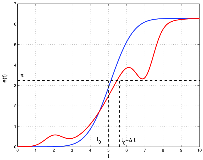
Figure 1: An example of two trajectories in $\mathcal{C}^{1}(t_{0}=5)$

3 The MTLL in the optimal smoother

The Wentzell-Freidlin theorem [8, 9] and the singular perturbation method [29] for asymptotic evaluation of the MTLL are concerned with stochastic processes satisfying a stochastic differential equation with a unique solution. In contrast, the dynamics of the optimal smoother, derived from the EL equations, form a two-point boundary-value problem which has no unique solution. Therefore the Wentzell-Freidlin and the singular perturbation method seem inappropriate for the computation of the MTLL in a smoother. It appears that this computation calls for a different approach.

The first step toward an asymptotic calculation of the MTLL in smoothers is the computation of the asymptotic distribution of the estimation error in case the number of trajectories in the optimization problem is finite. We investigate the cost functional of deterministic error trajectories that deviate from the original trajectory $\mbox{\boldmath$x$}(t)$. We augment $\mbox{\boldmath$x$}(t)$ with the set of the $N_{T}$ trajectories $\mbox{\boldmath$r$}_{i}(t)=[r_{i}(t),r_{i}^{[2]}(t),\ldots,r_{i}^{[N]}(t)]\in\mathscr{C}^{N}_{[0,T]},\ i\in[1,\ldots,N_{T}]$. The trajectories $\mbox{\boldmath$x$}(t)+\mbox{\boldmath$r$}_{i}(t)$ are admissible in the optimization problem (5), (6), only if the trajectories $\mbox{\boldmath$r$}_{i}(t)$ satisfy

$$\dot{\mbox{\boldmath$r$}}_{i}=\mbox{\boldmath$A$}\mbox{\boldmath$r$}_{i}+\mbox{\boldmath$B$}\mbox{\boldmath$u$}_{i}.$$ (10)

We define the difference

$$\Delta J[\mbox{\boldmath$x$}(\cdot),\mbox{\boldmath$r$}_{i}(\cdot)]\stackrel{{\scriptstyle\triangle}}{{=}}J[\mbox{\boldmath$x$}(\cdot)+\mbox{\boldmath$r$}_{i}(\cdot)]-J[\mbox{\boldmath$x$}(\cdot)]$$ (11)

and substitute (5), (6) and (10) in (11) to obtain

$$\begin{array}[]{lll}\Delta J[\mbox{\boldmath$x$}(\cdot),\mbox{\boldmath$r$}_{i}(\cdot)]&=&\displaystyle\int_{0}^{T}{\left[4\sin^{2}\left(\displaystyle\frac{r_{i}}{2}\right)+|\mbox{\boldmath$u$}_{i}|^{2}\right]}\,dt\\ &&\\ &+&\sqrt{4\,\varepsilon}\displaystyle\int_{0}^{T}{\left[\sin x-\sin(x+r_{i})\right]}\,dv_{1}(t)\\ &&\\ &+&\sqrt{4\,\varepsilon}\displaystyle\int_{0}^{T}{\left[\cos x-\cos(x+r_{i})\right]}\,dv_{2}(t)\\ &&\\ &+&\sqrt{4\,\varepsilon}\displaystyle\int_{0}^{T}\mbox{\boldmath$u$}_{i}^{T}\,d\mbox{\boldmath$w$}(t).\end{array}$$ (19)

At this point, we take the white noise limit in the wide band noises so the stochastic integrals in (19) become Itô integrals. Collecting them into a single Itô integral leads to

$$\begin{array}[]{lll}\Delta J[\mbox{\boldmath$x$}(\cdot),\mbox{\boldmath$r$}_{i}(\cdot)]&=&\displaystyle\int_{0}^{T}\left[4\sin^{2}\left(\displaystyle\frac{r_{i}}{2}\right)+|\mbox{\boldmath$u$}_{i}|^{2}\right]\,dt\\ &&\\ &+&\sqrt{4\,\varepsilon}\displaystyle\int_{0}^{T}\sqrt{4\sin^{2}\left(\displaystyle\frac{r_{i}}{2}\right)+|\mbox{\boldmath$u$}_{i}|^{2}}\,\,d\tilde{v}_{i}(t),\end{array}$$ (23)

where $\tilde{v}_{i}(t)$ is a standard Brownian motion that depends on $\mbox{\boldmath$v$}(t)$ and $\mbox{\boldmath$w$}(t)$.

Note that although the values of the random variable $\Delta J[\mbox{\boldmath$x$}(\cdot),\mbox{\boldmath$r$}_{i}(\cdot)]$ depend on the trajectories of $\mbox{\boldmath$x$}(t)$ and $\mbox{\boldmath$y$}(t)$ through $\mbox{\boldmath$v$}(t)$ and $\mbox{\boldmath$w$}(t)$, the probability law of $\Delta J[\mbox{\boldmath$x$}(\cdot),\mbox{\boldmath$r$}_{i}(\cdot)]$ depends only on the trajectories $\mbox{\boldmath$r$}_{i}(t)$. Therefore, we abbreviate notation to $\Delta J[\mbox{\boldmath$r$}_{i}(\cdot)]$. We note further that $\Delta J[\mbox{\boldmath$r$}_{i}(\cdot)]$ is a Gaussian random variable with expectation

$$\mbox{E}\Delta J[\mbox{\boldmath$r$}_{i}(\cdot)]=m_{i},$$ (24)

where

$$m_{i}\stackrel{{\scriptstyle\triangle}}{{=}}\int_{0}^{T}\left[4\sin^{2}\left(\displaystyle\frac{r_{i}}{2}\right)+|\mbox{\boldmath$u$}_{i}|^{2}\right]\,dt,$$ (25)

and variance

$$\mbox{Var}\{\Delta J[\mbox{\boldmath$r$}_{i}(\cdot)]\}=4\varepsilon\,m_{i}.$$ (26)

Furthermore, we compute the covariance

$$\begin{array}[]{lll}\sigma_{i\,j}&=&\mbox{E}\left(\Delta J[\mbox{\boldmath$r$}_{i}(\cdot)]-m_{i}\right)\left(\Delta J[\mbox{\boldmath$r$}_{j}(\cdot)]-m_{j}\right)\\ &&\\ &=&4\varepsilon\displaystyle\int_{0}^{T}\mbox{\boldmath$u$}_{i}^{T}\mbox{\boldmath$u$}_{j}\,dt+4\varepsilon\displaystyle\int_{0}^{T}\left[1+\cos(r_{i}-r_{j})-\cos r_{i}-\cos r_{j}\right]\,dt.\end{array}$$ (30)

Note that if the supports of $\mbox{\boldmath$r$}_{i}(\cdot)$ and $\mbox{\boldmath$r$}_{j}(\cdot)$ are disjoint, the cost functionals $\Delta J[\mbox{\boldmath$r$}_{i}(\cdot)],\,$ $\Delta J[\mbox{\boldmath$r$}_{j}(\cdot)]$ are not correlated. We conclude that the random variables $\Delta J[\mbox{\boldmath$r$}_{i}(\cdot)],\ i=1\ldots N_{T}$, form a Gaussian random vector with distribution

$$\left[\begin{array}[]{c}\Delta J[\mbox{\boldmath$r$}_{1}(\cdot)]\\ \\ \Delta J[\mbox{\boldmath$r$}_{2}(\cdot)]\\ \\ \vdots\\ \\ \Delta J[\mbox{\boldmath$r$}_{N_{T}}(\cdot)]\\ \end{array}\right]\sim N\left\{\left[\begin{array}[]{c}m_{1}\\ \\ m_{2}\\ \\ \vdots\\ \\ m_{N_{T}}\\ \end{array}\right]\ ;\ 4\,\varepsilon\left[\begin{array}[]{cccc}m_{1}&\sigma_{1\,2}&\ldots&\tilde{\sigma}_{1\,N_{T}}\\ &&&\\ \tilde{\sigma}_{1\,2}&m_{2}&&\\ &&&\\ \vdots&&\ddots&\\ &&&\\ \tilde{\sigma}_{1\,N_{T}}&&&m_{N_{T}}\\ \end{array}\right]\right\},$$ (52)

where $\tilde{\sigma}_{ij}=\displaystyle\frac{1}{4\,\varepsilon}\sigma_{ij}$.

When considering a finite number of error trajectories $\mbox{\boldmath$r$}_{i}(\cdot),\,i=1,\ldots,N_{T}$ in the optimization problem. The estimator error trajectory $\mbox{\boldmath$e$}_{N_{T}}(\cdot)$ minimizes the cost functional $\Delta J[\mbox{\boldmath$r$}_{j}(\cdot)]$,

$$\Pr\left\{\mbox{\boldmath$e$}_{N_{T}}(\cdot)=\mbox{\boldmath$r$}_{k}(\cdot)\right\}=\Pr\left\{\Delta J[\mbox{\boldmath$r$}_{k}(\cdot)]<\Delta J[\mbox{\boldmath$r$}_{j}(\cdot)]\,\mbox{for all}\ j\neq k\right\}.$$ (53)

Thus the problem of minimization has been recast in the language of order statistics. The probability on the right side of (53) is difficult to calculate, so we pursue the distribution of the error trajectory $\mbox{\boldmath$e$}_{N_{T}}(\cdot)$ in the limit of small $\varepsilon$. We assume that for each $k$ there exists an interval $A_{k}$ such that

$$\mbox{E}\left\{\Delta J[\mbox{\boldmath$r$}_{j}(\cdot)]\,|\,\Delta J[\mbox{\boldmath$r$}_{k}(\cdot)\in A_{k}]\right\}>\Delta J[\mbox{\boldmath$r$}_{k}(\cdot)]\quad\mbox{for all}\quad j\neq k.$$ (54)

Cramér’s theorem for Gaussian vectors [8, 7] implies that in the limit of small $\varepsilon$

$$\begin{array}[]{lll}&&\displaystyle\lim_{\varepsilon\to 0}\varepsilon\log_{e}\Pr\left\{\Delta J[\mbox{\boldmath$r$}_{k}(\cdot)]<\Delta J[\mbox{\boldmath$r$}_{j}(\cdot)]\quad\mbox{for all}\quad j\neq k\right\}=\\ &&\\ &&\displaystyle\lim_{\varepsilon\to 0}\varepsilon\log_{e}\Pr\left\{\Delta J[\mbox{\boldmath$r$}_{k}(\cdot)]\in A_{k}\right\}.\end{array}$$ (58)

Next, we evaluate the conditional expectation

$$\mbox{E}\left\{\Delta J[\mbox{\boldmath$r$}_{j}(\cdot)]\,|\,\Delta J[\mbox{\boldmath$r$}_{k}(\cdot)]\right\}.$$ (59)

Since $\Delta J[\mbox{\boldmath$r$}_{j}(\cdot)],\,\Delta J[\mbox{\boldmath$r$}_{k}(\cdot)]$ are jointly Gaussian,

$$\begin{array}[]{lll}\mbox{E}\left\{\Delta J[\mbox{\boldmath$r$}_{j}(\cdot)]\,|\,\Delta J[\mbox{\boldmath$r$}_{k}(\cdot)]\right\}&=&m_{j}+\displaystyle\frac{\sigma_{jk}}{4\,\varepsilon m_{k}}\left(\Delta J[\mbox{\boldmath$r$}_{k}(\cdot)]-m_{k}\right)\\ &&\\ &=&m_{j}+\displaystyle\frac{\tilde{\sigma}_{jk}}{m_{k}}\left(\Delta J[\mbox{\boldmath$r$}_{k}(\cdot)]-m_{k}\right).\end{array}$$ (63)

In order to determine the interval $A_{k}$, defined in (54), we derive the set of $N_{T}-1$ inequalities

$$\mbox{E}\left\{\Delta J[\mbox{\boldmath$r$}_{j}(\cdot)]\,|\,\Delta J[\mbox{\boldmath$r$}_{k}(\cdot)]\right\}>\Delta J[\mbox{\boldmath$r$}_{k}(\cdot)]\ \mbox{for all}\ j\neq k.$$ (64)

The interval $A_{k}$, which is the range of values of $\Delta J[\mbox{\boldmath$r$}_{k}(\cdot)]$ satisfying (64) is defined by

$$\mathop{\max}\limits_{\mbox{\boldmath$r$}_{j}(\cdot)\in A^{-}}\frac{m_{j}-\tilde{\sigma}_{jk}}{1-\displaystyle\frac{\tilde{\sigma}_{jk}}{m_{k}}}<\Delta J[\mbox{\boldmath$r$}_{k}(\cdot)]<\mathop{\min}\limits_{\mbox{\boldmath$r$}_{j}(\cdot)\in A^{+}}\frac{m_{j}-\tilde{\sigma}_{jk}}{1-\displaystyle\frac{\tilde{\sigma}_{jk}}{m_{k}}},$$ (65)

where $A^{+}$ is the set of all trajectories $\mbox{\boldmath$r$}_{j}(\cdot)$ such that $m_{j}<m_{k},\ \tilde{\sigma}_{jk}>m_{j}$, and $A^{-}$ is the set of all trajectories $\mbox{\boldmath$r$}_{j}(\cdot)$ such that $m_{j}>m_{k},\ \tilde{\sigma}_{jk}>m_{k}$. Note that the supremum and infimum, over all continuous trajectories, of the leftmost and rightmost sides of (65), respectively, is $-m_{k}$. This means that as $N_{T}$ increases and the trajectories $\mbox{\boldmath$x$}(\cdot)+\mbox{\boldmath$r$}_{i}(\cdot)$ are sampled from ${\mathscr{C}}_{[0,T]}$ according to their a priori distribution (3), the interval $A_{k}$ narrows. Specifically, for any $\delta,\,\tilde{\delta}>0$ there is a sufficiently large $N_{T}$ such that $\Pr\left\{A_{k}\not\subset(-m_{k}-\delta,-m_{k}+\delta)\right\}<\tilde{\delta}$. Combining (53) and (58), we conclude that for all small $\varepsilon>0$ and every sufficiently small $\delta$, such that $0<\delta<\varepsilon$, there is a sufficiently large $N_{T}$ such that

$$\begin{array}[]{lll}\Pr\left\{\mbox{\boldmath$e$}_{N_{T}}(\cdot)=\mbox{\boldmath$r$}_{k}(\cdot)\right\}&\asymp&\Pr\left\{-m_{k}-\delta<\Delta J[\mbox{\boldmath$r$}_{k}(\cdot)]<-m_{k}+\delta\right\}\\ &&\\ &\asymp&2\delta\exp\left\{-\displaystyle\frac{4\,m_{k}^{2}}{8\varepsilon\,m_{k}}\right\}\\ &&\\ &\asymp&2\delta\exp\left\{-\displaystyle\frac{1}{2\varepsilon}\displaystyle\int_{0}^{T}\left[4\sin^{2}\left(\displaystyle\frac{r_{k}}{2}\right)+|\mbox{\boldmath$u$}_{k}|^{2}\right]\,dt\right\}.\end{array}$$ (71)

Based on the distribution of the estimation error $\mbox{\boldmath$e$}_{N_{T}}(\cdot)$ in the case of a finite number of error trajectories $N_{T}$ (71), the probability that $\mbox{\boldmath$e$}_{N_{T}}(\cdot)$ is in any set $\mathscr{A}$ in $\mathscr{C}^{N}_{[0,T]}$ is

$$\begin{array}[]{lll}\Pr\left\{\mbox{\boldmath$e$}_{N_{T}}(\cdot)\in\mathscr{A}\right\}&=&\displaystyle\sum_{\mbox{\boldmath$r$}_{k}(\cdot)\in\mathscr{A}}\Pr\left\{\mbox{\boldmath$e$}_{N_{T}}(\cdot)=\mbox{\boldmath$r$}_{k}(\cdot)\right\}\\ &&\\ &\asymp&\displaystyle\sum_{\mbox{\boldmath$r$}_{k}(\cdot)\in\mathscr{A}}2\delta\exp\left\{-\displaystyle\frac{1}{2\varepsilon}\displaystyle\int_{0}^{T}\left[4\sin^{2}\left(\displaystyle\frac{r_{k}}{2}\right)+|\mbox{\boldmath$u$}_{k}|^{2}\right]\,dt\right\}.\end{array}$$ (75)

Applying Laplace’s method for sums of exponentials with large parameter $\displaystyle\frac{1}{\varepsilon}$ [3], we obtain the asymptotic expression

$$\Pr\left\{\mbox{\boldmath$e$}_{N_{T}}(\cdot)\in\mathscr{A}\right\}\asymp\exp\left\{-\displaystyle\frac{1}{2\varepsilon}\mathop{\min}\limits_{\mbox{\boldmath$r$}_{k}(\cdot)\in\mathscr{A}}\displaystyle\int_{0}^{T}\left[4\sin^{2}\left(\displaystyle\frac{r_{k}}{2}\right)+|\mbox{\boldmath$u$}_{k}|^{2}\right]\,dt\right\}.$$ (76)

In the limit $\delta\to 0$ (and $N_{T}\to\infty$), the probability that the optimal estimation error $\mbox{\boldmath$e$}(\cdot)$ is in $\mathscr{A}$ is found as

$$\Pr\left\{\mbox{\boldmath$e$}(\cdot)\in\mathscr{A}\right\}\asymp\exp\left\{-\displaystyle\frac{1}{2\varepsilon}\mathop{\inf}\limits_{\mbox{\boldmath$r$}(\cdot)\in\mathscr{A}}\displaystyle\int_{0}^{T}\left[4\sin^{2}\left(\displaystyle\frac{r}{2}\right)+|\mbox{\boldmath$u$}|^{2}\right]\,dt\right\},$$ (77)

subject to the equality constraint

$$\dot{\mbox{\boldmath$r$}}=\mbox{\boldmath$Ar$}+\mbox{\boldmath$Bu$},$$ (78)

where the infimum in (77) is taken over all continuous trajectories $\mbox{\boldmath$r$}(\cdot)\in\mathscr{A}$. Note that the small $\varepsilon$ approximation is taken before the limit $\delta\to 0.$

We turn now to the computation of the MTLL. First, we consider time intervals $[0,T]$ much longer than the time constant of the system, so that most of the time the system is in steady state. It follows that the probability $\Pr\left\{\mbox{slip in}\ (t_{0},t_{0}+\Delta t)\right\}$ is independent of $t_{0}$ for $t_{0}$ outside intervals of fixed length (the time constant of the system) at the endpoints $0$ and $T$. Therefore, in view of the regularity of the pdf of the solution as a function of $t$ and the independence of cycle slips in disjoint intervals (see above), for such $t_{0}$

$$\begin{array}[]{l}\Pr\left\{\mbox{slip in}\ (t_{0},t_{0}+2\Delta t)\right\}=\\ \\ \Pr\left\{\mbox{slip in}\ (t_{0},t_{0}+\Delta t)\right\}+\Pr\left\{\mbox{slip in}\ (t_{0}+\Delta t,t_{0}+2\Delta t)\right\}+o(\Delta t)=\\ \\ 2\Pr\left\{\mbox{slip in}\ (t_{0},t_{0}+\Delta t)\right\}+o(\Delta t).\end{array}$$ (84)

Thus, $\Pr\left\{\mbox{slip in}\ (t_{0},t_{0}+\Delta t)\right\}$ is nearly linear in $\Delta t$.

Next, we note that for fixed $\Delta t$ (77) implies that the slip probability satisfies

$$\begin{array}[]{lll}&&\Pr\left\{\mbox{slip in $(t_{0},t_{0}+\Delta t)$}\right\}\\ &&\\ &=&\Pr\left\{\mbox{\boldmath$e$}(\cdot)\in\mathscr{C}^{N}(t_{0})\right\}\\ &&\\ &\asymp&\exp\left\{-\displaystyle\frac{1}{2\varepsilon}\mathop{\inf}\limits_{\mbox{\boldmath$r$}(\cdot)\in\mathscr{C}^{N}(t_{0})}\displaystyle\int_{0}^{T}\left[4\sin^{2}\left(\displaystyle\frac{r}{2}\right)+|\mbox{\boldmath$u$}|^{2}\right]\,dt\right\},\end{array}$$ (90)

subject to the equality constraint (78). Equations (84) and (90) can be written together as

$$\begin{array}[]{lll}&&\\ &&\Pr\left\{\mbox{slip in $(t_{0},t_{0}+\Delta t)$}\right\}=\\ &&\\ &&(\Delta t+o(\Delta t))\Omega(\varepsilon)\exp\left\{-\mathop{\inf}\limits_{\mbox{\boldmath$r$}(\cdot)\in\mathscr{C}^{N}(t_{0})}\displaystyle\frac{1}{2\varepsilon}\displaystyle\int_{0}^{T}\left[4\sin^{2}\left(\displaystyle\frac{r}{2}\right)+|\mbox{\boldmath$u$}|^{2}\right]\,dt\right\},\\ &&\end{array}$$ (96)

subject to the equality constraint (78), where $\varepsilon\log\Omega(\varepsilon)\to 0$ as $\varepsilon\to 0$.

Equipped with the slip probability (96), we turn to the evaluation of the MTLL in the optimal smoother. We introduce a renewal (counting) process $\left\{\mathscr{N}(t),\,t\geq 0\right\}$, a nonnegative integer-valued stochastic process that counts the number successive cycle-slip events in the time interval $(0,t]$ [11]. We assume that the time durations between consecutive slips are positive, independent, identically distributed random variables. Based on the above assumptions, we adopt the renewal formula [11]

$$\tau_{nc}=\frac{t}{\mbox{E}\mathscr{N}(t)},$$ (97)

where $\tau_{nc}$ is the MTLL in the non-causal estimator. In the limit of $t\to\infty$, equation (97) gives

$$\tau_{nc}=\lim_{t\to\infty}\frac{t}{\mbox{E}\mathscr{N}(t)}=\lim_{t\to\infty}\frac{1}{\mbox{E}\dot{\mathscr{N}}(t)}.$$ (98)

Using the slip probability (96) we obtain

$$\begin{array}[]{lll}\mbox{E}\dot{\mathscr{N}}(t)&=&\displaystyle\lim_{\Delta t\to 0}\mbox{E}\left\{\displaystyle\frac{\mathscr{N}(t+\Delta t)-\mathscr{N}(t)}{\Delta t}\right\}\\ &&\\ &=&\displaystyle\lim_{\Delta t\to 0}\displaystyle\frac{\Pr\left\{\mbox{slip in}\ (t_{0},t_{0}+\Delta t)\right\}}{\Delta t}\\ &&\\ &\asymp&\exp\left\{-\mathop{\inf}\limits_{\mbox{\boldmath$r$}(\cdot)\in\mathscr{C}^{N}(t_{0})}\displaystyle\frac{1}{2\varepsilon}\displaystyle\int_{0}^{T}\left[4\sin^{2}\left(\displaystyle\frac{r}{2}\right)+|\mbox{\boldmath$u$}|^{2}\right]\,dt\right\}.\end{array}$$ (104)

Substituting (104) in (98), we obtain the expression for the asymptotic MTLL, $\tau_{nc}$, in the optimal MNE estimator

$$\lim_{\varepsilon\rightarrow 0}\varepsilon\log_{e}\tau_{nc}=\mathop{\inf}\limits_{\mbox{\boldmath$e$}(\cdot)\in\mathscr{C}^{N}(t_{0})}\frac{1}{2}\int_{0}^{T}\left[4\sin^{2}\left(\frac{e}{2}\right)+|\mbox{\boldmath$\xi$}|^{2}\right]\,dt,$$ (105)

subject to the equality constraint

$$\dot{\mbox{\boldmath$e$}}=\mbox{\boldmath$A$}\mbox{\boldmath$e$}+\mbox{\boldmath$B\xi$}.$$ (106)

4 The MTLL in the smoother with standard phase models

We begin with the first order phase tracking system suggested by [27] and [18], in which the phase $x(t)$ is modelled as a standard Brownian motion

$$\begin{array}[]{lll}&&\\ \dot{x}&=&\dot{w}\\ &&\\ y&=&\mbox{\boldmath$h$}(x)+\rho\,\dot{\mbox{\boldmath$v$}},\\ &&\end{array}$$ (112)

where $x(t),w(t)$ take values in $\mathbb{R}^{1}$. The system (112) is scaled to the form of (3), (4) with $\mbox{\boldmath$A$}=0,\mbox{\boldmath$B$}=1$ and $\varepsilon=\rho$. A similar procedure is presented in [4]. Note that the CNR equals $\rho^{-2}/2$ in the system (112).

In the first order case, the asymptotic expression for the MTLL in the smoother (105) becomes

$$\lim_{\varepsilon\rightarrow 0}\varepsilon\log_{e}\tau_{nc}=\mathop{\inf}\limits_{e(\cdot)\in\mathscr{C}^{1}(t_{0})}\frac{1}{2}\int_{0}^{T}\left[4\sin^{2}\left(\frac{e}{2}\right)+\dot{e}^{2}\right]\,dt,$$ (113)

The variational problem on the right side of (113) is solved analytically using the Hamilton-Jacobi-Belman equation [12]. This leads to the asymptotic limit of the MTLL in the first order non-causal estimator as

$$\lim_{\varepsilon\rightarrow 0}\varepsilon\log_{e}\tau_{nc}=\lim_{\rho\rightarrow 0}\rho\log_{e}\tau_{nc}=8.$$ (114)

In order to compare the MTLL in the optimal smoother (114) with that in the suboptimal PLL we construct the steady-state EKF corresponding to the model (112) [30].

$$\dot{\hat{x}}=\frac{\sigma}{\rho}\left(y_{s}\cos\hat{x}-y_{c}\sin\hat{x}\right).$$ (115)

The differential equation of the causal EKF estimation error $e(t)=\hat{x}(t)-x(t)$ is scaled to the form [4]

$$\dot{e}=-\sin e+\sqrt{2\varepsilon}\,\dot{v}.$$ (116)

The asymptotic MTLL, $\tau_{c}$, in this simple analytical potential case is known to be [29]

$$\lim_{\varepsilon\rightarrow 0}\varepsilon\log_{e}\tau_{c}=\lim_{\rho\rightarrow 0}\rho\log_{e}\tau_{c}=2.$$ (117)

Note that in first order estimators the MTLL in the non-causal estimator (114) is significantly longer than that in the causal estimator (117). This implies that the CNR values in the smoother are smaller than in the filter, but give a MTLL identical to that in the filter. Denoting by $\varepsilon_{c},\ \varepsilon_{nc}$ the values of $\varepsilon$ in the filter and smoother, respectively, and requiring identical MTLLs, lead to

$$\tau_{c}=\tau_{nc}\Rightarrow\frac{2}{\varepsilon_{c}}=\frac{8}{\varepsilon_{nc}}.$$ (118)

Denoting by $\mbox{CNR}_{c}[\mbox{dB}],\ \mbox{CNR}_{nc}[\mbox{dB}]$ the CNR in the filter and smoother, respectively, and using the simple relation between $\varepsilon$ and the CNR, lead to

$$\mbox{CNR}_{c}[\mbox{dB}]-\mbox{CNR}_{nc}[\mbox{dB}]=10\cdot 2\log_{10}(8/2)\approx 12\mbox{dB}.$$ (119)

Thus, there exists a 12dB performance gap in the MTLL between the estimators in terms of CNR. The MTLL in first order non-causal MNE smoother and causal EKF are given in Figures 2 and 3. The pre-exponential term in the plots is arbitrary.

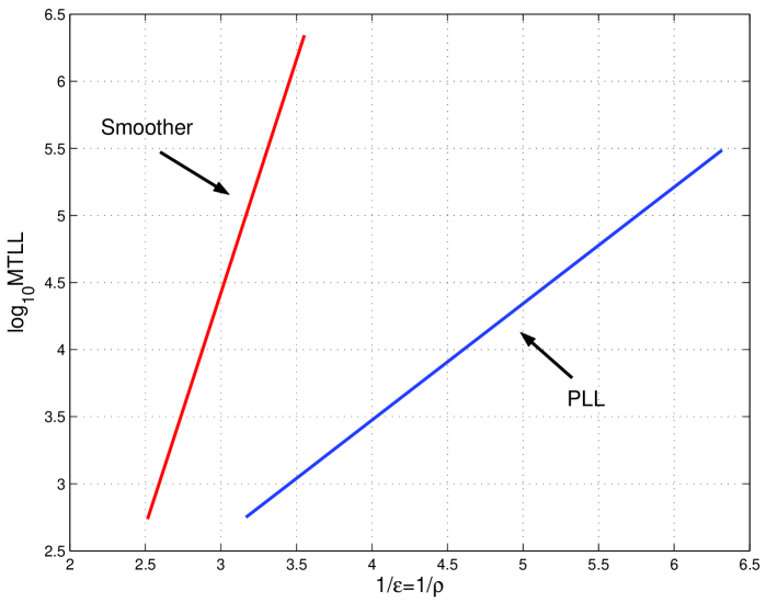
Figure 2: The MTLL in the first order optimal MNE estimator and the causal PLL as a function of $1/\varepsilon$.

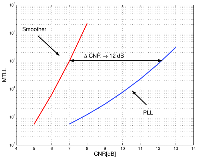
Figure 3: The MTLL in the first order optimal MNE estimator and the causal PLL as a function of the CNR.

Next we consider the more complex, and more realistic, case of a second order phase model [30], in which the phase is modelled as an integral over a Brownian motion. The signal model is

$$\dot{\mbox{\boldmath$x$}}=\mbox{\boldmath$A$}^{\prime}\mbox{\boldmath$x$}+\mbox{\boldmath$B$}^{\prime}\dot{\mbox{\boldmath$w$}},$$ (120)

where

$$\mbox{\boldmath$A$}^{\prime}=\left(\begin{array}[]{cc}0&1\\ 0&0\end{array}\right),\quad\mbox{\boldmath$B$}^{\prime}=\left(\begin{array}[]{cc}0&0\\ 0&1\end{array}\right).$$

The measurements model is

$$\mbox{\boldmath$y$}=\mbox{\boldmath$h$}(\mbox{\boldmath$x$})+\rho\,\dot{\mbox{\boldmath$v$}},$$ (122)

where $\mbox{\boldmath$x$}(t)$ and $\mbox{\boldmath$w$}(t)$ take values in $\mathbb{R}^{2}$. The system (120), (122) is scaled to the form of (3),(4) with $\mbox{\boldmath$A$}=\mbox{\boldmath$A$}^{\prime},\ \mbox{\boldmath$B$}=\mbox{\boldmath$B$}^{\prime}$, and $\varepsilon=\rho^{3/2}$. Note that in this case the CNR equals $\rho^{-2}/2$, as in the case of the first order system.

In the second order case, the asymptotic expression for the MTLL in the smoother (105) becomes

$$\lim_{\varepsilon\rightarrow 0}\varepsilon\log_{e}\tau_{nc}=\mathop{\inf}\limits_{e(\cdot)\in\mathscr{C}^{2}(t_{0})}\frac{1}{2}\int_{0}^{T}\left[4\sin^{2}\left(\frac{e}{2}\right)+\ddot{e}^{2}\right]\,dt,$$ (123)

variational problem on the right side of (105) as no analytical solution. An approximate solution is obtained numerically about the characteristics of the Hamilton-Jacobi-Belman equation [29, 5]. This leads to the asymptotic limit of the MTLL in the second order non-causal estimator as

$$\lim_{\varepsilon\rightarrow 0}\varepsilon\log_{e}\tau_{nc}=\lim_{\rho\rightarrow 0}\rho^{3/2}\log_{e}\tau_{nc}=5.$$ (124)

We note that the EKF corresponding to the second order system (120), (122) has the error equations [30],[5]

$$\begin{array}[]{lll}&&\\ \dot{e}&=&\displaystyle\frac{1}{2}\varphi-\sin e-\sqrt{2\varepsilon^{\prime}}\,\dot{v}\\ &&\\ \dot{\varphi}&=&-\sin e-\sqrt{2\varepsilon^{\prime}}\,\dot{v}+\sqrt{2\varepsilon^{\prime}}\,\dot{w},\\ &&\end{array}$$ (130)

where $\varepsilon^{\prime}=\varepsilon/\sqrt{2}$. The ”eikonal” equation [5] for the quasi-potential $\Phi$ corresponding to (130) is

$$\left(\frac{1}{2}\varphi-\sin e\right)\Phi_{e}-\sin e\,\Phi_{\varphi}+\Phi_{e}^{2}+2\Phi_{e}\Phi_{\varphi}+2\Phi_{\varphi}^{2}=0.$$ (131)

The function $\Phi$ is evaluated numerically on the characteristics of (131) [5]. This procedure leads to the value of the quasi-potential at the unstable equilibrium point $\Phi(\varphi=0,e=\pi)=0.6$, so the asymptotic MTLL in the second order causal estimator is

$$\lim_{\varepsilon\rightarrow 0}\varepsilon\log_{e}\tau_{c}=\lim_{\rho\rightarrow 0}\rho^{3/2}\log_{e}\tau_{c}=0.85.$$ (132)

Note that similarly to the first order case, the MTLL in the second order smoother (124) is significantly longer than that in the causal PLL (132). The CNR gap in this case is

$$\mbox{CNR}_{c}[\mbox{dB}]-\mbox{CNR}_{nc}[\mbox{dB}]=40/3\log_{10}(5/0.85)\approx 10.25\mbox{dB}.$$ (133)

The MTLL in the non-causal estimator and the causal EKF in the second order system are given in Figures 4 and 5. The pre-exponential term in the plots is arbitrary.

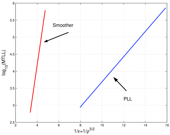
Figure 4: The MTLL in the second order optimal MNE estimator and the causal PLL as a function of $1/\varepsilon$.

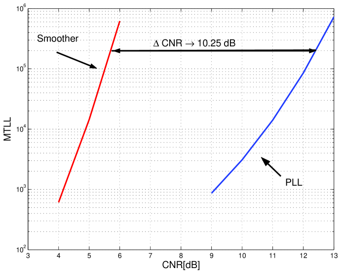
Figure 5: The MTLL in the second order optimal MNE estimator and the causal PLL as a function of CNR.

5 Discussion and conclusions

The significant advantage of the optimal smoother over the causal PLL defies intuition. It was customary to think that the MTLL advantage of the smoother is linked and proportional to the MSE advantage of the smoother [32]. We argue that the MSE in an estimator is not related to the MTLL. In order to demonstrate this idea we introduce the following error equation

$$\dot{e}=-2\sin\frac{e}{2}+\sqrt{\varepsilon}\,\dot{\tilde{v}}.$$ (134)

The MSE in the linearized version of (134) is identical to that in linearized version of the system

$$\dot{e}=-\sin e+\sqrt{\varepsilon}\,\dot{\tilde{v}}.$$ (135)

However, due to the difference in the potential barrier in the above systems, the asymptotical MTLL, $\tau_{1}$, in the system (134) satisfies

$$\lim_{\varepsilon\to 0}\varepsilon\log_{e}\tau_{1}=\frac{1}{2}\mathop{\inf}\limits_{\{e(0)=0,\ e(T^{\prime})=2\pi\}}\int_{0}^{T^{\prime}}\left(\dot{e}+2\sin\frac{e}{2}\right)^{2}\,dt=8,$$ (136)

while the MTLL, $\tau_{2}$, in the system (135) satisfies

$$\lim_{\varepsilon\to 0}\varepsilon\log_{e}\tau_{2}=4,$$ (137)

and is significantly shorter than $\tau_{1}$. Thus, we conclude that the MTLL advantage of the optimal smoother over the PLL is due to an entirely different functional and cannot be predicted by the MSE advantage of the smoother over the filter.

There is a fundamental mathematical difference between the causal and the non-causal cases. Both problems involve the minimization of a functional, similar to that of the Wentzell-Freidlin theory for causal systems. There is, however, a difference between the functionals in the two theories. While the functional in the causal case vanishes along the exiting trajectories from the boundary of the domain of attraction of the locked state to the next locked state [9], in the non-causal case the functional vanishes only at the locked states, so it has to be computed along the entire slip trajectory.

References

• [1] Anderson, B.D.O. Fixed interval smoothing for nonlinear continuous time systems. J. Info. Control, 20:294–300, 1972.
• [2] Bellman, R., Kalba, R., and Middelton, D. Dynamic programming, sequential estimation and sequential detection processes. Proc. Nat. Acad. Sci.U.S.A., 47:338 341, 1961.
• [3] Bender, C.M., and Orszag, S.A. Advanced Mathematical Methods for Scientists and Engineers. Springer, New York, 1999.
• [4] Bobrovsky, B.Z., and Schuss, Z. Singular perturbation in filtering theory. IFAC Workshop on singular perturbations in optimal control, pages 1439–1447, June 1978.
• [5] Bobrovsky, B.Z., and Schuss, Z. A singular perturbation method for the computation of the mean first passage time in a non linear filter. SIAM, 42(1):174–187, Feb. 1982.
• [6] Bryson, A.B., and Ho, Y.C. Applied Optimal Control. John Wiley, New York, 1975.
• [7] Bucklew, J.A. Large Deviation Techniques in Decision, Simulation and Estimation. Wiley, New York, 1990.
• [8] Dembo, A., and Zeitouni, O. Large Deviations Techniques and Applications. Jones and Bartlett, 1993.
• [9] Freidlin, M.A., and Wentzell, A.D. Random Perturbations of Dynamical Systems. Springer-Verlag, New York, 1984.
• [10] Kailath, T., and Frost, P. An innovation approach to least-squares estimation part II: Linear smoothing in addative white noise. IEEE Trans. Auto. Contronl, AC-13:655–660, 1968.
• [11] Karlin S., and Taylor, H.M. A First Course in Stochastic Processes. Academic Press, 1975.
• [12] Kirk D.E. Optimal Control Theory - an Introduction. Prentice-Hall, Inc., 1970.
• [13] Kushner, H.J. Dynamical equations for optimal nonlinear filtering. J. Diff. Equations, 2:179–190, 1967.
• [14] Lee, R.C.K. Optimal Estimation Idetification and Control. M.I.T. Press, 1964.
• [15] Leondes, C.T., Peller, J.B., and Stear, E.B. Nonlinear smoothing theory. IEEE Trans. Sys. Sci. Cyb., SSC-6:63–71, 1970.
• [16] Lindsey, W.C. Synchronization Systems in Communication and Control. Prentice-Hall, Englewood Cliffs, 1972.
• [17] Liptser, R.S., and Shiryayev, A.N. Statistics of Random Processes, volume I,II. Springer-Verlag, New York, 1977.
• [18] Macchi, O., and Scharf, L.L. A dynamic programming algorithm for phase estimation and data decoding on random phase channels. IEEE Trans. Info. Theory, IT-27(5):585–595, Sept. 1981.
• [19] Meditch, J.S. A survey of data smoothing for linear and nonlinear dynamic systems. Automatica, 9:151–160, 1973.
• [20] Proakis, J.G. Digital Communications. McGraw-Hill, 4th edition, 2001.
• [21] Rauch, H.E. Linear estimation of sampled stochastic processes with random parameters. Technical Report 2108, Stanford Electronics Labratory, Stanford University, California, 1962.
• [22] Rauch, H.E. Solutions to the linear smoothing problem. IEEE Tans. Auto. Control., AC-8:371–372, 1963.
• [23] Rauch, H.E., Tung, F., and Steibel, C.T. Maximum likelihood estimates of linear dynamic systems. AIAA J., 3:1445–1450, 1965.
• [24] Ryter, D., and Meyr, H. Theory of phase tracking systems of arbitrary order. IEEE Trans. Info. Theory, IT-24:1–7, 1978.
• [25] Sage, A.P. Maximum a posteriori filtering and smoothing algorithms. Int. J. Control, 11:171–183, 1970.
• [26] Sage, A.P., and Ewing, W.S. On filtering and smoothing algorithms for nonlinear state estimation. Int. J. Control, 11:1–18, 1970.
• [27] Scharf, L.L., Cox, D.D., and Masreleiz, C.J. Modulo $2\pi$ phase sequence estimation. IEEE Trans. Info. Theory, IT-26(5):615–620, Sept. 1980.
• [28] Schuss, Z. Singular perturbation methods in stochastic differential equations of mathematical physics. SIAM, Rev 22:119–155, 1980.
• [29] Schuss, Z. Theory and Applications of Stochastic Differential Equations. John Wiley, New York, 1980.
• [30] Snyder, D.L. The State Variable Approach to Continuous Estimation. The M.I.T Press, 1969.
• [31] Tausworth, R. Cycle slipping in phase locked loops. IEEE Trans. Comm., COM-15:417–421, 1967.
• [32] Van Trees, H.L. Detection, Estimation and Modulation Theory, volume II. John Wiley, New York, 1970.
• [33] Viterbi, A.J. Principles of Coherent Communication. McGraw-Hill, New York, 1966.
• [34] Viterbi, A.J., and Omura, J.K. Principles of Digital Communication and Coding. McGraw-Hill, 1979.
• [35] Weaver, C.S. Estimating the output of a linear discrete system with Gaussian input. IEEE Trans. Auto. Control, AC-8:372–374, 1963.