Adiabatic charge and spin pumping through quantum dots with ferromagnetic leads

Abstract

We study adiabatic pumping of electrons through quantum dots attached to ferromagnetic leads. Hereby we make use of a real-time diagrammatic technique in the adiabatic limit that takes into account strong Coulomb interaction in the dot. We analyze the degree of spin polarization of electrons pumped from a ferromagnet through the dot to a nonmagnetic lead (N-dot-F) as well as the dependence of the pumped charge on the relative leads’ magnetization orientations for a spin-valve (F-dot-F) structure. For the former case, we find that, depending on the relative coupling strength to the leads, spin and charge can, on average, be pumped in opposite directions. For the latter case, we find an angular dependence of the pumped charge, that becomes more and more anharmonic for large spin polarization in the leads.

I Introduction

Charge and spin transport through a nanoscale conductor can be obtained, in the absence of a transport voltage, by periodically varying in time some of its parameters. If the time dependence of the system is slow compared to its characteristic response time, we refer to this transport mechanism as adiabatic pumping. This particular regime allows us to study the properties of a system being slightly out of equilibrium due to an explicit time-dependence of its parameters. Numerous works have studied mesoscopic pumps both theoretically brouwer98 ; zhou99 ; buttiker01 ; buttiker02 ; entin02 as well as experimentally.switkes99 ; pothier92 ; geerligs91 ; fletcher03 ; watson03 The established framework to calculate the pumped charge through a mesoscopic scatterer is based on the dynamical scattering approach.buttiker94 ; brouwer98 This approach can be applied when the Coulomb interaction can be neglected or treated within the Hartree approximation. Recently, the interest in including the effects of Coulomb interaction beyond the Hartree level to the problem of adiabatic pumping has arisen.aleiner98 ; citro03 ; aono04 ; brouwer05 ; cota05 ; splett05 ; sela06 ; splett06 ; fioretto07

Spin-dependent transport through nanostructures has recently attracted a lot of interest. A model example is a quantum-dot spin valve, which consists of an interacting (single-level) quantum dot attached to two ferromagnetic leads (F-dot-F), see Fig. 1. The leads have, in general, non-collinear magnetization directions and different polarization strengths.

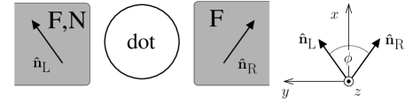
Figure 1: Schematic setup of N-dot-F or F-dot-F setup. The magnetization directions and the polarization strengths of the left and right lead can in general differ from each other (left). Sketch of the coordinate system and the magnetization directions of the leads (right).

Transport through a quantum-dot spin valve with noncollinear leads has been studied extensively in the dc limit.braun04 ; QDSV In magnetic multilayers the tunneling current depends chiefly on the relative orientation of the magnetization of the ferromagnetic layers.julliere75 ; slonczewski The situation is more complex in a quantum-dot spin valve due to the interplay of the lead magnetization, Coulomb interaction, non-equilibrium spin accumulation, and quantum fluctuations. In particular, a finite spin accumulation is generated on the dot, which plays an important role in determining charge transport.

In the present paper we combine the ideas of adiabatic pumping and spin-dependent transport through interacting nanostructures. We consider two scenarios. First, we focus on the situation when only one of the two leads is ferromagnetic (N-dot-F), for which we study the spin pumped into the non-magnetic lead. Spin pumping in systems where the spin degeneracy is lifted by a magnetic field has been the subject of several studies.mucciolo02 ; blaauboer03 ; watson03 ; aono04 ; sela06 Furthermore spin pumping by means of electrical gating only was predicted in a system with Rashba spin-orbit coupling.governale03 Several aspects of a noninteracting spin pump based on ferromagnets were studied in Ref. zheng03, . Spin pumping through an interface between a ferromagnet and a non-magnetic metal has been investigated in Ref. brataas02, , where the pumping cycle is realized exploiting the precession of the magnetization of the ferromagnet. In our setup we are interested in spin pumping obtained by varying periodically the properties of the scattering region, such as the dot level position and the tunneling strength to the left and the right lead, but leaving the lead properties, as e.g. their magnetizations, constant in time. A particular intriguing result for the system under consideration is that, depending on the relative coupling strength between dot and leads, spin and charge can on average be transported in opposite directions.

Second, we consider the case that both leads are spin polarized (F-dot-F). We study the influence of the spin polarizations of the leads on the pumped charge and on the average spin accumulated on the quantum dot during a pumping cycle. As a result, we find that also the pumped charge displays the spin-valve effect, i.e., a dependence on the relative angle between magnetization direction of the leads. For stronger spin polarization of the leads, the pumped charge becomes a more and more anharmonic function of the relative angle.

In order to calculate the charge and the spin pumped through the dot we use real-time diagrammatic technique in the adiabatic limit koenig96 ; splett06 and perform a rigorous perturbation expansion in the tunnel coupling to the leads. We consider the system in the regime of weak coupling, considering only first-order processes in the tunnel-coupling strengths.

II Model and Formalism

II.1 Hamiltonian

We consider a single-level quantum dot contacted by tunnel barriers to two ferromagnetic leads with different spin polarization axes, as shown in Fig. 1. For finite spin polarization in both leads (F-dot-F), the system is called a quantum-dot spin valve. The limit of one normal and one ferromagnetic lead (N-dot-F) is included by setting the spin polarization of one lead to zero. The total Hamiltonian of the system can be written as

$$H=H_{\mathrm{dot}}+\sum_{\alpha=\mathrm{L,R}}H_{\mathrm{lead,\alpha}}+H_{\mathrm{tunnel}}\ .$$ (1)

It consists of the Hamilton operators for the dot, for the left (L) and right (R) lead and for electron tunneling between dot and leads. The single-level quantum dot is described by the Hamiltonian

$$H_{\mathrm{dot}}=\sum_{\sigma=\uparrow,\downarrow}\epsilon_{\sigma}(t)n_{\sigma}+Un_{\uparrow}n_{\downarrow}\ ,$$ (2)

where the operator $d^{\dagger}_{\sigma}(d_{\sigma})$ creates (annihilates) an electron with spin $\sigma=\uparrow,\downarrow$ on the dot and $n_{\sigma}=d^{\dagger}_{\sigma}d_{\sigma}$ is the number operator for electrons with spin $\sigma$. The strength of the Coulomb interaction between electrons on the dot is denoted by $U$, which can be arbitrarily large. The energy level $\epsilon_{\sigma}(t)=\bar{\epsilon}_{\sigma}+\delta\epsilon_{\sigma}(t)$ of the dot can vary in time. In the following, we assume the dot level to be spin degenerate, i.e. $\epsilon_{\uparrow}(t)=\epsilon_{\downarrow}(t)=\epsilon(t)$. The Hamiltonian of the lead $\alpha$, with $\alpha=\mathrm{L,R}$ is given by

$$H_{\mathrm{lead},\alpha}=\sum_{k\sigma}\epsilon_{k\sigma}c^{\dagger}_{\alpha k\sigma}c_{\alpha k\sigma}\,.$$ (3)

We choose the spin quantization axis of lead $\alpha$ along the direction of its magnetization, $\mathbf{\hat{n}}_{\alpha}$. The spin $\sigma$ of an electron in lead $\alpha$ can take the values $\sigma=\pm$, where $+$ refers to the majority spin and $-$ to the minority spin of this lead. We choose a coordinate system with the three basis vectors $\mathbf{\hat{e}}_{x}$, $\mathbf{\hat{e}}_{y}$ and $\mathbf{\hat{e}}_{z}$, pointing along $\mathbf{\hat{n}}_{\mathrm{L}}+\mathbf{\hat{n}}_{\mathrm{R}}$, $\mathbf{\hat{n}}_{\mathrm{L}}-\mathbf{\hat{n}}_{\mathrm{R}}$ and $\mathbf{\hat{n}}_{\mathrm{R}}\times\mathbf{\hat{n}}_{\mathrm{L}}$ respectively, in analogy to the definition in Ref. braun04, . The angle between the spin quantization axis of the left lead, $\mathbf{\hat{n}}_{\mathrm{L}}$, and the spin quantization axis of the right lead, $\mathbf{\hat{n}}_{\mathrm{R}}$, is given by $\phi$. We show a sketch of the coordinate system and of the magnetization directions of the leads in Fig. 1. As spin quantization axis of the dot we take the $z$-axis of this coordinate system. With this choice the tunneling Hamiltonian reads

$$H_{\mathrm{tunnel}} = \frac{V_{\mathrm{L}}(t)}{\sqrt{2}}\sum_{k}\left[c^{\dagger}_{\mathrm{L}k+}\left(e^{i\phi/4}d_{\uparrow}+e^{-i\phi/4}d_{\downarrow}\right)\right.$$

$$\left.+c^{\dagger}_{\mathrm{L}k-}\left(-e^{i\phi/4}d_{\uparrow}+e^{-i\phi/4}d_{\downarrow}\right)\right]$$

$$+ \frac{V_{\mathrm{R}}(t)}{\sqrt{2}}\sum_{k}\left[c^{\dagger}_{\mathrm{R}k+}\left(e^{-i\phi/4}d_{\uparrow}+e^{i\phi/4}d_{\downarrow}\right)\right.$$

$$\left.+c^{\dagger}_{\mathrm{R}k-}\left(-e^{-i\phi/4}d_{\uparrow}+e^{i\phi/4}d_{\downarrow}\right)\right]+\mathrm{h.c.}$$

The tunnel matrix elements, $V_{\mathrm{L}}(t)$ and $V_{\mathrm{R}}(t)$, can be both time dependent. The generalized tunnel rates are defined by $\Gamma_{\alpha}\left(t,t^{\prime}\right)=\frac{1}{2}\sum_{\sigma=\pm}2\pi V^{*}_{\alpha}\left(t\right)V_{\alpha}\left(t^{\prime}\right)\rho_{\alpha,\sigma}=\frac{1}{2}\sum_{\sigma=\pm}\Gamma_{\alpha,\sigma}\left(t,t^{\prime}\right)$ and $\Gamma_{\alpha}\left(t\right)=\Gamma_{\alpha}\left(t,t\right)$. Here $\rho_{\alpha,\sigma}$ is the density of states of the spin species $\sigma$ in lead $\alpha$, which is supposed to be constant. The spin polarization of lead $\alpha$ is defined as

$$p_{\alpha}=\frac{\rho_{\alpha+}-\rho_{\alpha-}}{\rho_{\alpha+}+\rho_{\alpha-}}\ ,$$ (5)

and it can take values between $0$ and $1$.

II.2 Real-time diagrammatic approach

The Hilbert space of the single-level quantum dot is four dimensional, and it is spanned by the states $\chi=0,\uparrow,\downarrow,d$ (empty dot, singly occupied dot with spin up, singly occupied dot with spin down, doubly occupied dot). On the other hand, the non-interacting leads attached to the dot have a large number of degrees of freedom and act as baths. Hence, we can trace them out to obtain an effective description of the quantum dot. The dot dynamics are fully described by its reduced density matrix, $\rho_{\mathrm{dot}}$, with matrix elements $P_{\chi_{2}}^{\chi_{1}}=\langle\chi_{2}|\rho_{\mathrm{dot}}|\chi_{1}\rangle$. We introduce also the notation $P_{\chi}=P_{\chi}^{\chi}$ for the diagonal matrix elements (probabilities). The time evolution of the reduced density matrix is governed by the generalized master equation

$$\frac{d}{dt}P^{\chi_{1}}_{\chi_{2}}\left(t\right) = -\frac{i}{\hbar}(E_{\chi_{1}}-E_{\chi_{2}})P^{\chi_{1}}_{\chi_{2}}\left(t\right)$$

$$+\sum_{\chi_{1}^{\prime},\chi_{2}^{\prime}}\int_{-\infty}^{t}dt^{\prime}W^{\chi_{1}\chi_{1}^{\prime}}_{\chi_{2}\chi_{2}^{\prime}}\left(t,t^{\prime}\right)P^{\chi_{1}^{\prime}}_{\chi_{2}^{\prime}}\left(t^{\prime}\right)\ .$$

The kernel $W^{\chi_{1}\chi_{1}^{\prime}}_{\chi_{2}\chi_{2}^{\prime}}\left(t,t^{\prime}\right)$ connects the states $\chi_{1}^{\prime}$ and $\chi_{2}^{\prime}$ at time $t^{\prime}$ with the states $\chi_{1}$ and $\chi_{2}$ at time $t$. It is useful to define the vector of the average occupation probabilities $\mathbf{P}=\left(P_{0},P_{1},P_{d}\right)=\left(P_{0},P_{\uparrow}+P_{\downarrow},P_{d}\right)$ and the spin expectation value, in units of $\hbar$, $\mathbf{S}=\left(S_{x},S_{y},S_{z}\right)$, whose components are given by

$$S_{x}=\frac{P^{\uparrow}_{\downarrow}+P^{\downarrow}_{\uparrow}}{2};\ S_{y}=i\frac{P^{\uparrow}_{\downarrow}-P^{\downarrow}_{\uparrow}}{2};\ S_{z}=\frac{P_{\uparrow}-P_{\downarrow}}{2}.$$ (7)

Since we consider spin-degenerate dot levels, $E_{\uparrow}=E_{\downarrow}$, we can drop the first term on the r.h.s. of Eq. (II.2).

We are concerned with adiabatic pumping, where no transport voltage is applied across the dot. The leads are therefore described by the same Fermi function $f(\omega)$. As a consequence, the instantaneous current through the dot vanishes, and we need to consider the first adiabatic correction in order to obtain the pumping current through the dot. We perform an adiabatic expansion along the lines of Ref. splett06, . We start by performing a Taylor expansion around the time $t$ of $\mathbf{P}(t^{\prime})$ appearing inside the integral on the r.h.s. of the generalized master equation

$$\frac{d}{dt}P^{\chi_{1}}_{\chi_{2}}\left(t\right) = \sum_{\chi_{1}^{\prime},\chi_{2}^{\prime}}\int_{-\infty}^{t}dt^{\prime}W^{\chi_{1}\chi_{1}^{\prime}}_{\chi_{2}\chi_{2}^{\prime}}\left(t,t^{\prime}\right)\left[P^{\chi_{1}^{\prime}}_{\chi_{2}^{\prime}}\left(t\right)\right.$$ (8)

$$\left.+\left(t^{\prime}-t\right)\frac{d}{dt}P^{\chi_{1}^{\prime}}_{\chi_{2}^{\prime}}\left(t\right)\right]\ .$$

This expansion is justified by the fact that the response time of the system is much smaller than the timescale of the parameter variation in time. We then expand the kernel itself as

$$W^{\chi_{1}\chi_{1}^{\prime}}_{\chi_{2}\chi_{2}^{\prime}}\left(t,t^{\prime}\right)\rightarrow\left(W^{\chi_{1}\chi_{1}^{\prime}}_{\chi_{2}\chi_{2}^{\prime}}\right)^{(i)}_{t}\left(t-t^{\prime}\right)+\left(W^{\chi_{1}\chi_{1}^{\prime}}_{\chi_{2}\chi_{2}^{\prime}}\right)^{(a)}_{t}\left(t-t^{\prime}\right).$$ (9)

The superscript $i(a)$ denotes the instantaneous contribution (its adiabatic correction). The instantaneous contribution corresponds to freezing all parameters to their values at time $t$, i.e. $X(\tau)\rightarrow X(t)$. The adiabatic correction is obtained by linearizing the time dependence of the parameters, i.e. $X(\tau)\rightarrow X(t)+(\tau-t)d/d\tau X(\tau)|_{\tau=t}$, and retaining only first-order terms in the time derivatives. Finally, we perform the adiabatic expansion of the elements of the reduced density matrix

$$P^{\chi_{1}}_{\chi_{2}}\left(t\right)\rightarrow\left(P^{\chi_{1}}_{\chi_{2}}\right)^{(i)}_{t}+\left(P^{\chi_{1}}_{\chi_{2}}\right)^{(a)}_{t}\ .$$ (10)

The subscript $t$ in Eqs. (9) and (10) denotes the time with respect to which the adiabatic expansion is performed. This time $t$ enters the respective quantities parametrically; both the instantaneous and the adiabatic correction to the kernel are functions of the time difference $(t-t^{\prime})$. At this stage, it is convenient to introduce the zero-frequency Laplace transform of the kernel as $\left(W^{\chi_{1}\chi_{1}^{\prime}}_{\chi_{2}\chi_{2}^{\prime}}\right)^{(i/a)}_{t}=\int_{-\infty}^{t}dt^{\prime}\left(W^{\chi_{1}\chi_{1}^{\prime}}_{\chi_{2}\chi_{2}^{\prime}}\right)^{(i/a)}_{t}(t-t^{\prime})$. In order to evaluate the kernel of the master equation we perform, on top of the adiabatic expansion, a perturbation expansion in the tunnel coupling $\Gamma$. In the following we take into account processes in first order in the tunnel coupling. This approach is valid in the weak-coupling limit, i.e. $k_{\mathrm{B}}T\gg\Gamma$. At the same time the condition for adiabaticity, $\Gamma\gg\Omega$, needs to be fulfilled. The instantaneous occupation probabilities and their adiabatic corrections obey the equations

$$0=\sum_{\chi_{1}^{\prime},\chi_{2}^{\prime}}\left(W^{\chi_{1}\chi_{1}^{\prime}}_{\chi_{2}\chi_{2}^{\prime}}\right)^{(i,1)}_{t}\left(P^{\chi_{1}^{\prime}}_{\chi_{2}^{\prime}}\right)^{(i,0)}_{t}$$ (11)

$$\frac{d}{dt}\left(P^{\chi_{1}}_{\chi_{2}}\right)^{(i,0)}_{t}=\sum_{\chi_{1}^{\prime},\chi_{2}^{\prime}}\left(W^{\chi_{1}\chi_{1}^{\prime}}_{\chi_{2}\chi_{2}^{\prime}}\right)^{(i,1)}_{t}\left(P^{\chi_{1}^{\prime}}_{\chi_{2}^{\prime}}\right)^{(a,-1)}_{t}.$$ (12)

The number in the superscripts designates the order in the perturbation expansion in the tunnel coupling. The fact that we find elements of the reduced density matrix in minus first order in the tunnel coupling is consistent with our perturbative scheme, as those terms are proportional to $\Omega/\Gamma$, which is small in the adiabatic limit. The evaluation of the matrix elements of the kernel is done using a real-time diagrammatic technique, which was developed in Ref. koenig96, , extended to systems containing ferromagnetic leads in Ref. braun04, , and extended to adiabatic pumping in Ref. splett06, . The adiabatic correction to the matrix elements of the kernel does not appear in lowest order in the tunnel coupling, as considered in this paper. The equations for the instantaneous probabilities and for the adiabatic correction to the probabilities can be summarized as

$$\hbar\frac{d}{dt}\left(\begin{array}[]{c}P_{0}\\ P_{1}\\ P_{d}\end{array}\right)=$$ (16)

$$\Gamma\left(\begin{array}[]{ccc}-2f(\epsilon)&1-f(\epsilon)&0\\ 2f(\epsilon)&-\left[1-f(\epsilon)+f(\epsilon+U)\right]&2\left[1-f(\epsilon+U)\right]\\ 0&f(\epsilon+U)&-2\left[1-f(\epsilon+U)\right]\end{array}\right)\left(\begin{array}[]{c}P_{0}\\ P_{1}\\ P_{d}\end{array}\right)+\left(\begin{array}[]{c}1-f(\epsilon)\\ -\left[1-f(\epsilon)-f(\epsilon+U)\right]\\ -f(\epsilon+U)\end{array}\right)\sum_{\alpha}2\Gamma_{\alpha}\mathbf{S}\cdot\mathbf{p}_{\alpha}\ .$$ (26)

Similarly, the equations for the expectation value of the spin read

$$\hbar\frac{d}{dt}\mathbf{S} = \left[f(\epsilon)P_{0}-\frac{1}{2}\left[1-f(\epsilon)-f(\epsilon+U)\right]P_{1}-\left[1-f(\epsilon+U)\right]P_{d}\right]\sum_{\alpha}\Gamma_{\alpha}\mathbf{p}_{\alpha}$$ (27)

$$- \Gamma\left[1-f(\epsilon)+f(\epsilon+U)\right]\mathbf{S}+\mathbf{S}\times\sum_{\alpha}\mathbf{B}_{\alpha}\ ,$$

where we introduced the notation $\mathbf{p}_{\alpha}=p_{\alpha}\mathbf{\hat{n}}_{\alpha}$. The interaction-induced exchange field or effective $B$-field appearing in Eq. (27) is given by the principal-value integral

$$\mathbf{B}_{\alpha}=\Gamma_{\alpha}\mathbf{p}_{\alpha}\int_{P}\frac{d\omega}{\pi}\left(\frac{1-f(\omega)}{\omega-\epsilon}+\frac{f(\omega)}{\omega-\epsilon-U}\right)\ .$$ (28)

The instantaneous elements of the reduced density matrix are obtained by setting the left hand side of Eqs. (16) and (27) to zero and by assigning superscripts $(i,0)$ to the vectors $\mathbf{P}$ and $\mathbf{S}$ on the right hand side of the equations. The first adiabatic corrections to the elements of the reduced density matrix are obtained by assigning to the vectors $\mathbf{P}$ and $\mathbf{S}$ the superscripts $(i,0)$ on the left hand side of the equations and the superscripts $(a,-1)$ on the right hand side.

III Results

Starting from the master equation we compute both the instantaneous matrix elements of the reduced density matrix and their first adiabatic correction. These are needed as an input for calculating the spin and charge current.

III.1 Dot occupation and spin

The fact that no transport voltage is applied to the system has important consequences on the occupation probabilities and the expectation value of the spin. To lowest order in the tunnel-coupling strength $\Gamma$, the instantaneous occupation probabilities are given by their equilibrium values, i.e. by the Boltzmann factors of the respective states

$$P_{\chi}^{(i,0)} = \frac{e^{-\beta E_{\chi}(t)}}{Z}\ ,$$ (29)

where $\beta=1/k_{\mathrm{B}}T$ is the inverse temperature, $E_{\chi}(t)$ the energy of the dot state $\chi$, and $Z$ the partition function. The spin expectation value vanishes,comment_equilibrium

$$\mathbf{S}^{(i,0)}=0\ .$$ (30)

When considering only first-order tunneling processes, the adiabatic correction to the reduced density matrix is linear in $\Omega/\Gamma$. While the spin polarization of the leads has no influence on the instantaneous probabilities, the situation is different for the adiabatic correction, which reads

$$\mathbf{P}^{(a,-1)}=-\frac{d\mathbf{P}^{(i,0)}}{dt}\tau_{\mathrm{rel}}^{Q}(t)\frac{\Gamma(t)^{2}}{\Gamma^{2}(t)-\left(\sum_{\alpha}\mathbf{p}_{\alpha}\Gamma_{\alpha}(t)\right)^{2}}\ ,$$ (31)

with the charge relaxation time given by $\tau_{\mathrm{rel}}^{Q}(t)$ with $\left(\tau_{\mathrm{rel}}^{Q}(t)\right)^{-1}=\Gamma(t)\left[1+f(\epsilon(t))-f(\epsilon(t)+U)\right]$ (the derivation of the expression for $\tau_{\mathrm{rel}}^{Q}$ is given in Appendix A.) For vanishing polarization in the two leads this result coincides with that obtained for an N-dot-N systemsplett06 ; comment_factor2

$$\mathbf{P}^{(a,-1)}=-\frac{d\mathbf{P}^{(i,0)}}{dt}\frac{1}{\Gamma(t)}\frac{1}{1+f(\epsilon(t))-f(\epsilon(t)+U)}\ .$$ (32)

We find non-vanishing contributions to the off-diagonal terms of the reduced density matrix, which vanish for zero polarization in the leads. The spin expectation value reads

$$\mathbf{S}^{(a,-1)}=\frac{1}{2}\frac{\partial\langle n\rangle^{(i,0)}(t)}{\partial t}\tau_{\mathrm{rel}}^{S}(t)\frac{\Gamma(t)\sum_{\alpha}\mathbf{p}_{\alpha}\Gamma_{\alpha}(t)}{\Gamma^{2}(t)-\left(\sum_{\alpha}\mathbf{p}_{\alpha}\Gamma_{\alpha}(t)\right)^{2}}\ ,$$ (33)

where the spin relaxation time $\tau_{\mathrm{rel}}^{S}(t)$ is given by $\left(\tau_{\mathrm{rel}}^{S}(t)\right)^{-1}=\Gamma(t)\left[1-f(\epsilon(t))+f(\epsilon(t)+U)\right]$ (the derivation of the expression for $\tau_{\mathrm{rel}}^{S}$ is given in Appendix A). Notice that the first adiabatic correction is the leading contribution to the expectation value of the dot spin. Furthermore, a time-dependent dot spin can be accumulated only by varying in time the occupation of the dot. The adiabatic correction to the spin component is parallel to the exchange field, introduced in Eq. (28). Therefore no precession of the spin around this field takes place. This is different from the case of a time-independent but biased spin valve.braun04

Finally, we remark that the limit where both leads are fully polarized along the same magnetization axis, $\phi=0$ and $p_{\mathrm{L}}=p_{\mathrm{R}}=1$ is ill defined; in fact, in this case the life time of a minority spin in the dot diverges and consequently in order for the adiabatic expansion to hold the pumping frequency needs to be zero.

III.2 Pumping Current

The results for the dot occupation probabilities and the expectation value of the spin on the dot serve to calculate the pumping current. Using a similar approach as for the generalized master equation we write the current into the left lead as

$$I_{\mathrm{L}}(t)=-e\int_{-\infty}^{t}dt^{\prime}\sum_{\chi_{1},\chi_{2},\chi_{1}^{\prime},\chi_{2}^{\prime}}\left(W_{\chi_{1}\chi_{1}^{\prime}}^{\chi_{2}\chi_{2}^{\prime}}\right)^{\mathrm{L}}(t,t^{\prime})P_{\chi_{1}^{\prime}}^{\chi_{2}^{\prime}}(t^{\prime})\ ,$$ (34)

where $\left(W_{\chi_{1}\chi_{1}^{\prime}}^{\chi_{2}\chi_{2}^{\prime}}\right)^{\mathrm{L}}(t,t^{\prime})=\sum_{q}q\left(W_{\chi_{1}\chi_{1}^{\prime}}^{\chi_{2}\chi_{2}^{\prime}}\right)^{\mathrm{L}q}(t,t^{\prime})$, and $\left(W_{\chi_{1}\chi_{1}^{\prime}}^{\chi_{2}\chi_{2}^{\prime}}\right)^{\mathrm{L}q}(t,t^{\prime})$ is the sum of all processes, describing transitions where the difference of the number of electrons entering and leaving the left lead is equal to the integer number $q$.

We compute the first order adiabatic correction to the current including only first-order tunneling processes. We find

$$I_{\mathrm{L}}^{(a,0)}(t) = -e\sum_{\chi_{1},\chi_{2},\chi_{1}^{\prime},\chi_{2}^{\prime}}\left(W_{\chi_{1}\chi_{1}^{\prime}}^{\chi_{2}\chi_{2}^{\prime}}\right)^{\mathrm{L}(i,1)}_{t}\left(P_{\chi_{1}^{\prime}}^{\chi_{2}^{\prime}}\right)^{(a,-1)}_{t}\ .$$

In the following we suppress the superscript $(a,0)$ for the current, since the instantaneous current is always zero and $I_{\mathrm{L}}^{(a,0)}(t)$ is therefore the dominant contribution. The current is of zeroth order in the tunnel coupling and proportional to the pumping frequency $\Omega$. To this order in the tunnel-coupling strengths, the pumped current is non-vanishing only if the dot level position is one of the pumping parameters, since $\left(P_{\chi_{1}^{\prime}}^{\chi_{2}^{\prime}}\right)^{(a,-1)}$ is proportional to the time derivative of the dot level position. We find for the pumping current

$$I_{\mathrm{L}} = -e\frac{\partial\langle n\rangle^{(i,0)}}{\partial t}\frac{\Gamma_{\mathrm{L}}(t)}{\Gamma(t)}$$ (35)

$$- e\frac{\partial\langle n\rangle^{(i,0)}}{\partial t}\frac{\Gamma_{\mathrm{L}}(t)\Gamma_{\mathrm{R}}(t)}{\Gamma(t)^{2}}\frac{\left(\mathbf{p}_{\mathrm{R}}-\mathbf{p}_{\mathrm{L}}\right)\boldsymbol{\pi}(t)}{1-\boldsymbol{\pi}(t)^{2}}\ ,$$

where we have defined the quantity $\boldsymbol{\pi}(t)=\sum_{\alpha}\Gamma_{\alpha}(t)\mathbf{p}_{\alpha}/\Gamma(t)=\sum_{\alpha}\boldsymbol{\pi}_{\alpha}(t)$, which depends on time via $\Gamma_{\alpha}(t)$. The pumped current consists of two terms of different origin: the first one is independent of the lead polarizations, and can be interpreted as arising from a peristaltic mechanism;splett06 the second term depends on the polarizations and can be seen as arising from the relaxation of the accumulated spin on the dot. The latter contribution due to spin relaxation can be either positive or negative depending on the polarization strengths, polarization directions and tunnel coupling to the different leads. This means that the time-resolved current can be enhanced with respect to the non-magnetic case, in contrast with the spin-valve effect in a time-independent system, which always leads to a current suppression. Similarly, we will see later that also the charge pumped through the dot per period is always suppressed due to the polarization of the leads. Therefore, this inverse spin-valve effect is observable only in the time-resolved current response. The effect could be investigated experimentally by means of time-resolved measurements or by rectifying the current response. Reduction or enhancement of the current can be achieved by tuning the tunnel coupling or the lead magnetizations.

III.3 N-dot-F: Spin Pumping

We now turn our attention to spin pumping in a setup where only one of the leads, the right one for the sake of definiteness, is ferromagnetic. We calculate the spin pumped in the unpolarized left lead.

The instantaneous contribution to the reduced density matrix is independent of the polarization and therefore remains unchanged. The first adiabatic correction for the occupation probabilities and the dot spin are given by Eq. (31) and Eq. (33), respectively, with $p_{\mathrm{L}}=0$.

The charge current through such a N-dot-F system can be obtained directly from Eq. (35) by setting $p_{\mathrm{L}}=0$ and it reads

$$I_{\mathrm{L}}=-e\frac{\partial\langle n\rangle^{(i,0)}}{\partial t}\frac{\Gamma(t)\Gamma_{\mathrm{L}}(t)}{\Gamma(t)^{2}-p_{\mathrm{R}}^{2}\Gamma_{\mathrm{R}}(t)^{2}}\ .$$ (36)

For calculating the spin current, we chose a global spin-quantization axis parallel to the magnetization of the right lead. In this basis the reduced density matrix does not have any off-diagonal terms. We find for the spin current

$$I_{\mathrm{L}}^{S}=\frac{\hbar}{2}\frac{\partial\langle n\rangle^{(i,0)}}{\partial t}\frac{\Gamma_{\mathrm{R}}(t)p_{\mathrm{R}}\Gamma_{\mathrm{L}}(t)}{\Gamma(t)^{2}-p_{\mathrm{R}}^{2}\Gamma_{\mathrm{R}}(t)^{2}}\ .$$ (37)

The ratio of the time-resolved spin and charge currents, Eq. (36) and Eq. (37), reads

$$\frac{I_{\mathrm{L}}^{S}}{I_{\mathrm{L}}}/\left[\frac{\hbar/2}{-e}\right] = \frac{p_{\mathrm{R}}\Gamma_{\mathrm{R}}(t)}{\Gamma(t)}.$$ (38)

This ratio is, in general, time dependent. The time-resolved spin current is smaller than the time-resolved particle current at any time $t$. The ratio of these two currents is always positive, implying that spin and charge flow in the same direction, as expected. The situation is different, for the spin (in units of $\hbar/2$) and the charge (in units of $-e$) pumped per period. We calculate the pumped charge and spin for the following two choices of pumping parameters, $\left\{\Gamma_{\mathrm{L}},\epsilon\right\}$ or $\left\{\Gamma_{\mathrm{R}},\epsilon\right\}$, in bilinear response, i.e. we calculate the pumped charge and spin per infinitesimal area in parameter space.

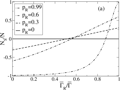
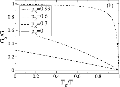
Figure 2: (a) Ratio of the pumped spin per period (in units of $\hbar/2$) to the pumped charge per period (in units of $-e$) as a function of the relative tunnel-coupling strength $\bar{\Gamma}_{\mathrm{R}}/\bar{\Gamma}$, for different polarizations of the right lead. (b) Ratio between the linear dc spin conductance and the linear dc conductance as a function of the relative tunnel-coupling strength $\bar{\Gamma}_{\mathrm{R}}/\bar{\Gamma}$, for different polarizations of the right lead.

The result for the ratio of the pumped spin (in units of $\hbar/2$) per period, $N_{S}$, and the pumped charge (in units of $-e$) per period, $N$, reads

$$\frac{N_{S}}{N} = -p_{\mathrm{R}}\frac{1+p_{\mathrm{R}}^{2}\left(\bar{\Gamma}_{\mathrm{R}}/\bar{\Gamma}\right)^{2}-2\left(\bar{\Gamma}_{\mathrm{R}}/\bar{\Gamma}\right)}{1+p_{\mathrm{R}}^{2}\left(\bar{\Gamma}_{\mathrm{R}}/\bar{\Gamma}\right)^{2}-2\left(\bar{\Gamma}_{\mathrm{R}}/\bar{\Gamma}\right)p_{\mathrm{R}}^{2}}\ .$$ (39)

It turns out that the efficiency of the spin pump does not depend on which pair of pumping parameters one chooses. In Fig. 2(a), we plot the ratio of pumped spin to pumped charge as a function of the relative tunnel-coupling strength ${\bar{\Gamma}_{\mathrm{R}}}/{\bar{\Gamma}}$, where the bar indicates time-averaged quantities, for different values of the polarization of the right lead. The absolute value of the ratio is maximally equal to one in the case of full polarization of the right lead. For $p_{\mathrm{R}}<1$, this ratio goes from $-p_{\mathrm{R}}$ for vanishing $\bar{\Gamma}_{\mathrm{R}}$ to $p_{\mathrm{R}}$ for vanishing $\bar{\Gamma}_{\mathrm{L}}$ changing its sign for

$$\frac{\Gamma_{\mathrm{R}}}{\Gamma}=\frac{1}{p_{\mathrm{R}}^{2}}\left(1-\sqrt{1-p_{\mathrm{R}}^{2}}\right)\ .$$ (40)

This is a very intriguing result, which implies that the respective direction in which spin and charge are pumped depends on the coupling to left and right lead.

The average pumped charge and the average pumped spin can have opposite signs, while the time-resolved spin and charge currents flow in the same direction at any instant of time, due to the fact that the ratio of the time-resolved currents, Eq. (38), is itself time dependent. To elucidate this, in Fig. 3, we plot the time-resolved spin and charge currents as a function of time for a configuration, where the pumped spin and charge per period have different signs. Note that the charge current has a positive average and the spin current has a negative average, while both currents flow in the same direction at any time.

We now contrast the results for the pumped spin and charge with the dc transport properties of the N-dot-F system. We find for the spin and charge currents

$$\frac{I^{S}}{I}/\left[\frac{\hbar/2}{-e}\right]=\frac{[1-f_{\mathrm{L}}(\epsilon)+f_{\mathrm{L}}(\epsilon+U)]\Gamma_{\mathrm{L}}p_{\mathrm{R}}}{[1-f_{\mathrm{L}}(\epsilon)+f_{\mathrm{L}}(\epsilon+U)]\Gamma_{\mathrm{L}}+[1-f_{\mathrm{R}}(\epsilon)+f_{\mathrm{R}}(\epsilon+U)]\Gamma_{\mathrm{R}}(1-p_{\mathrm{R}}^{2})}\ ,$$ (41)

which, in the linear response regime, yields for the ratio of the spin to the charge conductance

$$\frac{G^{S}}{G}/\left[\frac{\hbar/2}{-e}\right]=\frac{\Gamma_{\mathrm{L}}p_{\mathrm{R}}}{\Gamma_{\mathrm{L}}+\Gamma_{\mathrm{R}}(1-p_{\mathrm{R}}^{2})}\ .$$ (42)

The linear conductance ratio is shown in Fig. 2(b). Its behavior is completely different from that obtained by pumping. First, the spin polarization decreases as a function of $\bar{\Gamma}_{\mathrm{R}}/\bar{\Gamma}$ and, second, it stays always positive.

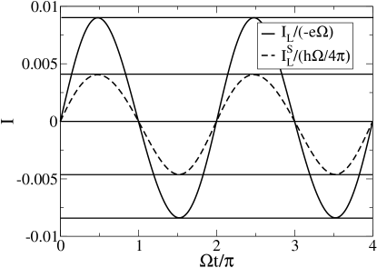
Figure 3: Time-resolved spin and charge currents as a function of time. The value of the parameters used for this plot are: $p_{\mathrm{R}}=0.99$,$\bar{\Gamma}_{\mathrm{L}}=\bar{\Gamma}_{\mathrm{R}}$, $\bar{\epsilon}=-\bar{\Gamma}$, $U=10\bar{\Gamma}$, $|\delta\Gamma_{\mathrm{L}}|/\bar{\Gamma}=|\delta\epsilon|/\bar{\Gamma}=0.1$ and $k_{\mathrm{B}}T=\bar{\Gamma}$.

Finally, we consider the spin accumulated on the dot in one pumping period. We find two different results depending on whether $\left\{\Gamma_{\mathrm{L}},\epsilon\right\}$ or $\left\{\Gamma_{\mathrm{R}},\epsilon\right\}$ are the pumping parameters:

$$\langle\mathbf{S}^{(a,-1)}\rangle_{T}\left(\left\{\Gamma_{\mathrm{L}},\epsilon\right\}\right)=-\frac{\eta}{\bar{\Gamma}}\frac{\partial\langle\bar{n}\rangle}{\partial\bar{\epsilon}}\bar{\tau}^{S}_{\mathrm{rel}}\frac{\bar{\boldsymbol{\pi}}_{\mathrm{R}}}{(1-\bar{\boldsymbol{\pi}}_{\mathrm{R}}^{2})^{2}}$$ (43)

$$\langle\mathbf{S}^{(a,-1)}\rangle_{T}\left(\left\{\Gamma_{\mathrm{R}},\epsilon\right\}\right)=\frac{\eta}{2\bar{\Gamma}}\frac{\partial\langle\bar{n}\rangle}{\partial\bar{\epsilon}}\bar{\tau}^{S}_{\mathrm{rel}}\frac{(\frac{\bar{\Gamma}_{\mathrm{L}}}{\bar{\Gamma}}-\frac{\bar{\Gamma}_{\mathrm{R}}}{\bar{\Gamma}})+\bar{\boldsymbol{\pi}}_{\mathrm{R}}^{2}}{(1-\bar{\boldsymbol{\pi}}_{\mathrm{R}}^{2})^{2}}\mathbf{p}_{\mathrm{R}}\ ,$$

where the area of the cycle in parameter space, $\eta$, is defined as $\eta=\int_{0}^{T}dt\frac{\partial\epsilon}{\partial t}\delta\Gamma_{\mathrm{L}}$ and $\eta=\int_{0}^{T}dt\frac{\partial\epsilon}{\partial t}\delta\Gamma_{\mathrm{R}}$ for the first and second equation respectively. In the case of pumping with $\left\{\Gamma_{\mathrm{R}},\epsilon\right\}$, i.e. when the coupling to the ferromagnetic lead is time dependent, the average spin changes sign at the same values of $\bar{\Gamma}_{\mathrm{R}}/\bar{\Gamma}$ at which the the ratio $I_{\mathrm{L}}^{\mathrm{S}}/I_{\mathrm{L}}$ changes its sign. On the contrary, when pumping with $\Gamma_{\mathrm{L}}$ and $\epsilon$, the average spin polarization of the dot does not change sign as a function of $\bar{\Gamma}_{\mathrm{R}}/\bar{\Gamma}$, while the ratio $I_{\mathrm{L}}^{\mathrm{S}}/I_{\mathrm{L}}$ still does.

III.4 F-dot-F: Spin-Valve Effect

We now consider the spin-valve setup with both leads having arbitrary spin polarizations. We compute the number of pumped charges per period, $N=-\frac{1}{e}\int_{0}^{T}dtI_{\mathrm{L}}(t)$, in bilinear response in the pumping parameters. For the pumping cycle defined by $\epsilon(t)=\bar{\epsilon}+\delta\epsilon(t)$ and $\Gamma_{\mathrm{L}}(t)=\bar{\Gamma}_{\mathrm{L}}+\delta\Gamma_{\mathrm{L}}(t)$, the number of pumped charges per period reads

$$N = \eta\frac{\partial\langle\bar{n}\rangle^{(i,0)}}{\partial\bar{\epsilon}}$$

$$\frac{\partial}{\partial\bar{\Gamma}_{\mathrm{L}}}\left(\frac{\bar{\Gamma}_{\mathrm{L}}\sum_{\alpha}\bar{\Gamma}_{\alpha}-\bar{\Gamma}_{\mathrm{L}}\mathbf{p}_{\mathrm{L}}\sum_{\alpha}\bar{\Gamma}_{\alpha}\mathbf{p}_{\alpha}}{\bar{\Gamma}^{2}-\left(\sum_{\alpha}\bar{\Gamma}_{\alpha}\mathbf{p}_{\alpha}\right)^{2}}\right)\ ,$$

with $\eta=\int_{0}^{T}dt\frac{\partial\epsilon}{\partial t}\delta\Gamma_{\mathrm{L}}$ being the area of the cycle in parameter space. Notice that the charge number in Eq. (III.4) is a product of two terms, where one contains effects of interactions and another one effects of the leads’ magnetization.

In the following we show results for the case that both leads have the same spin polarization strength. This corresponds to the experimentally relevant situation that both leads are realized with the same ferromagnetic material. In Fig. 4, we show the pumped charge as a function of the level position for different values of the angle between the directions of the magnetizations of the two leads. The pumped charge shows a peak when the energy $\bar{\epsilon}$ or $\bar{\epsilon}+U$ are close to the Fermi energy, similarly to pumping through a quantum dot contacted to two non-magnetic leads (N-dot-N).splett06 As far as the dependence on the angle between the magnetization of the two leads $\phi$ is concerned, for $\phi\in[0,\pi]$, the charge is monotonically suppressed for increasing $\phi$ until a minimum is reached for $\phi=\pi$ as in the usual dc spin-valve effect. The full $\phi$-dependence of the pumped charge is shown in Fig. 5, where we plot $N(\phi)/N(\phi=0)$. This result does not depend on the value of the level position and of the interaction strength, since the dependence on $\bar{\epsilon}$ and $U$ cancels out when we divide by $N(\phi=0)$. We notice that the suppression of charge pumping is stronger for higher lead polarizations. Furthermore, the more the lead polarization is increasing the stronger the behavior of the pumped charge as a function of the angle deviates from a cosine law.

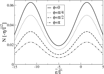
Figure 4: Pumped charge as a function of the average level position, $\bar{\epsilon}$, for different values of the angle between the magnetizations. The polarizations in the leads are $p_{\mathrm{L}}=p_{\mathrm{R}}=0.8$.

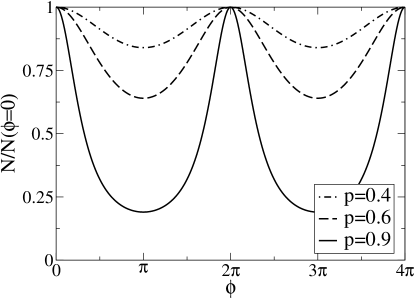
Figure 5: Pumped charge as a function of the angle between the magnetizations of the leads, $\phi$, for different polarization strengths $p_{\mathrm{L}}=p_{\mathrm{R}}=p$. This result does not depend on the level position and the interaction strength.

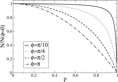
Figure 6: Pumped charge as a function of the polarization strength $p=p_{\mathrm{L}}=p_{\mathrm{R}}$, for different values of the angle between the magnetizations. This result does not depend on the level position and the interaction strength.

In Fig. 6, we show the pumped charge as a function of the lead polarization strengths for different values of the angle between the magnetization directions. This plot confirms that the pumped charge decreases for increasing spin polarization of the leads. The charge suppression is strongest when $\phi$ is near to $\pi$. Independently of the angle between the polarization axis of left and right lead, the pumped charge goes to zero for fully polarized leads. It is important to point out that this last property depends on the order in which limits are taken, since the two limits $\phi\rightarrow 0$ and $p_{\mathrm{L}}=p_{\mathrm{R}}\rightarrow 1$ do not commute, as was already mentioned in section III.1. In fact, comparing Fig. 5 and Fig. 6 we notice that in the first case the charge is maximal for $\phi=0$ even for the polarization increasing towards one, while in the second case for $p_{\mathrm{L}}=p_{\mathrm{R}}=1$, the charge is maximally suppressed even for $\phi$ going to zero.

The spin, which is accumulated on the dot during one pumping cycle is given by

$$\langle\mathbf{S}\rangle^{(a,-1)}_{T} = \frac{\eta}{2}\frac{\partial\langle\bar{n}\rangle^{(i,0)}}{\partial\epsilon}\bar{\tau}_{\mathrm{rel}}^{S}\left[\frac{\bar{\Gamma}\mathbf{p}_{\mathrm{L}}}{\bar{\Gamma}^{2}-\left(\sum_{\alpha}\mathbf{p}_{\alpha}\bar{\Gamma}_{\alpha}\right)^{2}}\right.$$

$$\left.-2\frac{\bar{\Gamma}^{2}-\bar{\Gamma}\mathbf{p}_{\mathrm{L}}\sum_{\alpha}\mathbf{p}_{\alpha}\bar{\Gamma}_{\alpha}}{\left(\bar{\Gamma}^{2}-\left(\sum_{\alpha}\mathbf{p}_{\alpha}\bar{\Gamma}_{\alpha}\right)^{2}\right)^{2}}\cdot\sum_{\alpha}\mathbf{p}_{\alpha}\bar{\Gamma}_{\alpha}\right],$$

where the pumping parameters are chosen to be $\Gamma_{\mathrm{L}}$ and $\epsilon$. The result for pumping with $\Gamma_{\mathrm{R}}$ and $\epsilon$ is easily obtained by swapping the indices L and R. Depending on the spin polarization of the leads and on the values of tunnel-coupling strengths, the average spin on the dot can point along any direction in the plane containing the magnetizations of the leads.

IV Conclusions

We have investigated adiabatic pumping through a single-level quantum dot with ferromagnetic leads in the regime of weak tunnel coupling between dot and leads, by means of a real-time diagrammatic approach. In the case that only one lead is ferromagnetic, we have computed the spin injected in the non-magnetic lead by pumping. We have found that, depending on the relative strength of the tunnel coupling to the leads, spin and charge can be pumped, on average, in opposite directions. For the case when both leads are polarized, we have found a suppression of the pumped charge by means of the spin-valve effect and determined the average spin accumulated on the dot during one pumping cycle.

Appendix A Relaxation times

In this appendix, we calculate the spin and charge relaxation times. In order to calculate the spin relaxation time, we consider the case when the charge on the dot is in equilibrium and the occupation probabilities are therefore given by the Boltzmann factors. Then Eq. (27) simplifies to

$$\frac{d\mathbf{S}}{dt}=-\Gamma\left[1-f(\epsilon)+f(\epsilon+U)\right]\mathbf{S}\ ,$$ (47)

where we also made use of the fact that the spin is always parallel to the exchange field. The spin relaxation time is therefore given by

$$\tau_{\mathrm{rel}}^{S}=\frac{1}{\Gamma}\frac{1}{1-f(\epsilon)+f(\epsilon+U)}\ .$$ (48)

In order to calculate the charge relaxation time, we consider Eq. (16), where we take the spin in equilibrium, such that $\mathbf{S}=0$. Then, we find for the dot occupation number

$$\frac{d\langle n\rangle}{dt} = \Gamma\left[2f(\epsilon)P_{0}-(1-f(\epsilon)-f(\epsilon+U))P_{1}\right.$$ (49)

$$-\left.2(1-f(\epsilon+U))P_{d}\right]\ .$$

Taking into account that the sum over the occupation probabilities has to be equal to one at any instant in time, we find

$$\frac{d\langle n\rangle}{dt}=-\Gamma\left[1+f(\epsilon)-f(\epsilon+U)\right]\left(\langle n\rangle-\langle n\rangle_{\mathrm{eq}}\right)\ ,$$ (50)

where $\langle n\rangle_{\mathrm{eq}}$ is the equilibrium occupation number of the dot. The charge relaxation time is therefore given by

$$\tau_{\mathrm{rel}}^{Q}=\frac{1}{\Gamma}\frac{1}{1+f(\epsilon)-f(\epsilon+U)}\ .$$ (51)

Both relaxation times depend strongly on the position of the dot level with respect to the Fermi energy of the leads and on the strength of the Coulomb interaction.

References

- (1) P. W. Brouwer, Phys. Rev. B 58, R10135 (1998).
- (2) F. Zhou, B. Spivak, and B. Altshuler, Phys. Rev. Lett. 82, 608 (1999).
- (3) M. Moskalets and M. Büttiker, Phys. Rev. B 64, 201305(R) (2001).
- (4) M. Moskalets and M. Büttiker, Phys. Rev. B 66, 035306 (2002).
- (5) O. Entin-Wohlman, A. Aharony, and Y. Levinson, Phys. Rev. B 65, 195411 (2002).
- (6) L. J. Geerligs, S. M. Verbrugh, P. Hadley, J. E. Mooij, H. Pothier, P. Lafarge, C. Urbina, D. Estève, and M. H. Devoret, Z. Phys. B 85, 349 (1991).
- (7) H. Pothier, P. Lafarge, C. Urbina, D. Estève, and M. H. Devoret, Europhys. Lett. 17, 249 (1992).
- (8) M. Switkes, C. M. Marcus, K. Campman, and A. C. Gossard, Science 283, 1905 (1999).
- (9) N. E. Fletcher, J. Ebbecke, T. J. B. M. Janssen, F. J. Ahlers, M. Pepper, H. E. Beere, and D. A. Ritchie, Phys. Rev. B 68, 245310 (2003); J. Ebbecke, N. E. Fletcher, T. J. B. M. Janssen, F. J. Ahlers, M. Pepper, H. E. Beere, and D. A. Ritchie, Appl. Phys. Lett. 84, 4319 (2004).
- (10) S. K. Watson, R. M. Potok, C. M. Marcus, and V. Umansky, Phys. Rev. Lett 91, 258301 (2003).
- (11) M. Büttiker, H. Thomas, and A. Prêtre, Z. Phys. B: Condens. Matter 94, 133 (1994).
- (12) I. L. Aleiner and A. V. Andreev, Phys. Rev. Lett. 81, 1286 (1998).
- (13) R. Citro, N. Andrei, and Q. Niu, Phys. Rev. B 68, 165312 (2003).
- (14) T. Aono, Phys. Rev. Lett. 93, 116601 (2004).
- (15) P. W. Brouwer, A. Lamacraft, and K. Flensberg, Phys. Rev. B 72, 075316 (2005).
- (16) E. Cota, R. Aguado, and G. Platero, Phys. Rev. Lett. 94, 107202 (2005); E. Cota, R. Aguado, and G. Platero, Phys. Rev. Lett. 94, 229901(E) (2005).
- (17) J. Splettstoesser, M. Governale, J. König, and R. Fazio, Phys. Rev. Lett. 95, 246803 (2005).
- (18) E. Sela and Y. Oreg, Phys. Rev. Lett. 96, 166802 (2006).
- (19) J. Splettstoesser, M. Governale, J. König, and R. Fazio, Phys. Rev. B 74, 085305 (2006).
- (20) D. Fioretto and A. Silva, arXiv:0707.3338 (2007).
- (21) J. König and J. Martinek, Phys. Rev. Lett. 90, 166602 (2003); M. Braun, J. König, and J. Martinek, Phys. Rev. B 70, 195345 (2004).
- (22) J. Fransson, Europhys. Lett. 70, 796 (2005); M. Braun, J. König, and J. Martinek, Europhys. Lett. 72, 294 (2005); I. Weymann and J. Barnas, Eur. Phys. J B 46, 289 (2005); S. Braig and P. W. Brouwer, Phys. Rev. B 71, 195324 (2005); W. Wetzels, G. E. W. Bauer, and M. Grifoni, Phys. Rev. B 72, 020407(R) (2005); J. N. Pedersen, J. Q. Thomassen, and K. Flensberg, Phys. Rev. B 72, 045341 (2005); M. Braun, J. König, and J. Martinek, Phys. Rev. B 74, 075328 (2006); I. Weymann and J. Barnas, Phys. Rev. B 75, 155308 (2007); D. Urban, M. Braun, and J. König, Phys. Rev. B 76, 125306 (2007); D. Matsubayashi and M. Eto, cond-mat/0607548; R. P. Hornberger, S. Koller, G. Begemann, A. Donarini, and M. Grifoni, arXiv:0712.0757.
- (23) M. Jullière, Phys. Lett. 54A, 225 (1975).
- (24) J. C. Slonczewski, Phys. Rev. B 39, 6995 (1989).
- (25) E. R. Mucciolo, C. Chamon, and C. M. Marcus, Phys. Rev. Lett. 89, 146802 (2002).
- (26) M. Blaauboer, Phys. Rev. B 68, 205316 (2003).
- (27) M. Governale, F. Taddei, and R. Fazio, Phys. Rev. B 68, 155324 (2003).
- (28) W. Zheng, J. Wu, B. Wang, J. Wang, Q. Sun, and H. Guo, Phys. Rev. B 68, 113306 (2003).
- (29) A. Brataas, Y. Tserkovnyak, G. E. W. Bauer, and B. I. Halperin, Phys Rev. B 66, 060404(R), (2002).
- (30) J. König, H. Schoeller, and G. Schön, Phys. Rev. Lett. 76, 1715 (1996); J. König, J. Schmid, H. Schoeller, and G. Schön, Phys. Rev. B 54, 16820 (1996); H. Schoeller, in Mesoscopic Electron Transport, edited by L.L. Sohn, L.P. Kouwenhoven, and G. Schön (Kluwer, Dodrecht, 1997); J. König, Quantum Fluctuations in the Single-Electron Transistor (Shaker, Aachen, 1999).
- (31) This statement holds, also in the case of equally and fully polarized leads. The probability for a minority spin to enter the dot goes to zero, but also its probability to leave the dot does, once the minority spin is on the dot.
- (32) Please note that the extra factor in the formula in Ref. splett06, is a misprint.