Modeling All Exceedances Above a Threshold Using an Extremal Dependence Structure:
Inferences on Several Flood Characteristics

Abstract

Flood quantile estimation is of great importance for many engineering studies and policy decisions. However, practitioners must often deal with small data available. Thus, the information must be used optimally. In the last decades, to reduce the waste of data, inferential methodology has evolved from annual maxima modeling to peaks over a threshold one. To mitigate the lack of data, peaks over a threshold are sometimes combined with additional information - mostly regional and historical information. However, whatever the extra information is, the most precious information for the practitioner is found at the target site. In this study, a model that allows inferences on the whole time series is introduced. In particular, the proposed model takes into account the dependence between successive extreme observations using an appropriate extremal dependence structure. Results show that this model leads to more accurate flood peak quantile estimates than conventional estimators. In addition, as the time dependence is taken into account, inferences on other flood characteristics can be performed. An illustration is given on flood duration. Our analysis shows that the accuracy of the proposed models to estimate the flood duration is related to specific catchment characteristics. Some suggestions to increase the flood duration predictions are introduced.

1 Introduction

Estimation of extreme flood events is an important stage for many engineering designs and risk management. This is a considerable task as the amount of data available is often small. Thus, to increase the precision and the quality of the estimates, several authors use extra information in addition to the target site one. For example, Ribatet et al. [2007a], Kjeldsen and Jones [2006, 2007] and Cunderlik and Ouarda [2006] add information from other homogeneous gaging stations. Werritty et al. [2006] and Reis Jr. and Stedinger [2005] use historical information to improve inferences. Incorporation of extra information in the estimation procedure is attractive but it should not be more prominent than the original data [Ribatet et al., 2007b]. Before looking at other kinds of information, it seems reasonable to use efficiently the one available at the target site. Most often, practitioners have initially the whole time series, not only the extreme observations. In particular, it is a considerable waste of information to reduce a time series to a sample of Annual Maxima (AM).

In this perspective, the Peaks Over Threshold (POT) approach is less wasteful as more than one event per year could be inferred. However, the declustering method used to identify independent events is quite subjective. Furthermore, even though a “quasi automatic” procedure was recently introduced by Ferro and Segers [2003], there is still a waste of information as only cluster maxima are used.

Coles et al. [1994] and Smith et al. [1997] propose an approach using Markov chain models that uses all exceedances and accounts for temporal dependence between successive observations. Finally, the entire information available within the time series is taken into account. More recently, Fawcett and Walshaw [2006] give an illustrative application of the Markov chain model to extreme wind speed modeling.

In this study, extreme flood events are of interest. The performance of the Markov chain model is compared to the conventional POT approach. The data analyzed consist of a collection of 50 French gaging stations. The area under study ranges from 2^∘W to 7^∘E and from 45^∘N to 51^∘N. The drainage areas vary from 72 to 38300 km² with a median value of 792 km². Daily observations were recorded from 39 to 105 years, with a mean value of 60 years. For the remainder of this article, the quantile benchmark values are derived from the maximum likelihood estimates on the whole times series using a conventional POT analysis.

The paper is organized as follows. Section 2 introduces the theoretical aspects for the Markov chain model, while Section 3 checks the relevance of the Markovian model hypothesis. Section 4 and 5 analyze the performance of the Markovian model to estimate the flood peaks and durations respectively. Finally, some conclusions and perspectives are drawn in Section 6.

2 A Markov Chain Model for Cluster Exceedances

In this section, the extremal Markov chain model is presented. In the remainder of this article, it is assumed that the flow $Y_{t}$ at time $t$ depends on the value $Y_{t-1}$ at time $t-1$. The dependence between two consecutive observations is modeled by a first order Markov chain. Before introducing the theoretical aspects of the model, it is worth justifying and describing the main advantages of the proposed approach.

It is now well-known that the univariate Extreme Value Theory (EVT) is relevant when modeling either AM or POT. Nevertheless, its extension to the multivariate case is surprisingly rarely applied in practice. This work aims to motivate the use of the Multivariate EVT (MEVT). In our application, the multivariate results are used to model the dependence between a set of lagged values in a times series. Consequently, compared to the AM or the POT approaches, the amount of observations used in the inference procedure is clearly larger. For instance, while only cluster maxima are used in a POT analysis, all exceedances are inferred using a Markovian model.

2.1 Likelihood function

Let $Y_{1},\ldots,Y_{n}$ be a stationary first-order Markov chain with a joint distribution function of two consecutive observations $F(y_{1},y_{2})$, and $F(y)$ its marginal distribution. Thus, the likelihood function $L$ evaluated at points $(y_{1},\ldots,y_{n})$ is:

$$L(y_{1},\ldots,y_{n})=f(y_{1})\prod_{i=2}^{n}f(y_{i}|y_{i-1})=\frac{\prod_{i=2}^{n}f(y_{i},y_{i-1})}{\prod_{i=2}^{n-1}f(y_{i})}$$ (1)

where $f(y_{i})$ is the marginal density, $f(y_{i}|y_{i-1})$ is the conditional density, and $f(y_{i},y_{i-1})$ is the joint density of two consecutive observations.

To model all exceedances above a sufficiently large threshold $u$, the joint and marginal densities must be known. Standard univariate EVT arguments [Coles, 2001] justify the use of a Generalized Pareto Distribution (GPD) for $f(y_{i})$ - e.g. a term of the denominator in equation (1). As a consequence, the marginal distribution is defined by:

$$F(y)=1-\lambda\left(1+\xi\frac{y-u}{\sigma}\right)_{+}^{-1/\xi},\qquad y\geq u\\$$ (2)

where $x_{+}=\max(0,x)$, $\lambda=\Pr[Y\geq u]$, $\sigma$ and $\xi$ are the scale and shape parameters respectively. Similarly, MEVT arguments [Resnick, 1987] argue for a bivariate extreme value distribution for $f(y_{i},y_{i-1})$ - e.g. a term of the numerator in equation (1). Thus, the joint distribution is defined by:

$$F(y_{1},y_{2})=\exp\left[-V(z_{1},z_{2})\right],\qquad y_{1}\geq u,\quad y_{2}\geq u$$ (3)

where $V$ is a homogeneous function of order -1, e.g. $V(nz_{1},nz_{2})=n^{-1}V(z_{1},z_{2})$, satisfying $V(z_{1},\infty)=z_{1}^{-1}$ and $V(\infty,z_{2})=z_{2}^{-1}$, and $z_{i}=-1/\log F(y_{i})$, $i=1,2$.

Contrary to the univariate case, there is no finite parametrization for the $V$ functions. Thus, it is common to use specific parametric families for $V$ such as the logistic [Gumbel, 1960], the asymmetric logistic [Tawn, 1988], the negative logistic [Galambos, 1975] or the asymmetric negative logistic [Joe, 1990] models. Some details for these parametrisations are reported in Annex A. These models, as all models of the form (3) are asymptotically dependent, that is [Coles et al., 1999]

$$\chi=\lim_{\omega\rightarrow 1}\chi(\omega) =\lim_{\omega\rightarrow 1}\Pr\left[F\left(Y_{2}\right)>\omega|F\left(Y_{1}\right)>\omega\right] >0$$ (4)

$$\overline{\chi}=\lim_{\omega\rightarrow 1}\overline{\chi}(\omega) =\lim_{\omega\rightarrow 1}\frac{2\log\left(1-\omega\right)}{\log\Pr\left[F\left(Y_{1}\right)>\omega,F\left(Y_{2}\right)>\omega\right]}-1 =1$$ (5)

Other parametric families exist to consider simultaneously asymptotically dependent and independent cases [Bortot and Tawn, 1998]. However, apart from a few particular cases (see Section 3), the data analyzed here seem to belong to the asymptotically dependent class. Consequently, in this work, only asymptotically dependent models are considered - i.e. of the form (1)–(3).

2.2 Inference

The Markov chain model is fitted using maximum censored likelihood estimation [Ledford and Tawn, 1996]. The contribution $L_{n}(y_{1},y_{2})$ of a point $(y_{1},y_{2})$ to the numerator of equation (1) is given by:

$$L_{n}(y_{1},y_{2})=\begin{cases}\exp\left[-V(z_{1},z_{2})\right]\left[V_{1}(z_{1},z_{2})V_{2}(z_{1},z_{2})-V_{12}(z_{1},z_{2})\right]K_{1}K_{2},&\text{if }y_{1}>u,y_{2}>u\\ \exp\left[-V(z_{1},z_{2})\right]V_{1}(z_{1},z_{2})K_{1},&\text{if }y_{1}>u,y_{2}\leq u\\ \exp\left[-V(z_{1},z_{2})\right]V_{2}(z_{1},z_{2})K_{2},&\text{if }y_{1}\leq u,y_{2}>u\\ \exp\left[-V(z_{1},z_{2})\right],&\text{if }y_{1}\leq u,y_{2}\leq u\end{cases}$$ (6)

where $K_{j}=-\lambda_{j}\sigma^{-1}t_{j}^{1+\xi}z_{j}^{2}\exp(1/z_{j})$, $t_{j}=[1+\xi(y_{j}-u)/\sigma]_{+}^{-1/\xi}$ and $V_{j}$, $V_{12}$ are the partial derivative with respect to the component $j$ and the mixed partial derivative respectively. The contribution $L_{d}(y_{j})$ of a point $y_{j}$ to the denominator of equation (1) is given by:

$$L_{d}(y_{j})=\begin{cases}\sigma^{-1}\lambda\left[1+\xi(y_{j}-u)/\sigma\right]_{+}^{-1/\xi-1},&\text{if }y_{j}>u,\\ 1-\lambda,&\text{otherwise.}\end{cases}$$ (7)

Finally, the log-likelihood is given by:

$$\log L(y_{1},\ldots,y_{n})=\sum_{i=2}^{n}\log L_{n}(y_{i-1},y_{i})-\sum_{i=2}^{n-1}\log L_{d}(y_{i})$$ (8)

2.3 Return levels

Most often, the major issue of an extreme value analysis is the quantile estimation. As for the POT approach, return level estimates can be computed. However, as all exceedances are inferred, this is done in a different way as the dependence between successive observations must be taken into account. For a stationary sequence $Y_{1},Y_{2},\ldots,Y_{n}$ with a marginal distribution function $F$, Lindgren and Rootzen [1987] have shown that:

$$\Pr\left[\max\left\{Y_{1},Y_{2},\ldots,Y_{n}\right\}\leq y\right]\approx F(y)^{n\theta}$$ (9)

where $\theta\in[0,1]$ is the extremal index and can be interpreted as the reciprocal of the mean cluster size [Leadbetter, 1983] - i.e. $\theta=0.5$ means that extreme (enough) events are expected to occur by pair. $\theta=1$ (resp. $\theta\rightarrow 0$) corresponds to the independent (resp. perfect dependent) case.

As a consequence, the quantile $Q_{T}$ corresponding to the $T$-year return period is obtained by equating equation (9) to $1-1/T$ and solving for $T$. By definition, $Q_{T}$ is the observation that is expected to be exceeded once every $T$ years, i.e,

$$Q_{T}=u-\sigma\xi^{-1}\left(1-\left\{\lambda^{-1}\left[1-(1-1/T)^{1/(n\theta)}\right]\right\}^{-\xi}\right)$$ (10)

It is worth emphasizing equation (9) as it has a large impact on both theoretical and practical aspects. Indeed, for the AM approach, equation (9) is replaced by

$$\Pr\left[\max\left\{Y_{1},Y_{2},\ldots,Y_{n}\right\}\leq y\right]\approx G(y)$$ (11)

where $G$ is the distribution function of the random variable $M_{n}=\max\left\{Y_{1},Y_{2},\ldots,Y_{n}\right\}$, that is a generalized extreme value distribution. In particular, the equations (9) and (11) differ as the first one is fitted to the whole observations $Y_{i}$, while the latter is fitted to the AM ones. By definition, the number $n_{Y}$ of the $Y_{i}$ observations is much larger than the size $n_{M}$ of the AM data set. Especially, for daily data, $n_{Y}=365n_{M}$.

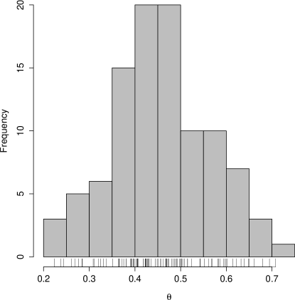
Figure 1: Histogram of the extremal index estimations from the 100 simulated Markov Chains of length 2000.

From equation (10), the extremal index $\theta$ must be known to obtain quantile estimates. The methodology applied in this study is similar to the one suggested by Fawcett and Walshaw [2006]. Once the Markovian model is fitted, 100 Markov chains of length 2000 were generated. For each chain, the extremal index is estimated using the estimator proposed by Ferro and Segers [2003] to avoid issues related to the choice of declustering parameter. In particular, the extremal index $\theta$ is estimated using the following equations:

$$\hat{\theta}(u)=\begin{cases}\max\left(1,\frac{2\left[\sum_{i=1}^{N-1}\left(T_{i}-1\right)\right]^{2}}{\left(N-1\right)\sum_{i=1}^{N-1}T_{i}^{2}}\right),&\text{if }\max\left\{T_{i}:1\leq i\leq N-1\right\}\leq 2\\ \max\left(1,\frac{2\left(\sum_{i=1}^{N-1}T_{i}\right)^{2}}{\left(N-1\right)\sum_{i=1}^{N-1}\left(T_{i}-1\right)\left(T_{i}-2\right)}\right),&\text{otherwise}\end{cases}$$ (12)

where $N$ is the number of observations exceeding the threshold $u$, $T_{i}$ is the inter-exceedance time, e.g. $T_{i}=S_{i+1}-S_{i}$ and the $S_{i}$ is the $i$-th exceedance time.

Lastly, the extremal index related to a fitted Markov chain model is estimated using the sample mean of the 100 extremal index estimations. Figure 1 represents the histogram of these 100 extremal index estimations. In this study, as lots of time series are involved, the number and length of the simulated Markov chains may be too small to lead to the most accurate extremal index estimations; but avoid intractable CPU times. If less sites are considered, it is preferable to increase these two values.

A preliminary study (not shown here) demonstrates that, for quantile estimation, this procedure was more accurate than estimating $\theta$ using the estimator of [Leadbetter, 1983]. This confirms the conclusions drawn by Fawcett [2005] for the extreme wind speed data.

3 Extreme Value Dependence Structure Assessment

Prior to performing any estimations, it is necessary to test whether: (a) the first order Markov chain assumption and (b) the extreme value dependence structure (equation (3)) are appropriate to model successive observations above the threshold $u$.

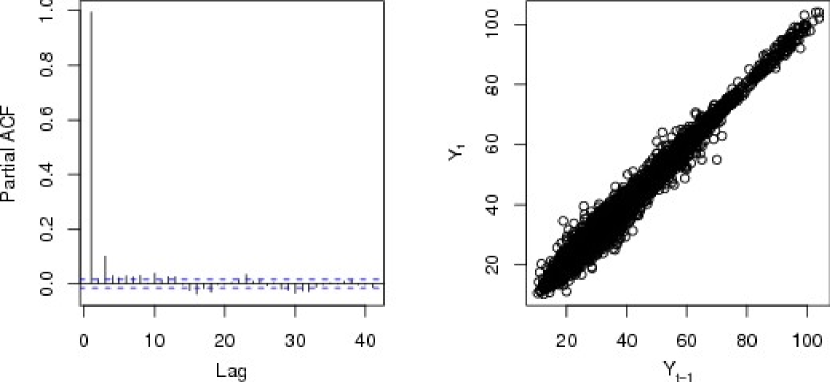
Figure 2: Autocorrelation plot (left panel) and scatterplot of the time series at lag 1 (right panel) for the Somme river at Abbeville (E6470910).

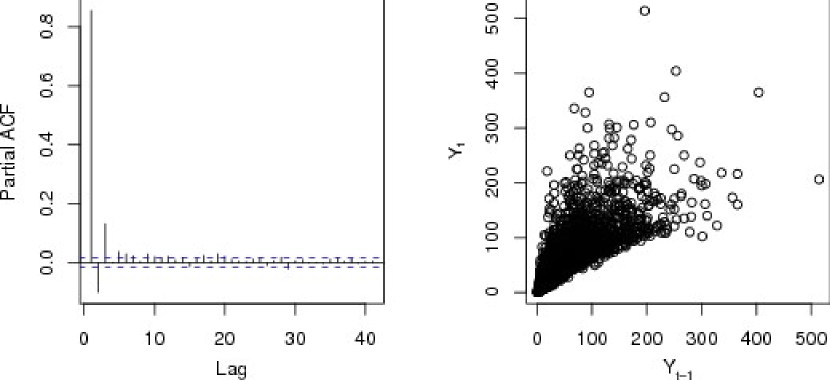
Figure 3: Autocorrelation plot (left panel) and scatterplot of the time series at lag 1 (right panel) for the Moselle river at Noirgueux (A4200630).

Figures 2 and 3 plot the auto-correlation functions and the scatter plots between two consecutive observations for two different gaging stations. As the partial autocorrelation coefficient at lag 1 is large, Figure 2 and 3 (left panels) corroborate the (a) hypothesis. However, as some partial auto-correlation coefficients are significant beyond lag 1, it may suggest that a higher-order model may be more appropriate but does not necessarily mean that a first-order assumption is completely flawed. Simplex plots [Coles and Tawn, 1991] (not shown) can be used to assess the suitability of a second-order assumption over a first-order one. For our application, it seems that a first-order model seems to be valid - except for the five slowest dynamic catchments.

Though it is an important stage because of its consequences on quantile estimates [Ledford and Tawn, 1996; Bortot and Coles, 2000], verifying the (b) hypothesis is a considerable task. An overwhelming dependence between consecutive observations at finite levels is not sufficient as it does not give any information about the dependence relation at asymptotic levels. For instance, the overwhelming dependence at lag 1 (Figure 2 and 3, right panels) does certainly not justify the use of an asymptotic dependent model.

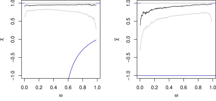
Figure 4: Plot of the $\chi$ and $\overline{\chi}$ statistics and the related 95% confidence intervals for the Somme river at Abbeville (E6470910). The solid blue lines are the theoretical bounds.

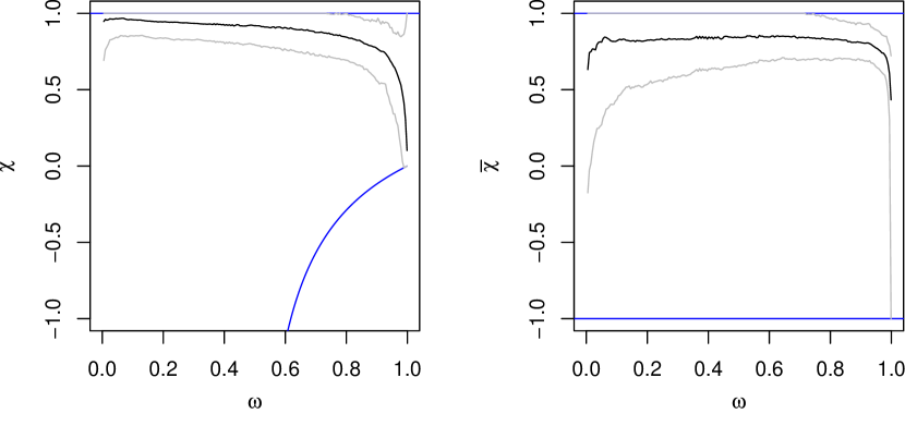
Figure 5: Plot of the $\chi$ and $\overline{\chi}$ statistics and the related 95% intervals for the Moselle river at Noirgueux (A4200630). The solid blue lines are the theoretical bounds.

Figures 4 and 5 plot the evolution of the $\chi(\omega)$ and $\overline{\chi}(\omega)$ statistics as $\omega$ increases for two different sites. For these figures, the confidence intervals are derived by bootstrapping contiguous blocks to take into account the successive observations dependence [Ledford and Tawn, 2003]. The $\chi(\omega)$ and $\overline{\chi}(\omega)$ statistics seem to depict two different asymptotic extremal dependence. From Figure 4, it seems that $\lim\chi(\omega)\gg 0$ and $\lim\overline{\chi}(\omega)=1$ for $\omega\rightarrow 1$. On the contrary, Figure 5 advocates for $\lim\chi(\omega)=0$ and $\lim\overline{\chi}(\omega)<1$ for $\omega\rightarrow 1$. Consequently, Figure 4 seems to conclude for an asymptotic dependent case while Figure 5 for an asymptotic independent case.

In theory, asymptotic (in)dependence should not be assessed using scatterplots. However, these two different features can be deduced from Figures 2 and 3. For Figure 2, the scatterplot $(Y_{t-1},Y_{t})$ is increasingly less spread as the observations becomes larger; while increasingly more spread for Figure 3. In other words, for the first case, the dependence seems to become stronger at larger levels while this is the contrary for the second case.

Table 1: $\chi(\omega)$ statistics for all stations. $\omega=0.98,0.985,0.99$.

Stations	$\omega=0.98$			$\omega=0.985$			$\omega=0.99$
	$\chi(\omega)$	95% C.I.		$\chi(\omega)$	95% C.I.		$\chi(\omega)$	95% C.I.
A3472010	0.67	(-0.02, 1.00)		0.60	(-0.02, 1.00)		0.57	(-0.01, 1.00)
A4200630	0.53	( 0.21, 0.81)		0.45	( 0.07, 0.77)		0.38	(-0.01, 0.76)
A4250640	0.55	( 0.27, 0.82)		0.49	( 0.18, 0.76)		0.41	( 0.02, 0.71)
A5431010	0.44	(-0.02, 1.00)		0.44	(-0.02, 1.00)		0.41	(-0.01, 1.00)
A5730610	0.59	( 0.25, 0.94)		0.56	( 0.20, 0.90)		0.50	( 0.07, 0.97)
A6941010	0.62	( 0.22, 0.99)		0.60	( 0.16, 1.00)		0.56	( 0.06, 1.00)
A6941015	0.63	( 0.29, 0.95)		0.60	( 0.20, 0.96)		0.58	( 0.17, 0.98)
D0137010	0.39	( 0.04, 0.69)		0.33	(-0.02, 0.67)		0.28	(-0.01, 0.69)
D0156510	0.59	( 0.25, 0.88)		0.55	( 0.20, 0.86)		0.53	( 0.14, 0.92)
E1727510	0.62	( 0.18, 0.91)		0.59	( 0.16, 0.93)		0.47	(-0.01, 0.89)
E1766010	0.63	( 0.23, 0.98)		0.59	( 0.17, 0.96)		0.54	( 0.09, 0.96)
E3511220	0.59	( 0.10, 1.00)		0.53	(-0.02, 1.00)		0.50	(-0.01, 0.99)
E4035710	0.77	( 0.02, 1.00)		0.68	(-0.02, 1.00)		0.60	(-0.01, 1.00)
E5400310	0.88	( 0.30, 1.00)		0.89	( 0.29, 1.00)		0.83	( 0.13, 1.00)
E5505720	0.91	( 0.24, 1.00)		0.87	( 0.09, 1.00)		0.86	( 0.02, 1.00)
E6470910	0.96	( 0.40, 1.00)		0.94	( 0.25, 1.00)		0.98	( 0.00, 1.00)
H0400010	0.84	( 0.12, 1.00)		0.83	( 0.02, 1.00)		0.78	(-0.01, 1.00)
H1501010	0.82	( 0.36, 1.00)		0.90	( 0.39, 1.00)		0.84	( 0.26, 1.00)
H2342010	0.68	( 0.31, 1.00)		0.67	( 0.25, 1.00)		0.60	( 0.11, 1.00)
H5071010	0.75	( 0.30, 1.00)		0.76	( 0.22, 1.00)		0.75	( 0.15, 1.00)
H5172010	0.80	( 0.47, 1.00)		0.77	( 0.42, 1.00)		0.73	( 0.30, 1.00)
H6201010	0.69	( 0.29, 1.00)		0.69	( 0.14, 1.00)		0.69	( 0.08, 1.00)
H7401010	0.85	( 0.46, 1.00)		0.85	( 0.38, 1.00)		0.81	( 0.27, 1.00)
I9221010	0.67	( 0.23, 1.00)		0.66	( 0.19, 1.00)		0.59	( 0.04, 1.00)
J0621610	0.61	( 0.25, 0.92)		0.58	( 0.20, 0.94)		0.51	( 0.08, 0.91)
K0433010	0.59	( 0.22, 0.91)		0.54	( 0.15, 0.89)		0.45	( 0.00, 0.85)
K0454010	0.71	( 0.37, 1.00)		0.67	( 0.24, 1.00)		0.65	( 0.14, 1.00)
K0523010	0.62	(-0.02, 1.00)		0.58	(-0.02, 1.00)		0.53	(-0.01, 1.00)
K0550010	0.61	( 0.22, 0.94)		0.57	( 0.15, 0.94)		0.54	( 0.07, 1.00)
K0673310	0.67	( 0.24, 1.00)		0.65	( 0.18, 1.00)		0.66	( 0.07, 1.00)
K0910010	0.65	(-0.02, 1.00)		0.61	(-0.02, 1.00)		0.58	(-0.01, 1.00)
K1391810	0.68	( 0.27, 1.00)		0.64	( 0.16, 0.98)		0.60	( 0.06, 0.96)
K1503010	0.69	( 0.38, 0.98)		0.67	( 0.30, 0.98)		0.64	( 0.23, 1.00)
K2330810	0.68	( 0.29, 1.00)		0.66	( 0.22, 1.00)		0.62	( 0.09, 1.00)
K2363010	0.65	( 0.26, 0.98)		0.66	( 0.16, 1.00)		0.61	( 0.01, 1.00)
K2514010	0.61	( 0.24, 1.00)		0.61	( 0.21, 1.00)		0.58	( 0.12, 1.00)
K2523010	0.53	(-0.02, 1.00)		0.53	(-0.02, 1.00)		0.51	(-0.01, 1.00)
K2654010	0.68	( 0.37, 1.00)		0.68	( 0.31, 1.00)		0.60	( 0.10, 1.00)
K2674010	0.60	( 0.25, 0.89)		0.58	( 0.22, 0.94)		0.54	( 0.08, 0.95)
K2871910	0.62	( 0.26, 0.95)		0.57	( 0.15, 0.94)		0.56	( 0.10, 0.97)
K2884010	0.62	( 0.25, 1.00)		0.57	( 0.17, 0.97)		0.59	( 0.16, 1.00)
K3222010	0.56	( 0.21, 0.90)		0.53	( 0.18, 0.93)		0.46	( 0.11, 0.89)
K3292020	0.59	( 0.27, 0.91)		0.57	( 0.17, 0.91)		0.48	( 0.07, 0.90)
K4470010	0.76	( 0.39, 1.00)		0.77	( 0.40, 1.00)		0.73	( 0.27, 1.00)
K5090910	0.64	( 0.27, 0.93)		0.64	( 0.26, 0.96)		0.58	( 0.12, 0.98)
K5183010	0.57	( 0.14, 0.91)		0.56	( 0.15, 0.96)		0.53	( 0.06, 0.97)
K5200910	0.63	( 0.24, 0.93)		0.62	( 0.20, 0.95)		0.56	( 0.11, 0.97)
L0140610	0.73	( 0.23, 1.00)		0.66	( 0.15, 1.00)		0.58	(-0.01, 1.00)
L0231510	0.59	( 0.16, 0.91)		0.55	( 0.11, 0.92)		0.53	(-0.01, 0.92)
L0400610	0.74	(-0.02, 1.00)		0.65	(-0.02, 1.00)		0.61	(-0.01, 1.00)

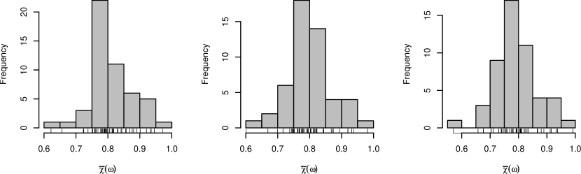
Figure 6: Histograms of the $\overline{\chi}(\omega)$ statistics for different $\omega$ values. Left panel: $\omega=0.98$, middle panel: $\omega=0.985$ and right panel: $\omega=0.99$.

Two specific cases for different asymptotic dependence structures were illustrated. Table 1 shows the evolution of the $\chi(\omega)$ statistics as $\omega$ increases for all the sites under study. Most of the stations have significantly positive $\chi(\omega)$ values. In addition, only 13 sites have a 95% confidence interval that contains the 0 value. For 9 of these stations, the 95% confidence intervals correspond to the theoretical lower and upper bounds; so that uncertainties are too large to determine the extremal dependence class. For the $\overline{\chi}$ statistic, results are less clear-cut. Figure 6 represents the histograms for $\overline{\chi}(\omega)$ for successive $\omega$ values. Despite only a few observations being close to 1, most of the stations have a $\overline{\chi}(\omega)$ value greater than 0.75. These values can be considered as significantly high as $-1<\overline{\chi}(\omega)\leq 1$, for all $\omega$. Consequently, models of the form (1)–(3) may be suited to model the extremal dependence between successive observations.

Other methods exist to test the extremal dependence but were unconvincing for our application [Ledford and Tawn, 2003; Falk and Michel, 2006]. Indeed, the approach of Falk and Michel [2006] does not take into account the dependence between $Y_{t-1}$ and $Y_{t}$; while the test of Ledford and Tawn [2003] appears to be poorly discriminatory for our case study.

4 Performance of the Markovian Models on Quantile Estimation

4.1 Comparison between Markovian estimators

In this section, the performance of six different extremal dependence structures is analyzed on the 50 gaging stations introduced in section 1. These models are: $log$ for the logistic, $nlog$ for the negative logistic, $mix$ for the mixed models and their relative asymmetric counterparts - e.g. $alog$, $anlog$ and $amix$. To assess the impact of the dependence structure on flood peak estimation, the efficiency of each model to estimate quantiles with return periods 2, 10, 20, 50 and 100 years is evaluated.

As practitioners often have to deal with small record lengths in practice, the performance of the Markovian models is analyzed on all sub time series of length 5, 10, 15 and 20 years. Finally, to assess the efficiency for all the gaging stations considered in this study, the normalized bias ($\mathbf{nbias}$), the variance ($\mathbf{var}$) and the normalized mean squared error ($\mathbf{nmse}$) are computed:

$$nbias = \frac{1}{N}\sum_{i=1}^{N}\frac{\hat{Q}_{i,T}-Q_{T}}{Q_{T}}$$ (13)

$$var = \frac{1}{N-1}\sum_{i=1}^{N}\left(\frac{\hat{Q}_{i,T}-Q_{T}}{Q_{T}}-nbias\right)^{2}$$ (14)

$$nmse = \frac{1}{N}\sum_{i=1}^{N}\left(\frac{\hat{Q}_{i,T}-Q_{T}}{Q_{T}}\right)^{2}$$ (15)

where $Q_{T}$ is the benchmark $T$-year return level and $\hat{Q}_{i,T}$ is the $i$-th estimate of $Q_{T}$.

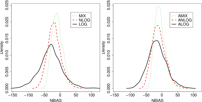
Figure 7: Densities of the normalized biases of $Q_{20}$ estimates for the symmetric Markovian models (left panel) and the asymmetric ones (right panel). Target site record length: 5 years.

Figure 7 depicts the $nbias$ densities for $Q_{20}$ with a record length of 5 years. It is overwhelming that the extremal dependence structure has a great impact on the estimation of $Q_{20}$. Comparing the two panels, it can be noticed that the symmetric dependence structures give spreader densities; that is, more variable estimates. Independently of the symmetry, Figure 7 shows that the mixed dependence family is more accurate.

Table 2: Several characteristics of the Markovian estimators on $Q_{50}$ estimation as the record length increases. Standard errors are reported in brackets.

Model	5 years				10 years				15 years				20 years
	$nbias$	$var$	$nmse$		$nbias$	$var$	$nmse$		$nbias$	$var$	$nmse$		$nbias$	$var$	$nmse$
$log$	-0.35	0.54	0.66		-0.32	0.32	0.42		-0.30	0.23	0.32		-0.28	0.17	0.25
	(16e-3)	(22e-3)	(18e-3)		(12e-3)	(12e-3)	(14e-3)		(11e-3)	(9e-3)	(12e-3)		(9e-3)	(7e-3)	(11e-3)
$nlog$	-0.21	0.20	0.24		-0.20	0.11	0.15		-0.18	0.08	0.12		-0.18	0.06	0.09
	(10e-3)	(7e-3)	(11e-3)		(7e-3)	(4e-3)	(9e-3)		(6e-3)	(3e-3)	(8e-3)		(5e-3)	(2e-3)	(7e-3)
$mix$	-0.08	0.14	0.14		-0.07	0.08	0.08		-0.06	0.05	0.06		-0.05	0.04	0.04
	(8e-3)	(5e-3)	(8e-3)		(6e-3)	(2e-3)	(6e-3)		(5e-3)	(2e-3)	(5e-3)		(4e-3)	(1e-3)	(5e-3)
$alog$	-0.15	0.39	0.41		-0.13	0.22	0.24		-0.11	0.16	0.17		-0.10	0.12	0.13
	(14e-3)	(15e-3)	(14e-3)		(10e-3)	(9e-3)	(11e-3)		(9e-3)	(6e-3)	(9e-3)		(8e-3)	(4e-3)	(8e-3)
$anlog$	-0.10	0.20	0.21		-0.09	0.11	0.12		-0.08	0.08	0.09		-0.08	0.06	0.06
	(10e-3)	(7e-3)	(10e-3)		(7e-3)	(4e-3)	(8e-3)		(6e-3)	(2e-3)	(6e-3)		(5e-3)	(2e-3)	(6e-3)
$amix$	-0.06	0.11	0.12		-0.05	0.06	0.06		-0.04	0.04	0.05		-0.03	0.03	0.03
	(7e-3)	(4e-3)	(7e-3)		(6e-3)	(2e-3)	(6e-3)		(5e-3)	(1e-3)	(5e-3)		(4e-3)	(1e-3)	(4e-3)

Table 2 shows the $nbias$, $var$ and $nmse$ statistics for all the Markovian estimators as the record length increases for quantile $Q_{50}$. This table confirms results derived from Figure 7. Indeed, the asymmetric dependence structures give less variable and biased estimates - as their $nbias$ and $var$ statistics are smaller. In addition, whatever the record length is, the Markovian models perform with the same hierarchy; that is the $mix$ and $amix$ models are by far the most accurate estimators - i.e. with the smallest $nmse$ values. The same results (not shown) have been found for other quantiles.

From an hydrological point of view, these two results are not surprising. The symmetric models suppose that the variables $Y_{t}$ and $Y_{t+1}$ are exchangeable. In our context, exchangeability means that the time series are reversible - e.g. the time vector direction has no importance. When dealing with AM or POT and stationary time series, it is a reasonable hypothesis. For example, the MLE remains the same with any permutations of the AM/POT sample. However, when modeling all exceedances, the time direction can not be considered as reversible as flood hydrographs are clearly non symmetric.

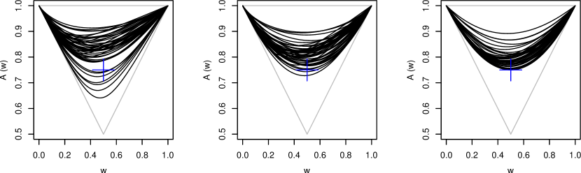
Figure 8: Representation of the Pickands’ dependence functions for the 50 gaging stations. Left panel : $alog$, middle panel: $anlog$ and right panel: $amix$. “+” represents the theoretical dependence bound for the $amix$ model.

The Pickands’ dependence function $A(\omega)$ [Pickands, 1981] is another representation for the extremal dependence structure for any extreme value distribution. $A(\omega)$ is related to the $V$ function in equation (3) as follows:

$$A(\omega)=\frac{V(z_{1},z_{2})}{z_{1}^{-1}+z_{2}^{-1}},\qquad\omega=\frac{z_{1}}{z_{1}+z_{2}}$$ (16)

Figure 8 represents the Pickands’ dependence function for all the gaging stations and the three asymmetric Markovian models. One major specificity of the mixed models is that these models can not account for perfect dependence cases. In particular, the Pickands’ dependence functions for the mixed models satisfy $A(0.5)\geq 0.75$ while $A(0.5)\in[0.5,1]$ for the logistic and negative logistic models. From Figure 8, it can be seen that only few stations have a dependence function that could not be modeled by the $amix$ model. Therefore, the dependence range limitation of the $amix$ model does not seem too restrictive.

In this section, the effect of the extremal dependence structure has been assessed. It has been established that the symmetric models are hydrologically inconsistent as they could not reproduce the flood event asymmetry. In addition, for all the quantiles analyzed, the asymmetric mixed model is the most accurate for flood peak estimations. Therefore, in the remainder of this section, only the $amix$ model will be compared to conventional POT estimators.

4.2 Comparison between $amix$ and conventional POT estimators

In this section, the performance of the $amix$ estimator is compared to the estimators usually used in flood frequency analysis. For this purpose, the quantile estimates derived from the Maximum Likelihood Estimator ($\mathbf{MLE}$), the Unbiased and Biased Probability Weighted moments estimators [Hosking and Wallis, 1987] ($\mathbf{PWU}$ and $\mathbf{PWB}$ respectively) are considered.

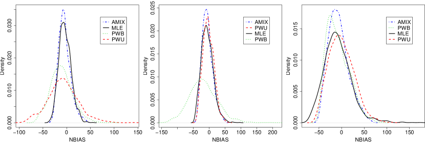
Figure 9: Densities of the normalized biases for the $amix$ model and the $MLE$, $PWU$, and $PWB$ estimators for quantiles $Q_{5}$ (left panel), $Q_{10}$ (middle panel) and $Q_{20}$ (right panel). Record length: 5 years.

Figure 9 depicts the $nbias$ densities for the $amix$, $MLE$, $PWU$ and $PWB$ estimators related to the $Q_{5}$, $Q_{10}$ and $Q_{20}$ estimations with a record length of 5 years. It can be seen that $amix$ is the most accurate model for all quantiles. Indeed, the $amix$ $nbias$ densities are the most sharp with a mode close to 0. Focusing only on “classical” estimators (e.g. $MLE$, $PWU$ and $PWB$), there is no estimator that perform better than any other anytime. These two results advocate the use of the $amix$ model.

Table 3: Several characteristics of the $amix$, $MLE$, $PWU$ and $PWB$ estimators for $Q_{50}$ estimation as the record length increases. Standard errors are reported in brackets.

Model	5 years				10 years				15 years				20 years
	$nbias$	$var$	$nmse$		$nbias$	$var$	$nmse$		$nbias$	$var$	$nmse$		$nbias$	$var$	$nmse$
$amix$	-0.06	0.11	0.12		-0.05	0.06	0.07		-0.04	0.04	0.05		-0.04	0.03	0.03
	(8e-3)	(4e-3)	(8e-3)		(6e-3)	(2e-3)	(6e-3)		(5e-3)	(1e-3)	(5e-3)		(4e-3)	(1e-3)	(4e-3)
$MLE$	-0.13	0.25	0.27		-0.14	0.13	0.14		-0.13	0.08	0.10		-0.11	0.05	0.07
	(12e-3)	(15e-3)	(12e-3)		(8e-3)	(6e-3)	(9e-3)		(7e-3)	(3e-3)	(7e-3)		(5e-3)	(2e-3)	(6e-3)
$PWU$	0.08	0.30	0.31		-0.01	0.15	0.15		-0.03	0.10	0.10		-0.03	0.06	0.06
	(13e-3)	(13e-3)	(13e-3)		(9e-3)	(6e-3)	(9e-3)		(7e-3)	(3e-3)	(7e-3)		(6e-3)	(2e-3)	(6e-3)
$PWB$	-0.07	0.20	0.21		-0.10	0.11	0.12		-0.11	0.08	0.09		-0.10	0.05	0.06
	(10e-3)	(8e-3)	(11e-3)		(7e-3)	(4e-3)	(8e-3)		(6e-3)	(2e-3)	(7e-3)		(5e-3)	(1e-3)	(6e-3)

Table 3 shows the performance of each estimator to estimate $Q_{50}$ as the record length increases. It can be seen that the $amix$ model performs better than the conventional estimators for the whole range of record lengths analyzed. First, $amix$ has the same bias than the conventional estimators. Thus, the $amix$ dependence structure seems to be suited to estimate flood quantile estimates. Second, because of its smaller variance, $amix$ is more accurate than $MLE$, $PWU$ and $PWB$ estimators. This smaller variance is mainly a result of all of the exceedances (not only cluster maxima) being used in the inference procedure. Consequently, the $amix$ model has a smaller $nmse$ - around half of the conventional models ones.

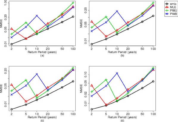
Figure 10: Evolution of the $nmse$ as the return period increases for the $amix$, $MLE$, $PWU$ and $PWB$ estimators. Record length: (a) 5 years, (b) 10 years, (c) 15 years and (d) 20 years.

Figure 10 shows the evolution of the $nmse$ as the return period increases for the $amix$, $MLE$, $PWU$ and $PWB$ models. This figure corroborates the conclusions drawn from Figure 9 and Table 3. It can be seen that the $amix$ model has the smallest $nmse$, independently of the return period and the record length. In addition, the $amix$ becomes increasingly more efficient as the return period increases - mostly for return periods greater than 20 years. While the conventional estimators present an erratic $nmse$ behavior as the return period increases, the $amix$ model is the only one that has a smooth evolution. To conclude, these results confirm that the $amix$ model clearly improves flood peak quantile estimates - especially for large return periods.

5 Inference on Other Flood Characteristics

As all exceedances are modeled using a first order Markov chain, it is possible to infer other quantities than flood peaks - e.g. volume and duration. In this section, the ability of these Markovian models to reproduce the flood duration is analyzed. For this purpose, the most severe flood hydrographs within each year are considered and normalized by their peak values. Consequently, from this observed normalized hydrograph set, two flood characteristics derived from a data set of hydrographs [Robson and Reed, 1999; Sauquet et al., 2008] are considered: (a) the duration $d_{mean}$ above 0.5 of the normalized hydrograph set mean and (b) the median $d_{med}$ of the durations above 0.5 of each normalized hydrograph.

5.1 Global Performance

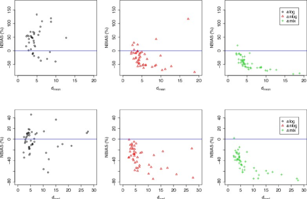
Figure 11: $d_{mean}$ and $d_{med}$ normalized biases in function of the theoretical values for the three asymmetric Markovian models.

Figure 11 plots the flood durations $d_{mean}$ and $d_{med}$ biases derived from the three asymmetric Markovian models in function of their empirical estimates. It can be seen that no model leads to accurate flood duration estimations. In addition, the extremal dependence structure has a clear impact on these estimations. In particular, the $anlog$ and $amix$ models seem to underestimate the flood durations, while the $alog$ model leads to overestimations. Consequently, two different conclusions can be drawn. First, as large durations are poorly estimated, higher order Markov chains may be of interest. However, this is a considerable task as higher dimensional multivariate extreme value distributions often lead to numerical problems. Instead of considering higher order, another alternative may be to change daily observations for $d$-day observations - where $d$ is larger than 1. Second, it is overwhelming that the extremal dependence structure affects the flood duration estimations. As noticed in Section 2.1, there is no finite parametrization for the extremal dependence structure $V$ - see Equation (3). Consequently, it seems reasonable to suppose that one suited for flood hydrograph estimation may exist.

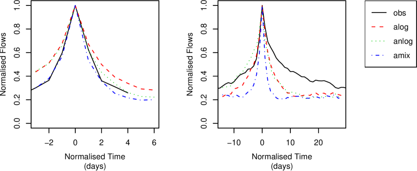
Figure 12: Observed and simulated normalized mean hydrographs for the J0621610 (left panel) and the L0400610 (right panel) stations.

Figure 12 depicts the observed normalized mean hydrographs and the ones predicted by the three asymmetric Markovian models. For the J0621610 station (left panel), the normalized hydrograph is well estimated by the three models; whereas for the L0400610 station (right panel), the normalized hydrograph is poorly predicted. This result confirms the inability of the three Markovian models to reproduce long flood events with daily data and a first order Markov chain.

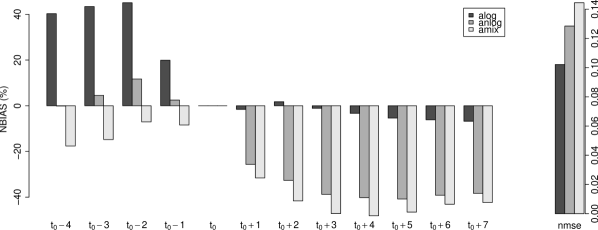
Figure 13: Evolution of the biases for the normalized mean hydrograph estimations in function of the distance of the flood peak time.

Figure 13 represents the biases related to each value of the normalized mean hydrograph. In addition, to help estimator comparison, the $nmse$ is reported at the right side. It can be seen that the $alog$ model dramatically overestimates the hydrograph rising limb while giving reasonable estimations for the falling phase. The $anlog$ model slightly overestimates the rising part while strongly underestimates the falling one. The $amix$ model always leads to underestimations - this is more pronounced for the falling limb. However, despite these different behaviors, these three estimators seems to have a similar performance - in terms of $nmse$.

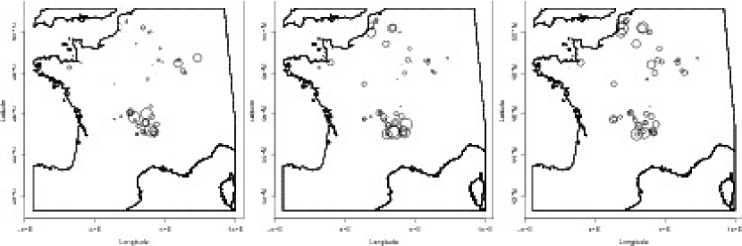
Figure 14: $nmse$ spatial distribution according for the three Markovian models. Left panel: $alog$, middle panel: $anlog$ and right panel: $amix$. The radius is proportional to the $nmse$ value.

Figure 14 represents the spatial distribution of the $nmse$ on the normalized mean hydrograph estimation for each Markovian model. It seems that there is a specific spatial distribution. In particular, the worst cases are related to the middle part of France. In addition, for different extremal dependence structures, the best $nmse$ values correspond to different spatial locations. The $alog$ model is more accurate for the extreme north part of France; the $anlog$ model is more efficient for the east part of France; while the $amix$ model performs best in the middle part of France. Consequently, as at a global scale no model is accurate to estimate the normalized mean hydrograph, it is worth trying to identify which catchment types are related to the best estimations.

For our data set, this is a considerable task. No standard statistical technique lead to reasonable results. In particular, the principal component analysis, hierarchical classification, sliced inverse regression lead to no conclusion about which catchment types are more suitable for our models. Only a regression approach gives some first guidelines. For this purpose, a regression between the $nbias$ on the $d_{mean}$ estimation for each asymmetric model and some geomorphologic and hydrologic indices are performed. The effect of the drainage area, an index of catchment slope derived from the hypsometric curve [Roche, 1963], the Base Flow Index ($\mathbf{BFI}$) [Tallaksen and Van Lanen, 2004, Section 5.3.3] and an index characterizing the rainfall persistence [Vaskova and Francès, 1998] are considered.

$$nbias\left(d_{mean};anlog\right) = 0.89-2.19BFI,\qquad R^{2}=0.40$$ (17)

$$nbias\left(d_{mean};amix\right) = 0.49-1.74BFI,\qquad R^{2}=0.43$$ (18)

From equations (17) and (18), the $BFI$ variable explains around 40% of the variance. Despite the fact that a large variance proportion is not taken into account, the $BFI$ is clearly related to the $d_{mean}$ estimation performance. These equations indicate that the $anlog$ (resp. $amix$) model is more accurate to reproduce the $d_{mean}$ variable for gaging stations with a $BFI$ around 0.4 (resp. 0.28). These $BFI$ values correspond to catchments with moderate up to flash flow regimes respectively. These results corroborate the ones derived from Figure 13: the first order Markovian models with a 1-day lag conditioning are not appropriate for long flood duration estimations. Consequently, while no physiographic characteristic is related to the $alog$ performance; it is suggested, for such 1-day lag conditioning, to use the $anlog$ and $amix$ models for quick basins.

6 Conclusion

Despite that univariate EVT is widely applied in environmental sciences, its multivariate extension is rarely considered. This work tries to promote the use of the MEVT in hydrology. In this work, the bivariate case was considered as the dependence between two successive observations was modeled using a first order Markov chain. This approach has two main advantages for practitioners as: (a) the number of data to be inferred increases considerably and (b) other features can be estimated - flood duration, volume.

In this study, a comparison between six different extremal dependence structures (including both symmetric and asymmetric forms) has been performed. Results show that an asymmetric dependence structure is more relevant. From a hydrological point of view, this asymmetry is rational as flood hydrographs are asymmetric. In particular, for our data, the asymmetric mixed model gives the most accurate flood peak estimations and clearly improves flood peak estimations compared to conventional estimators independently of the return period considered.

The ability of these Markovian models to estimate the flood duration was carried out. It has been shown that, at first sight, no dependence structure is able to reproduce the flood hydrograph accurately. However, it seems that the $anlog$ and $amix$ models may be more appropriate when dealing with moderate up to flash flow regimes. These results depend strongly on the conditioning term (i.e. $\Pr[Y_{t}\leq y_{t}|Y_{t-\delta}=y_{t-\delta}]$) of the first order Markov chain and on the auto-correlation within the time series. In our application, $\delta=1$ and daily time step was considered.

More general conclusions can be drawn. The weakness of the proposed models to derive consistent flood hydrographs may not be related to the daily time step but to the inadequacy between the conditioning term and the flood dynamics. To ensure better results, higher order Markov chains may be of interest [Fawcett and Walshaw, 2006]. However, as numerical problems may arise, another alternative may be to still consider a first order chain but to change the “conditioning lag value” $\delta$. In particular, for some basins, it may be more relevant to condition the Markov chain with a larger but more appropriate lag value.

Another option to improve the proposed models for flood hydrograph estimation is to use a more suitable dependence function $V$. As there is no finite parametrization for the extremal dependence structure, it seems reasonable that one more appropriate for flood hydrographs may exist. In this work, results show that the $anlog$ model is more able to reproduce the hydrograph rising part, while the $alog$ is better for the falling phase. Define

$$V\left(z_{1},z_{2}\right)=\alpha V_{1}\left(z_{1},z_{2}\right)+\beta V_{2}\left(z_{1},z_{2}\right)$$

where $V_{1}$ (resp. $V_{2}$) is the extremal dependence function for the $alog$ (resp. $anlog$) model and $\alpha$ and $\beta$ are real constants such as $\alpha+\beta=1$. By definition, $V$ is a new extremal dependence function. In particular, $V$ may combine the accuracy of the $alog$ and $anlog$ models for both the rising and falling part of the flood hydrograph. Another alternative may be to look at non-parametric Pickands’ dependence function estimators [Capéraà et al., 1997] but that will require techniques to simulate Markov chains from these non-parametric estimations.

All statistical analysis were performed within the R Development Core Team [2007] framework. In particular, the POT package [Ribatet, 2007] integrates the tools that were developed to carry out the modeling effort presented in this paper. This package is available, free of charge, at the website http://www.R-project.org, section CRAN, Packages or at its own webpage http://pot.r-forge.r-project.org/.

Appendix A Parametrization for the Extremal Dependence

This annex presents some useful results for the six extremal dependence models that have been considered in this work. As first order Markov chains were used, only the bivariate results are described.

Table 4: Partial and mixed partial derivatives, definition domain, total independent and perfect dependent cases for each extremal symmetric dependence function $V$.

Model	Symmetric Models
	$log$	$nlog$	$mix$
$V(x,y)$	$\left(x^{-1/\alpha}+y^{-1/\alpha}\right)^{\alpha}$	$\frac{1}{x}+\frac{1}{y}-\left(x^{\alpha}+y^{\alpha}\right)^{-1/\alpha}$	$\frac{1}{x}+\frac{1}{y}-\frac{\alpha}{x+y}$
$V_{1}(x,y)$	$-x^{-\frac{1}{\alpha}-1}V(x,y)^{\frac{\alpha-1}{\alpha}}$	$-\frac{1}{x^{2}}+x^{\alpha-1}\left(x^{\alpha}+y^{\alpha}\right)^{-\frac{1}{\alpha}-1}$	$-\frac{1}{x^{2}}+\frac{\alpha}{\left(x+y\right)^{2}}$
$V_{2}(x,y)$	$-y^{-\frac{1}{\alpha}-1}V(x,y)^{\frac{\alpha-1}{\alpha}}$	$-\frac{1}{y^{2}}+y^{\alpha-1}\left(x^{\alpha}+y^{\alpha}\right)^{-\frac{1}{\alpha}-1}$	$-\frac{1}{y^{2}}+\frac{\alpha}{\left(x+y\right)^{2}}$
$V_{12}(x,y)$	$-(xy)^{-\frac{1}{\alpha}-1}\frac{1-\alpha}{\alpha}V(x,y)^{\frac{\alpha-2}{\alpha}}$	$-(\alpha+1)(xy)^{\alpha-1}\left(x^{\alpha}+y^{\alpha}\right)^{-\frac{1}{\alpha}-2}$	$-\frac{2\alpha}{\left(x+y\right)^{3}}$
$A(w)$	$\left[(1-w)^{\frac{1}{\alpha}}+w^{\frac{1}{\alpha}}\right]^{\alpha}$	$1-\left[(1-w)^{-\alpha}+w^{-\alpha}\right]^{-\frac{1}{\alpha}}$	$1-w\left(1-w\right)\alpha$
Independence	$\alpha=1$	$\alpha\rightarrow 0$	$\alpha=0$
Total dependence	$\alpha\rightarrow 0$	$\alpha\rightarrow+\infty$	Never reached
Constraint	$0<\alpha\leq 1$	$\alpha>0$	$0\leq\alpha\leq 1$

Table 5: Partial and mixed partial derivatives, definition domain, total independent and perfect dependent cases for each extremal asymmetric dependence function $V$.

Model	Asymmetric Models
	$alog$	$anlog$	$amix$
$V(x,y)$	$\frac{1-\theta_{1}}{x}+\frac{1-\theta_{2}}{y}+\left[\left(\frac{x}{\theta_{1}}\right)^{-1/\alpha}+\left(\frac{y}{\theta_{2}}\right)^{-1/\alpha}\right]^{\alpha}$	$\frac{1}{x}+\frac{1}{y}-\left[\left(\frac{x}{\theta_{1}}\right)^{\alpha}+\left(\frac{y}{\theta_{2}}\right)^{\alpha}\right]^{-1/\alpha}$	$\frac{1}{x}+\frac{1}{y}-\frac{\left(2\alpha+\theta\right)x+\left(\alpha+\theta\right)y}{\left(x+y\right)^{2}}$
$V_{1}(x,y)$	$-\frac{1-\theta_{1}}{x^{2}}-\theta_{1}^{\frac{1}{\alpha}}x^{-\frac{1}{\alpha}-1}\left[\left(\frac{x}{\theta_{1}}\right)^{-1/\alpha}+\left(\frac{y}{\theta_{2}}\right)^{-1/\alpha}\right]^{\alpha-1}$	$-\frac{1}{x^{2}}+\theta_{1}^{-\alpha}x^{\alpha-1}\left[\left(\frac{x}{\theta_{1}}\right)^{\alpha}+\left(\frac{y}{\theta_{2}}\right)^{\alpha}\right]^{-1/\alpha-1}$	$-\frac{1}{x^{2}}-\frac{2\alpha+\theta}{(x+y)^{2}}+2\frac{(2\alpha+\theta)x+(\alpha+\theta)y}{(x+y)^{3}}$
$V_{2}(x,y)$	$-\frac{1-\theta_{2}}{y^{2}}-\theta_{2}^{\frac{1}{\alpha}}y^{-\frac{1}{\alpha}-1}\left[\left(\frac{x}{\theta_{1}}\right)^{-1/\alpha}+\left(\frac{y}{\theta_{2}}\right)^{-1/\alpha}\right]^{\alpha-1}$	$-\frac{1}{y^{2}}+\theta_{2}^{-\alpha}y^{\alpha-1}\left[\left(\frac{x}{\theta_{1}}\right)^{\alpha}+\left(\frac{y}{\theta_{2}}\right)^{\alpha}\right]^{-1/\alpha-1}$	$-\frac{1}{y^{2}}-\frac{\alpha+\theta}{(x+y)^{2}}+2\frac{(2\alpha+\theta)x+(\alpha+\theta)y}{(x+y)^{3}}$
$V_{12}(x,y)$	$\frac{\alpha-1}{\alpha}(\theta_{1}\theta_{2})^{\frac{1}{\alpha}}(xy)^{-\frac{1}{\alpha}-1}\left[\left(\frac{x}{\theta_{1}}\right)^{-1/\alpha}+\left(\frac{y}{\theta_{2}}\right)^{-1/\alpha}\right]^{\alpha-2}$	$-(\alpha+1)(\theta_{1}\theta_{2})^{-\alpha}(xy)^{\alpha-1}\left[\left(\frac{x}{\theta_{1}}\right)^{\alpha}+\left(\frac{y}{\theta_{2}}\right)^{\alpha}\right]^{-1/\alpha-2}$	$\frac{6\alpha+4\theta}{(x+y)^{3}}-6\frac{(2\alpha+\theta)x+(\alpha+\theta)y}{(x+y)^{4}}$
$A(w)$	$\left(1-\theta_{1}\right)\left(1-w\right)+\left(1-\theta_{2}\right)w+\left[(1-w)^{\frac{1}{\alpha}}\theta_{1}^{\frac{1}{\alpha}}+w^{\frac{1}{\alpha}}\theta_{2}^{\frac{1}{\alpha}}\right]^{\alpha}$	$1-\left[\left(\frac{1-w}{\theta_{1}}\right)^{-\alpha}+\left(\frac{w}{\theta_{2}}\right)^{-\alpha}\right]^{-\frac{1}{\alpha}}$	$\theta w^{3}+\alpha w^{2}-\left(\alpha+\theta\right)w+1$
Independence	$\alpha=1$ or $\theta_{1}=0$ or $\theta_{2}=0$	$\alpha\rightarrow 1$ or $\theta_{1}\rightarrow 0$ or $\theta_{2}\rightarrow=0$	$\alpha=\theta=0$
Total dependence	$\alpha\rightarrow 0$	$\alpha\rightarrow+\infty$	Never reached
Constraint	$0<\alpha\leq 1$, $0\leq\theta_{1},\theta_{2}\leq 1$	$\alpha>0$, $0<\theta_{1},\theta_{2}\leq 1$	$\alpha\geq 0$, $\alpha+2\theta\leq 1$, $\alpha+3\theta\geq 0$

References

- Bortot and Coles [2000] P. Bortot and S. Coles. The multivariate Gaussian tail model: An application to oceanographic data. Journal of the Royal Statistical Society. Series C: Applied Statistics, 49(1):31–49, 2000.
- Bortot and Tawn [1998] P. Bortot and J.A. Tawn. Models for the extremes of Markov chains. Biometrika, 85(4):851–867, 1998. ISSN 00063444.
- Capéraà et al. [1997] P. Capéraà, A.-L. Fougères, and C. Genest. A nonparametric estimation procedure for bivariate extreme value copulas. Biometrika, 84(3):567–577, 1997. ISSN 00063444.
- Coles [2001] S. Coles. An Introduction to Statistical Modelling of Extreme Values. Springer Series in Statistics. Springers Series in Statistics, London, 2001.
- Coles and Tawn [1991] S. Coles and J.A. Tawn. Modelling Extreme Multivariate Events. Journal of the Royal Statistical Society. Series B (Methodological), 53(2):377–392, 1991. ISSN 0035-9246.
- Coles et al. [1994] S. Coles, J.A. Tawn, and R.L. Smith. A seasonal Markov model for extremely low temperature. Environmetrics, 5:221–239, 1994.
- Coles et al. [1999] S. Coles, J. Heffernan, and J.A. Tawn. Dependence Measures for Extreme Value Analyses. Extremes, 2(4):339–365, December 1999.
- Cunderlik and Ouarda [2006] J.M. Cunderlik and T.B.M.J. Ouarda. Regional flood-duration-frequency modeling in the changing environment. Journal of Hydrology, 318(1-4):276–291, 2006.
- Falk and Michel [2006] M. Falk and R. Michel. Testing for tail independence in extreme value models. Annal. Inst. Stat. Math., 58(2):261–290, 2006. ISSN 00203157.
- Fawcett [2005] L. Fawcett. Statistical Methodology for the Estimation of Environmental Extremes. PhD thesis, University of Newcastle upon Tyne, 2005.
- Fawcett and Walshaw [2006] L. Fawcett and D. Walshaw. Markov chain models for extreme wind speeds. Environmetrics, 17(8):795–809, 2006. ISSN 11804009.
- Ferro and Segers [2003] C.A.T. Ferro and J. Segers. Inference for clusters of extreme values. Journal of the Royal Statistical Society. Series B: Statistical Methodology, 65(2):545–556, 2003. ISSN 13697412.
- Galambos [1975] J. Galambos. Order statistics of samples from multivariate distributions. Journal of the American Statistical Association, 9:674–680, 1975.
- Gumbel [1960] E.J. Gumbel. Bivariate exponential distributions. Journal of the American Statistical Association, 55(292):698–707, 1960.
- Hosking and Wallis [1987] J.R.M. Hosking and J.R. Wallis. Parameter and Quantile Estimation for the Generalized Pareto Distribution. Technometrics, 29(3):339–349, 1987.
- Joe [1990] H. Joe. Families of min-stable multivariate exponential and multivariate extreme value distributions. Statist. Probab. Lett., 9:75–82, 1990.
- Kjeldsen and Jones [2007] T.R. Kjeldsen and D. Jones. Estimation of an index flood using data transfer in the UK. Hydrol. Sci. J., 52(1):86–98, 2007. ISSN 02626667.
- Kjeldsen and Jones [2006] T.R. Kjeldsen and D.A. Jones. Prediction uncertainty in a median-based index flood method using L moments. Water Resources Research, 42(7):–, 2006. ISSN 00431397.
- Leadbetter [1983] M.R. Leadbetter. Extremes and local dependence in stationary sequences. Probability Theory and Related Fields (Historical Archive), 65(2):291–306, 1983.
- Ledford and Tawn [1996] A.W. Ledford and J.A. Tawn. Statistics for near independence in multivariate extreme values. Biometrika, 83:169–187, 1996.
- Ledford and Tawn [2003] A.W. Ledford and J.A. Tawn. Diagnostics for dependence within time series extremes. Journal of the Royal Statistical Society. Series B: Statistical Methodology, 65(2):521–543, 2003.
- Lindgren and Rootzen [1987] G. Lindgren and H. Rootzen. Extreme values: theory and technical applications. Scandinavian journal of statistics, 14(4):241–279, 1987.
- Pickands [1981] J. Pickands. Multivariate Extreme Value Distributions. In Proceedings 43rd Session International Statistical Institute, 1981.
- R Development Core Team [2007] R Development Core Team. R: A Language and Environment for Statistical Computing. R Foundation for Statistical Computing, Vienna, Austria, 2007. URL http://www.R-project.org. ISBN 3-900051-07-0.
- Reis Jr. and Stedinger [2005] D.S. Reis Jr. and J.R. Stedinger. Bayesian MCMC flood frequency analysis with historical information. Journal of Hydrology, 313(1-2):97–116, 2005. ISSN 00221694.
- Resnick [1987] S.I. Resnick. Extreme Values, Regular Variation and Point Processes. New–York: Springer–Verlag, 1987.
- Ribatet [2007] M. Ribatet. POT: Modelling Peaks Over a Threshold. R News, 7(1):34–36, April 2007.
- Ribatet et al. [2007a] M. Ribatet, E. Sauquet, J.-M. Grésillon, and T.B.M.J. Ouarda. A regional Bayesian POT model for flood frequency analysis. Stochastic Environmental Research and Risk Assessment (SERRA), 21(4):327–339, 2007a.
- Ribatet et al. [2007b] M. Ribatet, E. Sauquet, J.-M. Grésillon, and T.B.M.J. Ouarda. Usefulness of the Reversible Jump Markov Chain Monte Carlo Model in Regional Flood Frequency Analysis. Water Resources Research, 43(8):W08403, 2007b. doi: 10.1029/2006WR005525.
- Robson and Reed [1999] A.J. Robson and D.W. Reed. Flood Estimation Handbook, volume 3. Institute of Hydrology, Wallingford, 1999.
- Roche [1963] M. Roche. Hydrologie de surface. Gauthier-Villars, Paris, 1963.
- Sauquet et al. [2008] E. Sauquet, M.-H. Ramos, L. Chapel, and P. Bernardara. Stream flow scaling properties: investigating characteristic scales from different statistical approaches. Accepted in Hydrological Processes, 2008. doi: 10.1002/hyp.6952.
- Smith et al. [1997] R.L. Smith, J.A. Tawn, and S.G. Coles. Markov chain models for threshold exceedances. Biometrika, 84(2):249–268, 1997. ISSN 00063444.
- Tallaksen and Van Lanen [2004] L. Tallaksen and H. Van Lanen. Hydrological Drought: Processes and Estimation Methods for Streamflow and Groundwater, volume 48. Elsevier, 2004.
- Tawn [1988] J.A. Tawn. Bivariate extreme value theory: Models and estimation. Biometrika, 75(3):397–415, 1988.
- Vaskova and Francès [1998] I. Vaskova and F. Francès. Rainfall analysis and regionalization computing intensity-duration-frequency curves. In Flood Aware Final Report, pages 95–108. Cemagref edition, 1998.
- Werritty et al. [2006] A. Werritty, J.L. Paine, N. Macdonald, J.S. Rowan, and L.J. McEwen. Use of multi-proxy flood records to improve estimates of flood risk: Lower River Tay, Scotland. Catena, 66(1-2):107–119, 2006. ISSN 03418162.