Line Searches in Swift X-ray Spectra

Abstract

Prior to the launch of the Swift mission several X-ray line detections were reported in Gamma Ray Burst afterglow spectra. To date, these pre-Swift era results have not been conclusively confirmed. The most contentious issue in this area is the choice of statistical method used to evaluate the significance of these features. In this paper we compare three different methods already extant in the literature for assessing the significance of possible line features and discuss their relative advantages and disadvantages. The methods are demonstrated by application to observations of 40 bursts from the archive of Swift XRT at early times ($<$ few ks post trigger in the rest frame of the burst). Based on this thorough analysis we found no strong evidence for emission lines. For each of the three methods we have determined detection limits for emission line strengths in bursts with spectral parameters typical of the Swift-era sample. We also discuss the effects of the current calibration status on emission line detection.

1 Introduction

It is widely accepted that the spectra of the X-ray afterglow of Gamma-Ray Bursts (GRBs) are dominated by non-thermal emission, the leading candidate for which is synchrotron emission (Piran 2005 and references therein), though alternate emission processes have also been suggested such as self-Compton (Waxman 1997 and Ghisellini & Celotti 1999) or inverse Compton scattering of external light (Brainerd et al. 1994; Shemi 1994; Shaviv & Dar 1995; Lazzati et al. 2004).

Up to the present time the X-ray spectra of Swift afterglows are generally well described by an absorbed power law (for counter-examples see Butler 2007), typically absorbed by material with a column density in excess of the well measured Galactic values (Campana et al., 2006c). Table 2 of Campana et al. (2006c) shows that, of the 17 bursts analyzed, 14 have observed $N_{\rm H}$ values greater than the measured Galactic column density, whilst the remaining three have observed $N_{\rm H}$ values that are consistent, within limits, with the measured values.

In the past it has been proposed that there are other spectral features, with varying levels of significance, in addition to the basic absorbed power law spectrum (Piro et al. 1999; Yoshida et al. 1999; Amati et al. 2000 Antonelli et al. 2000; Piro et al. 2000; Reeves et al. 2002; Watson et al. 2002; Watson et al. 2003 and Frontera et al. 2004). Most are attributed to Fe $K_{\alpha}$ emission lines or the radiative recombination continuum of the same element. Some have been attributed to the $K_{\alpha}$ lines of Ni, Co or of lighter elements such as Si, S, Ar and Ca. In two cases there has been a report of a transient absorption feature also corresponding to Fe $K_{\alpha}$ (Amati et al. 2000; Frontera et al. 2004).

The models for the production of such emission features are divided into transmission and reflection models, though the large equivalent widths ($\sim$ few keV) inferred from the observed X-ray features favor models in which the line is produced by reflection (Rees & Mészáros 2000; Ballantyne & Ramirez-Ruiz 2001 and Vietri et al. 2001). Proposed models have to overcome two constraints; the size problem and the kinematic problem. Observing a line at a time $t_{obs}$ after the burst implies that the emitting material must be within a distance of $\sim ct_{obs}/(1+z)$ from the central engine, thus implying that the region must be compact if a line, or lines, are observed at early times. Additionally the emitting region must contain $\sim 0.1M_{\odot}$ of Fe (in the case of Fe K_α features) whilst still being optically thin to electron scattering, in order that Comptonization does not broaden the line beyond the observed widths (Vietri et al., 2001). If the line width is interpreted as being due to the velocity of the supernova remnant, the observed limit on this width implies an age limit on the remnant of $\sim 10-20$ days. However, at this time, Co nuclei outnumber both Ni and Fe nuclei; thus the emission line would be due to Co at an energy of $7.5/(1+z)$ keV, which is the kinematic problem.

Various geometries have been suggested for the reflection models, which rely on either a precursor or simultaneous supernova (SN) event. If a SN occurs several tens of days before the GRB this solves both the size and kinematic problems. In these cases the radiation from the GRB jets can either illuminate the inner face of the SN shell remnant or the inner faces of wide funnels that they excavate through young plerionic remnants. However, these models have been questioned following the simultaneous GRB-SN association indicated by GRB 980425 (Galama et al., 1998) and then confirmed by GRB 030329 (Hjorth et al. 2003; Stanek et al. 2003) and GRB 060218 (Campana et al. 2006b; Pian et al. 2006). In this case the most likely scenario for emission line production occurs if the progenitor ejects a large amount of matter, at subrelativistic speeds, along its equator. The halo of material surrounding massive stars, ejected by their strong stellar winds towards the end of their main sequence lifetime, scatters a fraction of the photons from the prompt and afterglow phase back into the equatorial material, which then produces X-ray line emission (Vietri et al., 2001).

Verifying the presence of such spectral features is of critical importance as they will allow us to probe the circumburst environment of the GRB as well as gaining an indirect indication of the possible structure and behavior of the central engine.

The statistical significance of the 1999-2003 reported features is low (usually $2-3\sigma$), only two detections have a significance $>$4$\sigma$ (GRB 991216: 4.7$\sigma$, Piro et al. 2000; and GRB 030227: 4.4$\sigma$, Watson et al. 2003). Though later detections were made with much more sensitive instruments than the early ones, all detections have remained at this low significance level, as a result they remain the subject of much debate. Arguably the most controversial issue in the discussion of line detections is the choice of statistical method employed to gauge their significance. At least four methods have been proposed and used in the GRB literature:

1. The likelihood ratio test (LRT) and related $F$-test

2. Bayes factors

3. Bayesian posterior predictive probability

4. Monte Carlo test for peaks in data after ‘matched filter’ smoothing

Examples of the application of these methods to GRB X-ray spectra can be found in: Freeman et al. (1999), Yoshida et al. (1999), Piro et al. (1999), Protassov et al. (2002), Rutledge & Sako (2003), Tavecchio et al. (2004), Butler et al. (2005), Sako et al. (2005), Butler (2007) and references therein.

In all the applications cited above, an underlying continuum was assumed, usually in the form of an absorbed power law (e.g. using the Wisconsin absorption model, see Morrison & McCammon 1983). The detection of a line then amounts to a comparison of two models: $M_{0}$, the simple “continuum” model, and $M_{1}$, the more complex “continuum $+$ line” model. The strength, location and width of the emission line may be restricted or allowed to be free parameters.

As discussed in depth by Protassov et al. (2002) and Freeman et al. (1999), there are strong theoretical reasons why the LRT is not suitable for assessing the significance of emissions lines, despite its popularity in the literature. We will not repeat those arguments here. It is the purpose of the present paper to compare the relative merits of the remaining three methods, in terms of their computational efficiency, robustness and sensitivity limits by applying all three methods to X-ray spectra from the Swift archive. This is a particularly rich archive because of the combination of the rapid slew response of the Swift GRB mission (Gehrels et al., 2004) and the powerful X-ray Telescope (XRT; Burrows et al., 2005a).

The remainder of this paper is organized as follows. In $\S$2 we provide details of the sample selection criteria and basic data reduction. The theoretical basis and practical applications of the three statistical methods under investigation are described in detail in $\S$3. In $\S$4 we apply all of the methods to PKS 0745-19, a known line emitting source, to demonstrate the expected outcome when a line is present, and $\S$5 discusses a simulation study to assess the line detection limits of each method for typical Swift XRT data. In $\S$6 we discuss the results from the Swift archival GRB afterglow data, highlighting several GRBs with potential additional spectral components. $\S$7 is dedicated to a discussion of our results and their comparison to other recent line detections in the literature. Finally, $\S$8 presents our conclusions.

2 Data Reduction

This paper reports on the analysis of Windowed Timing (WT) mode data from GRB 050128 to GRB 060510B, covering a total of 153 bursts, 40 of which contained sufficient WT mode data for our analysis methods. WT mode data was chosen primarily because the time interval covered by these observations, typically T+0 s to T+ 500 s (though for bright bursts this may extend up to T+few ks) in the rest frame of the burst, is rarely explored. Prior observations of the 1999-2003 bursts typically start at 20+ hours after the trigger in the observer’s reference frame, though Antonelli et al. (2000) report on an emission line detection at T+$\sim 12$ hours; Amati et al. (2000) and Frontera et al. (2004) report absorption line features in very early time data (T+$<$20 s and T+$<$300 s respectively) from the WFC of BeppoSAX. Additionally WT mode data is only taken whilst the GRB afterglow is bright. All of the methods discussed can easily be extended to Photon Counting (PC) mode data. We acknowledge that the current theoretical models for line emission indicate that lines could occur at times not covered by WT mode data, however, the same models do not rule out this time period either.

All data have been obtained from the UK Swift archive (Tyler et al., 2006) and processed through xrtpipeline v0.10.3 using version 008 calibration files and correcting for the WT mode gain offset (if present). Version 008 of the CALDB is a marked improvement over the previous release  (Campana et al., 2006a), however, it may be the case that low energy calibration features have still not been optimally corrected. We did not apply any systematic correction factor to the errors of our spectra because the recommended factor is very much smaller than the statistical errors in our spectra. Grade $0-2$ data, using extraction regions of 20$\times$3 pixels, for both source and background regions have been used. At count rates below 100 counts s^-1 WT mode data does not suffer from pile-up (Romano et al., 2006), however, some of the time intervals considered contain sufficient flux to cause pile-up effects. Following Romano et al. (2006) we have excluded central regions when necessary as detailed in their Appendix A, splitting the 20$\times$3 pixel region into two 10$\times$3 pixel regions placed either side of the central exclusion region.

All spectral fitting and simulations have been carried out using XSPEC version 12.2.1ab or higher with background subtracted spectra binned to $\geq$20 counts bin^-1. This binning permits the use of the $\chi^{2}$ minimization as a Maximum Likelihood method. Data for each GRB being considered have been time-sliced with the following criteria in mind:

1. Each spectrum must contain $800-1600$ background subtracted counts. This is a compromise between good time resolution and spectral quality.

2. If one or more flares are present in the data, wherever possible (not violating condition 1), separate spectra were extracted for the rising and falling sections of the flare, since spectral evolution is likely to occur at this time (Burrows et al. 2005b, Zhang 2007 and references therein).

3. If data are affected by pile-up then these time periods were extracted separately from the non piled-up data.

The range of $800-1600$ counts was chosen to ensure good time resolution while maintaining sufficient counts to obtain a reasonable spectrum, with $\sim 40-80$ spectral bins (each with $\sim 20$ counts) over the useful bandpass. The data considered here were taken during the early, bright phases of the afterglow evolution (typically T+0 s to T+500 s), during which the X-ray flux and (possibly) spectrum are often highly variable. Time resolution is therefore important to reduce the effects of flux/spectral variation on the modelling of individual spectra. Furthermore, previous claims of emissions lines have often reported the features as transient and so time resolution may be important for detecting lines.

3 Analysis Methods

As noted in $\S$1 several different methods have been used in the past to assess the significance of line detections in the X-ray spectra of GRBs. The three methods that are the subject of the present paper are discussed individually in the following subsections. The reader interested only in the application of these methods may wish to skip to § 4.

3.1 Bayes Factors

The goal of scientific inference is to draw conclusions about the plausibility of some hypothesis or model, $M$, based on the available data $\mathbf{D}=\{x_{1},x_{2},\ldots,x_{N}\}$, given the background information $I$ (such as the detector calibration, statistical distribution of the data, etc.). However, when presented with data it is usually not possible to compute this directly. What can be calculated directly in many cases is the sampling distribution for data assuming the model to be true, $p(\mathbf{D}|M,I)$. This is usually called the likelihood when considered as a function of $M$ for fixed $\mathbf{D}$. Statements about data conditional on the model may be related to statements about the model conditional on the data by Bayes’ Theorem. In its usual form Bayes theorem relates the likelihood to the posterior probability of the model $M$ conditional on data $\mathbf{D}$ (and any relevant background information $I$), written $p(M|\mathbf{D},I)$:

$$p(M|\mathbf{D},I)=\frac{p(\mathbf{D}|M,I)p(M|I)}{p(\mathbf{D}|I)}.$$ (1)

The term $p(M|I)$ is the prior probability of the model $M$ and describes our knowledge (or ignorance) of the model prior to consideration of the data (often called simply the ‘prior’). The term $p(\mathbf{D}|I)$ is effectively a normalization term and is known as the prior predictive probability (it describes the probability with which one would predict the data given only prior information about the model). For a more general discussion of Bayes theorem see Lee (1989), Loredo (1990), Loredo (1992), Sivia (1996), Gelman et al. (1995), Gregory (2005) and for discussion in the context of GRB line searches see Freeman et al. (1999, their $\S$3.1.2) and Protassov et al. (2002). In the rest of this paper we drop the explicit conditioning on background information $I$, but it is taken as accepted that “no probability judgements can be made in a vacuum” (Gelman et al., 1995).

One simple way to represent the posterior probabilities for two alternative models is in terms of their ratio, the posterior odds (see Gregory 2005 $\S$ 3.5). This eliminates the $p(\mathbf{D})$ term (which has no dependence on $M$). If we define two competing models, such as one with a line ($M_{1}$) and one without ($M_{0}$), we may compute the posterior odds:

$$O_{10}=\frac{p(M_{1}|\mathbf{D})}{p(M_{0}|\mathbf{D})}=\frac{p(M_{1})}{p(M_{0})}\frac{p(\mathbf{D}|M_{1})}{p(\mathbf{D}|M_{0})}=\frac{p(M_{1})}{p(M_{0})}B_{10}.$$ (2)

High odds indicate good evidence for the existence of a line in the spectrum. The first term on the right hand side is the ratio of the priors, the second term is the ratio of the likelihoods and is often called the Bayes factor (see Kass & Raftery (1995) for a detailed review). In the present context we have no strong theoretical grounds to prefer one or the other model (line or no line) and so assign equal prior probabilities to our two models. Thus the ratio of the priors in equation 2 is set to unity and the posterior odds are equal to the Bayes factor. In the following we use the terms posterior odds, odds and Bayes factors interchangeably.

The likelihood functions in equation 2 are functions of $M_{i}$ only. If the models contain no free parameters (i.e. are completely specified) then equation 2 can be used directly. However, if the model does contain free parameters, the likelihood will be a function of the parameter values. In the present context, where the particular values of the parameters are not the subject of the investigation, the parameters are referred to as nuisance parameters. In order to remove the dependence on these nuisance parameters the likelihood function must be written as a function of the $N$ parameters (denoted ${\mbox{\boldmath$\theta$}}=\{\theta_{1},\theta_{2},\ldots,\theta_{N}\}$) and integrated, or marginalized, over the prior probability density function (PDF) for the parameters:

$$p(\mathbf{D}|M)=\int p(\mathbf{D},{\mbox{\boldmath$\theta$}}|M)d{\mbox{\boldmath$\theta$}}=\int p(\mathbf{D}|{\mbox{\boldmath$\theta$}},M)p({\mbox{\boldmath$\theta$}}|M)d{\mbox{\boldmath$\theta$}}.$$ (3)

The marginal likelihood is obtained by integrating over all parameter values the joint PDF for the data and the parameters. This joint PDF may be separated into the product of two terms using the rules of probability theory: $p(\mathbf{D}|{\mbox{\boldmath$\theta$}},M)$ is the likelihood function of the data as a function of the model and its parameters, and $p({\mbox{\boldmath$\theta$}}|M)$ is the prior for the model parameters. Once these are assigned one can compute the necessary likelihood (a function of $M$ alone) by integration. The Bayes factor for model $M_{1}$ (with parameters ${\mbox{\boldmath$\theta$}}_{1}$) against model $M_{0}$ (with parameters ${\mbox{\boldmath$\theta$}}_{0}$) may now be written:

$$B_{10}=\frac{\int p(\mathbf{D}|{\mbox{\boldmath$\theta$}}_{1},M_{1})p({\mbox{\boldmath$\theta$}}_{1}|M_{1})d{\mbox{\boldmath$\theta$}}_{1}}{\int p(\mathbf{D}|{\mbox{\boldmath$\theta$}}_{0},M_{0})p({\mbox{\boldmath$\theta$}}_{0}|M_{0})d{\mbox{\boldmath$\theta$}}_{0}}.$$ (4)

The issues of how the relevant likelihoods and priors are assigned, and the integrals computed, are discussed below.

3.1.1 Application to high count X-ray spectra

In the limit of a large number of counts per spectral bin, the Poisson distribution of counts in each bin will converge to the Gaussian distribution, and in this case equation 3 can be written in terms of the familiar $\chi^{2}$ fit statistic (Eadie et al., 1971):

$$L=\ln[p(\mathbf{D}|{\mbox{\boldmath$\theta$}},M)]=-\frac{1}{2}\sum_{i=1}^{N}\ln[2\pi\sigma_{i}^{2}]-\sum_{i=1}^{N}\frac{(x_{i}-\mu_{i}({\mbox{\boldmath$\theta$}}))^{2}}{2\sigma_{i}^{2}}={\rm constant}-\chi^{2}/2$$ (5)

where $\sigma_{i}$ is the error on the data (e.g. counts) measured in the $i$th channel, and $\mu({\mbox{\boldmath$\theta$}})_{i}$ is the predicted (e.g. model counts) in the channel based on the model with parameter values $\theta$. The last equality can be made since the term $\sum\ln[2\pi\sigma_{i}^{2}]$ is constant given data with errors $\sigma_{i}$. This is why, in the high count limit, finding the parameter values at which $\chi^{2}$ is minimized is equivalent to finding the Maximum Likelihood Estimates (MLE) of the parameters, $\hat{{\mbox{\boldmath$\theta$}}}$.

3.1.2 Approximating the posterior

In general the integrals of equation 3 and 4 must be computed numerically, using for example Markov Chain Monte Carlo (MCMC) methods (Gelman et al. 1995 chapter 11; Gregory 2005 chapter 12), which is computationally demanding. However, maximum likelihood theory says that the MLE will become more Gaussian and of smaller variance as the sample size (number of counts) increases, even if the model is non-linear (chapter 11 of Gregory 2005). Therefore, with sufficient counts the likelihood function will approach a multidimensional Gaussian with a peak at the MLE location $\hat{{\mbox{\boldmath$\theta$}}}$, i.e. the location of the best fit (minimum $\chi^{2}$) in parameter space. Furthermore, if the prior function is relatively flat around the peak of the Gaussian likelihood we may approximate the prior term in equation 3 by a constant, namely its value at the best fit location, $p(\hat{{\mbox{\boldmath$\theta$}}}|M)$. Putting this together means we may approximate the posterior as a Gaussian – often called the Laplace approximation – which greatly simplifies the integrations in equations 3 and 4, since a multidimensional Gaussian may be evaluated analytically, once its peak locations and covariances are known, which avoids the need for computationally expensive numerical integration.

The integral of an unnormalized multidimensional Gaussian is $(2\pi)^{N/2}\sqrt{\det[{\mbox{\boldmath$\sigma$}}^{2}]}$ times the peak value, where ${\mbox{\boldmath$\sigma$}}^{2}$ is the covariance matrix evaluated at the peak (best fit location) and $N$ is the number of parameters. We may now re-write equation 3 as:

$$p(\mathbf{D}|M_{i})=\exp(-\chi_{(i)}^{2}/2)(2\pi)^{N_{i}/2}\sqrt{\det[{\mbox{\boldmath$\sigma$}}_{i}^{2}]}p(\hat{{\mbox{\boldmath$\theta$}}_{i}}|M_{i}),$$ (6)

which involves the prior density only at the mode of the $p(\hat{{\mbox{\boldmath$\theta$}}_{i}}|M_{i})$ likelihood (i.e. the density at the MLE position) for each model. This can be substituted into equation 2 to give the Bayes factor (see Gregory 2005 chapters 10–11):

$$B_{10}=\exp(-\Delta\chi^{2}/2)(2\pi)^{\Delta N/2}\frac{\sqrt{\det[{\mbox{\boldmath$\sigma$}}_{1}^{2}]}}{\sqrt{\det[{\mbox{\boldmath$\sigma$}}_{0}^{2}]}}\frac{p(\hat{{\mbox{\boldmath$\theta$}}}_{1}|M_{1})}{p(\hat{{\mbox{\boldmath$\theta$}}}_{0}|M_{0})},$$ (7)

where $\Delta N=N_{1}-N_{0}$ and $\Delta\chi^{2}=\chi_{1}^{2}-\chi_{0}^{2}$. This can be calculated, using the appropriate values of $\chi^{2}$ and the covariance matrix ${\mbox{\boldmath$\sigma$}}^{2}$ evaluated at the best fit location for each model, once we assign prior densities to each parameter. See Gregory (2005), chapters 10–11 for a discussion of essentially the same method.

3.1.3 Validity of the Laplace approximation

There are a number of ways to check the validity of this assumption. One is to inspect the shape of the $\chi^{2}({\mbox{\boldmath$\theta$}})$ surface, which is related to the likelihood surface by $L\sim-\chi^{2}/2$. A Gaussian likelihood is equivalent to a paraboloidal log-likelihood or $\chi^{2}({\mbox{\boldmath$\theta$}})$. If the contours of $\Delta\chi^{2}$ appear paraboloidal around the mimimum, in one and two dimensions, for each parameter or pair of parameters, the likelihood surface must be approximately Gaussian (the conditional and marginal distributions of a Gaussian are also Gaussian, so slices through the $\chi^{2}$ space should also be paraboloidal). This was generally true for the continuum model for the XRT data.

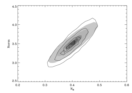
Figure 1: Marginal posterior distributions for the continuum parameters of an absorbed power law fit to an XRT spectrum of GRB 060124. The contours enclose $80$, $50$, $20$, $10$ and $5\%$ of the distribution (and therefore correspond to $20$, $50$, $80$, $90$, $95\%$ credible regions for the parameters). The filled contours were computed assuming the posterior is a Gaussian. The hollow contours were computed using MCMC simulations from the routine of van Dyk et al. (2001). The two distributions are clearly very similar. See section 3.1.3 for details.

As a further test of the Gaussian approximation we compared the posterior calculated using the Laplace approximation with the posterior calculated using the MCMC algorithm discussed in van Dyk et al. (2001). The MCMC method does not use an analytical approximation for the posterior, and therefore is a more general method, but is computationally demanding. Figure 1 illustrates the two posterior distributions calculated for the specific case of a spectrum from GRB 060124. The Gaussian data were computed from $10^{5}$ random draws from a multidimensional Gaussian with a covariance matrix evaluated as the minimum $\chi^{2}$ location using XSPEC. The non-Gaussian data were generated from $10^{5}$ draws generated by the MCMC routine of van Dyk et al. (2001). It is clear that the two distributions are not identical but are very similar both in terms of size and shape. In the present context it is important that the “credible regions” occupy similar volumes of parameter space.

The above analyses demonstrate the Gaussian approximation is reasonable for the posterior of the simple “continuum” model $M_{0}$, which is the denominator of equation 4. The same will be true of the more complex “continuum $+$ line” model $M_{1}$ when the line is well detected (see section 11.3 of Gregory 2005). When the line is weakly detected the posterior will be close to the boundary of the parameter space, in which case the Gaussian approximation will not be so accurate. Indeed, when the MLE of the line normalization is close to the boundary the likelihood (and therefore posterior) enclosed in the allowed region of parameter space will be smaller than that given by the Laplace approximation, which assumes the Gaussian function extends to infinity in all directions. This will also happen, for example, when the best-fitting line energy is near the limit of the allowed energy range. In such cases there will be a tendency to overestimate the Bayes factor (i.e. favor $M_{1}$). But when the line is weak there may be multiple peaks in the likelihood (and posterior) which are not accounted for explicitly in the Laplace approximation. We therefore treat the calculated Bayes factors only as a rough guide to the presence of a spectral line.

3.1.4 Assigning Priors

Bayes factors are sensitive to the choice of prior density. As stated above, using the Laplace approximation the resulting Bayes factors are sensitive to the prior densities only at the MLE parameter values, but we must exercise care in assigning prior density functions in order that these values are reasonable. Fortunately, the prior densities for all parameters that are common to $M_{0}$ and $M_{1}$ (such as photon index and normalization) are the same for $M_{0}$ and $M_{1}$, and therefore cancel out in the ratio. For the other parameters we have no cogent information except for their allowed ranges. In such cases we should use the “least informative” prior densities (see e.g. Loredo 1990; Sivia 1996; Gregory 2005 and references therein for further discussion).

There are wide ranges of possible line energies and redshifts and so the line energy, $E_{line}$ is only constrained to lie within the useful XRT bandpass, typically $0.3-10$ keV. We therefore assigned a uniform prior density $p(E_{\rm line}|M_{1})=1/[E_{\rm max}-E_{\rm min}]$ over this range. For most spectral fits the line width $W$ was initially held fixed at a value below the instrumental resolution, and later allowed as a free parameter. For those models in which the width of the line was a free parameter, the width was assigned a uniform prior over the allowed range (usually $0.0-0.7$ keV): $p(W|M_{1})=1/[W_{\rm max}-W_{\rm min}]$.

In order to test the dependence of the results to the prior densities, two non-informative prior assignments were made for the line strength (normalization), $A$, following the discussion in Gregory (2005). Firstly, following $\S$4.2 of Sivia (1996) the line strength was assigned a uniform prior between zero and some upper limit $A_{\rm max}$. Previous reports of emission lines have estimated the line flux $A$ to be as little as a few percent (Reeves et al. 2002; Watson et al. 2003) or as much as $\sim 40-80\%$ (Yoshida et al. 1999; Piro et al. 2000) of the total flux. We conservatively take $A_{\rm max}$ to be the total flux of the spectrum over the evaluated bandpass (i.e. our constraint is that the line flux is between 0-100% the source flux). However, there are strong arguments (Loredo 1990; Gelman et al. 1995; Gregory 2005) that such as ‘scale’ parameter should be given a Jeffreys prior, $p(A|M_{1})\sim 1/A$, which corresponds to a constant density in $\log(A)$. Formally this is an improper prior (cannot be normalized such that its integral is unity), but one can apply reasonable upper and lower bounds in order to form a proper prior density. Following equation 3.38 of Gregory (2005) we used $p(A|M_{1})=1/A\ln[A_{\rm max}/A_{\rm min}]$. In the present context $A_{\rm max}/A_{\rm min}=800$, since a reasonable lower limit to the X-ray counts from a line is one count, and a reasonable upper limit is $800$, the total number of counts in the spectrum. This yields $p(A|M_{1})=1/6.68A$ as a normalised Jeffreys prior. The prior density is therefore higher for weaker lines in the Jeffreys case compared to the uniform case at values (i.e. over $1.25\times 10^{-3}A_{\rm max}\leq A<0.15A_{\rm max}$), and lower for stronger lines.

The ratio of the prior densities at the modes of the two likelihood functions is then simply

$$\frac{p(\hat{{\mbox{\boldmath$\theta$}}}_{1}|M_{1})}{p(\hat{{\mbox{\boldmath$\theta$}}}_{0}|M_{0})} = p(\hat{E}_{\rm line}|M_{1})p(\hat{W}|M_{1})p(\hat{A}|M_{1})$$ (8)

$$= \frac{1}{([E_{\rm max}-E_{\rm min}][W_{\rm max}-W_{\rm min}]A_{P})},$$

in the ranges $E_{\rm line}\in[E_{\rm min},E_{\rm max}]$, $W\in[W_{\rm min},W_{\rm max}]$ and zero elsewhere. Here, $A_{P}=A_{\rm max}$ in the uniform case or $A_{P}=6.68\hat{A}$ in the Jeffreys case. We have used both uniform and Jeffrey’s priors in the analysis discussed below (see section 6.11).

3.2 Posterior Predictive $p$-values (ppp)

The use of posterior predictive $p$-values (ppp) was advocated, and demonstrated by application to GRB spectra, by Protassov et al. (2002, see $\S$4.1 for a description of their method and $\S$5 for its application to GRB 970508). Like Bayes factors this method is grounded in Bayesian probability theory.

One uses the posterior density, $p({\mbox{\boldmath$\theta$}}|\mathbf{D})$, for the model parameters conditional on the data – which defines our state of knowledge about the parameters given the data and the available prior information – to determine the posterior predictive distribution – which is the distribution of possible future data predicted based on the observed data. (‘Predictive’ because it predicts possible future datasets and ‘posterior’ because the parameters are drawn from the posterior density of the parameters.) The posterior predictive distribution is:

$$p(\mathbf{D}^{\rm sim}|\mathbf{D})=\int p(\mathbf{D}^{\rm sim},{\mbox{\boldmath$\theta$}}|\mathbf{D})d{\mbox{\boldmath$\theta$}}=\int p(\mathbf{D}^{\rm sim}|{\mbox{\boldmath$\theta$}})p({\mbox{\boldmath$\theta$}}|\mathbf{D})d{\mbox{\boldmath$\theta$}}$$ (9)

where $\mathbf{D}^{\rm sim}$ are the possible future datasets (simulations). In practice the posterior density is used to generate a set of random parameter values ${\mbox{\boldmath$\theta$}}_{i}^{\rm sim}$ ($i=1,2,\ldots$) and each of these is used to simulate a random dataset $\mathbf{D}_{i}^{\rm sim}$. The set of simulated data from all the possible random parameters defines the posterior predictive distribution for simulated data. This in turn can be used to define the posterior predictive distribution for some test statistic $T(\mathbf{D})$ (which is a function of the data):

$$p[T(\mathbf{D}^{\rm sim})|\mathbf{D}]=\int p[T(\mathbf{D}^{\rm sim})|{\mbox{\boldmath$\theta$}}]p[{\mbox{\boldmath$\theta$}}|\mathbf{D}]d{\mbox{\boldmath$\theta$}}$$ (10)

(compare with equation 9). The posterior predictive $p$-value (ppp) is the fraction of this distribution for which $T(\mathbf{D}^{\rm sim})>T(\mathbf{D})$, i.e. the area of the tail of the distribution with values of the test statistic more extreme than the value from the observed data.

$$p=\int_{T(\mathbf{D})}^{\infty}p[T(\mathbf{D}^{\rm sim})|\mathbf{D}]d\mathbf{D}^{\rm sim}$$ (11)

where the integration is taken over the posterior predictive distribution of $\mathbf{D}^{\rm sim}$. As such the ppp value is a Bayesian analogue of the $p$-value of null hypothesis tests familiar from classical statistics (e.g. the $F$ or $\chi^{2}$ tests). See chapter 6 of Gelman et al. (1995) or Gelman et al. (1996) for a general discussion of the ppp method, and Protassov et al. (2002) for application to GRB data.

Using the posterior predictive distribution from equation 9 one can produce a large number of random simulated datasets to be used in a Monte Carlo scheme to calculate the integral of equation 11 numerically. The steps for a Monte Carlo method for computing the posterior predictive distribution to calibrate the test statistic $T$ are as follows:

1. Compute the value of the test statistic for the observed data, $T(\mathbf{D})$

2. Randomly draw $N$ sets of $M_{0}$ model parameter values ${\mbox{\boldmath$\theta$}}_{i}$ for $i=1,2,\ldots,N$ according to the appropriate posterior distribution $p({\mbox{\boldmath$\theta$}}|D)$

3. For each of $i=1,2,\ldots,N$ simulate a dataset $\mathbf{D}_{i}^{\rm sim}$ using the randomly drawn parameter values ${\mbox{\boldmath$\theta$}}_{i}$. This accounts for uncertainties in the parameter values.

4. For each of the simulated datasets compute the test statistic $T(\mathbf{D}_{i}^{\rm sim})$. This is the posterior predictive distribution of the test statistic given the observed data $\mathbf{D}$.

5. Compute the posterior predictive $p$-value as the fraction of simulated datasets that gave a test statistic more extreme than that for the observed data:

   $$p=\frac{1}{N}\sum_{i=1}^{N}\Theta[T(\mathbf{D}_{i}^{\rm sim})-T(\mathbf{D})]$$ (12)

   where $\Theta$ is the Heaviside step function which simply counts instances where $T(\mathbf{D}_{i}^{\rm sim})>T(\mathbf{D})$.

The number of simulations, $N$, must be large to ensure a good approximation to the integral of equation 11 (which is a multiple integral, being itself the integral of the function computed by equation 10). See Protassov et al. (2002) for more detailed discussion.

3.2.1 Application to GRB X-ray spectra

As discussed above we may approximate the posterior density for the parameters, using a multidimensional Gaussian centered on the MLE values and with a shape defined by the covariance matrix evaluated at the peak (${\mbox{\boldmath$\sigma$}}^{2}$). The randomised parameter values needed for step $2$ above may then be generated with the Cholesky method.

For the purposes of the present paper we use as the test statistic the change in the $\chi^{2}$ fit statistic between the two models, $M_{0}$ and $M_{1}$. This is equivalent to the formulation discussed in Protassov et al. (2002). The observed data were fitted with the model $M_{0}$ and the covariance matrix evaluated at the best-fit point used to construct the multivariate Gaussian distribution from which parameter values were randomly drawn. For each set of model $M_{0}$ parameter values a spectrum was simulated with the appropriate response matrix and exposure time, with counts in each channel drawn from a Poisson distribution, and binned in the same manner as the observed data.

In order to calculate the test statistic for each simulation, $T(\mathbf{D}_{i}^{\rm sim})$ it was necessary to fit each simulated dataset with the two competing models $M_{0}$ and $M_{1}$, for each one find the best-fitting parameters, and compute $\Delta\chi^{2}_{i}$. This necessarily involves a computationally expensive multi-dimensional parameter estimation for each of the $N$ simulations. We use as standard $N=10^{4}$ simulations which yields a $p$-value accurate to four decimal places at very highest and lowest $p$-values (there is an uncertainty on the ppp value from the finite number of simulations which is roughly $\sqrt{p(1-p)/N}$ from the binomial distribution). This is acceptable for determining $p$-values as low as $p\sim 10^{-4}$, i.e. $99.99\%$ ‘significance’.

As a further test of the validity of the Gaussian assumption for the posterior (see also sections 3.1.2-3.1.3) we have compared results with and without this assumption. In particular, we calculated the ppp-value for a spectrum of GRB 060124 using Gaussian parameter values and also using values generated by the MCMC method discussed by van Dyk et al. (2001). The two results were reasonably close ($p=0.050\pm 0.007$ from the Gaussian simulations and $p=0.073\pm 0.008$ from the MCMC, based on $10^{3}$ simulations). This confirms the point made in section 3.1.3, that the Gaussian assumption is reasonable for these data.

3.2.2 Automated fitting of GRB spectra

Given the number of simulated datasets one must resort to an automated model fitting procedure. This has itself been the cause of some debate, with some authors (e.g $\S$5 of Rutledge & Sako (2003)) claiming that automatic routines do not robustly find the best-fitting parameter values (minimum $\chi^{2}$). The algorithm used by XSPEC for $\chi^{2}$ minimization is the Levenberg-Marquardt algorithm, which is efficient and very effective when the $\chi^{2}$ space is well-behaved (e.g. with only one local minimum). However, as this is a ‘local’ routine there is no guarantee of finding the ‘global’ minimum in $\chi^{2}$, and it is possible that the results are biased by the presence of other local minima. For the present paper we have employed several additions to the standard Levenberg-Marquardt minimization algorithm in order to mitigate these problems.

Once a local minimum in $\chi^{2}$ is found the surrounding region of parameter space is explored for signs of other minima. Each parameter in turn has its value increased and decreased until the $\chi^{2}$ is increased by at least $\Delta\chi^{2}=2.7$, while simultaneously allowing the other parameters to vary in order to minimize $\Delta\chi^{2}$. If any non-monotonicity in $\chi^{2}$ is detected during this search the volume of parameter space explored is increased by increasing the value of $\Delta\chi^{2}$. If during the course of this search $\Delta\chi^{2}$ becomes negative (meaning there is a lower minimum nearby) the Levenberg-Marquardt algorithm is re-started from the position of this new minimum. The entire process is repeated by perturbing each parameter in this way until no further improvement can be made by the adjustment of any of them.

The absorbed power law model ($M_{0}$) has only three parameters (photon index $\Gamma$, normalization and absorption column density), and in all cases finding the $\chi^{2}$ minimum was straightforward using the above procedure. The alternative model $M_{1}$, which includes the emission line, required more care because the presence of a line with unknown energy may cause local $\chi^{2}$ minima at different energies within the wide bandpass. An initial ‘best guess’ line energy was computed for each spectrum in the following way. An absorbed power law plus emission line model was constructed using the best-fitting parameters of model $M_{0}$ and adding an unresolved emission line fixed at some trial energy $E_{i}$ and varying the other parameters (including the line normalization) to find the minimum $\chi^{2}$. One hundred values of the trial energy $E_{i}$ were used, evenly spread over the entire useful bandpass, and the value that recorded the lowest $\chi^{2}$ was selected as the ‘best guess’ for the line energy. The enhanced Levenberg-Marquardt algorithm described above was then used to find the global $\chi^{2}$ minimum starting from this position.

Simulation tests and comparison with interactive fitting demonstrated the automatic procedure described above was an efficient and very robust procedure for finding the global minimum.

3.3 Rutledge and Sako Smoothing (RS)

Rutledge & Sako (2003) proposed an alternative method for line detection using a ‘matched filter’ to smooth the observed count spectrum with the aim of removing low significance noise and emphasizing any spectral features. The distribution of peak fluxes in the smoothed spectrum is then compared to the result of Monte Carlo simulations to calibrate their significance ($p$-value).

The counts per PHA channel are extracted from the observed X-ray spectrum and then smoothed using an energy-dependent kernel (a Gaussian having a FWHM equal to the spectral resolution of the detector; see equation 2 of Rutledge & Sako (2003)) to produce the smoothed spectrum $C(E)$. The distribution of $C(E)$ is then calibrated using Monte Carlo simulations of spectra generated using the method discussed in section 3.2 that employs posterior predictive data sets. (We note that Rutledge & Sako 2003 and Sako et al. 2005 did not randomize the parameter values but used fixed MLE values to generate all their simulations. This is equivalent to assuming the posterior to be a delta function located at the best fit point, which is clearly a bad approximation in many cases.) Each simulation is in turn smoothed using the same energy kernel to produce $C(E)_{sim,i}$. The $C(E)_{sim}$ values are then sorted in descending order for each PHA channel separately. Thus the 99^th percentile limit of the $C(E)_{sim,global}$ is then found by extracting the 100^th highest value of $C(E)_{sim}$ in each PHA channel.

The smoothed observed spectrum, $C(E)$, is then plotted alongside the $n^{th}$ percentile limits, which we have chosen for this analysis to be 90.00, 99.00, 99.90 and 99.99 $\%$. Wherever $C(E)$ exceeds a given limit then we have detected a ‘feature’ at that confidence limit. Thus a line would show up as a narrow excess whilst other thermal emission components will show up as broad excess, both of which are easily distinguishable.

3.4 Comparison of the methods

The three methods discussed above have different theoretical motivations, underlying assumptions and require different amounts of computing power. The Bayes factor method is based on a simple application of Bayes theorem combined with the Laplace approximation and assumes uniform priors on the model parameters (or Jeffreys prior for the line normalization). As discussed above, this may not be the optimal assignment. However, despite its possible drawbacks, the simple priors and Laplace approximation make the calculation extremely simple, requiring only the evaluation of equations 7 and 8 which require the values of $\chi^{2}$ and the covariance matrices for the best-fitting line and line-free models, and details of the free parameters and their allowed ranges. As such, it is useful as a ‘quick and easy’ test. The dependence of choice of priors may be assessed by comparing the results computed using the uniform and Jeffreys prior.

By contrast, the RS and ppp methods require a large number of random datasets to be simulated and analyzed, and are therefore considerably more costly in terms of computing time. There is no compelling theoretical reason for applying a matched filter, as in the RS method, although it should be noted that the method, as implemented above, is calibrated using the appropriate posterior predictive distribution. The advantage of the RS method is that no model fitting is required, which is often a time-consuming process and can lead to biased results if not handled properly (section 3.2.2).

The ppp method is grounded in the theory of Bayesian model checking (Gelman et al. 1995; Protassov et al. 2002) but requires time-consuming fits to be performed on each simulated spectrum, and is therefore the most computationally demanding method by a clear margin. However, it is arguably the most rigorous in the sense that it is less sensitive to the choice of priors than are Bayes factors (Gelman et al., 1996; Protassov et al., 2002), and does not apply an ad hoc smoothing, as in the RS method, that may actually act to suppress real spectral features in some cases.

The simulations used for both RS and ppp methods were generated assuming a Gaussian posterior for the three parameters of $M_{0}$, which, as discussed in section 3.1.3 is a good approximation. Again, this approximation was made to increase computational efficiency, since Gaussian deviates are trivial to generate with the Cholesky method. In situations where the Gaussian approximation is not valid and/or the number of spectra is small enough that considerably more computing time may be spent on each, the ppp method or Bayes factors may be computed using results from MCMC simulations (van Dyk et al., 2001; Protassov et al., 2002) which allows for a more accurate evaluation of the posterior density.

3.4.1 Alternative approximate methods

The statistics literature contains many methods developed for the purpose of model selection. In the introduction we listed four methods that have previously been applied to the problem of line detection in X-ray data from GRBs. One method that has not, to our knowledge, been applied specifically to GRB line detection is the Bayesian Information Criterion (BIC; Schwartz (1978)). This aims to approximate the logarithm of the integrated posterior probability for a model with $k$ parameters given data with a sample size $N$. The BIC takes the form of the logarithm of the likelihood with a penalty term:

$$BIC=-\ln[p(\mathbf{D}|{\mbox{\boldmath$\theta$}},M)]+(k/2)\ln N$$ (13)

The model with the smallest BIC is favored. The difference between the BIC values for two competing models (often called the Schwartz criterion) is therefore $S=-\ln\lambda+(\Delta k/2)\ln N$ (see footnote 8), and is a rough approximation to the logarithm of the Bayes factor (section 4.1.3 of Kass & Raftery 1995).

In the high count (large sample size) limit (see equation 5) the Schwartz criterion becomes $2S=-\Delta\chi^{2}+\Delta k\ln N$. Whether or not the BIC for model $M_{1}$ is smaller than that for $M_{0}$ is then equivalent to the criterion $\Delta\chi^{2}>-\Delta k\ln N$. In the present case the data are selected with fixed $N$, and $\Delta k=-2$ for the addition of a fixed width line, such that the BIC is equivalent to applying the same $\Delta\chi^{2}$ criterion to each spectrum, mechanically the same as the LRT, although with a different (generally higher) threshold value. Therefore, in the present context the application of the BIC would be equivalent to a slightly more conservative application the LRT (see footnote 15). However, as noted in Protassov et al. (2002) and elsewhere, the BIC is often a poor approximation to the integrated posterior probability, and as discussed by Kass & Raftery (1995) is generally a worse approximation than the Laplace approximation employed to calculate Bayes Factors in section 3.1.2.

4 Results from an Iron line emitting source

As a first demonstration of the above methods we applied them to a non-GRB Swift dataset. Ideally we would prefer to examine a source with a GRB-like spectrum, with a similar count rate, but containing a clearly identified emission line feature. However, it is difficult to find a source that meets all of these criteria. We chose the PC mode calibration dataset (combining all available data from 10/05/2005 to 02/09/2005) of PKS 0745-19 (De Grandi & Molendi (1999) and Chen et al. (2003)). This test has some limitations as PKS 0745-19 is fainter than the GRBs analyzed in this paper and it is observed in a different mode.

PKS 0745-19 is a galaxy cluster with a thermal spectrum and a known line at 6.07 keV in Swift’s observations, which is a redshifted 6.7 keV iron line ($z=0.1$). Even though the underlying spectrum is thermal, with multiple temperature components, it can be modeled by an absorbed power law continuum where the power law index, $\Gamma$, is $2.34^{+0.03}_{-0.03}$ ($\chi^{2}/\nu=635/511$). An additional mekal (Mewe et al. (1985) and Arnaud (1996)) component, with kT = $0.19^{+0.03}_{-0.01}$, slightly improved the fit with $\chi^{2}/\nu=610/509$. All spectral parameter errors are quoted at 90$\%$ confidence.

Adding a Gaussian component to an absorbed power law fit naturally produced a significantly improved fit to the data ($\chi^{2}/\nu=539/508$) with $\Gamma=2.36^{+0.04}_{-0.03}$ and a line at $6.07^{+0.02}_{-0.02}$ keV (width = $0.06^{+0.02}_{-0.03}$ keV). The spectral fit to this model can be seen in fig 2. This is supported by the Bayes factor of $7\times 10^{14}$ for a single line being present. RS analysis of the spectrum, fig. 3, also clearly showed the presence of a Gaussian feature at $\sim 6.07$ keV with a significance far in excess of the $99.99\%$ confidence limit. The ppp analysis placed a significance of $>99.99\%$ on this feature.

An interesting point to note is that there are shallow ‘excesses’ at $\sim 0.6$ keV and $\sim 2.3$ keV in the RS plot (fig 3), which are clearly not line features. Coherent, low level, positive excesses are also seen in the spectral fit at these energies (fig. 2). Either the power law component is not modeling the data adequately at these points, the energy scale for this spectrum has an offset or the calibration files are less accurate around these two energies. Applying the gain fit function in XSPEC improves the model fits significantly by adding an offset of -0.07 keV (no change to the slope). The absorbed power law model improves from $\chi^{2}/\nu=635/511$ to $606/509$ and the mekal component model improves from $\chi^{2}/\nu=610/509$ to $585/507$. As a result the two shallow ‘excesses’ at $\sim 0.6$ keV and $\sim 2.3$ keV become far less prominent.

The feature at $\sim 0.6$ keV could be attributed to the detector oxygen absorption edge at 0.54 keV. Applying the -0.07 keV offset brings the $\sim 0.6$ keV ‘line’ in conjunction with this edge, thus reducing its significance below the point at which we would consider it to be a real detection. We note that the $\sim 2.3$ keV feature is coincident in energy with the gold edge due to the XRT mirrors. We have confirmed that this feature is not due to any bad pixel or hot column issues.

5 Testing the three methods and determining detection limits.

In this section we discuss the sensitivity limits of the three methods, i.e. the weakest lines that can be reliably detected with each of the three methods, for observations of the type discussed in section 2, of a ‘typical’ Swift era burst. This is done by simulating XRT data with a continuum spectral model typical of the GRBs observed with Swift, but including an emission line, and then applying the three methods described above for line detection.

In order to generate the simulated data we use a fiducial spectral model comprising a power law with photon index $\Gamma=2.0$, normalization (at 1 keV) of $N=0.9$ photons keV^-1 s^-1 and an absorption column density of $N_{\rm H}=1.8\times 10^{21}$ cm^-2 (see table 2 of Campana et al. 2006c). These parameters are typical of the X-ray spectra of Swift era bursts. In order to measure the sensitivity of the three detection methods to lines in XRT data, spectral data were simulated using the above model plus one Gaussian emission line, and subjected to each of the three procedures. A range of values for line energy, normalization and intrinsic width were used in order to calibrate the dependence of the methods to the line parameters.

The ppp and RS method result in $p$-values with the conventional frequentist interpretation. If we set the detection threshold at $\alpha$, and identify a detection as $p\leq\alpha$ then the rate of type I errors (i.e. false positive detections) will be $\alpha$. For the purpose of sensitivity analysis we used $\alpha=0.01$, equivalent to a “99% significance” criterion. In contrast to these, the Bayes factor is the ratio of the marginal likelihoods of models $M_{1}$ and $M_{0}$; in the case of uniform priors for the two models this is the ratio of posterior probabilities $B_{10}=p(M_{1}|\mathbf{D})/p(M_{0}|\mathbf{D})$ where the probabilities are interpreted directly as probabilities for models $M_{0}$ and $M_{1}$, respectively.

For the purpose of numerical comparison with the $p$-values, the Bayes factors were converted into probabilities (assuming $p(M_{1}|\mathbf{D})+p(M_{0}|\mathbf{D})=1$; see equation 3.19 of Gregory (2005)), and $p(M_{0}|\mathbf{D})<0.01$ was taken as the criterion for detection. This is equivalent to $p(M_{1}|\mathbf{D})>0.99$, and approximately equivalent to a Bayes factor $B_{10}>100$, which is conventionally taken as strong evidence in favor of $M_{1}$ over $M_{0}$ (Kass & Raftery, 1995). However, we stress that the interpretation of $p$-values and Bayes factors are fundamentally different. A $p$-value is the tail area of the probability density function of the test statistic, assuming a null hypothesis ($M_{0}$) is true, and is used to decide whether or not to reject the hypothesis. As such, a $p$-value is not the probability for the model $M_{0}$, instead it corresponds to the frequency of more extreme test statistics (e.g. $\Delta\chi^{2}$) given a large number of repeat experiments (assuming the null hypothesis). By contrast, $p(M_{0}|\mathbf{D})$ is the posterior probability for model $M_{0}$ based on data $\mathbf{D}$ and the priors (in the present case we used an approximation thereof), as $p(M_{1}|\mathbf{D})$ is for $M_{1}$, and Bayes factors are used to select between two models based on the ratio of these two. This fundemental difference in the interpretation of Bayes factors means there is no expectation that $\alpha$ is the frequency of type I errors from a large number of repeat observations when using a $p(M_{0}|\mathbf{D})<\alpha$ criterion.

In $\S$ 3.1.3 we confirmed that using the Laplace approximation assumption in the calculation of the Bayes factor was valid for the fiducial absorbed power law spectral model. The same was also found to be true of the spectra with simulated Gaussian lines at, and above, the detection limit detailed above.

For each value of the line normalization we calculated the Bayes factors for $50$ independent simulations and calculated the $p(M_{0}|\mathbf{D})$ values for each. We then averaged the $p(M_{0}|\mathbf{D})$ values at each normalization and linearly interpolated between points at adjacent normalization values to map $p_{0}$ as a function of normalization. The limiting sensitivity was taken to be the normalization at which the mean $p(M_{0}|\mathbf{D})$ value falls below $0.01$.

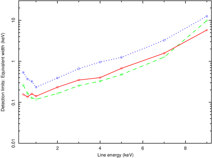
Figure 5: Broad Gaussian line (width = 0.2 keV) for a spectrum containing 800 counts (left) and 1600 counts (right). Comparison of the detection limits, in equivalent width (keV), of the three methods over the energy band pass of Swift. The data are as follows; dotted blue - Bayesian analysis, solid red - RS method, and dashed green - ppp .

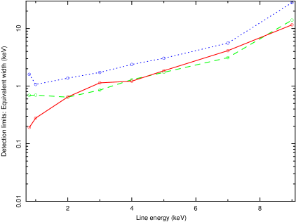
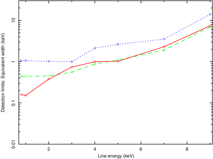
Figure 6: Broad excess (width = 0.7 keV) for a spectrum containing 800 counts (left) and 1600 counts (right). Comparison of the detection limits, in equivalent width (keV), of the three methods over the energy band pass of Swift. The data are as follows; dotted blue - Bayes factor analysis, solid red - RS method, and dashed green - ppp . Values below 0.7 keV have been excluded due to the width of the features being analyzed.

Figure 4 shows the detection limits for an intrinsically narrow line ($W=0$) at different energies for spectra with $\sim 800$ and $\sim 1600$ counts (left and right panels, respectively). The limiting sensitivities are shown in units of equivalent width (keV), which is easier to interpret physically, than the absolute normalization, by comparing the normalization to the underlying continuum model. Figures 5 and 6 show the detection limits for different line widths ($W=0.2$ and $0.7$ keV, respectively). The Bayes factor points in these figures have been calculated using the uniform prior, rather than the Jeffreys prior. See $\S$ 6.11 for further discussion on the effect of using the two different priors in the calcualtion of the Bayes factors for the observed data sets.

The ppp and RS methods require a large number of spectral simulations in order to calibrate their distribution and estimate the $p$-value. The computational demands of this are such that it was not feasible to produce a sufficiently large set of simulations to carry out the methods on each and every line spectrum (e.g. which includes several spectra at each trial value of line energy, width and normalization, for both $\sim 800$ and $\sim 1600$ count spectra). We therefore constructed two libraries of $10^{4}$ simulations, one for $\sim 800$ and one for $\sim 1600$ count spectra, that could be used for each test. These were constructed by simulating an appropriate spectrum based on the fiducial model, and using this to generate the posterior predictive distribution from which to draw $10^{4}$ simulations following the recipe discussed in section 3.1.2. These libraries were then used to calibrate the distribution of the $\Delta\chi^{2}$ statistic for the ppp method and thus to calculate the value of $\Delta\chi^{2}$ that corresponds to a $p$-value of $0.01$. Similarly these libraries were used to compute the 99.00% significance contour from the fiducial model for the RS method. We point out here that these simulation libraries were used only for the purposes of comparing the different algorithms. For the analysis of real observations (discussed below), each observation was assessed using independently generated simulations matching the particular observational parameters.

For the ppp method each of the spectra containing a line was fitted with an absorbed power law with and without an additional Gaussian component, and the change in $\chi^{2}$ noted. The $\Delta\chi^{2}$ values were averaged at each normalization, and these points linearly interpolated, to map the $\Delta\chi^{2}$ as a function of normalization. As with the Bayes factor, the limiting sensitivity was taken to be the normalization at which the mean $p$-value falls below $0.01$, calculated using the appropriated value of $\Delta\chi^{2}$ value from each simulation library. The limiting sensitivity as a function of energy is shown as green dotted curves in Figures 4, 5 and 6 for different configurations of line parameters.

For the RS method each line spectrum was smoothed individually. The $C(E)_{sim}$ values over an energy channel range equal to the central energy, $E_{line}$, $\pm$ line width were extracted. These values were compared to the 99.0% confidence limit over the same energy channel range found from the appropriate simulation library. The number of channels within this range where $C(E)_{sim}>C(E)_{99.0}$ was recorded for each simulation. The detection limit was taken to be the lowest line normalization where $N(C(E)_{sim}>C(E)_{99.0})=0$.

Analysis of the (line free) library simulations showed the Bayes factors produced $<1\%$ false positives when $B_{10}\geq 100$ was used as a detection criterion. This shows the method is, if anything, slightly conservative as expected given the conservative $A_{\rm max}$ assumption. Conversely, the false negative detection rate is negligible above the detection limit.

As expected the detection limits are higher for the spectrum with a lower number of counts, by a factor of $\sim$1.5. For the fiducial spectral model used here the optimum energy range for detecting lines is $0.4-6$ keV, where the line only requires a contribution of a few $\%$ of the total spectral flux, In the best cases ($1600$ counts and narrow line) a line with an equivalent with as small as $\sim 40$ eV may be detected around $1$ keV (observed frame) at $99$% significance (in a single trial), whereas only very strong lines may be detected between $6-10$ keV. Additional simulations were carried out with a higher absorption column density ($1.0\times 10^{22}$ cm^-2; the mean values stated in Reichart & Price (2002) assuming that long bursts occur in molecular clouds). The dependence of line detection with respect to energy for all three methods were the same at energies $>$1 keV. However we note that simulating the spectra with much larger absorption columns significantly degraded the ability to detect lines features below 1 keV.

6 Results from Swift archival GRB afterglow data

Our sample covers a subset of 40 GRBs, out of the total of 153 from GRB 050128 up to GRB 060510B, which were selected for the quality of their WT mode data (see $\S$ 2). Some bursts only contained sufficient data for a single WT mode spectrum to be analyzed, whilst the majority contained sufficient data to be time-sliced into multiple spectra (see $\S$ 2). In total 332 spectra were analyzed. We sample a range of energies and time spans even though the complete redshift distribution of this data set is unknown. The subset of this sample with known $z$ indicates that we are typically probing the region between T+0 s to T+$\sim$500 s (or up to T+few ks if the burst is very bright) post trigger and between $\sim 1.0$ and $\sim 50$ keV in the rest frame of the burst. Throughout this section error bars indicate nominal $90$% confidence limits on one interesting parameter.

All the data were fitted using automated procedure described in section 3.2.2 and the solutions checked by hand. In practice four models were fitted to each spectrum: (1) absorbed power law; (2) absorbed power law plus unresolved Gaussian emission line; (3) absorbed power law plus variable-width line; (4) absorbed power law plus blackbody. The results presented below focus on the line models, and we found that the blackbody parameters were in general very poorly constrained. Ideally, we would like to apply all three methods to all $332$ WT spectra to assess the significance of lines (or other) features in the data. But, as discussed above, the RS and especially ppp methods are computationally demanding and so it was not practical to apply these methods to every spectrum.

The (approximate) Bayes factor method, being computationally economical, was applied to every spectrum, while the more computationally expensive RS and ppp methods were applied only to subsets of the data. In particular, any spectrum that showed a Bayes factor $B_{10}\geq 1$ (in favor of a line), or a $\Delta\chi^{2}\geq 4.61$ upon inclusion of a line, was considered for more detailed analysis. These were deliberately chosen to be extremely relaxed selection criteria (especially so given the large number of independent tests, see below), so as to avoid removing any plausible line candidates and only remove those spectra without any hint of a line, and to counteract the conservative nature of the Bayes factors (section 5). Indeed, this screening effectively reduced by a factor $\sim 4$ the sample of spectra worth considering in more detail. We re-iterate that no judgement about the presence/absence of a line in a spectrum was made purely on the basis of the Bayes factor method, which, as discussed above, is an approximation and is sensitive to the choice of priors. Only spectra with a low Bayes factor ($B_{10}<1$) and little improvement in the fit statistic upon including a line ($\Delta\chi^{2}<4.61$) were not considered for further analysis. This subsample was then subjected to the RS method with a low detection threshold ($p<0.1$, i.e. a $90$% single trial significance, again very weak given the multiple trial effect). This further reduced the sample size to a level where the rigorous but computationally expensive ppp method could be applied.

As stated above, this screening was only necessary to reduce the sample to a manageable size for ppp analysis. Numerical tests showed that the ppp method invariably gave a higher $p$-value (i.e. lower significance) than the RS method, and so no data that might have shown a detection with the rigorous ppp method would have been lost by the selection process.

The large number of spectra examined means the effects of multiple trial must be included in the analysis. For example, to reach a global detection significance of only $90.0$% given a sample of $332$ spectra, we would require a single trial significance in excess of $99.97$%. Of the $332$ spectra from $40$ GRBs, $12$ spectra from $10$ GRBs gave a single trial detection of $\geq 99.9$% significance in at least one of the methods. As the best line candidates in the sample, we now consider each of these in turn. (All significances are single trial values, unless otherwise stated.)

6.1 GRB 050730

A single Gaussian feature was detected in the spectrum extracted from T+692s to T+792s, which was concurrent with a flare in the WT mode data (Starling et al. (2005) and Pandey et al. (2006)). An absorbed power law plus a broad Gaussian ($\sigma=0.34^{+0.08}_{-0.16}$ keV) at $1.14^{+0.48}_{-0.44}$ keV provided the best fit to the data with $\chi^{2}/\nu=47/52$ (table 1). When the line width was restricted to below the detector resolution a Gaussian feature at $0.73^{+0.02}_{-0.03}$ keV was detected ($\chi^{2}/\nu=57/53$).

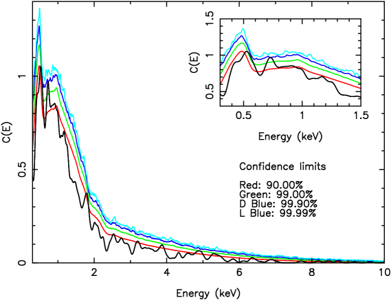
Figure 7: GRB 050730 (T+692s to T+792s): RS method. Inset focuses on energy range of interest.

The Bayes factor was $B_{10}=300$, favoring a line. The RS method (fig. 7) indicated that a line is present in the spectrum at $\sim 0.7$ keV with a confidence of 99.90$\%$. This compares favourably to the parameters found in the spectral fit when the Gaussian width was restricted to a value below the instrumental resolution. There is no evidence for the broader feature found when the width of the Gaussian was a free parameter (see inset to fig. 7).

A ppp analysis was carried out in both cases. The significance of the unresolved-width and free-width Gaussian features were found to be 88.50$\%$ and 99.92$\%$ respectively. It is surprising that the ppp analysis appears to favour the wider line at $E_{\rm line}=1.14^{+0.48}_{-0.44}$ keV, as there is no evidence of a feature with this energy in the RS plot. However, we note that the large errors on this line energy are consistent with a feature at $0.73^{+0.02}_{-0.03}$ keV at the limit of their range.

Applying the gain fit function to this spectrum resulted in an improved fit ($\Delta\chi^{2}=6$) for an unresolved-width line feature at $0.68^{+0.07}_{-0.04}$ keV, with an offset of -55 eV (all other spectral parameters were unchanged within previous limits). Combining this energy offset with the error on the line energy is not sufficient to prove an association with the oxygen absorption edge. Applying the gain fit function to the free-width Gaussian model was inconclusive, with regards to an association to the oxygen absorption feature, owing to the poorly constrained line energy of $<1.00$ keV. (For further discussion on the application of the gain fit function to this and other GRBs see $\S$7.)

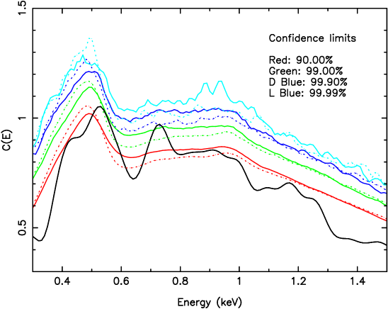
Figure 8: GRB 050730 (T+692s to T+792s): RS comparison between the absorbed power law models containing a single $N_{\rm H}$ component (wabs, dotted lines) and two components (wabs and zwabs, solid lines). Note that the feature becomes far less significant with the addition of the $N_{\rm H}$ column at the appropriate redshift.

The redshift for this burst was reported as $z=3.967$ (Chen et al. (2005), Holman et al. (2005), Prochaska et al. (2005) and Starling et al. (2005)). Further fits were conducted with two $N_{\rm H}$ columns originating from the Galactic column (wabs, fixed at the value given by Dickey & Lockman (1990)) and the host galaxy (zwabs). This had the effect of marginally improving the fit for the absorbed power law model ($\chi^{2}/\nu=61/55$, $\Delta\chi^{2}=3$) with a Galactic column density fixed at $3.21\times 10^{20}$ cm^-2 and a host galaxy component of $9.80^{+6.80}_{-6.20}\times 10^{21}$ cm^-2. All of the other spectral parameters were the same as the previous fit within the limits. The fit to the other models, containing Gaussian components, did not change significantly and the parameter values were the same within the error limits. Bayes factor analysis including the zwabs component indicated marginal evidence for line being present ($B_{10}=5$). Applying the additional zwabs component to the RS method (see fig 8) also decreased the significance of the 0.73 keV feature from 99.90$\%$ confidence (dotted line) to 99.0$\%$ (solid line). A ppp analysis, taking the zwabs component into account, found that the significance of the free-width feature had decreased to 99.49$\%$ (i.e. $\sim 2.8\sigma$ detection) in this single trial. We conclude that the line detection (unresolved or free-width) in GRB 050730 is not significant at 3$\sigma$, and note that the redshift-corrected line energy does not correspond to a K-shell transition of a common element.

6.2 GRB 060109

This burst had insufficient flux to produce multiple spectra therefore we considered the dataset as a whole. The spectrum covers data from T+109s to T+199s. An absorbed power law plus a narrow Gaussian at $0.74^{+0.03}_{-0.03}$ keV (width restricted to below the detector resolution, $\chi^{2}/\nu=40/40$) and a free-width Gaussian at $<0.72$ keV (width = $0.23^{+0.12}_{-0.06}$ keV, $\chi^{2}/\nu=35/39$) were equally good fits to the data (table 1).

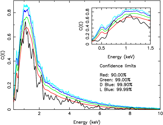
Figure 9: GRB 060109: RS results.

The Bayes factor for the unresolved-width Gaussian model indicated the presence of a line ($B_{10}=200$), however the same analysis on the free-width Gaussian was much less convincing ($B_{10}=3$). The RS method indicated that there may be a feature at $\sim 0.7$ keV with a significance of 99.90$\%$ (see fig 9). However, the ppp method gave only 88.99$\%$ and 99.28$\%$ significance for unresolved (fixed) and free-width Gaussian lines, respectively. In $\S$6.1, we showed that the significance of a similar feature decreased below 3$\sigma$ when the spectral fit was changed to include an absorption component at the redshift of the host galaxy. We will show that this is generally true for those GRBs for which a redshift is known. Unfortunately, in this case, the redshift is not known and we cannot determine whether or not the same is true.

6.3 GRB 060111A

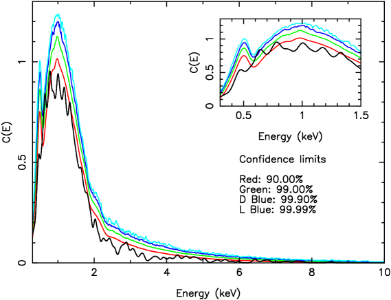
Figure 10: GRB 060111A (T+164s to T+234s): RS results.

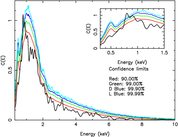
Figure 11: GRB 060111A (T+319s to T+339s): RS results.

The data from this burst were split into 11 spectra, covering several flaring events that showed significant spectral variation during the observation. The Bayes factor ($B_{10}=0.05$) gave no evidence for a free-width line (at $0.65^{+0.09}_{-0.06}$ keV, $W<0.13$ keV) in the spectrum covering T+174s to T+234s, despite it producing a modest improvement in the fit ($\Delta\chi^{2}=8$; table 1). The RS results (fig 10), a feature at $\sim 0.65$ keV with $\geq 99.90\%$ confidence. A further feature at $0.79^{+0.02}_{-0.01}$ keV ($W<0.15$ keV) was detected in the spectrum covering T+319s to T+339s. The Bayes factor indicated that the presence of a line in the second spectrum was unlikely ($B_{10}=0.1$) but the RS method (fig 11) suggested an additional spectral feature.

Whilst the $\sim 0.65$ keV feature for T+174s to T+234s and the $\sim 0.79$ keV feature in the T+319s to T+339s both look promising from the RS method, the ppp analysis showed that they were only 85.13$\%$ and 99.56$\%$ significant, respectively, not strong detections given the number of trials (see above).

6.4 GRB 060115

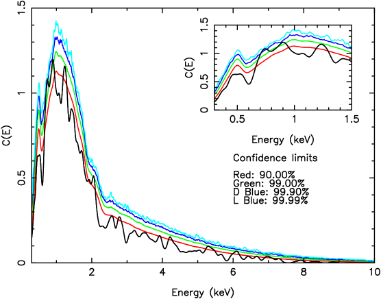
Figure 12: GRB 0601115 (T+121s to T+253s): RS results.

This burst had insufficient flux to produce multiple spectra; therefore we considered the dataset as a whole. The spectrum covers data from T+121s to T+253s. An absorbed power law plus a Gaussian at $0.81^{+0.07}_{-0.07}$ keV with a width of $0.10^{+0.06}_{-0.05}$ keV provided the best fit to the data with $\chi^{2}/\nu=82/77$ (table 1). The Bayes factor gave no evidence for a line ($B_{10}=0.03$), but the RS results (fig. 12) indicated that there was a feature at $\sim 0.75$ keV at the 99.90$\%$ significance. However, ppp analysis gave only 96.16$\%$ significance.

A redshift of $z=3.53$ was reported by Piranomonte et al. (2006). Further fits were conducted with two $N_{\rm H}$ columns originating from the Galactic column (wabs, fixed at the value given by Dickey & Lockman (1990)) and the host galaxy (zwabs). This led to no change in the statistical fit nor parameter values for an absorbed power law model or models containing Gaussian components. We conclude that the line detection in GRB 060115 is only moderately significance in a single trial, and not significant (to 3$\sigma$) in multiple trials, and note that the redshift-corrected line energy does not correspond to a K-shell transition of a common element.

6.5 GRB 060124

A precursor $\sim 570$ s before the main burst peak allowed Swift’s narrow-field instruments to be positioned on the GRB location $\sim 350$ s before the burst occurred (Romano et al., 2006). Therefore the WT mode data covered both the prompt emission from the burst as well as a portion of the afterglow phase. The flux detected over the observation was sufficient to produce a time series containing 46 spectra. Bayes factor analysis indicated that eight of these showed evidence for additional spectral features and a further nine showed evidence from the raw $\Delta\chi^{2}$ improvements. However, RS and ppp analyses carried out on all of these potential line spectra revealed only one with an acceptable detection (with both methods giving a significance of $>99.90\%$). This spectrum spanned T+537s to T+542s (i.e. occurring just prior to the main burst peak). The best fit model to this spectrum was an absorbed power law plus a broad ($\sigma=0.48^{+0.17}_{-0.11}$ keV) Gaussian component at $2.30^{+0.21}_{-0.23}$ keV (table 1).

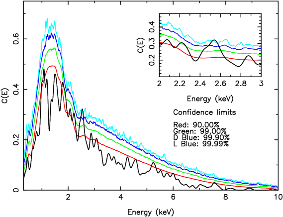
Figure 13: GRB 060124 (T+537s to T+542s): RS results.

The Bayes factor was $B_{10}=20$ for a free-width Gaussian feature in this spectrum. RS results (fig. 13) showed a 99.99$\%$ significance feature at $\sim 2.55$ keV. A ppp analysis indicates that the feature is significant to 99.97$\%$.

Whilst this appears to be a significant detection it seems to be very broad for a single line feature, requiring a velocity dispersion of the order 0.5$c$. Using the redshifts of 0.82 (Mirabal & Halpern, 2006) and 2.297 (Cenko et al., 2006) it is possible to identify this feature with $K_{\alpha}$ emission of Calcium (4.10 keV) or Cobalt (7.5 keV) respectively. It could in principle be a series of unresolved line features, a thermal component or indicating a break in the spectrum. Fitting the spectrum with a blackbody component (kT = $0.76^{+0.14}_{-0.11}$ keV) did not provide a good fit ($\chi^{2}/\nu=61/45$) nor does an absorbed broken power law model ($\chi^{2}/\nu=56/45$).

A further possibility is that it could be due to a poor fit to the gold M-edge as seen in $\S$4. However, applying an energy offset to the data does not significantly improve the absorbed power law model ($\Delta\chi^{2}/\nu=73/45$, offset = -0.08 keV, no change to the slope).

6.6 GRB 060202

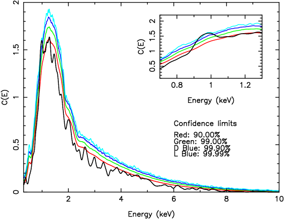
Figure 14: GRB 060202 (T+429s to T+529s): RS results.

This burst contained sufficient flux to extract 18 spectra. Of these spectra only one, spanning T+429 s to T+529 s, appeared to contain an additional spectral feature. The Bayes factor was $B_{10}=300$ in favor of a single free-width line. An absorbed power law plus a broad ($<0.34$ keV) Gaussian feature at $0.94^{+0.05}_{-0.08}$ keV ($\chi^{2}/\nu=96/100$) was a slightly better fit than an absorbed power law alone ($\chi^{2}/\nu=109/103$; see table 1). RS results for the T+429 s to T+529 s data (fig 14) indicated a broad feature at $\sim 0.95$ keV, which exceeds the 99.99$\%$ confidence interval. A ppp analysis of the same data places a significance of 99.74$\%$ on this broad feature. No redshift value has been reported for this burst thus we were unable to perform a well constrained two component absorption fit.

6.7 GRB 060210

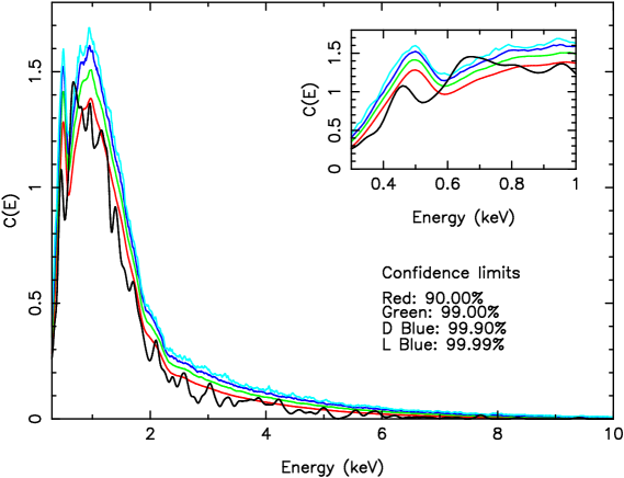
Figure 15: GRB 060210 (T+233s to T+353s): RS results.

This burst contained sufficient flux to extract a time series containing 8 spectra. Of these spectra only one, spanning T+233s to T+353s, appeared to contain an additional spectral feature. A model containing a Gaussian feature at $0.67^{+0.03}_{-0.04}$ keV (width = $0.06^{+0.05}_{-0.03}$ keV) was a much better fit than an absorbed power law alone ($\Delta\chi^{2}=13$; table 1). The Bayes factor was $B_{10}=1$. The RS results (fig 15) indicated that a feature at $\sim 0.65$ keV with a significance of 99.99$\%$. A ppp analysis of the spectrum indicated that the same feature is significant to 99.83$\%$.

A redshift of 3.91 was reported by Cucchiara et al. (2006) for this burst. A two component absorption fit was carried out on the data. This produced a significantly improved fit to the absorbed power law ($\Gamma=2.50^{+0.12}_{-0.11}$) model with a host $N_{\rm H}$ column contribution of $5.65^{+0.85}_{-0.77}\times 10^{22}$ cm^-2 and $\chi^{2}/\nu=80/72$ ($\Delta\chi^{2}=18$ compared to the fit with free Galactic absorption only). Adding a Gaussian component to this gave $\Gamma=2.46^{+0.12}_{-0.12}$, a host absorption column of $5.71^{+0.94}_{-0.83}\times 10^{22}$ cm^-2 and $\chi^{2}/\nu=76/69$ ($\Delta\chi^{2}=5$ compared to the fit with free Galactic absorption only). The addition of the zwabs component did not change the energy of the feature but was only able to place an upper limit of $<0.10$ keV on its width. Bayes factor analysis after allowing for a zwabs component indicated no evidence for an additional spectral feature ($B_{10}=5\times 10^{-4}$). We can conclude that this feature is most likely a false positive detection.

6.8 GRB 060218

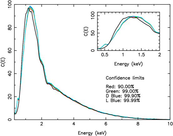
Figure 16: GRB 060218 (T+159s to T+2770s): RS results.

Campana et al. (2006b) have reported on the association of this burst with SN2006aj and the presence of a thermal component in the X-ray spectrum in great detail. Our analysis concurs with their results. The data were split into $53$ time intervals, from which the Bayes factor analysis indicated additional component in the spectrum in all data from $\sim$T+750 s (with $B_{10}>50$). This was confirmed by RS and ppp analysis. The RS results (fig 16, T+159 s to T+2770 s) indicated that this feature is unlikely to be a Gaussian emission line as its profile was too broad. It is possible that it could be a series of unresolved lines, however, a power law plus blackbody component gave the best fit to all of the spectra suggesting an additional spectral feature. Similarly, individual time-slices (see fig 17, T+ 2359 s to T+2409 s, for one such example) show the presence of this broad feature, which appears to evolve over time (Campana et al., 2006b).

6.9 GRB 060418

A time series of 12 spectra were extracted from this GRB, two of which appear to contain additional spectral components. These were the spectra spanning T+119 s to T+129 s and T+169 s to T+194 s.

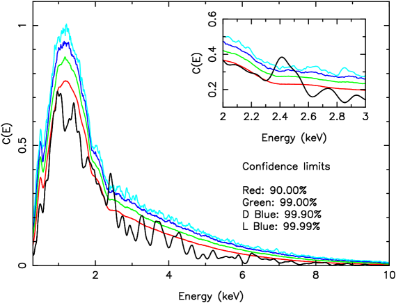
Figure 18: GRB 060418 (T+119s to T+129s): RS results.

A Gaussian component at $2.42^{+0.02}_{-0.03}$ keV improved the fit to the T+119 s to T+169 s data by $\Delta\chi^{2}=16$ (see table 1), although the Bayes factor was unconvincing ($B_{10}=0.05$). The RS analysis (fig. 18) showed a feature at this energy that clearly exceeded the 99.99$\%$ confidence limit. A ppp analysis found 99.85$\%$ significance for the same feature. However, as noted previously in the analysis for GRB 060124 and PKS0745-19 ($\S$4), a feature at this energy is coincident with the gold M-edge.

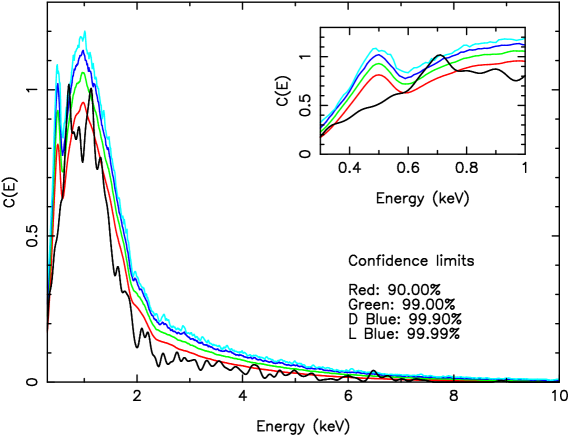
Figure 19: GRB 060418 (T+169s to T+194s): RS results.

A similar improvement in the fit was found for the second spectrum (T+169 s to T+194 s), with $\Delta\chi^{2}=10$, the Bayes factor was more promising ($B_{10}=30$). An unresolved-width Gaussian at $<0.75$ keV provided the best fit to this spectrum with $\chi^{2}/\nu=43/49$ (table 1). RS (fig. 19) and ppp analysis supported the presence of this feature at the 99.99$\%$ and 99.98$\%$ confidence limit respectively.

The 2.42 keV feature of the T+119 s to T+129 s spectrum can be explained by the gold M-edge but the 0.69 keV feature of the T+169 s to T+194 s spectrum cannot be matched to another elemental absorption edge in the same manner. Two component absorption fits were carried out with a $N_{\rm H}$ column density of $9.17\times 10^{20}$ cm^-2 from our Galaxy and a contribution from the host galaxy at $z=1.49$ (Dupree et al. (2006) and Vreeswijk & Jaunsen (2006)). This produced a significant improvement in the absorbed power law model fit, which gave $\Gamma=2.48^{+0.18}_{-0.13}$ and a host $N_{\rm H}=0.73^{+0.23}_{-0.20}\times 10^{22}$ cm^-2 ($\chi^{2}/\nu=53/52$, $\Delta\chi^{2}=9$ compared to the fit with free Galactic absorption only). The addition of a zwabs component to the Gaussian model gave $\Gamma=2.22^{+0.22}_{-0.15}$, a line with an energy of $<0.65$ keV and width of $0.47^{+0.06}_{-0.08}$ keV and a host absorption $<0.21\times 10^{22}$ cm^-2 ($\chi^{2}/\nu=46/49$). The Bayes factor for the spectra containing the zwabs component indicates that the odds of an additional spectral component have been significantly reduced to $B_{10}=1$. We can conclude that this feature is most likely not real, but a spurious detection due to the baseline assumption of no host galaxy absorption.

6.10 GRB 060428B

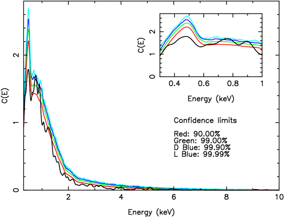
Figure 20: GRB 060428B (T+212s to T+252s): RS results.

Data from this burst were split into two sets, T+212 s to T+252 s and T+252 s to T+418 s. An absorbed power law model was a poor fit to the first spectrum with $\chi^{2}/\nu=78/63$ whilst an absorbed power law plus a Gaussian feature at $0.76^{+0.05}_{-0.06}$ keV (width = $0.09^{+0.05}_{-0.03}$ keV) was a much better fit with $\chi^{2}/\nu=63/60$. However, the Bayes factor was less encouraging with $B_{10}=0.1$ against a line feature. The RS analysis (fig. 20) indicated the presence of two possible features; one at $\sim 0.75$ keV at a significance of 99.99$\%$ and another at $\sim 0.90$ keV at 99.90$\%$. However, no stable spectral fit could be found using an emission line at $\sim 0.9$ keV, hence it was not possible to calculate a Bayes factor, nor calculate the $\Delta\chi^{2}$ needed for a ppp calculation. A ppp analysis of the feature at $0.76^{+0.05}_{-0.06}$ keV yielded a significance of 99.85$\%$.

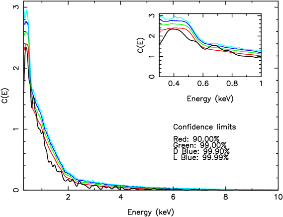
Figure 21: GRB 060428B (T+252s to T+418s): RS results.

The second spectrum, T+252 s to T+418 s, was best fitted by an absorbed power law model ($\chi^{2}/\nu=58/64$, table 1) and the Bayes factor gave only very weak evidence to indicate a line ($B_{10}=3$). RS analysis (fig 21) indicated a possible feature at $\sim 0.7$ keV with a significance of 99.90$\%$, however a ppp analysis placed a much lower significance of 95.87$\%$ on this.

No redshift value has been reported for this burst, preventing us from performing a constrained two component absorption fit. This could potentially determine if the features at $\sim 0.7$ keV are due to poor modeling of the absorption continuum due to not including a component from the host galaxy.

6.11 Use of alternative prior

In section 3.1.4 we discussed two different choices for assigning an uninformative prior to the line normalization. The approximate Bayes factors given above were calculated assuming a uniform prior for the line normalization, but using the Jeffreys prior did not change the results significantly. For example, GRB 060115 changed from $B_{10}=0.03$ with the uniform prior to $B_{10}=0.05$ with the Jeffrey’s prior. At the other extreme, the favorable Bayes factor of $B_{10}=300$ for GRB 060202 (T+[429-529] s) using the uniform prior was virtually unchanged. Spectra that were not included for further analysis, due to a low Bayes factor ($B_{10}<1.0$) and a small $\chi^{2}$ improvement ($\Delta\chi^{2}<4.61$) were similarly affected by a change in priors. In general the Bayes factors changed very little between uniform and Jeffreys priors, reflecting the fact that typical best-fitting line normalizations were usually $\sim 10$% of the total flux (see section 3.1.4).

7 Discussion of Swift XRT results

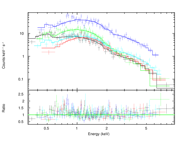
Figure 22: Spectra modeled with an absorbed power law model: GRB 050730 (black), GRB 060109 (red), GRB 060111A (T+174 s to T+234 s, green), 060111A (T+319 s to T+339 s, dark blue) and 060105 (light blue). Note the residuals around 0.7 keV.

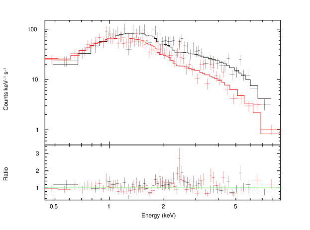
Figure 24: Spectra modeled with an absorbed power law model: GRB 060124 (black) and GRB 060210 (T+119 s to T+129 s, red). Note the residuals around 2.3 keV.

The previous section shows that of 332 WT mode spectra analyzed by our methods only 12 produced possible detections at $\geq$ 99.90% (single trial). These detections were tightly clustered around two energies in the observer frame: 0.64-0.94 kev (10/12, figs 22 and 23) and 2.30-2.49 keV (2/12, fig 24), with equivalent widths of $\sim$0.9 keV and $\sim$0.5 keV respectively.

The coincidence of many spectral feature detections close to 0.7 keV is suspicious as we would expect intrinsic GRB emission line features to be located at different observed energies, as the GRBs span a large range of redshifts. This clustering strongly hints at an instrumental origin. Modeling the WT mode spectra with an energy offset, in case of imperfect bias subtraction at the processing stage, improved the fit statistics for an absorbed power law model (average $\Delta\chi^{2}\sim 5$). However, even if the combined error on the line energy and the offset corrections (1 to 70 eV) are taken, this would still not be enough to provide a plausible association with the oxygen K-edge as seen in the PKS 0745-19 example ($\S$4).

An additional absorption component, at the host galaxy redshift, was applied to those candidates with a known redshift measurement. In every case the feature at 0.7 keV became insignificant and we expect that the same reduction in significance would occur if we were able to conduct well constrained two absorption component fits to the GRBs with unknown redshifts. It could be argued that this decrease in line significance stems only from the increased complexity in the model. If this were the case we should see an overall increase in the level of the RS contours over the whole energy range. In fig 8 we can see that the effect of the adding a zwabs component is not uniform across the energy range. It has negligible effect at energies $>$1.2 keV. Below this energy the zwabs component acts to increase the total absorption at very low energies ($<$0.55 keV) and decrease it in the 0.55 keV to 1.2 keV range. Thus the addition of the second absorption component is imposing a real, energy dependant effect on the confidence contours, rather than increasing them uniformly across the whole energy range. We conclude that the absorption is not being modeled accurately at low energies by assuming that all of the $N_{\rm H}$ column is at a redshift of zero.

We have confirmed that the features at 2.3 keV are not due to bad pixel or hot column issues. The two detections have the following single-trial significances: 99.97% (GRB 060124) and 99.85% (GRB 060418). Taken in the context of all the trials performed these significances become 90.09% ($<1.7\sigma$) and 50.20% ($<0.7\sigma$) respectively. There is no significant impovement to the model fits if the gain fit function is applied. Adding a blackbody component to the underlying absorbed power law or using an absorbed broken power law does not yield a significantly improved fit either. We note, however, that both of these features are coincident with the gold M-edge complex.

Since all of the features are found to be narrowly clustered around two energies in the observer frame, one of which was also found in the PKS 0745-19 example, it is our conclusion that none are real detections of emission lines in GRB spectra, but are instead either due to residual calibration issues, imperfect bias subtraction at the processing stage or incorrect modeling of the host galaxy absorption column (most likely for the 0.7 keV features).

In addition we would expect of the order of 3 false positive detections at 99.00% for 332 spectral analyses.

It is also interesting that the majority of GRBs with potential features occur in the first few months of 2006. There are no physical, instrumental or calibration issues associated with that period of operations that could explain such temporal clustering. However, we note that the actual response of the XRT CCD is possibly evolving while the response is modeled by the calibration files as being constant.

Butler (2007) has recently published analysis citing the detection of line complexes in GRBs 050714B, 050822, 060202 and 060218. However, the same paper and Butler & Kocevski (2007) also provided alternate reasons for these apparent lines detections (thermal components or broken power laws). GRB 050714B was not included in our selection of bursts as the WT mode spectrum did not contain sufficient counts to meet our minimum criteria.

We found no compelling evidence from GRB 050822 using any of our analysis methods to suggest that there were any line features in these data, hence it does not feature in $\S$6. Butler (2007) quotes a significance of 4.4$\sigma$ for a complex of 5 lines (0.81, 0.91, 1.04, 1.23 and 1.49 keV) for one spectrum spanning T+489.5 s to T+509.4 s, with equivalent widths of 82, 142, 194, 221 and 265 eV respectively. We note that the features are spaced 100 eV apart, though no obvious physical explanation for this presents itself. It should be noted that Butler’s spectra ($\sim 500$ counts) is contained within our analysis from T+471 s to T+661 s ($\sim 860$ counts); our spectrum cannot be sub-divided further whilst still being directly comparable to the rest of the data analysis presented in this paper. None of the power law (or cutoff power law) models tested provide a good fit to the data (table 2), though cutoff power laws appear to give a much better fit to the data. Adding a blackbody component to an absorbed power law gave poorly constrained parameters: $\Gamma<1.98$; kT $=0.17^{+0.02}_{-0.02}$; and $N_{\rm H}$ $=4.58^{+5.16}_{-3.08}\times 10^{20}$ cm^-2 ($\chi^{2}/\nu=46/38$).

RS analysis of our spectra compared to a base model of an absorbed cutoff power law shows a feature at $\sim 0.7$ keV at $>99.99\%$ significance. However, ppp analysis only placed a significance of 99.74$\%$ on the same feature. In addition the appearance of a feature at 0.7 keV indicates that the absorption column may not have been modeled accurately, as seen in other bursts in the previous section. As there is no report of a redshift for this burst we cannot confirm this by carrying out a well constrained two component absorption fit.

060202 and 060218 have both been discussed in the previous section. We agree with the presence of a blackbody component in 060218 (Campana et al., 2006b). The single feature found in 060202 only occurred in 1 of the 18 time sliced spectra with a significance of 99.74$\%$ (single trial). If we consider the multiple trials carried out this drops to a significance of $95.4$%. Our analysis indicates that it is a broad feature ($\sigma<0.34$ keV) at 0.9 keV rather than a series of resolved or overlapping lines, however it does occur at the same energy over which Butler (2007) reports 4 individual narrow lines. We find no evidence for the reported feature at $4.70\pm 0.07$ keV.

8 Conclusions

Analysis of the galaxy cluster PKS 0745-19, which has a known 6.07 keV emission line, produced a convincing detection by all methods and also uncovered two further features at 0.6 keV and 2.3 keV. Both features are likely to be due to an energy scale offset that causes the instrumental oxygen and gold absorption edges respectively to be poorly fitted ($\S$ 4). A series of simulations over a range of emission line parameters has allowed us to estimate the sensitivity to Gaussian-like features, both broad and narrow. For all three methods, using GRB parameters typical for Swift bursts, the optimum range for emission line detection was found to be $0.4-6$ keV, with line equivalent widths as low as $\sim 50$ eV detectable in principle from data with only $\sim 1600$ counts.

Of the 332 WT mode spectra from real GRBs, only 12 produced possible detections at $\geq$99.90% (single trial). These were all located around two energies in the observer frame: 0.7 keV (10/12) and 2.3 keV (2/12). The coincidence of many spectral features close to 0.7 keV is suspicious as we would expect intrinsic GRB emission line features to be located at different observed energies, as the GRBs span a large range of redshifts. For those candidates with a redshift measurement the feature at 0.7 keV becomes insignificant once an absorption component at the redshift of the host galaxy is applied. We expect that the same reduction in significance would occur if we were able to apply well constrained two absorption component fits to the GRBs with unknown redshifts. The 2.3 keV features are thought to be associated with the gold M-edge.

Since all of the features are found narrowly clustered around two energies, one of which was also found in the PKS 0745-19 spectrum (2.3 keV), it is our conclusion that all of these features are either due to calibration issues, imperfect bias subtraction at the processing stage or incorrect modeling of the host absorption column (most likely case for the 0.7 keV features), rather than GRB emission line detections. The only non-power law emission component we accept as intrinsic is the blackbody component detected in GRB 060218.

Figure 2: Spectral fit to PKS 0745-19 with an absorbed power law plus a narrow Gaussian emission line model. The redshifted Iron line at 6.07 keV is clearly visible. Note also the residuals at 0.6 keV and 2.3 keV, which are thought to be due to the oxygen and gold edges respectively.

Figure 3: PKS 0745-19: RS method. Confidence contours mark the significance of the spectral features. Red $=90.0\%$, green $=99.0\%$, dark blue $=99.90\%$ and light blue $=99.99\%$. Insets focus on energy ranges of interest.

Figure 4: Narrow Gaussian line (width $<$ instrumental resolution) for a spectrum containing 800 counts (left) and 1600 counts (right). Comparison of the detection limits, in equivalent width (keV), of the three methods over the energy band pass of Swift. The data are as follows; dotted blue - Bayes factor analysis, solid red - RS method, and dashed green - posterior predictive $p$-value analysis.

Table 1: Summary of spectral fits for all candidate spectra.

Modela	Photon	Line energy	Line width	Line norm. ($\times 10^{-2}$	Equiv. width	$N_{\rm H}$	$\chi^{2}/\nu$
	index	(keV)	(keV)	photons cm-2 s-1)	(eV)	($\times 10^{20}$ cm-2)
GRB 050730 (T+692s to T+792s)
1	$2.03^{+0.14}_{-0.13}$	…	…	…	…	$5.84^{+2.32}_{-2.14}$	64/55
2	$1.98^{+0.15}_{-0.13}$	$0.73^{+0.02}_{-0.03}$	$<$ Inst. res.	$0.95^{+0.58}_{-0.57}$	50	$8.88^{+6.57}_{-4.72}$	57/53
3	$1.78^{+0.18}_{-0.19}$	$1.14^{+0.48}_{-0.44}$	$0.34^{+0.08}_{-0.16}$	$22.5^{+7.5}_{-18.5}$	3400	$7.08^{+3.95}_{-4.03}$	47/52
GRB 060109 (T+109s to T+199s)
1	$2.29^{+0.18}_{-0.17}$	…	…	…	…	$31.9^{+5.5}_{-5.0}$	48/42
2	$2.29^{+0.20}_{-0.17}$	$0.74^{+0.03}_{-0.03}$	$<$ Inst. res.	$3.11^{+3.08}_{-1.95}$	94	$34.4^{+6.4}_{-5.6}$	40/40
3	$2.20^{+0.18}_{-0.18}$	$<0.72$	$0.23^{+0.12}_{-0.06}$	$17.5^{+13.8}_{-7.7}$	560	$39.6^{+9.8}_{-7.6}$	35/39
GRB 060111A (T+174s to T+234s)
1	$3.05^{+0.22}_{-0.20}$	…	…	…	…	$29.9^{+4.8}_{-4.5}$	52/50
2	$3.09^{+0.23}_{-0.21}$	$0.64^{+0.03}_{-0.03}$	$<$ Inst. res.	$11.6^{+15.2}_{-4.9}$	73	$32.6^{+5.7}_{-5.1}$	44/48
3	$3.07^{+0.09}_{-0.21}$	$0.65^{+0.09}_{-0.06}$	$<0.13$	$14.0^{+16.0}_{-10.1}$	94	$33.0^{+7.9}_{-5.8}$	44/47
GRB 060111A (T+319s to T+339s)
1	$1.97^{+0.14}_{-0.14}$	…	…	…	…	$18.8^{+3.9}_{-3.6}$	69/61
2	$1.94^{+0.14}_{-0.14}$	$0.79^{+0.02}_{-0.01}$	$<$ Inst. res.	$9.42^{+4.86}_{-4.18}$	80	$19.5^{+4.1}_{-3.9}$	54/59
3	$1.94^{+0.07}_{-0.09}$	$0.79^{+0.02}_{-0.01}$	$<0.15$	$9.42^{+11.9}_{-4.18}$	80	$19.5^{+2.7}_{-2.2}$	54/58
GRB 060115 (T+121s to T+253s)
1	$1.88^{+0.12}_{-0.11}$	…	…	…	…	$16.6^{+3.3}_{-3.1}$	93/80
2	$1.85^{+0.12}_{-0.12}$	$0.89^{+0.03}_{-0.03}$	$<$ Inst. res.	$0.67^{+0.44}_{-0.42}$	39	$16.3^{+3.1}_{-3.2}$	86/78
3	$1.82^{+0.13}_{-0.11}$	$0.81^{+0.07}_{-0.07}$	$0.10^{+0.06}_{-0.05}$	$2.09^{+2.21}_{-1.22}$	100	$17.0^{+4.3}_{-2.7}$	82/77
GRB 060124 (T+537s to T+542s)
1	$1.30^{+0.16}_{-0.14}$	…	…	…	…	$29.5^{+6.7}_{-8.0}$	72/47
2	$1.29^{+0.15}_{-0.15}$	$2.49^{+0.06}_{-0.01}$	$<$ Inst. res.	$11.8^{+6.3}_{-6.5}$	800	$27.8^{+9.3}_{-7.8}$	62/45
3	$1.13^{+0.19}_{-0.24}$	$2.30^{+0.21}_{-0.23}$	$0.48^{+0.17}_{-0.11}$	$57.7^{+42.0}_{-25.2}$	150	$18.3^{+9.7}_{-9.9}$	51/44
GRB 060202 (T+429s to T+529s)
1	$2.16^{+0.11}_{-0.10}$	…	…	…	…	$47.1^{+4.3}_{-4.0}$	109/103
2	$2.15^{+0.11}_{-0.11}$	$0.94^{+0.03}_{-0.02}$	$<$ Inst. res.	$2.69^{+1.51}_{-1.30}$	54	$48.1^{+4.8}_{-4.2}$	97/101
3	$2.12^{+0.10}_{-0.12}$	$0.94^{+0.05}_{-0.08}$	$<0.34$	$4.94^{+5.01}_{-2.80}$	99	$50.0^{+1.1}_{-5.0}$	96/100
GRB 060210 (T+233s to T+353s)
1	$2.72^{+0.16}_{-0.15}$	…	…	…	…	$20.6^{+3.1}_{-2.9}$	98/72
2	$2.71^{+0.16}_{-0.15}$	$0.66^{+0.04}_{-0.02}$	$<$ Inst. res.	$4.63^{+3.06}_{-2.40}$	63	$21.5^{+3.5}_{-3.1}$	85/70
3	$2.68^{+0.18}_{-0.16}$	$0.67^{+0.03}_{-0.04}$	$0.06^{+0.05}_{-0.03}$	$7.06^{+5.94}_{-4.54}$	100	$21.6^{+4.0}_{-3.2}$	81/69
GRB 060418 (T+119s to T+129s)
1	$1.82^{+0.13}_{-0.12}$	…	…	…	…	$24.3^{+5.1}_{-4.6}$	72/59
2	$1.82^{+0.13}_{-0.12}$	$2.42^{+0.02}_{-0.03}$	$<$ Inst. res.	$7.21^{+3.00}_{-2.97}$	190	$23.7^{+5.0}_{-4.6}$	56/57
3	$1.82^{+0.13}_{-0.12}$	$2.42^{+0.02}_{-0.04}$	$<0.14$	$7.21^{+4.74}_{-2.98}$	190	$23.7^{+4.6}_{-4.5}$	56/56
GRB 060418 (T+169s to T+194s)
1	$2.70^{+0.22}_{-0.19}$	…	…	…	…	$22.3^{+4.3}_{-3.9}$	62/52
2	$2.67^{+0.07}_{-0.12}$	$0.69^{+0.02}_{-0.02}$	$<$ Inst. res.	$10.8^{+5.6}_{-5.5}$	58	$22.2^{+2.1}_{-2.0}$	52/50
3	$1.82^{+0.22}_{-0.66}$	$<0.75$	$0.57^{+0.09}_{-0.20}$	$110^{+31}_{-75}$	2300	$11.0^{+0.1}_{-0.1}$	43/49
GRB 060428B (T+212s to T+252s)
1	$3.02^{+0.18}_{-0.16}$	…	…	…	…	$11.6^{+2.6}_{-2.3}$	78/63
2	$2.94^{+0.18}_{-0.16}$	$0.77^{+0.03}_{-0.02}$	$<$ Inst. res.	$3.56^{+1.84}_{-1.87}$	39	$10.6^{+2.6}_{-2.2}$	69/61
3	$2.83^{+0.16}_{-0.16}$	$0.76^{+0.05}_{-0.06}$	$0.09^{+0.05}_{-0.03}$	$8.38^{+4.92}_{-3.69}$	100	$9.21^{+2.37}_{-2.27}$	63/60
GRB 060428B (T+252s to T+418s)
1	$2.64^{+0.14}_{-0.14}$	…	…	…	…	$2.28^{+1.63}_{-1.50}$	58/64
2	$2.58^{+0.15}_{-0.14}$	$0.69^{+0.02}_{-0.03}$	$<$ Inst. res.	$0.62^{+0.37}_{-0.37}$	34	$1.73^{+1.64}_{-1.51}$	50/62
3	$2.33^{+0.14}_{-0.22}$	$<1.07$	$0.33^{+0.06}_{-0.17}$	$9.71^{+5.48}_{-8.19}$	2100	$0.39^{+1.93}_{-0.17}$	48/61

Table 2: Summary of spectral fits for GRB 050822 (T+471 s to T+661 s).

Modela	Photon	High energy	Line energy	Line width	Line norm.	Equiv. width	$N_{\rm H}$	$\chi^{2}/\nu$
	index	cutoff	(keV)	(keV)	($\times 10^{-2}$ photons	(eV)	($\times 10^{20}$
		(keV)			cm-2 s-1)		cm-2)
1	$5.20^{+0.52}_{-0.44}$	…	…	…	…	…	$34.0^{+7.7}_{-6.4}$	90/40
2	$2.84^{+0.57}_{-0.18}$	…	$<0.47$	$0.40^{+0.04}_{-0.07}$	$49^{+10}_{-20}$	240	$<12.2$	49/37
3	$2.27^{+0.57}_{-0.18}$	$0.51^{+0.01}_{-0.01}$	…	…	…	…	$18.0^{+7.1}_{-4.0}$	70/39
4	$2.25^{+0.12}_{-0.12}$	$0.82^{+0.03}_{-0.03}$	$0.68^{+0.04}_{-0.04}$	$0.20^{+0.05}_{-0.04}$	$8.50^{+1.64}_{-1.64}$	300	$9.51^{+0.86}_{-0.79}$	55/36

Figure 17: GRB 060218 (T+2359s to T+2409s): RS results.

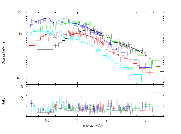
Figure 23: Spectra modeled with an absorbed power law model: GRB 060202 (black), GRB 060210 (red), GRB 060418 (T+169 s to T+194 s, green), 060428B (T+212 s to T+252 s, dark blue) and 060428B (T+252 s to T+418 s, light blue). Note the residuals around 0.7 keV.

Facilities: Swift.

References

- Amati et al. (2000) Amati, L., Frontera, F., Vietri, M., et al. 2000, Science, 290, 953
- Antonelli et al. (2000) Antonelli, L. A., Piro, L., Vietri, M., et al. 2000, ApJ, 545, L39
- Arnaud (1996) Arnaud, K. A. 1996, in ASP Conf. Ser. 101: Astronomical Data Analysis Software and Systems V, ed. G. H. Jacoby & J. Barnes, 17–+
- Ballantyne & Ramirez-Ruiz (2001) Ballantyne, D. R. & Ramirez-Ruiz, E. 2001, ApJ, 559, L83
- Brainerd et al. (1994) Brainerd, J. J., Paciesas, W. S., Meegan, C. A., & Fishman, G. J. 1994, in AIP Conf. Proc. 307: Gamma-Ray Bursts, ed. G. J. Fishman, 122
- Burrows et al. (2005a) Burrows, D. N., Hill, J. E., Nousek, J. A., et al. 2005a, Space Science Reviews, 120, 165
- Burrows et al. (2005b) Burrows, D. N., Romano, P., Falcone, A., et al. 2005b, Science, 309, 1833
- Butler et al. (2005) Butler, N., Ricker, G., Vanderspek, R., et al. 2005, ApJ, 627, L9
- Butler (2007) Butler, N. R. 2007, ApJ, 656, 1001
- Butler & Kocevski (2007) Butler, N. R. & Kocevski, D. 2007, ApJ, 663, 407
- Campana et al. (2006a) Campana, S., Beardmore, A. P., Cusumano, G., & Godet, . 2006a, Swift XRT CALDB Release Notes, 1
- Campana et al. (2006b) Campana, S., Mangano, V., Blustin, A. J., et al. 2006b, Nature, 442, 1008
- Campana et al. (2006c) Campana, S., Romano, P., Covino, S., et al. 2006c, A&A, 449, 61
- Cenko et al. (2006) Cenko, S. B., Berger, E., & Cohen, J. 2006, GRB Coordinates Network, 4592, 1
- Chen et al. (2005) Chen, H.-W., Thompson, I., Prochaska, J. X., & Bloom, J. 2005, GRB Coordinates Network Circular, 3709, 1
- Chen et al. (2003) Chen, Y., Ikebe, Y., & Böhringer, H. 2003, A&A, 407, 41
- Cucchiara et al. (2006) Cucchiara, A., Fox, D. B., & Berger, E. 2006, GRB Coordinates Network Circular, 4729, 1
- De Grandi & Molendi (1999) De Grandi, S. & Molendi, S. 1999, A&A, 351, L45
- Dickey & Lockman (1990) Dickey, J. M. & Lockman, F. J. 1990, ARA&A, 28, 215
- Dupree et al. (2006) Dupree, A. K., Falco, E., Prochaska, J. X., Chen, H.-W., & Bloom, J. S. 2006, GRB Coordinates Network Circular, 4969, 1
- Eadie et al. (1971) Eadie, W. T., Drijard, D., James, F. E., Roos, M., & B., S. 1971, Statistical methods in experimental physics (Amsterdam: North-Holland, 1971)
- Freeman et al. (1999) Freeman, P. E., Graziani, C., Lamb, D. Q., et al. 1999, ApJ, 524, 753
- Frontera et al. (2004) Frontera, F., Amati, L., Zand, J. J. M. i., et al. 2004, ApJ, 616, 1078
- Galama et al. (1998) Galama, T. J., Vreeswijk, P. M., van Paradijs, J., et al. 1998, Nature, 395, 670
- Gehrels et al. (2004) Gehrels, N., Chincarini, G., Giommi, P., et al. 2004, ApJ, 611, 1005
- Gelman et al. (1995) Gelman, A., Carlin, J. B., Stern, H. S., & B., R. D. 1995, Bayesian Data Analysis (London: Chapman & Hall)
- Gelman et al. (1996) Gelman, A., Meng, X.-L., & Stern, H. S. 1996, Statistica Sinica, 6, 733
- Ghisellini & Celotti (1999) Ghisellini, G. & Celotti, A. 1999, ApJ, 511, L93
- Gregory (2005) Gregory, P. C. 2005, Bayesian Logical Data Analysis for the Physical Sciences (Cambridge, UK: Cambridge University Press)
- Hjorth et al. (2003) Hjorth, J., Sollerman, J., Møller, P., et al. 2003, Nature, 423, 847
- Holman et al. (2005) Holman, M., Garnavich, P., & Stanek, K. Z. 2005, GRB Coordinates Network Circular, 3716, 1
- Kass & Raftery (1995) Kass, R. E. & Raftery, A. E. 1995, J. Am. Stat. Ass., 90, 773
- Lazzati et al. (2004) Lazzati, D., Rossi, E., Ghisellini, G., & Rees, M. J. 2004, MNRAS, 347, L1
- Lee (1989) Lee, P. M. 1989, Bayesian Statistics: An Introduction (New York: Halsted Press)
- Loredo (1990) Loredo, T. J. 1990, in Maximum-Entropy and Bayesian Methods, Dartmouth., ed. P. Fougere (Dordrecht, The Netherlands: Kluwer Academic Publishers), 81–142
- Loredo (1992) —. 1992, in Statistical Challenges in Modern Astronomy, Springer-Verlag., ed. D. Feigelson & G. Babu (New York: Springer-Verlag), 275–297
- Mewe et al. (1985) Mewe, R., Gronenschild, E. H. B. M., & van den Oord, G. H. J. 1985, A&AS, 62, 197
- Mirabal & Halpern (2006) Mirabal, N. & Halpern, J. P. 2006, GRB Coordinates Network, 4591, 1
- Morrison & McCammon (1983) Morrison, R. & McCammon, D. 1983, ApJ, 270, 119
- Pandey et al. (2006) Pandey, S. B., Castro-Tirado, A. J., McBreen, S., et al. 2006, A&A, 460, 415
- Pian et al. (2006) Pian, E., Mazzali, P. A., Masetti, N., et al. 2006, Nature, 442, 1011
- Piran (2005) Piran, T. 2005, Reviews of Modern Physics, 76, 1143
- Piranomonte et al. (2006) Piranomonte, S., D’Elia, V., Fiore, F., et al. 2006, GRB Coordinates Network Circular, 4520, 1
- Piro et al. (1999) Piro, L., Costa, E., Feroci, M., et al. 1999, ApJ, 514, L73
- Piro et al. (2000) Piro, L., Garmire, G., Garcia, M., et al. 2000, Science, 290, 955
- Press et al. (1992) Press, W. H., Teukolsky, S. A., Vetterling, W. T., & Flannery, B. P. 1992, Numerical recipes in FORTRAN. The art of scientific computing (Cambridge: University Press, —c1992, 2nd ed.)
- Prochaska et al. (2005) Prochaska, J. X., Chen, H.-W., Bloom, J. S., et al. 2005, GRB Coordinates Network Circular, 3732, 1
- Protassov et al. (2002) Protassov, R., van Dyk, D. A., Connors, A., Kashyap, V. L., & Siemiginowska, A. 2002, ApJ, 571, 545
- Rees & Mészáros (2000) Rees, M. J. & Mészáros, P. 2000, ApJ, 545, L73
- Reeves et al. (2002) Reeves, J. N., Watson, D., Osborne, J. P., et al. 2002, Nature, 416, 512
- Reichart & Price (2002) Reichart, D. E. & Price, P. A. 2002, ApJ, 565, 174
- Romano et al. (2006) Romano, P., Campana, S., Chincarini, G., et al. 2006, A&A, 456, 917
- Rutledge & Sako (2003) Rutledge, R. E. & Sako, M. 2003, MNRAS, 339, 600
- Sako et al. (2005) Sako, M., Harrison, F. A., & Rutledge, R. E. 2005, ApJ, 623, 973
- Schwartz (1978) Schwartz, G. 1978, Ann. Stat., 6, 461
- Shaviv & Dar (1995) Shaviv, N. J. & Dar, A. 1995, ApJ, 447, 863
- Shemi (1994) Shemi, A. 1994, MNRAS, 269, 1112
- Sivia (1996) Sivia, D. S. 1996, Oxford Univ. Press (Oxford)
- Stanek et al. (2003) Stanek, K. Z., Matheson, T., Garnavich, P. M., et al. 2003, ApJ, 591, L17
- Starling et al. (2005) Starling, R. L. C., Vreeswijk, P. M., Ellison, S. L., et al. 2005, A&A, 442, L21
- Tavecchio et al. (2004) Tavecchio, F., Ghisellini, G., & Lazzati, D. 2004, A&A, 415, 443
- Tyler et al. (2006) Tyler, L., Page, K., Goad, M., & Osborne, J. 2006, in ASP Conf. Ser. 351: Astronomical Data Analysis Software and Systems XV, ed. C. Gabriel, C. Arviset, D. Ponz, & S. Enrique, 97
- van Dyk et al. (2001) van Dyk, D. A., Connors, A., Kashyap, V. L., & Siemiginowska, A. 2001, ApJ, 548, 224
- Vietri et al. (2001) Vietri, M., Ghisellini, G., Lazzati, D., Fiore, F., & Stella, L. 2001, ApJ, 550, L43
- Vreeswijk & Jaunsen (2006) Vreeswijk, P. & Jaunsen, A. 2006, GRB Coordinates Network Circular, 4974, 1
- Watson et al. (2003) Watson, D., Reeves, J. N., Hjorth, J., Jakobsson, P., & Pedersen, K. 2003, ApJ, 595, L29
- Watson et al. (2002) Watson, D., Reeves, J. N., Osborne, J., et al. 2002, A&A, 393, L1
- Waxman (1997) Waxman, E. 1997, ApJ, 485, L5
- Yoshida et al. (1999) Yoshida, A., Namiki, M., Otani, C., et al. 1999, A&AS, 138, 433
- Zhang (2007) Zhang, B. 2007, Chinese Journal of Astronomy and Astrophysics, 7, 1