Velocity Structure in the Orion Nebula.
II. Emission Line Atlas of Partially Ionized
to Fully Ionized Gas

Presentamos un atlas de espectros tridimensionales (posición-posición-velocidad) de la Nebulosa de Orión en líneas de emisión ópticas de una variedad de diferentes etapas de ionización: [O 1] 6300 Å, [S 2] 6716,6731 Å, [N 2] 6584 Å, [S 3] 6312 Å, $\mathrm{H}\alpha$ 6563 Å, y [O 3] 5007 Å. Estas transiciones nos dan información punto a punto sobre la estructura física y cinemática de la nebulosa a una resolución efectiva de $3\arcsec\times 2\arcsec\times 10\leavevmode\nobreak\ \mathrm{km\ s}^{-1}{}$, mostrando claramente el comportamiento a gran escala del gas ionizado y la presencia de fenomenos localizados tales como flujos colimados relacionados a objetos Herbig-Haro. Como un ejemplo de la aplicación del atlas presentamos un análisis estadístico de los anchos de las líneas de $\mathrm{H}\alpha$, [O 3] y [N 2], que permiten una determinación de la temperatura electrónica media en la nebulosa de $(9200\pm 400)$ K. También, a diferencia a trabajos anteriores, encontramos que no hay diferencia entre el ensanchamiento no térmico de las líneas de recombinación y el de las líneas colisionales.

Abstract

We present an atlas of three-dimensional (position-position-velocity) spectra of the Orion Nebula in optical emission lines from a variety of different ionization stages: [O 1] 6300 Å, [S 2] 6716,6731 Å, [N 2] 6584 Å, [S 3] 6312 Å, $\mathrm{H}\alpha$ 6563 Å, and [O 3] 5007 Å. These transitions provide point to point information about the physical structure and kinematics of the nebula at an effective resolution of $3\arcsec\times 2\arcsec\times 10\leavevmode\nobreak\ \mathrm{km\ s}^{-1}{}$, clearly showing the large scale behavior of the ionized gas and the presence of localized phenomena such as Herbig-Haro outflows. As an example application of the atlas, we present a statistical analysis of the widths of the $\mathrm{H}\alpha$, [O 3], and [N 2] lines that permits a determination of the mean electron temperature in the nebula of $(9200\pm 400)$ K. We also find, in contradiction to previous claims, that the non-thermal line broadening is not significantly different between recombination lines and collisional lines.

H II regions ISM: Herbig-Haro objects ISM: Herbig-Haro objects ISM: individual: Orion nebula techniques: spectroscopy turbulence

0.1 Introduction

The Orion nebula, M42, is the nearest and best studied high-mass star-forming region in our galaxy (see O’Dell, 2001, and references therein). It is being ionized by a compact group of high-mass stars known as the Trapezium, which was created in the first of three recent epsiodes of star formation that have occured within a region of size one-tenth of a parsec at the center of the Orion Nebula Cluster. The other two star formation episodes, associated with the BN/KL and Orion South regions, are still ongoing and are ocurring in dense molecular gas that lies behind the ionized nebula. The O7 V star $\theta^{1}$ Ori C (Simón-Díaz et al., 2006) is the most luminous and hottest star of the Trapezium and it is responsible for the main ionization front. Many morphological features in Orion that are apparent in emission lines, such as arcs and filaments are associated with collimated gas flows from star-forming activity, such as Herbig-Haro (HH) objects (e.g., Reipurth & Bally, 2001). Jets, bright bars, proplyds and a myriad of other features are conspicuous in optical emission lines making of Orion an ideal laboratory for studying photoionization and hydrodynamic phenomena. Previous high spectral resolution studies over restricted regions in Orion (e.g., Castañeda, 1988; Wen & O’Dell, 1993; Esteban et al., 1998; Baldwin et al., 2000) indicate the presence of complex line profiles; the changing complexity of the emission line profiles over distinct regions of Orion can now be fully appreciated and clearly identified with various phenomena over the entire region covered by our observations.

In this paper we present a comprehensive atlas of high-resolution echelle slit spectra in multiple emission lines, covering a $3^{\prime}\times 5^{\prime}$ region in the center of the Orion nebula. The atlas combines results from two separate datasets, one obtained at Kitt Peak National Observatory (KPNO), and the other from the Observatorio Astronómico Nacional at San Pedro Mártir, B.C., Mexico (SPM). Between them, these datasets, which have comparable spatial and spectral resolution, span a wide range of ionization stages, going from [O 1] 6300 Å, which traces partially ionized gas at the ionization front, up to [O 3] 5007 Å, which traces the most highly ionized gas in the interior of the nebula. Figures and data from the atlas are publicly available from the web page http://www.astrosmo.unam.mx/~w.henney/orionatlas.

Various aspects of the data presented here have been discussed in previous papers: Doi et al. (2004, hereafter Paper I) concentrated on the high-velocity features associated with stellar jets; Henney et al. (2005) analysed the large-scale nebular structure and kinematics in terms of numerical simulations of champagne flows; García-Díaz & Henney (2007, hereafter Paper I) investigated the global structures found in low-velocity emission from low-ionization gas; Henney et al. (2007) analysed the structure and dynamics of the low-excitation jet, HH 528. However the full set of individual long-slit spectra are shown here for the first time and the usefulness and applicability of this comprehensive data set goes beyond the analysis of the previous papers. As example applications of the atlas data, we calculate velocity moment maps of the nebula in each emission line and present a comprehensive analysis of the line profile statistics.

The structure of the paper is as follows. In § 0.2 we present the atlas of slit spectra. In § 0.3 we summarise the spatial variations in line profiles across the face of the nebula by means of maps of integrated line quantities, such as centroid velocity and linewidth. In § 0.4 we analyse the statistical properties of the velocity field in the nebula, including correlations between the kinematics in different emission lines. In § 0.5 we derive the nebular electron temperature from the difference in linewidths of $\mathrm{H}\alpha$ and [O 3]. In § 0.6 we discuss our results in the light of previous work. in § 0.7 we present our conclusions.

0.2 The Atlas

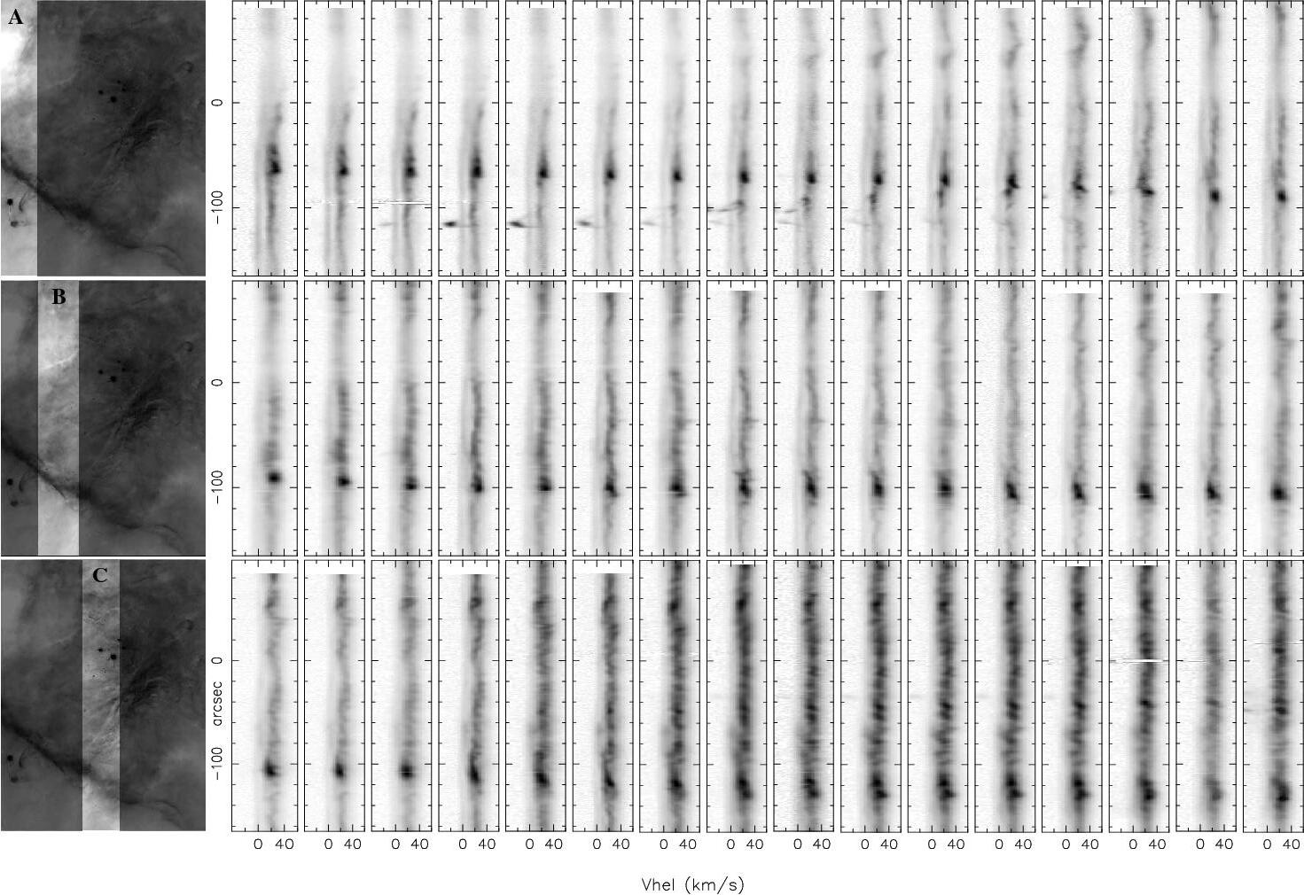
Figure 1: [S 2] 6731 Å individual long-slit spectra are presented as position-velocity (P-V) arrays. For every P-V array the vertical axis covers a range of 250 in declination, while the horizontal axis from $-$40 to $+$60 $\mathrm{km\ s}^{-1}$ in heliocentric velocity. The strip of sky corresponding to the slits in each row is highlighted on an HST image of Orion, shown in the first column. The spectra in the top row (A) are from Kitt Peak (resolution, R, $\approx$ 8 $\mathrm{km\ s}^{-1}$), exept for P-V’s 11, 15 & 16 that are from SPM (R $\approx$ 6 $\mathrm{km\ s}^{-1}$). All other spectra in the middle and bottom rows (B & C) are from SPM (R $\approx$ 12 $\mathrm{km\ s}^{-1}$)

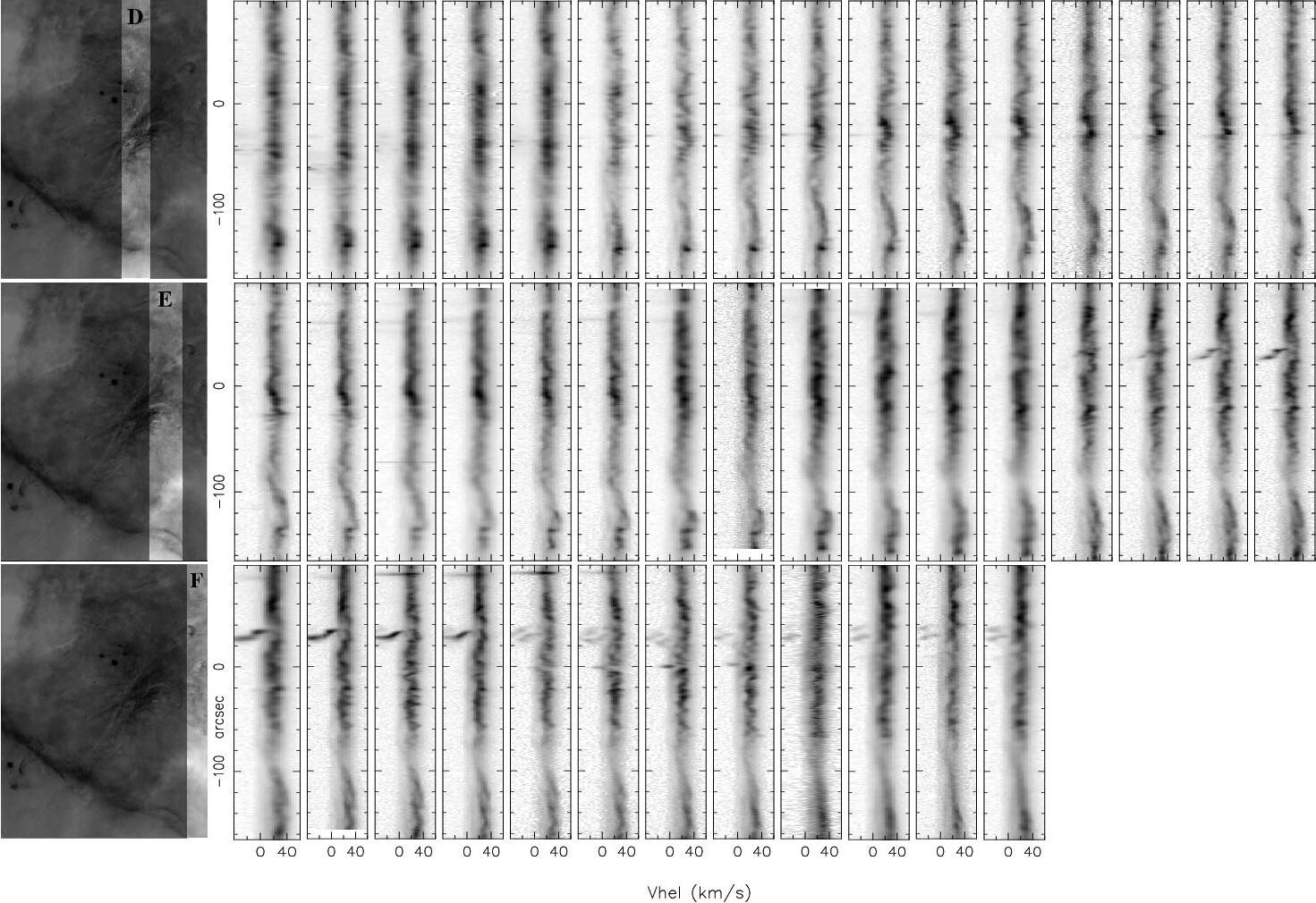
Figure 2: As Figure 1. In strip D the P-V arrays 6 to 16 are from KPNO, the rest are from SPM. In strip E, P-V arrays 1,2,6,13 to 16 are from KPNO, the rest are from SPM. In strip F, P-V arrays 3 and 5 to 9 are from KPNO, the rest are from SPM

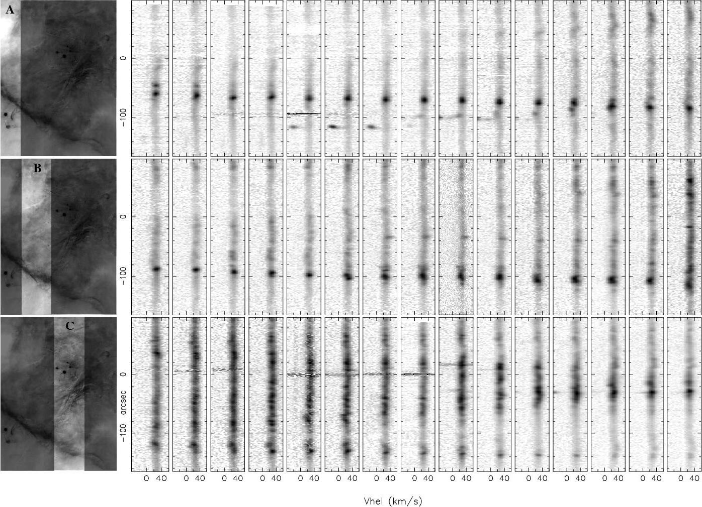
Figure 3: As in Figure 1 but for [O 1] 6300 Å. All the P-V arrays here are from SPM obtained at R $\approx$ 12 $\mathrm{km\ s}^{-1}$, except P-V 9 in strip B, obtained at R $\approx$ 6 $\mathrm{km\ s}^{-1}$

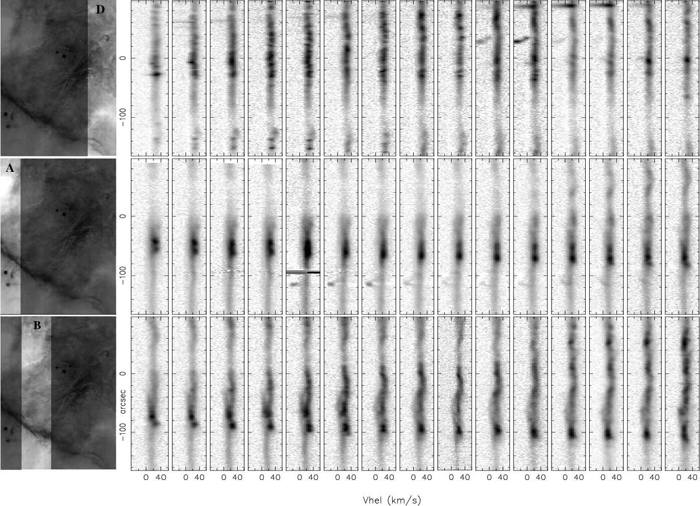
Figure 4: Strip D, top row, shows continuation of [O 1] 6300 Å mapping, as in Figure 3. The P-V arrays in the middle and bottom rows (A & B) correspond to emission from [S 3] 6312 Å, all the spectra are from SPM obtained at R $\approx$ 12 $\mathrm{km\ s}^{-1}$, except P-V 9 in the bottom row, obtained at R $\approx$ 6 $\mathrm{km\ s}^{-1}$

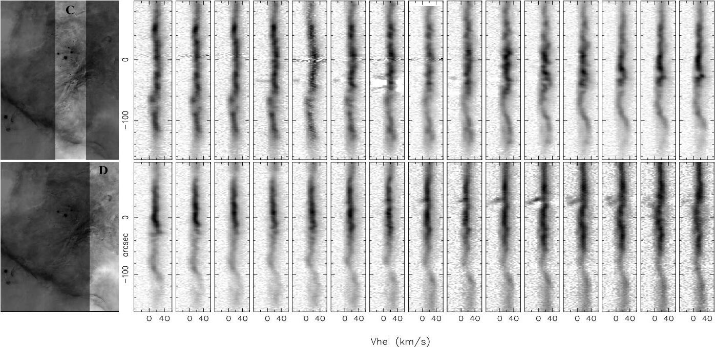
Figure 5: P-V arrays of [S 3] 6312 Å, continued from Figure 4

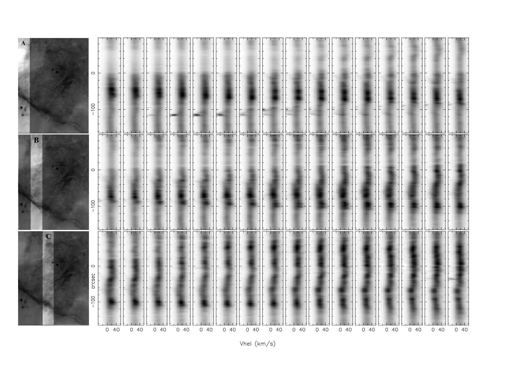
Figure 6: As Figure 1 but for $\mathrm{H}\alpha$ 6563 Å.

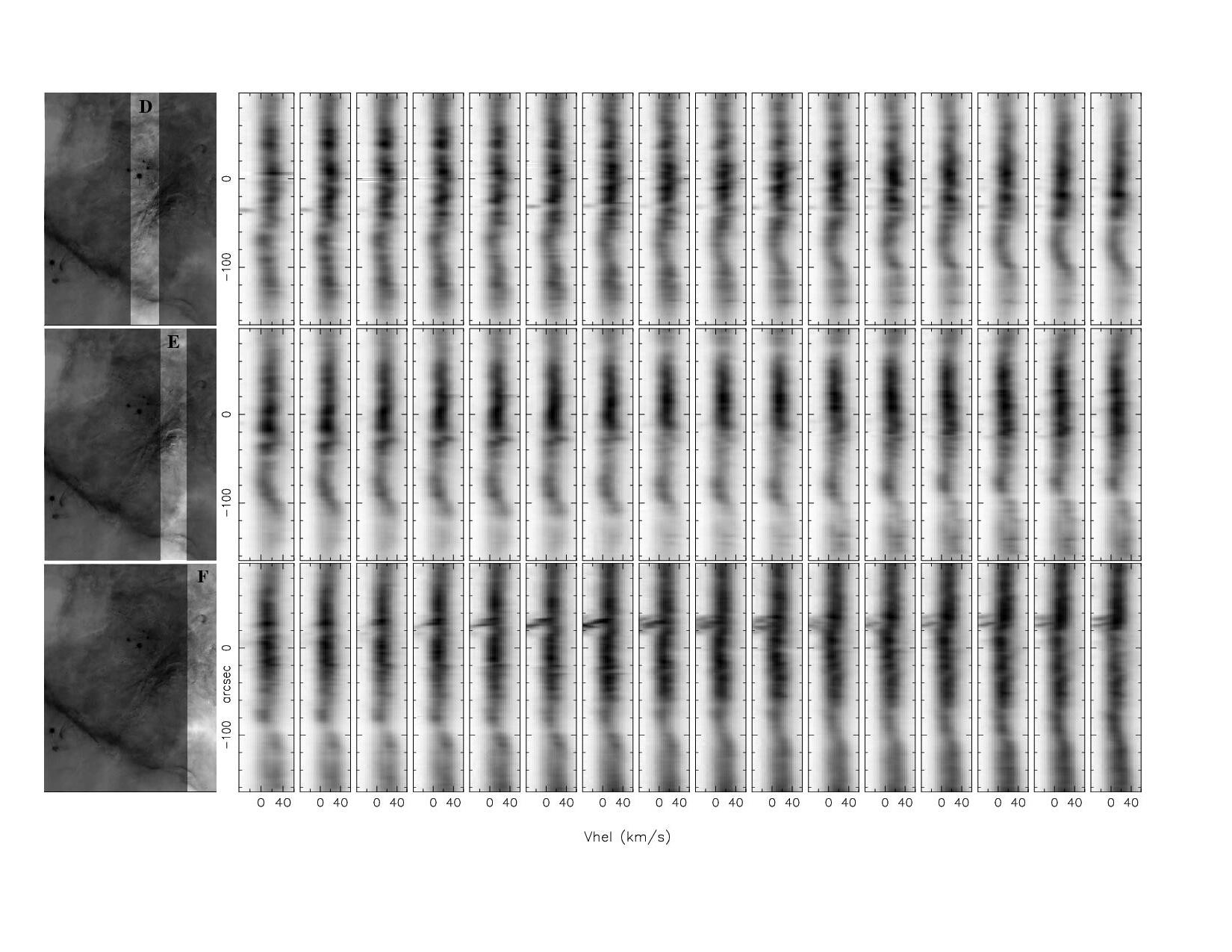
Figure 7: As Figure 1 but for $\mathrm{H}\alpha$ 6563 Å, continued.

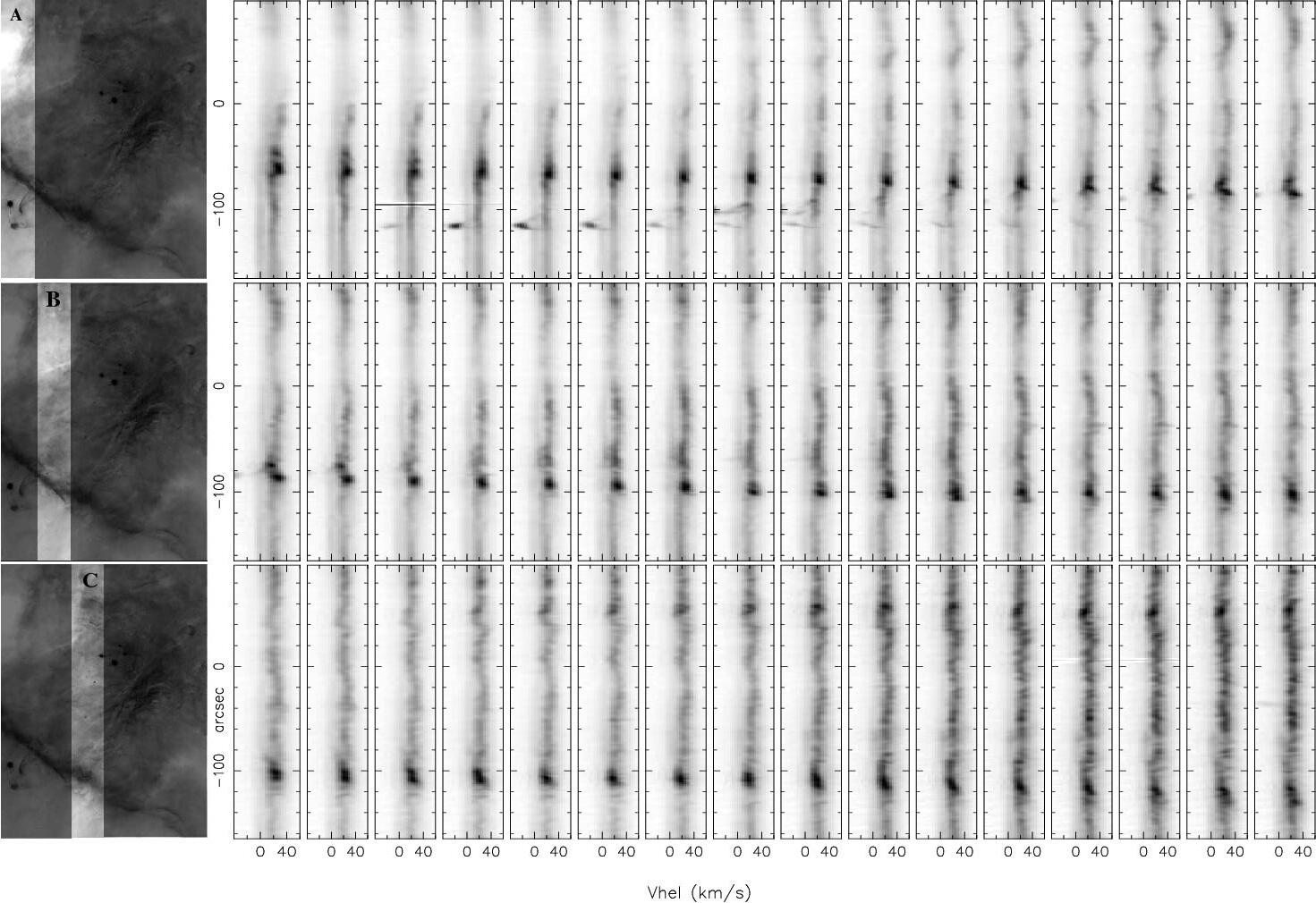
Figure 8: As Figure 1 but for [N 2] 6584 Å.

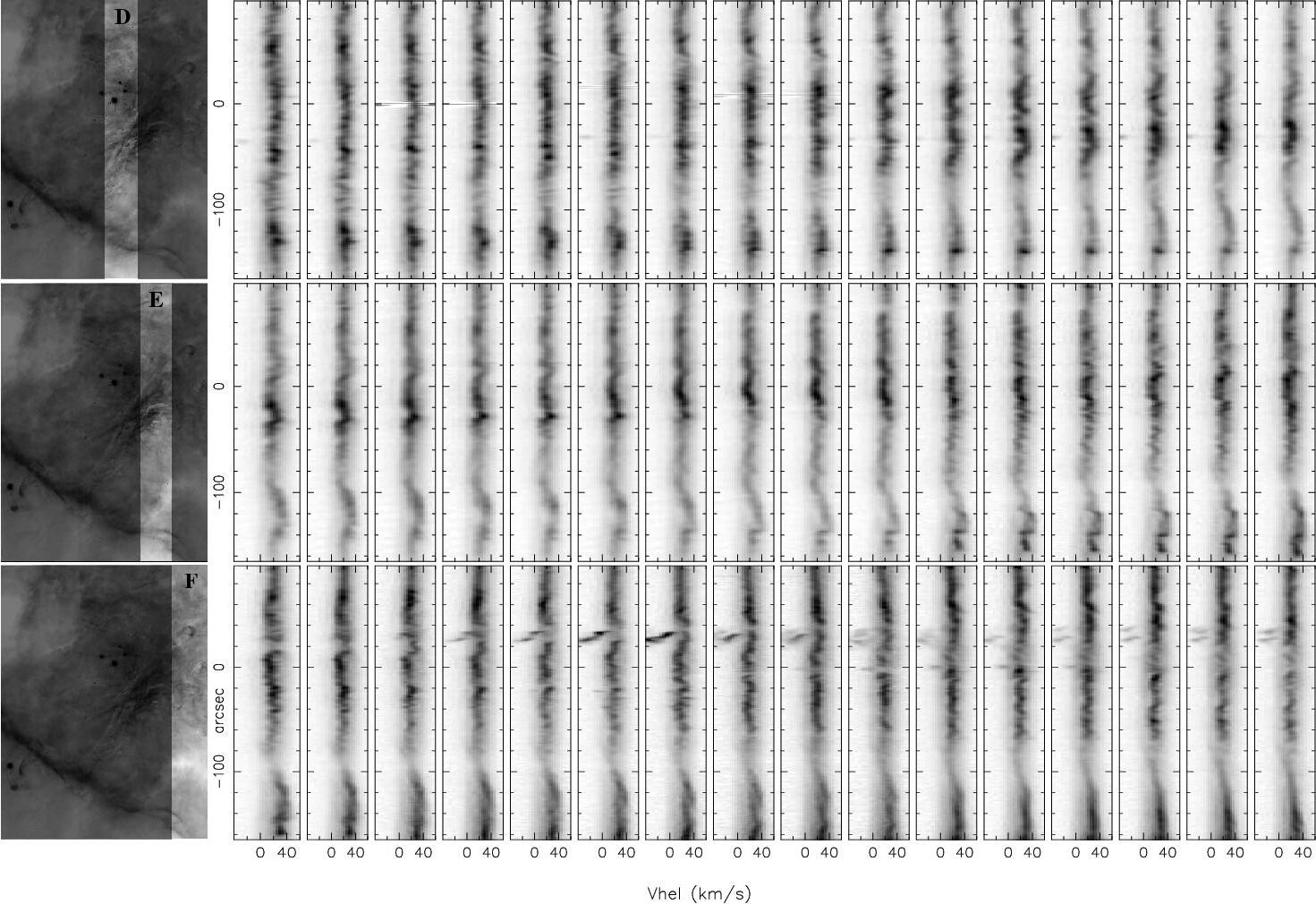
Figure 9: As Figure 1 but for [N 2] 6584 Å, continued.

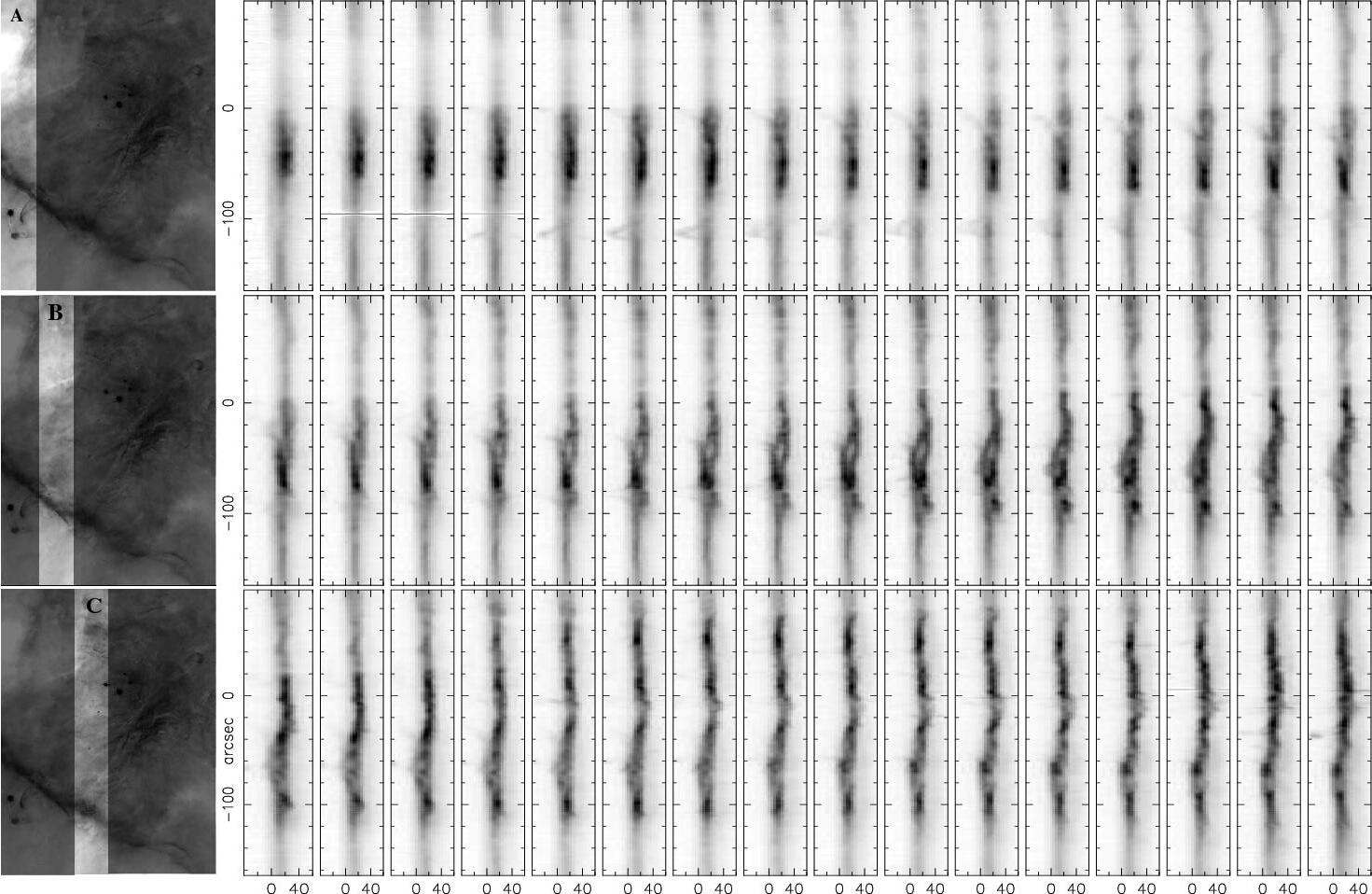
Figure 10: As Figure 1 but for [O 3] 5007 Å.

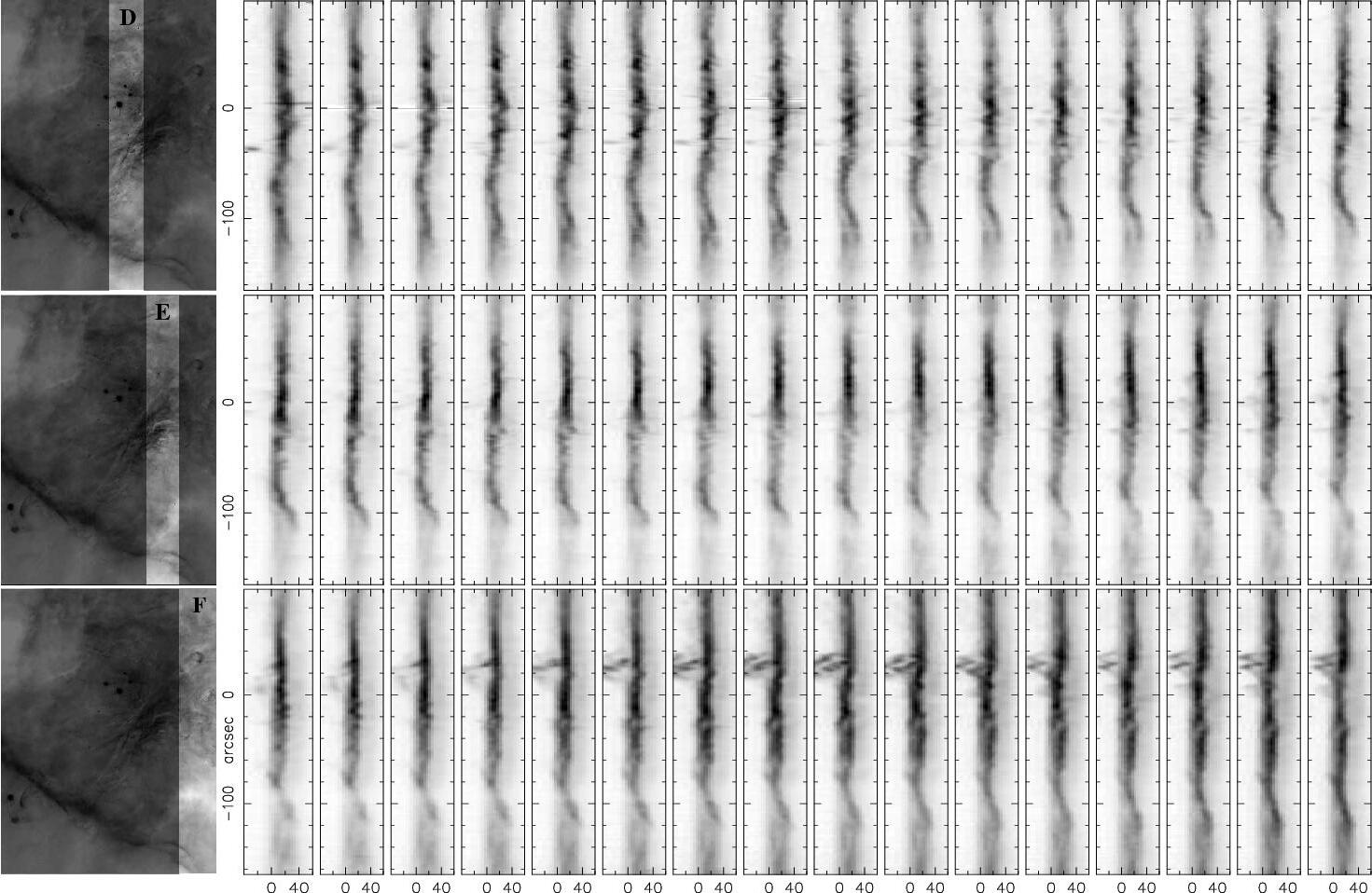
Figure 11: As Figure 1 but for [O 3] 5007 Å, continued.

Table 1: Emission lines in the atlas

	N-S slit positions
Line	KPNO	SPM	Total
[O 1] 6300 Å		60	60
[S 2] 6716,6731 Å	37	55	92
[N 2] 6584 Å	96		96
[S 3] 6312 Å		60	60
$\mathrm{H}\alpha$ 6563 Å	96		96
[O 3] 5007 Å	96		96

The spectral line data used to construct the atlas come from observations at two different observatories, KPNO and SPM. The number of north-south oriented slits from each observatory that contribute to the dataset for each emission line is given in Table 1.

The SPM observations were obtained with the Manchester echelle spectrometer (MES; Meaburn et al., 2003) combined with the f/7.8 focus on the 2.1 m San Pedro Mártir telescope of the Universidad Nacional Autónoma de México, further details of the observations are described in Paper I). The KPNO observations were obtained with the echelle spectrometer attached to the f/8 Cassegrain focus of the Mayall 4 m telescope at Kitt Peak National Observatory, further details are given in O’Dell et al. (2001) and Doi et al. (2004).

The SPM-MES spectra were obtained with a slit width of 150 $\mu$m (2.0) for a resolution of 12 $\mathrm{km\ s}^{-1}$, although a few positions were observed with a narrower, 70 $\mu$m (0.9) slit and a 6 $\mathrm{km\ s}^{-1}$, resolution. The slit length at SPM is 312. For KPNO the slit width is 130 $\mu$m (0.8), the slit length 300 and 8 $\mathrm{km\ s}^{-1}$ resolution. Further details of the data reduction steps are given in DOH04 and Paper I. Since the original analysis of DOH04 was oriented towards fast-moving jets and shocks, the tolerances employed for their velocity calibration ($\simeq 4\leavevmode\nobreak\ \mathrm{km\ s}^{-1}{}$) did not need to be as tight as in DOH04. Furthermore, although Paper I employed an E-W slit in order to tie together the velocity calibrations of the multiple N-S slits, this was not done by DOH04. Instead, it was assumed that the mean velocity, integrated over each slit, was constant as a function of right ascension.

We have therefore internally re-calibrated each DOH04 velocity cube in two ways. First, we have applied small rectification corrections in order to remove obvious discontinuities between adjacent slits, which become apparent when examining the kinematics of slow-moving gas. For $\mathrm{H}\alpha$ and [N 2], the affected slits are all those lying between $x=-55$ and $x=47$, whereas for [O 3] no corrections were necessary. A common velocity correction, which is linear in distance along the slit, is applied to all the affected slits in each emission line: $\delta V=a+by$ ($\delta V$ is in $\mathrm{km\ s}^{-1}$, while $x$ and $y$ are in arcsec with respect to $\theta^{1}$ Ori C), with $a=-0.7$, $b=-0.013$ for $\mathrm{H}\alpha$ and $a=-0.4$, $b=-0.015$ for [N 2]. The velocity corrections to individual pixels vary between $\delta V\simeq-3\leavevmode\nobreak\ \mathrm{km\ s}^{-1}{}$ in the far south to $\delta V\simeq+1\leavevmode\nobreak\ \mathrm{km\ s}^{-1}{}$ in the far north. Although this procedure greatly reduced the discontinuities, it did not remove them completely in the case of $\mathrm{H}\alpha$.

For the second recalibration, in order to correct large-scale trends in the mean velocity as a function of right ascension, we have obtained new observations in February 2007 through an E-W oriented slit, positioned 22S of $\theta^{1}$ Ori C. These observations were obtained with SPM-MES, using a 70 $\mu$m slit and an instrumental configuration identical to that of Paper I, except for the filters employed. The mean velocities of [N 2], $\mathrm{H}\alpha$, and [O 3] were calculated as a function of RA along the slit, and these were compared with the mean velocities extracted from the DOH04 velocity cubes for the same slit. For [N 2], we found an rms difference $<1\leavevmode\nobreak\ \mathrm{km\ s}^{-1}{}$, so no correction was applied. However, for $\mathrm{H}\alpha$ and [O 3], systematic discrepancies of $\sim 5\leavevmode\nobreak\ \mathrm{km\ s}^{-1}{}$ are seen in the west of the nebula. We have therefore fitted a third order polynomial to the velocity differences as a function of RA and used it to correct each slit of the DOH04 cube.

In order to check the calibration of the absolute velocity scale for each emission line, we have compared our results with those from previous studies (Balick et al., 1980; Castañeda, 1988; Wen & O’Dell, 1993; Henney & O’Dell, 1999; Baldwin et al., 2000). In all cases, we found agreement to within $2\leavevmode\nobreak\ \mathrm{km\ s}^{-1}$.

In summary, we estimate that over most of the [S 2], [N 2], $\mathrm{H}\alpha$, and [O 3] maps, the relative velocities of each emission line are accurate to $\sim 0.5\leavevmode\nobreak\ \mathrm{km\ s}^{-1}{}$ over relatively short distances ($<50^{\prime\prime}$) in the declination direction, but only accurate to $\simeq 1\leavevmode\nobreak\ \mathrm{km\ s}^{-1}{}$ when comparing points lying in different slits or widely separated in declination. For the [S 3] and [O 1] lines, the low signal-to-noise ratio over much of the map means that the accuracy is much worse than this for individual spatial pixels, and therefore the same velocity precision can only be retrieved by integrating the line profile over an extended region and thus losing spatial resolution. For the absolute value of the mean velocity of the different lines, we also estimate an uncertainty of $1$–$2\leavevmode\nobreak\ \mathrm{km\ s}^{-1}{}$.

Figures 1–5 show the individual long-slit spectra in the form of calibrated position-velocity (P-V) arrays. The HST image of Orion at the left of the figures shows with a highlighted strip the region covered by the sixteen slit positions shown to the right. The strip advances to the right (west) in the following rows indicating the corresponding regions for the spectra. Figures 1 & 2 correspond to the [S 2] 6731 Å emission line. We do not show here the data for the [S 2] 6716 Å component, although the [S 2] line ratio has been used by Paper I to derive the spatially resolved electron density for the whole region. Strips A–F in Figures 1 and 2 cover the full survey area for [S 2]. Figures 3 and 4 (Strips A–C) correspond to [O 1] 6300 Å and finally Figures 4 (Strip D) and 5 (Strips A–B) correspond to [S 2] 6731 Å.

The spectra are presented within a heliocentric velocity range of $-40$ to $+60\leavevmode\nobreak\ \mathrm{km\ s}^{-1}{}$ in all cases. We choose this range because it allows one to appreciate the complex structure of the nebula at these relatively low velocities, although some high velocity features, as those from HH jets fall outside the range displayed, but still can be clearly identified. The declination scale and right ascension scale set the zero referred with respect to $\theta^{1}$ Ori C. The stellar continua have been subtracted from the spectra. Note that the mean velocities of the background molecular cloud and of the stars in the Orion Nebula Cluster are both $V_{\odot}\simeq 27\pm 2\leavevmode\nobreak\ \mathrm{km\ s}^{-1}$ and that the conversion to “local standard of rest” (LSR) velocities is $V_{\mathrm{LSR}}=V_{\odot}-18.1\leavevmode\nobreak\ \mathrm{km\ s}^{-1}{}$.

0.3 Maps of line profile parameters

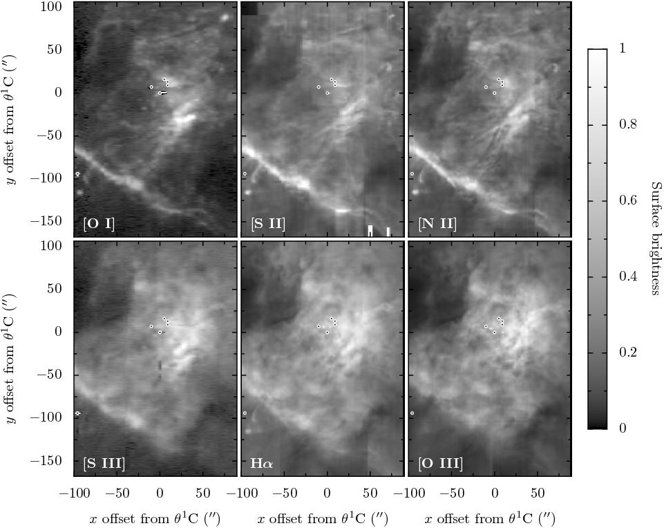
Figure 12: Reconstructed maps of emission line surface brightness, $S$, in the range $V_{\odot}=-40$ to $V_{\odot}=+70\leavevmode\nobreak\ \mathrm{km\ s}^{-1}$.

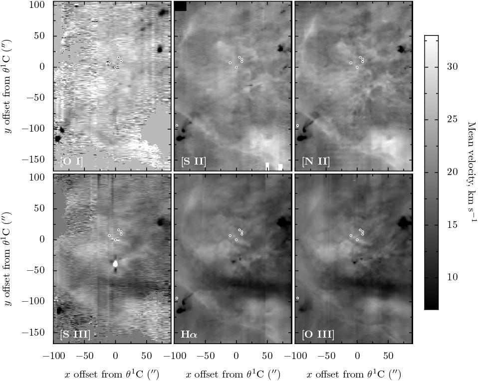
Figure 13: As Fig. 12 but for the mean velocity, $\langle V\rangle$.

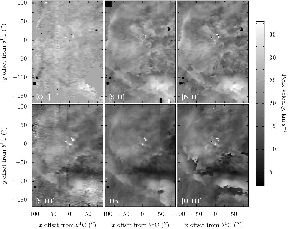
Figure 14: As Fig. 12 but for the peak velocity, $V_{\mathrm{p}}$.

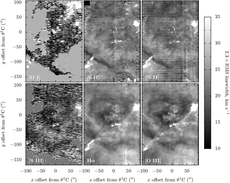
Figure 15: As Fig. 12 but for the instrumentally and thermally corrected rescaled RMS line width, $(8\ln 2)^{1/2}\sigma$.

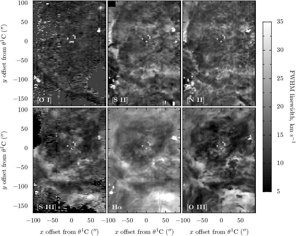
Figure 16: As Fig. 12 but for the instrumentally and thermally corrected FWHM line width, $W$.

In order to provide a global overview of the nebular structure and kinematics, we show in Figures 12 to 16 maps of derived parameters of the line profile of each emission line at each point in the nebula. These offer a complementary approach to the isovelocity channel maps that have already been published (Doi et al., 2004; García-Díaz & Henney, 2007; Henney et al., 2007). The parameters shown are total line surface brightness, $S$, mean velocity, $\langle V\rangle$, root-mean-square (RMS) linewidth, $\sigma$, peak velocity, $V_{\mathrm{p}}$, and full width at half maximum (FWHM) linewidth, $W$. The first three of these quantities can be defined in terms of the first three velocity moments, $M_{k}$, of the line profiles $I(V)$:

$$M_{k}=\int_{V_{1}}^{V_{2}}V^{k}I(V)\,dV,$$ (1)

such that $S=M_{0}$, $\langle V\rangle=M_{1}/M_{0}$, and $\sigma^{2}=(M_{2}/M_{0})-\langle V\rangle^{2}$. The limits of integration are chosen to be $V_{1}=-40\leavevmode\nobreak\ \mathrm{km\ s}^{-1}$ and $V_{2}=+70\leavevmode\nobreak\ \mathrm{km\ s}^{-1}$ for all lines, which represents a compromise between being a wide enough range to include most emission of interest, but not so wide as to introduce too much noise into the maps. This is is a particular issue for $\sigma$, which is very sensitive to noise in the far wings of the $I(V)$ profile. The remaining quantities, $V_{\mathrm{p}}$, and $W$ are directly measured from the line profile. In order to determine $V_{\mathrm{p}}$ to a precision greater than the size of the velocity pixels, we use parabolic interpolation between the peak pixel and its two neighbours. Similarly, $W$ is calculated as the difference between the velocities of two half-power points, which are found from linear interpolation between adjacent pixels. In the case that the profile has more than two half-power points, $W$ is defined as the difference between the highest and lowest of these.

Figure 12 shows the reconstructed surface brightness maps in the six lines. Comparison with published direct imaging (e.g., Pogge et al., 1992) shows generally good agreement, although some artefacts remain from the process of combining the individual spectra. These can easily be identified as brightness discontinuities across vertical lines in the maps. The most serious of these artefacts are in the [S 2] map at $x=+10$, $x=+45$, in the [N 2] and $\mathrm{H}\alpha$ maps at $x=+45$, in the [S 3] map at $x=0$, and in the [O 3] map at $x=-5$.

The mean and peak velocities are shown in Figures 13 and 14, where it can be seen that the two quantities are generally well-correlated for a given line, although there are some important differences. The mean velocity varies smoothly across the face of the nebula, whereas the peak velocity shows frequent discontinuities, which are caused by one particular line component becoming brighter than another. The mean velocity is also more sensitive to high velocity components, such as HH objects. This is particularly notable in the case of [O 3], where the HH objects do not show up at all in the $V_{\mathrm{p}}$ image. Since [S 3] and [O 1] are very much weaker than the other lines, the velocity maps are rather noisy, especially in the faint regions of the nebula. We have therefore masked out from the velocity maps all regions with a surface brightness below a certain threshold, which appear as solid gray areas in the figures.

The non-thermal contributions to the RMS and FWHM line widths are shown in Figure 15 and 16. These are calculated by subtracting in quadrature the instrumental and thermal widths from the raw measured widths, assuming a gas temperature of $9100$ K (see § 0.5). For a Gaussian profile, the relationship between the FWHM and RMS widths is $W=(8\ln 2)^{1/2}\sigma\simeq 2.355\sigma$. We therefore multiply the values of $\sigma$ by 2.355 to allow direct comparison between the $\sigma$ and $W$ maps. There is generally a much greater difference between the $\sigma$ and $W$ maps of a given line than between the maps of $\langle V\rangle$ and $V_{\mathrm{p}}$. The $\sigma$ maps are very much dominated by high-velocity flows, which are much less apparent in the $W$ maps. As with the $V_{\mathrm{p}}$ maps, the $W$ maps show discontinuities between patches of the nebula with high and low line widths. An exception is the $\mathrm{H}\alpha$ line, where the increased thermal broadening leads to a more Gaussian-like line profile and a closer resemblance between the $W$ and $\sigma$ maps. As with the velocity maps, we have masked out regions of low signal-to-noise ratio for the [O 1] and [S 3] lines.

An empirical description of the nebular structure and kinematics was given in § 3 of Paper I and will not be repeated here. The reader is referred in particular to Fig. 7 of Paper I for orientation in identifying nebular features mentioned in the remainder of the paper.

0.4 One-point velocity statistics

Table 2: Summary of velocity statistics

line	$\langle V\rangle$	$V_{\mathrm{p}}$	$\sigma^{2}$	$W$
$[{O\textsc{3}}]$	$16.3\pm 2.8$	$15.5\pm 4.0$	$113\pm 29$	$14.7\pm 5.1$
$\mathrm{H}\alpha$	$16.8\pm 3.0$	$16.2\pm 4.1$	$195\pm 28$	$18.6\pm 5.1$
$[{S\textsc{3}}]$	$19.7\pm 3.0$	$19.2\pm 4.0$	$99\pm 46$	$14.6\pm 4.4$
$[{N\textsc{2}}]$	$20.5\pm 2.9$	$21.1\pm 3.7$	$106\pm 24$	$15.4\pm 3.7$
$[{S\textsc{2}}]$	$21.2\pm 2.4$	$21.8\pm 3.2$	$114\pm 21$	$15.2\pm 3.5$
$[{O\textsc{1}}]$	$25.7\pm 3.4$	$26.3\pm 2.5$	$106\pm 65$	$11.5\pm 2.6$
$\mathrm{H}\alpha-[{O\textsc{3}}]$	$0.5\pm 1.4$	$0.7\pm 3.2$	$82.2\pm 11.8$	$3.9\pm 3.0$
$r$	$0.889$	$0.700$	$0.917$	$0.825$
$[{N\textsc{2}}]-[{O\textsc{3}}]$	$4.2\pm 2.8$	$5.6\pm 4.5$	$-7.0\pm 36.8$	$0.7\pm 6.5$
$r$	$0.511$	$0.274$	$0.287$	$-0.067$
$[{S\textsc{2}}]-[{S\textsc{3}}]$	$1.6\pm 2.5$	$2.6\pm 3.3$	$18.0\pm 46.8$	$0.2\pm 5.6$
$r$	$0.617$	$0.588$	$0.229$	$0.065$
$[{O\textsc{1}}]-[{S\textsc{2}}]$	$4.4\pm 3.0$	$4.5\pm 2.7$	$-7.6\pm 64.8$	$-3.7\pm 4.2$
$r$	$0.507$	$0.580$	$0.175$	$0.078$

(a)

(b)

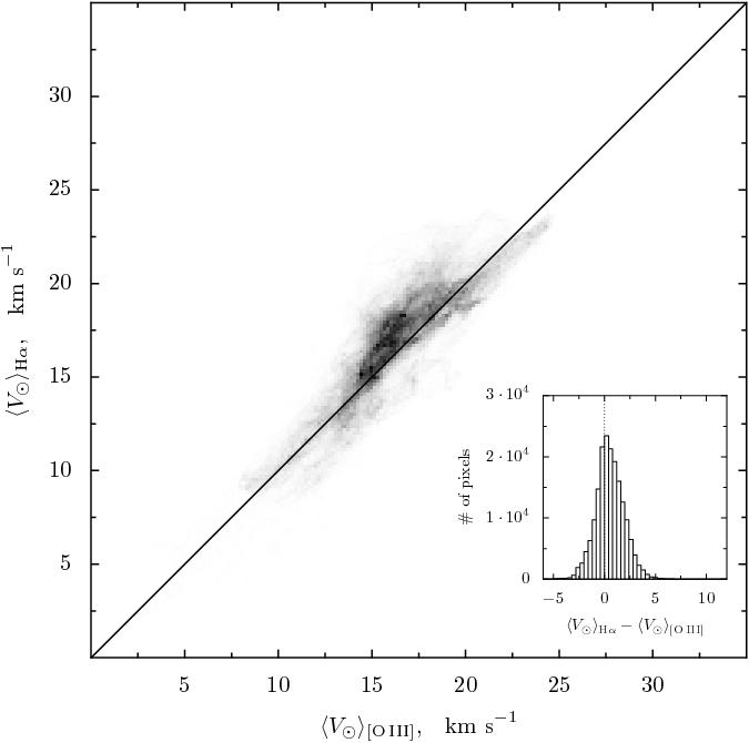
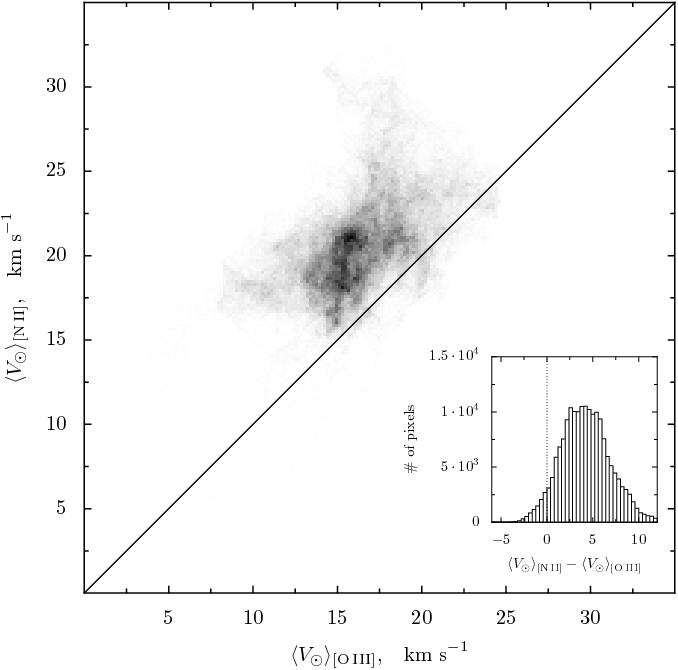
(c)

(d)

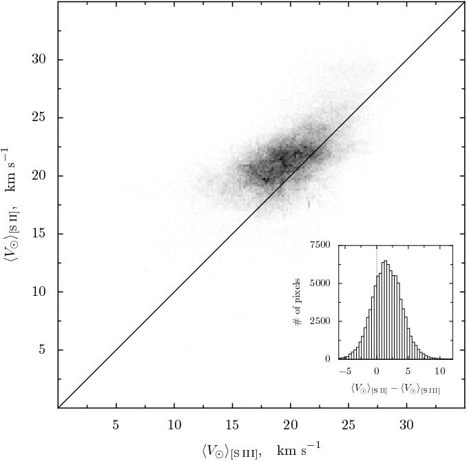
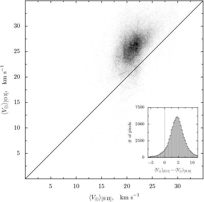
Figure 17: Joint distribution of mean velocities, $\langle V\rangle$, of different emission lines, with inset box showing a histogram of differences in $\langle V\rangle$. In each case, the straight line shows the case of equal velocities in the two lines. (a) $\langle V\rangle_{\mathrm{H}\alpha}$ versus $\langle V\rangle_{\mathrm{[\mathrm{O\,III}]}}$. (b) $\langle V\rangle_{\mathrm{[\mathrm{N\,II}]}}$ versus $\langle V\rangle_{\mathrm{[\mathrm{O\,III}]}}$ (c) $\langle V\rangle_{\mathrm{[\mathrm{S\,II}]}}$ versus $\langle V\rangle_{\mathrm{[\mathrm{S\,III}]}}$. (d) $\langle V\rangle_{\mathrm{[\mathrm{O\,I}]}}$ versus $\langle V\rangle_{\mathrm{[\mathrm{S\,II}]}}$

(a)

(b)

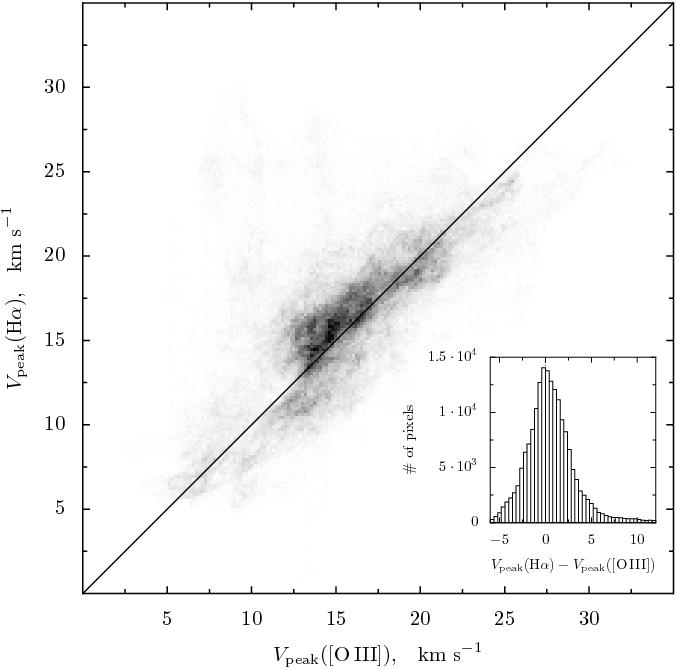
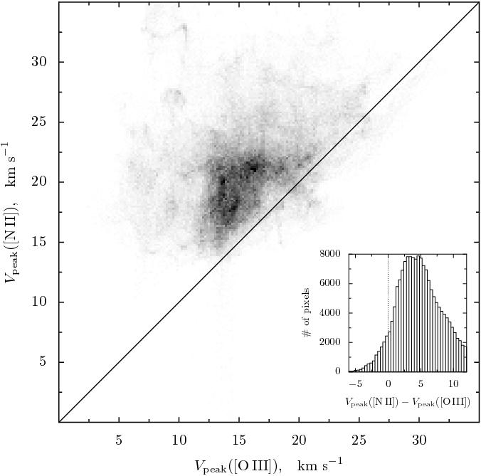
(c)

(d)

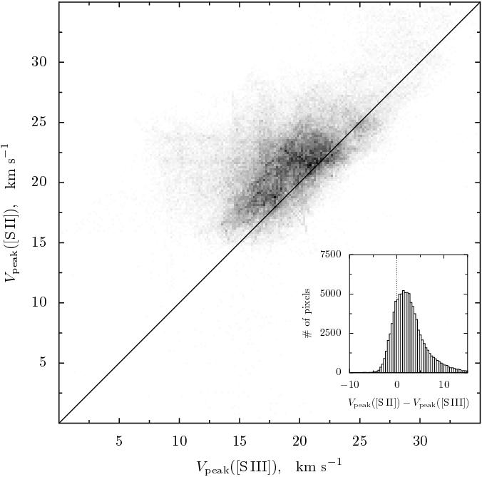
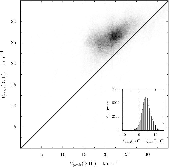
Figure 18: Joint distribution of peak velocities, $V_{\mathrm{p}}$, of different emission lines, with inset box showing a histogram of differences in $V_{\mathrm{p}}$. In each case, the straight line shows the case of equal velocities in the two lines. (a) $V_{\mathrm{p}}({\mathrm{H}\alpha})$ versus $V_{\mathrm{p}}({\mathrm{[\mathrm{O\,III}]}})$. (b) $V_{\mathrm{p}}({\mathrm{[\mathrm{N\,II}]}})$ versus $V_{\mathrm{p}}({\mathrm{[\mathrm{O\,III}]}})$ (c) $V_{\mathrm{p}}({\mathrm{[\mathrm{S\,II}]}})$ versus $V_{\mathrm{p}}({\mathrm{[\mathrm{S\,III}]}})$. (d) $V_{\mathrm{p}}({\mathrm{[\mathrm{O\,I}]}})$ versus $V_{\mathrm{p}}({\mathrm{[\mathrm{S\,II}]}})$

(a)

(b)

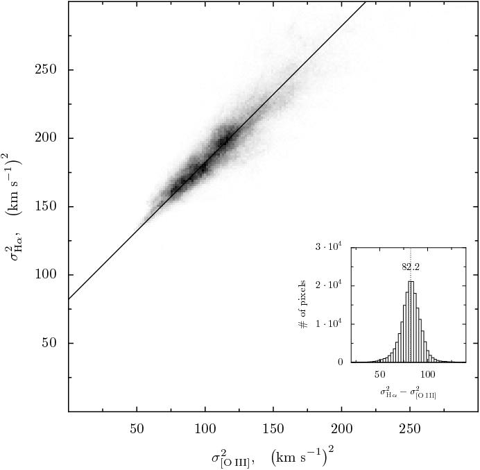
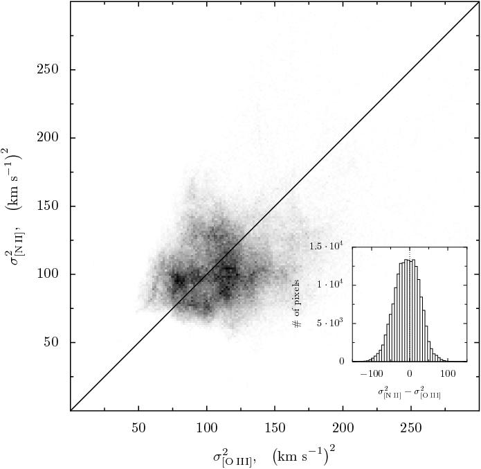
(c)

(d)

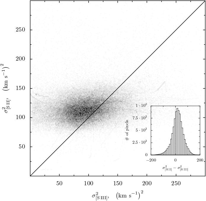
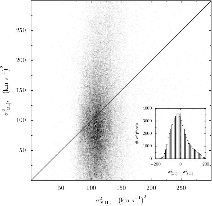
Figure 19: Joint distribution of raw measured mean square velocity widths, $\sigma^{2}$, of different emission lines, with inset box showing a histogram of the differences in $\sigma^{2}$. (a) $\sigma^{2}_{\mathrm{H}\alpha}$ versus $\sigma^{2}_{\mathrm{[\mathrm{O\,III}]}}$. (b) $\sigma^{2}_{\mathrm{[\mathrm{N\,II}]}}$ versus $\sigma^{2}_{\mathrm{[\mathrm{O\,III}]}}$. (c) $\sigma^{2}_{\mathrm{[\mathrm{S\,II}]}}$ versus $\sigma^{2}_{\mathrm{[\mathrm{S\,III}]}}$. (d) $\sigma^{2}_{\mathrm{[\mathrm{O\,I}]}}$ versus $\sigma^{2}_{\mathrm{[\mathrm{S\,II}]}}$. The diagonal straight line in each panel shows the case of equal variances in the two lines, except for in panel a, where it shows the relation $\sigma^{2}_{\mathrm{H}\alpha}=\sigma^{2}_{\mathrm{[\mathrm{O\,III}]}}+82.2$.

(a)

(b)

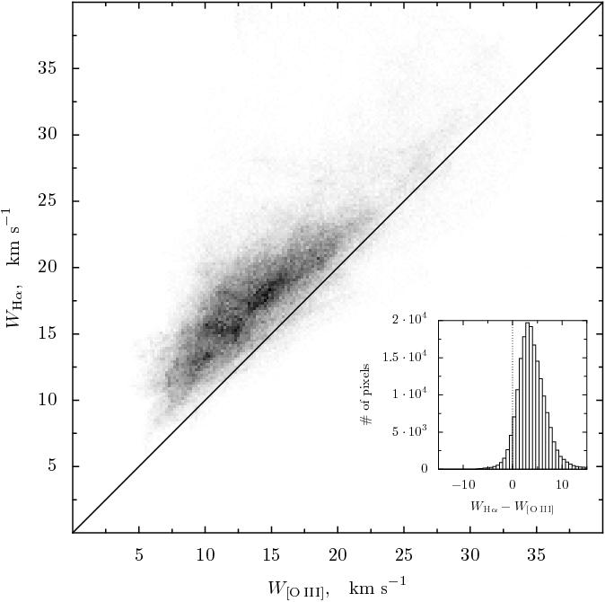
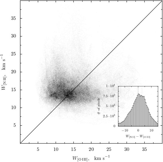
(c)

(d)

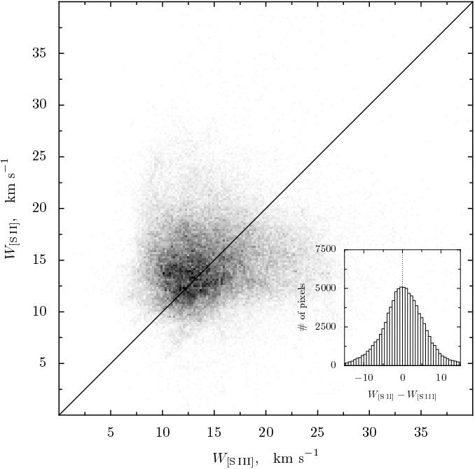
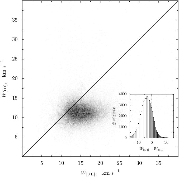
Figure 20: Joint distribution of corrected full-widths at half maximum, $W$, of different emission lines, with inset box showing a histogram of differences in $W$. The thermal and instrumental widths have been subtracted in quadrature from the raw measured values. In each case, the straight line shows the case of equal widths in the two lines. (a) $W_{\mathrm{H}\alpha}$ versus $W_{\mathrm{[\mathrm{O\,III}]}}$. (b) $W_{\mathrm{[\mathrm{N\,II}]}}$ versus $W_{\mathrm{[\mathrm{O\,III}]}}$ (c) $W_{\mathrm{[\mathrm{S\,II}]}}$ versus $W_{\mathrm{[\mathrm{S\,III}]}}$. (d) $W_{\mathrm{[\mathrm{O\,I}]}}$ versus $W_{\mathrm{[\mathrm{S\,II}]}}$

In Figures 17 and 18 we show joint distributions of the mean and peak velocities, respectively, for selected pairs of emission lines, which illustrate the correlations that exist between the kinematics of the different emission zones of the nebula. Figure 19 shows the joint distributions of the raw velocity variance, $\sigma^{2}$, which is the square of the RMS velocity dispersion, and Figure 20 shows distributions of the non-thermal FWHM linewidth, $W$. The values of $W$ have been approximately corrected for thermal, instrumental and fine-structure broadening in the same way as in Figure 16, whereas the values of $\sigma^{2}$ in Figure 19 are uncorrected and measured directly from the data.

The statistics for individual lines are summarised in the upper part of Table 2, which shows the mean and standard deviation (s.d.) of each quantity. These are calculated with an equal weighting of each pixel in the map after masking out any points lying outside the ranges shown in Figures 17–20. For [S 3] and [O 1], any pixel with surface brightness below the thresholds shown in Figures 13–16 were also masked out. The lower part of Table 2 show the mean and s.d. of the differences between the kinematic quantities for the line pairs shown in the figures, together with the linear correlation coefficient, $r$, of the joint distributions. In cases where the quantities are well correlated ($r\gtrsim 0.5$), the s.d. of the difference can be significantly less than the s.d.’s of the individual values.

The general trend of increasing blueshifts with increasing degree of ionization is readily apparent from the table, which is arranged from highest to lowest ionization. The mean and peak velocities always show a positive correlation between different lines. The correlation is highest ($r\simeq 0.9$) between H$\alpha$ and [O 3], which is not surprising since there is a large overlap of the emission zones of these two lines. However, even pairs of lines that should not greatly overlap (such as $[{N\textsc{2}}]{}-[{O\textsc{3}}]{}$ and $[{S\textsc{2}}]{}-[{S\textsc{3}}]{}$) also show significant correlation ($r>0.5$).

The s.d. of 1.4 $\mathrm{km\ s}^{-1}$ for $\langle V\rangle_{\mathrm{H}\alpha}-\langle V\rangle_{\mathrm{[\mathrm{O\,III}]}}$ is a hard upper limit on the uncorrelated average wavelength calibration errors within the individual lines. Given that $\langle V\rangle_{\mathrm{[\mathrm{N\,II}]}}-\langle V\rangle_{\mathrm{[\mathrm{O\,III}]}}$ has a much larger s.d. (2.8 $\mathrm{km\ s}^{-1}$) and that some fraction of the $\mathrm{H}\alpha$ emission comes from the [N 2] zone, it follows that at least some of the scatter in $\langle V\rangle_{\mathrm{H}\alpha}-\langle V\rangle_{\mathrm{[\mathrm{O\,III}]}}$ must be real. This is consistent with our estimate above in § 0.2 that the relative velocity calibration within each emission line is good to $\simeq 1\leavevmode\nobreak\ \mathrm{km\ s}^{-1}{}$. Our worst-case estimate for the uncertainty in the absolute velocity calibration for each line is 2 $\mathrm{km\ s}^{-1}$ and this translates into uncertainties in the average values of the differences in mean and peak velocities. This issue is returned to in § 0.5 below, where we argue that the absolute velocity calibration must be better than this conservative estimate.

An extremely tight correlation ($r\simeq 0.9$) is seen between the mean square velocity widths of H$\alpha$ and [O 3], whereas no other pair of lines show a significant correlation in this quantity. The large offset $\bigl{\langle}\sigma^{2}_{\mathrm{H}\alpha}-\sigma^{2}_{\mathrm{[\mathrm{O\,III}]}}\bigr{\rangle}=(82.2\pm 18.2)\leavevmode\nobreak\ \mathrm{km^{2}\ s}^{-2}$ is due mainly to the extra thermal broadening of $\mathrm{H}\alpha$, as is discussed further in § 0.5 below. Other pairs of lines show much smaller offsets in $\sigma^{2}$, with no obvious trends with ionization. The s.d. of $\sigma^{2}$ is very large in the case of [O 1] and [S 3] because of the low signal-noise ratio of these weak lines.

A similar picture is seen for the corrected full width half maxima, $W$: only in the case of $\mathrm{H}\alpha{}-[{O\textsc{3}}]{}$ does a correlation exist. Note that even though the effects of thermal and fine structure broadening have been subtracted in quadrature to obtain $W$, a residual difference remains between $\mathrm{H}\alpha$ and [O 3] of $\simeq 4\leavevmode\nobreak\ \mathrm{km\ s}^{-1}$. We believe that this is because the FWHM is such a mathematically ill-behaved quantity that quadrature subtraction cannot be expected to work reliably in the presence of strongly non-Gaussian lineshapes. For example, consider a line that consists of two components, A and B, separated by $\delta v$ and each of width $w$, where the intensity of B is less than half that of A. The measured FWHM will not be affected at all by the presence of component B unless the components are blended: $\delta v\lesssim w$. The larger thermal broadening of $\mathrm{H}\alpha$ gives a larger $w$, so that there will be cases where the FWHM of $\mathrm{H}\alpha$ can “see” component B, but the FWHM of [O 3] cannot. Evidence for this can be seen in Figure 16, where the [O 3] map shows multiple dark patches of low FWHM, which are absent from the $\mathrm{H}\alpha$ map.

All the metal lines show very similar mean values of $\langle W\rangle\simeq 15\leavevmode\nobreak\ \mathrm{km\ s}^{-1}{}$, except for [O 1], which is significantly lower, $\langle W\rangle\simeq 12\leavevmode\nobreak\ \mathrm{km\ s}^{-1}{}$. The FWHM is affected by noise to a much smaller extent than $\sigma^{2}$ and the metal lines all have low thermal widths, so should not be affected by the problem discussed in the previous paragraph.

0.5 Derivation of the mean electron temperature from linewidths

In this section, we use the statistics of the observed line profiles of [N 2], $\mathrm{H}\alpha$, and [O 3] (§ 0.4) to derive the mean electron temperature in the nebula and to show that the “non-thermal” component to the line broadening is not significantly larger in $\mathrm{H}\alpha$ than in the metal lines. The method we employ is essentially an old one (Courtès et al., 1968; Dyson & Meaburn, 1971), which estimates the gas temperature by comparing the width of a metal line with that of a hydrogen line, under the assumption that the excess width of the hydrogen line is principally due to its greater thermal broadening on account of its lower atomic weight. A problem with many applications of this method has been that the metal line and hydrogen line (usually [N 2] and $\mathrm{H}\alpha$) are not necessarily emitted by the same volume of gas. Indeed, previous applications of this method to the Orion nebula (Dopita et al., 1973; Gibbons, 1976) have shown that the $\mathrm{H}\beta$-[O 3] pair gives results that are very different from the $\mathrm{H}\alpha$-[N 2] pair and that are seemingly more reliable. Our own version of the method improves on previous versions by using all three emission lines [N 2], $\mathrm{H}\alpha$, and [O 3] in order to control for the imperfect overlap of the emission regions.

0.5.1 Components of the observed line widths

For each emission line, the observed mean square velocity width at a certain point on the nebula can be broken down schematically into four components:

$$\sigma^{2}=\sigma^{2}_{\mathrm{th}}+\sigma^{2}_{\mathrm{fs}}+\sigma^{2}_{\mathrm{ins}}+\sigma^{2}_{\mathrm{nt}}.$$ (2)

The first term in this equation is the thermal Doppler width, $\sigma^{2}_{\mathrm{th}}=82.5(T_{4}/A)$ $\mathrm{km^{2}\ s}^{-2}$, where $T_{4}=T/10^{4}\leavevmode\nobreak\ \mathrm{K}$ and $A$ is the atomic weight of the atom or ion. The second term is the fine structure broadening, which is important for hydrogen and helium recombination lines, but not for metal lines such as [O 3] and [N 2]. In Appendix 0.9, we show that its value for $\mathrm{H}\alpha$ is $\sigma^{2}_{\mathrm{fs}}=10.233\leavevmode\nobreak\ \mathrm{km^{2}\ s}^{-2}$. The third term is the instrumental width, which for the KPNO observations is approximately $\sigma^{2}_{\mathrm{ins}}=11.5\leavevmode\nobreak\ \mathrm{km^{2}\ s}^{-2}$, and which is the same for the three lines. The fourth term, $\sigma^{2}_{\mathrm{nt}}$, is the “non-thermal” contribution, which is a catch-all term for any other broadening process. This might include Doppler broadening due to velocity gradients or turbulence within the emitting regions, broadening due to scattering by dust particles, or any other process.

Applying the above equation to differences in $\sigma^{2}$ measured in § 0.4 gives

$$\sigma^{2}_{\mathrm{H}\alpha}-\sigma^{2}_{\mathrm{[\mathrm{O\,III}]}}=77.34T_{4}+10.233\\ +\sigma^{2}_{\mathrm{nt,\mathrm{H}\alpha}}-\sigma^{2}_{\mathrm{nt,\mathrm{[\mathrm{O\,III}]}}}$$ (3)

and

$$\sigma^{2}_{\mathrm{[\mathrm{N\,II}]}}-\sigma^{2}_{\mathrm{[\mathrm{O\,III}]}}=0.74T_{4}+\sigma^{2}_{\mathrm{nt,\mathrm{[\mathrm{N\,II}]}}}-\sigma^{2}_{\mathrm{nt,\mathrm{[\mathrm{O\,III}]}}}.$$ (4)

Note that the instrumental contribution cancels from these equations. The simplest way of extracting the temperature, and what has been done in the past, is then to assume that the difference in non-thermal widths is negligible, so that $T_{4}$ can be calculated directly from the measured $\sigma^{2}_{\mathrm{H}\alpha}-\sigma^{2}_{\mathrm{[\mathrm{O\,III}]}}$ as

$$T^{\prime}_{4}=\bigl{(}\sigma^{2}_{\mathrm{H}\alpha}-\sigma^{2}_{\mathrm{[\mathrm{O\,III}]}}-10.233\bigr{)}/77.34$$ (5)

However, by including the data on the [N 2] line, it is possible to derive a lower bound on the value of $\sigma^{2}_{\mathrm{nt,\mathrm{H}\alpha}}-\sigma^{2}_{\mathrm{nt,\mathrm{[\mathrm{O\,III}]}}}$ and so arrive at a more reliable temperature determination than the naive estimate $T^{\prime}_{4}$.

0.5.2 Correction for differences in temperature and non-thermal widths between high and low ionization zones

We adopt a simplified two-zone model for the emission structure along a given line of sight through the nebula. The first zone, A, contributes all the [O 3] emission plus a fraction, $f$, of the $\mathrm{H}\alpha$ emission. The second zone, B, contributes all the [N 2] emission plus the remaining fraction, $1-f$, of the $\mathrm{H}\alpha$ emission. We further assume that the non-thermal broadening is the same for all emission lines that arise from the same volume (this assumption should hold true for turbulent or other kinematic broadening, an issue we will return to later). A fundamental property of the moments of the line profile given in equation (1) is that they are all additive, with consequences that are elucidated in Appendix 0.8. From equation (9) it follows that

$$\sigma^{2}_{\mathrm{nt,\mathrm{H}\alpha}}-\sigma^{2}_{\mathrm{nt,\mathrm{[\mathrm{O\,III}]}}}=(1-f)(\sigma^{2}_{\mathrm{nt,\mathrm{[\mathrm{N\,II}]}}}-\sigma^{2}_{\mathrm{nt,\mathrm{[\mathrm{O\,III}]}}})\\ +f(1-f)\bigl{(}\langle V\rangle_{\mathrm{[\mathrm{N\,II}]}}-\langle V\rangle_{\mathrm{[\mathrm{O\,III}]}}\bigr{)}^{2}.$$ (6)

Note that the above equation is only valid if the effects of dust extinction are the same for zones A and B, but this is probably a good approximation since O’Dell & Yusef-Zadeh (2000) showed that the majority of the dust extinction in Orion arises in the neutral veil, in the foreground of the ionized gas.

We also allow the two emission zones to have different temperatures, $T_{\mathrm{A}}$ and $T_{\mathrm{B}}$, such that the mean $\mathrm{H}\alpha$ temperature is $T=fT_{\mathrm{A}}+(1-f)T_{\mathrm{B}}$. We can now combine equation (6) with equations (3) and (4), modified to account for the temperature difference between the zones, to obtain

$$T_{4}=\eta T^{\prime}_{4}+\epsilon-\zeta-\xi,$$ (7)

where

$$\eta=\bigl{(}1-0.00957\,(1-f)\bigr{)}^{-1},$$ (8)

$$\epsilon=0.00957\,\eta\,f(1-f)\bigl{(}T_{\mathrm{B}}-T_{\mathrm{A}}\bigr{)}/10^{4}\leavevmode\nobreak\ \mathrm{K},$$ (9)

$$\zeta=0.01293\,\eta\,(1-f)\bigl{(}\sigma^{2}_{\mathrm{[\mathrm{N\,II}]}}-\sigma^{2}_{\mathrm{[\mathrm{O\,III}]}}\bigr{)},$$ (10)

$$\xi=0.01293\,\eta\,f(1-f)\bigl{(}\langle V\rangle_{\mathrm{[\mathrm{N\,II}]}}-\langle V\rangle_{\mathrm{[\mathrm{O\,III}]}}\bigr{)}^{2}.$$ (11)

0.5.3 Techniques for estimating the ionization factor $f$

Equation (7) gives the temperature at any point in the nebula in terms of observable quantities and the factor $f$, which can be estimated in two ways: from surface brightness ratios, or from ratios of differences in mean velocity. We shall describe each of these techniques in turn.

We define for each emission line a per-zone mean effective emission coefficient, $\beta$, with units $\mathrm{erg\ cm^{3}\ s^{-1}\ sr^{-1}}$, such that the intrinsic surface brightness of a zone is $S=\beta E$, where $E=\int n_{\mathrm{p}}n_{\mathrm{e}}\,dz$ is the emission measure of the zone. Since [N 2] 6584 Å and $\mathrm{H}\alpha$ 6563 Å are so close in wavelength, they are both affected in the same way by dust extinction, so the observed ratio of their surface brightnesses is equal to the intrinsic value. Therefore, given that [N 2] by construction arises only in Zone B, we have

$$R_{\mathrm{[\mathrm{N\,II}]}}\equiv\frac{S([{N\textsc{2}}])}{S(\mathrm{H}\alpha)}=\frac{\beta_{\mathrm{B}}([{N\textsc{2}}])\,E_{\mathrm{B}}}{\beta_{\mathrm{A}}(\mathrm{H}\alpha)\,E_{\mathrm{A}}+\beta_{\mathrm{B}}(\mathrm{H}\alpha)\,E_{\mathrm{B}}}\\ =(1-f)\frac{\beta_{\mathrm{B}}([{N\textsc{2}}])}{\beta_{\mathrm{B}}(\mathrm{H}\alpha)},$$ (12)

where the last equality follows from the definition of $f$. Hence, if the emission coefficients $\beta_{\mathrm{B}}([{N\textsc{2}}])$ and $\beta_{\mathrm{B}}(\mathrm{H}\alpha)$ are known, then $f$ can be calculated from the observed surface brightness ratio as $f=1-R_{\mathrm{[\mathrm{N\,II}]}}\beta_{\mathrm{B}}(\mathrm{H}\alpha)/\beta_{\mathrm{B}}([{N\textsc{2}}])$. To make use of this equation, it is first necessary to photometrically calibrate the surface brightness maps and we have done this by comparison with published spectrophotometry of the region (Pogge et al., 1992; Baldwin et al., 2000; O’Dell et al., 2003). It is then necessary to estimate the ratio of emission coefficients for conditions typical of Zone B: $T\simeq 10^{4}$ K, $n_{\mathrm{e}}\simeq 5000$, which we have done using the Cloudy plasma code (Ferland, 2000), assuming an N/H abundance ratio of $6\times 10^{-5}$, finding that the ratio is roughly unity. This is consistent with the N⁺/N abundance found by Esteban et al. (1998).

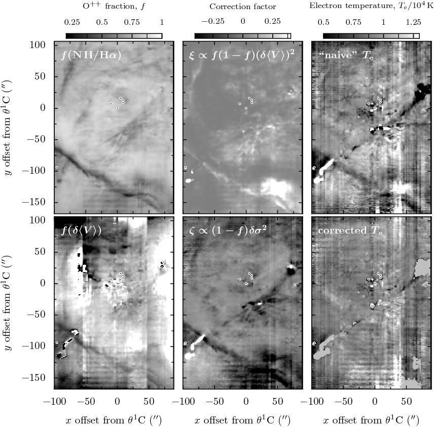
Figure 21: Steps in the construction of the temperature map. Left column: Two independent estimates of the fraction, $f$, of the $\mathrm{H}\alpha$ emission that comes from the O⁺⁺ zone: from the $[{N\textsc{2}}]/\mathrm{H}\alpha$ surface brightness ratio (upper panel), and from the differences in mean velocities of [N 2], $\mathrm{H}\alpha$, [O 3] (lower panel). Center column: Correction factors to the “naive” temperature map due to differences in the kinematics between the N⁺ and O⁺⁺ zones: mean velocity differences, $\xi$ (upper panel) and velocity dispersion differences, $\zeta$ (lower panel). Right column: “naive” temperature estimate (upper panel) from the difference in velocity dispersion of [O 3] and $\mathrm{H}\alpha$ and final corrected temperature estimate (lower panel). The horizontal bands and vertical streaks seen in some panels are instrumental artifacts.

Assuming that $\beta_{\mathrm{B}}(\mathrm{H}\alpha)/\beta_{\mathrm{B}}([{N\textsc{2}}])=1$, we find a mean value of $\langle f\rangle=0.76$ for the entire area covered by our observations. The upper-left panel of Figure 21 shows the map of $f$ calculated by this technique, which varies between 0.26 and 0.91. In reality, $\beta_{\mathrm{B}}(\mathrm{H}\alpha)/\beta_{\mathrm{B}}([{N\textsc{2}}])$ will vary with position due to variations in electron density ([N 2] is affected by collisional deexcitation but $\mathrm{H}\alpha$ is not). A better way of calculating $f$ would be to use the $[{O\textsc{3}}]/\mathrm{H}\beta$ surface brightness ratio, since the critical density for [O 3] is higher than that typically found in the nebula (similar arguments to those above give $f=R_{\mathrm{[\mathrm{O\,III}]}}\beta_{\mathrm{A}}(\mathrm{H}\beta)/\beta_{\mathrm{A}}([{O\textsc{3}}])$, where $R_{\mathrm{[\mathrm{O\,III}]}}=S([{O\textsc{3}}])/S(\mathrm{H}\beta)$). However, our dataset does not include $\mathrm{H}\beta$ and the $[{O\textsc{3}}]/\mathrm{H}\alpha$ ratio would have to be corrected for the highly variable foreground extinction (O’Dell & Yusef-Zadeh, 2000). A comparison of the $[{N\textsc{2}}]/\mathrm{H}\alpha$ and $[{O\textsc{3}}]/\mathrm{H}\beta$ ratios over a limited area (using data from Figs. 11 and 12 of O’Dell et al., 2003) gives an rms scatter of $\pm 0.05$ between the values of $f$ derived from the $R_{\mathrm{[\mathrm{N\,II}]}}$ and $R_{\mathrm{[\mathrm{O\,III}]}}$ techniques, which is roughly half of the total rms variation in $f$ from our maps. The $R_{\mathrm{[\mathrm{O\,III}]}}$-derived values of $f$ have a greater range than the $R_{\mathrm{[\mathrm{N\,II}]}}$-derived values. This is to be expected since, all else being equal, higher density regions will have lower ionization.

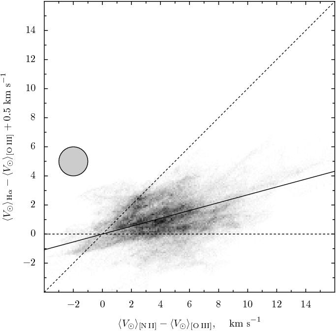
Figure 22: Joint distribution of differences in mean velocities: $\langle V\rangle_{\mathrm{H}\alpha}-\langle V\rangle_{\mathrm{[\mathrm{O\,III}]}}$ versus $\langle V\rangle_{\mathrm{[\mathrm{N\,II}]}}-\langle V\rangle_{\mathrm{[\mathrm{O\,III}]}}$. The values of $\langle V\rangle_{\mathrm{H}\alpha}-\langle V\rangle_{\mathrm{[\mathrm{O\,III}]}}$ have been shifted by 0.5 $\mathrm{km\ s}^{-1}$ so as to make the distribution symmetric about a line through the origin (see discusion in text). The dashed lines show the boundaries of the two triangular regions (upper right and lower left) that give physically possible values of $f$ in the two-zone model. The solid line shows the relationship $\langle V\rangle_{\mathrm{H}\alpha}-\langle V\rangle_{\mathrm{[\mathrm{O\,III}]}}=(1-\langle f\rangle)(\langle V\rangle_{\mathrm{[\mathrm{N\,II}]}}-\langle V\rangle_{\mathrm{[\mathrm{O\,III}]}})$, where $\langle f\rangle$ is determined from the $R_{\mathrm{[\mathrm{N\,II}]}}$ method. The solid gray circle indicates the effect of $\pm 1\leavevmode\nobreak\ \mathrm{km\ s}^{-1}$ uncertainties in the velocities.

A completely independent way of estimating $f$, and one that does not depend on knowing the emission coefficients, is to use the observed mean velocities of the three lines. A corollary of the additive property of the line profile velocity moments (Appendix 0.8) is that in the two-zone model we have from equation (8) that

$$\langle V\rangle_{\mathrm{H}\alpha}=f\langle V\rangle_{\mathrm{[\mathrm{O\,III}]}}+(1-f)\langle V\rangle_{\mathrm{[\mathrm{N\,II}]}},$$ (13)

so that $f$ can be estimated as

$$f=1-\frac{\langle V\rangle_{\mathrm{H}\alpha}-\langle V\rangle_{\mathrm{[\mathrm{O\,III}]}}}{\langle V\rangle_{\mathrm{[\mathrm{N\,II}]}}-\langle V\rangle_{\mathrm{[\mathrm{O\,III}]}}}.$$ (14)

Despite its advantages over the surface brightness method, this technique has two serious limitations. First, equation (14) has a singularity when $\langle V\rangle_{\mathrm{[\mathrm{N\,II}]}}=\langle V\rangle_{\mathrm{[\mathrm{O\,III}]}}$. If the two-zone model were strictly valid, then any pixel with $\langle V\rangle_{\mathrm{[\mathrm{N\,II}]}}=\langle V\rangle_{\mathrm{[\mathrm{O\,III}]}}$ would also have $\langle V\rangle_{\mathrm{H}\alpha}=\langle V\rangle_{\mathrm{[\mathrm{O\,III}]}}$, so the singularity would be benign. However, in reality the two-zone model is only an approximation and, additionally, the observed values of $\langle V\rangle$ will always include a certain measurement error. As a result, applying equation (14) to real data will inevitably result in discontinuities in the $f$ map and unphysical values ($f<0$ or $f>1$) for some pixels. Second, the observed values of $\langle V\rangle_{\mathrm{H}\alpha}-\langle V\rangle_{\mathrm{[\mathrm{O\,III}]}}$ are rather small (typically $-2$ to $+3$ $\mathrm{km\ s}^{-1}$, see Fig. 17a), and are of the same order as the systematic uncertainties in the wavelength calibration.

Given these caveats, it is perhaps surprising that this method works at all. However, the average slope of the relationship between $\langle V\rangle_{\mathrm{H}\alpha}-\langle V\rangle_{\mathrm{[\mathrm{O\,III}]}}$ and $\langle V\rangle_{\mathrm{[\mathrm{N\,II}]}}-\langle V\rangle_{\mathrm{[\mathrm{O\,III}]}}$ should be independent of any inaccuracies in the absolute velocity scales of the individual lines, and by equation (14) should be equal to $1-\langle f\rangle$. This is illustrated in Figure 22, where it can be seen that the value $\langle f\rangle=0.76$, calculated from the $R_{\mathrm{[\mathrm{N\,II}]}}$ method above and shown by the solid line, is indeed close to the mean trend in the velocity differences. Furthermore, to the extent that the two-zone approximation is valid, the symmetry axis of the joint distribution of velocity differences ought to pass through the origin. This is only true when we shift all our $\langle V\rangle_{\mathrm{H}\alpha}-\langle V\rangle_{\mathrm{[\mathrm{O\,III}]}}$ values by $+0.5\leavevmode\nobreak\ \mathrm{km\ s}^{-1}{}$ and this is what is done in the figure. Such a small shift is well within the estimated uncertainties in the velocity zero point of each line. Of course, there may also be a similarly small constant error in the $\langle V\rangle_{\mathrm{[\mathrm{N\,II}]}}-\langle V\rangle_{\mathrm{[\mathrm{O\,III}]}}$ values, but we have no information that would allow us to determine the correction in this case.

In order to correspond to a value of $f$ between 0 and 1, the velocity differences must lie in one of the two triangular areas of the graph in Figure 22, bounded by dashed lines. It can be seen from the graph that the majority of pixels do indeed lie in these areas, mostly on the positive side of the origin. The small fraction of pixels lying in unphysical areas of the graph can be explained by residual errors in the velocity determination of order $1\leavevmode\nobreak\ \mathrm{km\ s}^{-1}$ (indicated by the solid gray disk). The lower left panel of Figure 21 shows the map of $f$ calculated using this velocity difference technique. For much of the map, the agreement with the surface brightness ratio technique (upper left panel) is rather good, and the low ionization regions associated with the linear bright bars are readily apparent in both maps. The unphysical values of $f$ show up as solid black or white regions in the map. The fact that these regions occur predominantly at the edges of the map, with white regions ($f>1$) concentrated in the West and black regions ($f<0$) in the East, suggests that the residual velocity errors are largely systematic, rather than random.

0.5.4 Corrected value of the electron temperature

Table 3: Summary of temperature determinations

	$\langle T_{4}\rangle$	$\langle T_{4}\rangle_{\scriptscriptstyle\!S}$	$t^{2}_{\mathrm{A}}$	$N_{\mathrm{pix}}$
naive	0.930	0.942	0.025	178432
corrected	0.913	0.916	0.014	178432
low $\sigma$	0.916	0.919	0.012	173180
high $\sigma$	0.824	0.792	0.104	5252

We are finally in a position to calculate the correction factors, $\epsilon$, $\zeta$, and $\xi$ needed to estimate the electron temperature. The mean values are $\langle\epsilon\rangle=2.9\times 10^{-4}$, $\langle\zeta\rangle=-0.0218$ and $\langle\xi\rangle=0.0417$, so that the corrected mean temperature from equation (7) is $\langle T_{4}\rangle=0.913$, whereas the naive estimate would have been $\langle T^{\prime}_{4}\rangle=0.930$ (note that all these averages are calculated with equal weighting for each pixel). Maps of the spatial variation of the correction factors $\zeta$ and $\xi$ are shown in the central panels of Figure 21, while the right-hand panels show maps of the naive and corrected temperatures. The correction factor $\epsilon$ is uniformly very small and will not be considered further. The effect of the corrections on the mean temperature is rather small, merely lowering it by 200 K, but, as can be seen from the maps, the correction factors can be much larger in localized regions ($>2000\leavevmode\nobreak\ \mathrm{K}$). Some of the variation seen in the uncorrected $T^{\prime}_{4}$ map is removed by the correction factors, with the most notable example being at the bright bar, which is seen as a dark diagonal band in the $T^{\prime}_{4}$ map, but not at all in the $T_{4}$ map, principally due to $\zeta$. Another example is the “Red Fan” (García-Díaz & Henney, 2007), seen as a light feature in the lower right of the $T^{\prime}_{4}$ map, but which is effectively removed by the $\xi$ correction (the thin vertical streaks seen superposed on this feature are observational artifacts, which can also be seen in the $\sigma_{\mathrm{H}\alpha}$ map of Fig. 15). Other striking features seen in the temperature maps are those associated with the high-velocity jets emanating from the Orion South region (Henney et al., 2007): HH 202 (northeast), HH 203/204 (southwest), and HH 529/269 (east-west). These features also tend to have high absolute values of $\zeta$ or $\xi$, but the application of the correction factors is not successful in removing them from the temperature map. Despite this, we do not believe that they correspond to real temperature variations. Since all these features have large rms velocity widths (Fig. 15), we have masked out of the corrected map all pixels with $\sigma^{2}_{\mathrm{\mathrm{[\mathrm{O\,III}]}}}$ or $\sigma^{2}_{\mathrm{\mathrm{[\mathrm{N\,II}]}}}$ greater than 180 $\mathrm{km^{2}\ s}^{-2}$ (visible as small solid gray areas in the figure).

In order to quantify the variation in the naive and corrected temperature maps, we calculate the plane-of-sky Peimbert $t^{2}$ parameter (Peimbert, 1967; O’Dell et al., 2003): $t_{\mathrm{A}}^{2}=\bigl{\langle}(T-\langle T\rangle_{\scriptscriptstyle\!E})^{2}\bigr{\rangle}_{\scriptscriptstyle\!E}/\langle T\rangle_{\scriptscriptstyle\!E}$. The averages in this expression, $\langle\cdots\rangle_{\scriptscriptstyle\!E}$, should theoretically be weighted by the emission measure of each pixel, but we approximate this by weighting by the $\mathrm{H}\alpha$ surface brightness: $\langle\cdots\rangle_{\scriptscriptstyle\!S}$. The results are summarised in Table 3. It can be seen that the $\mathrm{H}\alpha$-weighted averages, $\langle T_{4}\rangle_{\scriptscriptstyle\!S}$, are hardly any different from the uniform-weighted averages, $\langle T_{4}\rangle$. The fractional variance, $t^{2}_{\mathrm{A}}$, is significantly reduced after applying the temperature corrections (second row of table). A further small reduction in $t^{2}_{\mathrm{A}}$ occurs (third table row) when the high-$\sigma$ pixels are eliminated as discussed above. The high-$\sigma$ pixels themselves (fourth table row) show a significantly lower mean temperature and a very large $t^{2}_{\mathrm{A}}$.

0.6 Discussion

0.6.1 Comparison with previous mean temperature determinations

Previous determinations of the mean value of the electron temperature in the Orion Nebula have been made using various methods (see Osterbrock & Ferland, 2006, Chapter 5 for an overview). In this section, we compare our own results (§ 0.5.4) with some recent examples of these.

O’Dell et al. (2003) used HST emission line imaging in the [O 3] 4363 Å and 5007 Å lines to determine $T_{\mathrm{[\mathrm{O\,III}]}}=8890\pm 496$ K, where the scatter represents real variations, rather than observational uncertainties. Before comparing with our own result, this temperature needs to be corrected in two ways. First, temperature fluctuations within the [O 3]-emitting region will lead to this method overestimating the real temperature there, $T(\mathrm{O}^{++})$. Second, $T(\mathrm{O}^{++})$ (which corresponds to $T_{\mathrm{A}}$ from § 0.5.2 above) is an underestimate of the mean temperature of the ionized gas, $T(\mathrm{H}^{+})$, since it does not include the low ionization zone along each line of sight (Zone B), which tends to have a higher temperature. Taking estimates of the magnitudes of these corrections from Esteban et al. (1998) and Rubin et al. (2003), we find that the O’Dell et al. (2003) results imply $T(\mathrm{O}^{++})=8400$ K and $T(\mathrm{H}^{+})=9100$ K, which is very similar to our result of 9190 K (Table 3).

Electron temperatures have also been derived from the brightness relative to the continuum of radio recombination lines (Wilson & Pauls, 1984; Wilson & Jaeger, 1987; Wilson et al., 1997), consistently finding values of around $8500$ K. Yet another technique is to measure the strength of the Balmer discontinuity at 3646 Å, which was used by Liu et al. (1995) to measure a mean value of $T\simeq 9000$ K, whereas Esteban et al. (1998) used the same technique to find $T\simeq 8600$ K. In the presence of temperature fluctuations, these values are underestimates and should be increased by $\simeq 300$ K. However, the experimental uncertainties of these results are probably higher than for the other methods and furthermore they only correspond to restricted regions of the nebula.

In summary, once temperature fluctuations are accounted for, there is a very good agreement between the three independent optical determinations of the mean electron temperature (line ratios, Balmer discontinuity, and line widths), giving an average value of $\simeq 9100\pm 100$ K. The radio-derived temperatures are significantly lower by about $600$ K and we have no satisfactory explanation for this discrepancy.

0.6.2 Plane-of-sky variation in the electron temperature

The point-to-point variations in electron temperature across the face of the nebula have been studied in detail by two recent papers (O’Dell et al., 2003; Rubin et al., 2003) based on optical line ratios from HST observations. The values obtained for $t^{2}_{\mathrm{A}}(\mathrm{O^{++}})$ for different regions of the nebula range from 0.005 to 0.016. Rubin et al. also calculate $t^{2}_{\mathrm{A}}(\mathrm{N^{++}})$, finding broadly similar values. After correcting for the effects of noise, O’Dell et al. find a value for their entire surveyed region (roughly one third the area of our own dataset) of $t^{2}_{\mathrm{A}}(\mathrm{O^{++}})=0.0079$. Given that our own value of $t^{2}_{\mathrm{A}}=0.012$ will also be somewhat affected by noise, the agreement may at first seem satisfactory. However, the spatial resolution of our own observations is at least an order of magnitude lower than these two studies, which find that power spectrum of the fluctuations peaks at sub-arcsecond scales. Such fluctuations would be entirely smoothed out by atmospheric seeing in our own dataset, so one would expect our results to show a much lower value of $t^{2}_{\mathrm{A}}$.

An analysis of the temperature variations along the slits used in the Rubin et al. study supports this point of view. Their Slit 5 is the only one that does not cross high-velocity jet features, and we find $t^{2}_{\mathrm{A}}=0.002$ for this slit, which is very much lower than their value of 0.018, as is to be expected from our lower spatial resolution. It therefore seems likely that much of the variation visible in even our corrected temperature map (lower right panel of Fig. 21) is spurious, and that $t^{2}_{\mathrm{A}}=0.002$ is a more accurate estimate of the plane-of-sky temperature fluctuations at scales $>1$ arcsec. This is also consistent with calculations of the variation in three small $40\arcsec\times 40\arcsec$ patches of our map, which were selected for their high signal-noise ratio and avoidance of high-velocity flows. The resulting values are $t^{2}_{\mathrm{A}}=0.002$, 0.004, and 0.002 for regions centered at $(-30,+60)$, $(-30,-100)$, and $(-80,-50)$, respectively.

0.6.3 The nature of the non-thermal line broadening

A fundamental assumption of our method of determing the temperature is that the non-thermal broadening depends only on the emitting volume (see § 0.5.2), and does not vary systematically between collisionally excited and recombination lines. This is necessary so that $\sigma^{2}_{\mathrm{nt,\mathrm{H}\alpha}}$ can be determined from the kinematics of the [N 2] and [O 3] lines, as in equation (6). The fact that we determine a mean nebular temperature that closely agrees with that from other techniques (§ 0.6.1) is a strong argument that this assumption is valid.

However, this is in conflict with the result of O’Dell et al. (2003), who found non-thermal widths (FWHM) of $\simeq 19\leavevmode\nobreak\ \mathrm{km\ s}^{-1}$ for recombination lines ($\mathrm{H}\alpha$, $\mathrm{H}\beta$, and He I 5876 Å), but only $\simeq 11\leavevmode\nobreak\ \mathrm{km\ s}^{-1}$ for collisional lines ([O 1], [S 2], [N 2], [S 3], [O 3]). Taken at face value, these widths would imply a large difference of $(19^{2}-11^{2})/(8\ln 2)=43\leavevmode\nobreak\ \mathrm{km^{2}\ s}^{-2}$ between $\sigma^{2}_{\mathrm{nt,\mathrm{H}\alpha}}$ and $\sigma^{2}_{\mathrm{nt,\mathrm{[\mathrm{O\,III}]}}}$, meaning that over half of the difference $\sigma^{2}_{\mathrm{H}\alpha}-\sigma^{2}_{\mathrm{[\mathrm{O\,III}]}}$ (Fig. 19a) is due to non-thermal effects. In this case, the mean electron temperature would only be $\sim 4000$ K, in stark contrast to all other temperature determinations for the nebula.

Instead, we suggest that the difference in non-thermal widths found by O’Dell et al. is an artifact of their methodology, which consisted in fitting Gaussian components to the line shapes. The basic problem with this is that the extra thermal broadening of the H and He lines tends to blend the fine details of the line shape, allowing a satisfactory fit to be obtained using fewer Gaussian components than are necessary for the metal lines. These fewer components would then naturally tend to have larger individual widths (even after correcting for thermal broadening), which may explain the O’Dell et al. result. Our own method of calculating the RMS linewidths does not suffer from this problem, since it avoids any subjective decision about how many components to fit. Indeed, an application of our methodology to the same data as used by O’Dell et al. shows no evidence for extra non-thermal broadening of the recombination lines (Fig. 4 of Henney & O’Dell, 1999). A further problem with the O’Dell et al. (2003) study is that no correction was made for the H fine-structure broadening (although the larger He I fine structure was accounted for).

A third methodology was employed by Gibbons (1976), who convolved the observed [O 3] profile with Gaussians of different widths and determined which width gave the best match to the observed $\mathrm{H}\beta$ profile. This technique gave temperatures that are very similar to those derived here, which is further evidence that the O’Dell et al. widths cannot be correct.

One promising class of explanations for the non-thermal linewidths is that they are kinematic in nature, caused by velocity structure in the ionized gas. This may be due to velocity gradients in ordered, large-scale champagne flows (e.g. Tenorio-Tagle, 1979; Yorke et al., 1984; Henney et al., 2005), or to multi-scale, turbulent motions (e.g. Mellema et al., 2006; Henney, 2007). However, as Henney et al. (2005) showed in their § 6.1.2, velocity gradients in an ordered flow are incapable of explaining the observed linewidths. Furthermore, the disordered appearance of the maps of the line profile parameters (Figs. 13 to 16) would favor the turbulent explanation. In the radiation-hydrodynamical simulations of Mellema et al. (2006), the turbulence in the ionized gas is driven primarily by photoevaporation flows from dense concentrations of molecular gas, which are themselves the product of supersonic turbulence in the molecular cloud from which the high-mass star formed. The internal velocity dispersion of the H 2 region remains roughly sonic for the full duration of the simulations ($\simeq 0.5$ Myr), in agreement with the observed linewidths in Orion. In addition, it is quite possible that other mechanisms may be contributing to the turbulent driving, such as ionization front instabilities (Garcia-Segura & Franco, 1996; Williams, 1999; Whalen & Norman, 2007) or supersonic jets from young stars.

0.7 Conclusions

We have presented an atlas of spatially resolved high resolution emission line spectra of the Orion Nebula, covering a wide range of degrees of ionization. This has allowed us to investigate the global kinematics of the nebular gas in unprecedented depth. We have studied the statistical correlations between the line profile parameters of the different emission lines. Our principal conclusions are as follows:

1. The mean velocities of different emission lines are always positively correlated. The correlation is greatest when there is considerable spatial overlap between the emitting volumes of the two lines, but correlation also exists between lines from non-overlapping volumes. This is indicative of the existence of an ordered mean flow that connects the spatially separate regions.

2. There is no significant correlation, on the other hand, between the linewidths of emission lines from non-overlapping volumes, such as [N 2] 6584 Å and [O 3] 5007 Å. This is consistent with kinematic broadening of an essentially turbulent nature. The kinetic energies associated with both ordered and unordered motions are of the same order as the thermal energy.

3. The mean electron temperature in the nebula is determined to be 9190 K from comparison of the widths of $\mathrm{H}\alpha$ and [O 3] lines, after correction for differences in non-thermal widths between the different emission zones. Although apparent spatial variations in temperature are detected ($t^{2}_{\mathrm{A}}=0.012$), most are probably due to uncertainties in these corrections, rather than real temperature variations. In regions of the nebula where these correction terms are small, the spatial variations are much smaller ($t^{2}_{\mathrm{A}}\simeq 0.002$) at the scales accessible to our observations ($>1\leavevmode\nobreak\ \arcsec$).

4. We find that there can be no systematic difference in the non-thermal linewidths between collisionally excited and recombination lines. This contradicts a recent claim that the recombination lines are significantly broader (O’Dell et al., 2003).

0.8 Some properties of the velocity moments

The velocity moments $M_{k}$ of an emission line, as defined in equation (1), are all linear functions of the line intensity $I(V)$. This means that when two or more optically thin emission regions (A, B, C, …) are superimposed along the same line of sight then the moments of the combined emission can be found by simple addition of the moments of the individual regions:

$$M_{0}=M_{0,A}+M_{0,B}+M_{0,C}+\cdots,$$ (1)

$$M_{1}=M_{1,A}+M_{1,B}+M_{1,C}+\cdots,$$ (2)

$$M_{2}=M_{2,A}+M_{2,B}+M_{2,C}+\cdots.$$ (3)

The first three formal moments $M_{k}$ are related to the more physical quantities:

$$\text{total intensity: }I=M_{0},$$ (4)

$$\text{mean velocity: }\langle V\rangle=M_{1}/M_{0},$$ (5)

$$\text{rms velocity width: }\sigma=\bigl{(}M_{2}/M_{0}-\langle V\rangle^{2}\bigr{)}^{1/2}.$$ (6)

These too can be calculated for the superposition of multiple optically thin regions. In particular, for the superposition of two regions, A and B, one can combine equations (1)–(6) to find

$$I=I_{A}+I_{B},$$ (7)

$$\langle V\rangle=\frac{\langle V\rangle_{A}I_{A}+\langle V\rangle_{B}I_{B}}{I_{A}+I_{B}},$$ (8)

$$\sigma^{2}=\frac{\sigma^{2}_{A}I_{A}+\sigma^{2}_{B}I_{B}}{I_{A}+I_{B}}+\frac{I_{A}I_{B}(\langle V\rangle_{A}-\langle V\rangle_{B})^{2}}{(I_{A}+I_{B})^{2}}.$$ (9)

0.9 Fine structure components of Hydrogen Balmer lines

The fine structure components of the Balmer lines have velocity differences of $<7\leavevmode\nobreak\ \mathrm{km\ s}^{-1}{}$, which are too small to cause observable line splitting at typical nebula temperatures, where the Doppler broadening is of order $20\leavevmode\nobreak\ \mathrm{km\ s}^{-1}{}$. However, they do make a significant contribution to the observed line width and, furthermore, must be considered in order to make an accurate determination of the line-center wavelength. We use the calculations of Clegg et al. (1999), for densities $n\leq 10^{4}\leavevmode\nobreak\ \mathrm{cm}^{-3}{}$ and interpolated at a temperature of 9100 K. The resulting fine structure contribution to the velocity dispersion, $\sigma^{2}_{\textrm{fs}}$, and rest wavelengths, $\lambda_{0}$, are given in the first two columns of Table 4.

Table 4: Rest wavelengths and RMS widths of Balmer lines

	$\sigma^{2}_{\textrm{fs}}$	$\lambda_{0}$		$V(\mathrm{Baldwin})$	$V(\mathrm{corrected})$
line	($\mathrm{km^{2}\ s}^{-2}$)	(Å)		($\mathrm{km\ s}^{-1}$)	($\mathrm{km\ s}^{-1}$)
H$\alpha$	10.233	6562.7910		$-0.7$	0.62
H$\beta$	5.767	4861.3201		0.2	0.81
H$\gamma$	4.635	4340.4590		1.3	0.68

Many previous studies have used outdated and incorrect values for the rest wavelengths, with a value of 6562.82 Å being commonly assumed for $\mathrm{H}\alpha$, rather than the correct value of 6562.7910 Å. This leads to systematic errors of order 2 $\mathrm{km\ s}^{-1}$ in the derived radial velocities of the Balmer lines, as can be seen, for example, in Fig. 6 of Baldwin et al. (2000). However, as is shown in Table 4, these discrepancies disappear when the correct rest wavelengths are used.

References

- Baldwin et al. (2000) Baldwin, J. A., Verner, E. M., Verner, D. A., Ferland, G. J., Martin, P. G., Korista, K. T., & Rubin, R. H. 2000, ApJS, 129, 229
- Balick et al. (1980) Balick, B., Smith, M. G., & Gull, T. R. 1980, PASP, 92, 22
- Castañeda (1988) Castañeda, H. O. 1988, ApJS, 67, 93
- Clegg et al. (1999) Clegg, R. E. S., Miller, S., Storey, P. J., & Kisielius, R. 1999, A&AS, 135, 359
- Courtès et al. (1968) Courtès, G., Louise, R., & Monnet, G. 1968, Annales d’Astrophysique, 31, 493
- Doi et al. (2004) Doi, T., O’Dell, C. R., & Hartigan, P. 2004, AJ, 127, 3456
- Dopita et al. (1973) Dopita, A., Gibbons, A. H., & Meaburn, J. 1973, A&A, 22, 33
- Dyson & Meaburn (1971) Dyson, J. E. & Meaburn, J. 1971, A&A, 12, 219
- Esteban et al. (1998) Esteban, C., Peimbert, M., Torres-Peimbert, S., & Escalante, V. 1998, MNRAS, 295, 401
- Ferland (2000) Ferland, G. J. 2000, in Astrophysical Plasmas: Codes, Models, and Observations, (Eds. S. J. Arthur, N. Brickhouse, and J. Franco) Revista Mexicana de Astronomía y Astrofísica (Serie de Conferencias), Vol. 9, 153–157 [ADS]
- García-Díaz & Henney (2007) García-Díaz, M. T. & Henney, W. J. 2007, AJ, 133, 952
- Garcia-Segura & Franco (1996) Garcia-Segura, G. & Franco, J. 1996, ApJ, 469, 171
- Gibbons (1976) Gibbons, A. H. 1976, MNRAS, 174, 105
- Henney (2007) Henney, W. J. 2007, How to Move Ionized Gas: An Introduction to the Dynamics of HII Regions (Diffuse Matter from Star Forming Regions to Active Galaxies), 103–+
- Henney et al. (2005) Henney, W. J., Arthur, S. J., & García-Díaz, M. T. 2005, ApJ, 627, 813
- Henney & O’Dell (1999) Henney, W. J. & O’Dell, C. R. 1999, AJ, 118, 2350 [ADS]
- Henney et al. (2007) Henney, W. J., O’Dell, C. R., Zapata, L. A., García-Díaz, M. T., Rodríguez, L. F., & Robberto, M. 2007, AJ, 133, 2192
- Liu et al. (1995) Liu, X.-W., Barlow, M. J., Danziger, I. J., & Storey, P. J. 1995, ApJ, 450, L59+
- Meaburn et al. (2003) Meaburn, J., López, J. A., Gutiérrez, L., Quiróz, F., Murillo, J. M., Valdéz, J., & Pedrayez, M. 2003, Revista Mexicana de Astronomia y Astrofisica, 39, 185
- Mellema et al. (2006) Mellema, G., Arthur, S. J., Henney, W. J., Iliev, I. T., & Shapiro, P. R. 2006, ApJ, 647, 397
- O’Dell (2001) O’Dell, C. R. 2001, ARA&A, 39, 99
- O’Dell et al. (2001) O’Dell, C. R., Ferland, G. J., & Henney, W. J. 2001, ApJ, 556, 203 [ADS]
- O’Dell et al. (2003) O’Dell, C. R., Peimbert, M., & Peimbert, A. 2003, AJ, 125, 2590
- O’Dell & Yusef-Zadeh (2000) O’Dell, C. R. & Yusef-Zadeh, F. 2000, AJ, 120, 382
- Osterbrock & Ferland (2006) Osterbrock, D. E. & Ferland, G. J. 2006, Astrophysics of gaseous nebulae and active galactic nuclei (Sausalito, CA: University Science Books)
- Peimbert (1967) Peimbert, M. 1967, ApJ, 150, 825
- Pogge et al. (1992) Pogge, R. W., Owen, J. M., & Atwood, B. 1992, ApJ, 399, 147
- Reipurth & Bally (2001) Reipurth, B. & Bally, J. 2001, ARA&A, 39, 403
- Rubin et al. (2003) Rubin, R. H., Martin, P. G., Dufour, R. J., Ferland, G. J., Blagrave, K. P. M., Liu, X.-W., Nguyen, J. F., & Baldwin, J. A. 2003, MNRAS, 340, 362
- Simón-Díaz et al. (2006) Simón-Díaz, S., Herrero, A., Esteban, C., & Najarro, F. 2006, A&A, 448, 351
- Tenorio-Tagle (1979) Tenorio-Tagle, G. 1979, A&A, 71, 59
- Wen & O’Dell (1993) Wen, Z. & O’Dell, C. R. 1993, ApJ, 409, 262
- Whalen & Norman (2007) Whalen, D. J. & Norman, M. L. 2007, ArXiv Astrophysics e-prints
- Williams (1999) Williams, R. J. R. 1999, MNRAS, 310, 789
- Wilson et al. (1997) Wilson, T. L., Filges, L., Codella, C., Reich, W., & Reich, P. 1997, A&A, 327, 1177
- Wilson & Jaeger (1987) Wilson, T. L. & Jaeger, B. 1987, A&A, 184, 291
- Wilson & Pauls (1984) Wilson, T. L. & Pauls, T. 1984, A&A, 138, 225
- Yorke et al. (1984) Yorke, H. W., Tenorio-Tagle, G., & Bodenheimer, P. 1984, A&A, 138, 325