Finite Volume Kolmogorov-Johnson-Mehl-Avrami Theory

Abstract

We study Kolmogorov-Johnson-Mehl-Avrami (KJMA) theory of phase conversion in finite volumes. For the conversion time we find the relationship $\tau_{\rm con}=\tau_{\rm nu}\,[1+f_{d}(q)]$. Here $d$ is the space dimension, $\tau_{\rm nu}$ the nucleation time in the volume $V$, and $f_{d}(q)$ a scaling function. Its dimensionless argument is $q=\tau_{\rm ex}/\tau_{\rm nu}$, where $\tau_{\rm ex}$ is an expansion time, defined to be proportional to the diameter of the volume divided by expansion speed. We calculate $f_{d}(q)$ in one, two and three dimensions. The often considered limits of phase conversion via either nucleation or spinodal decomposition are found to be volume-size dependent concepts, governed by simple power laws for $f_{d}(q)$.

Phase conversions are of importance in physics, chemistry and other fields. Examples are numerous and include crystal physics Zh65 , metallurgy Sm07 , polymer physics Bi95 ; St07 , ferroelectric domain switching IT70 , magnetization and metastability in statistical physics models RG94 ; LB00 , phase transitions in particle physics MO07 , as well as ecological landscapes OM06 .

Specific phenomena are nucleation and spinodal decomposition spinodal . Conventionally, for a review see La92 , nucleation is characterized by metastability, while spinodal decomposition is considered to be the mechanism by which phase conversion occurs in an unstable system. We shall discuss the crossover of these phenomena as function of the nucleation time, the expansion speed, and the volume.

In Kolmogorov-Johnson-Mehl-Avrami (KJMA) theory Ko37 ; JM39 ; Av39 phase conversion is based on the rate of nucleation of critical nuclei droplets and their subsequent expansion speed due to gain in free energy. Independently, this approach was developed a few years later in a concise paper by Evans Ev45 . More recent work derived space-time correlation functions Se90 and dealt with screening effects Bu05 . KJMA theory is formulated in an infinite volume. But in physics there are no truly infinite volumes. Our investigation of finite volumes leads to interesting scaling laws.

There are several scenarios of KJMA theory. Some deal also with non-critical nuclei Av39 . We consider here the limit in which critical nuclei, compared to the total volume are small enough to be considered pointlike. Extension of our considerations are possible, but would at present distract from the main point.

In accordance with KJMA theory we make the following assumptions:

1. Critical nuclei are created with a constant nucleation rate $R=1/(\tau_{\rm nu}V)$ at uniformly distributed random positions in the volume $V$. Let us denote by $V^{0}$ the unit volume, and by $\tau^{0}_{\rm nu}$ the nucleation time (average time it takes to create a critical nucleus in the unit volume). Then the nucleation time in the volume $V$ is given by $\tau_{\rm nu}=\tau^{0}_{\rm nu}V^{0}/V$.

2. Subsequent growth: A nucleus created at time $t_{i}$ covers at time $t>t_{i}$ the spherical volume $V_{i}(t)=C_{d}\,[v\,(t-t_{i})]^{d}$, where $v$ is the expansion speed, $d$ the space dimension and $C_{d}$ a dimension dependent factor ($C_{1}=2$, $C_{2}=\pi$, and $C_{3}=4\pi/3$).

3. The converted volume $V_{\rm con}(t)$ is the union of the volumes $V_{i}(t)$ ($V_{i}(t)=0$ for $t\leq t_{i}$), intersected by the total volume $V$.

Assumption 1 allows the creation of nuclei in the already converted volume $V_{\rm con}(t)$. From assumptions 2 and 3 it is clear that they do not contribute to phase conversion and, therefore, they are not added to the number of nuclei in the volume $V$. Note that KJMA theory of phase conversion is kinetic with no details of the responsible interactions involved.

The time it takes to transform the bulk system into the new phase is the conversion time $\tau_{\rm con}$. There is some arbitrariness in its definition. In essence any converted volume in the range $0.5\leq V_{\rm con}(\tau_{\rm con})/V<1$ , e.g. $V_{\rm con}(\tau_{\rm con})/V=0.90$, defines a suitable conversion time. Only, $V_{\rm con}(\tau_{\rm con})/V=1$ is not admissible: $\tau_{\rm con}$ will then diverge in the infinite volume limit, because due to statistical fluctuations some points stay always unconverted in an infinite volume. This is well-known in KJMA theory and even more obvious for systems with fluctuations due to interactions.

For practical reasons we define the conversion time by distributing a finite number of trial points uniformly over the volume and its boundaries and taking $\tau_{\rm con}$ as the time at which all points are first covered by the new phase. The number of points is taken to be a constant, independent of the size of the volume. We restrict ourselves to cubic volumes of size $V=L^{d}$, and choose as trial points the sites of a hypercubic lattice that includes the $2^{d}$ corner points of $V$. Extensions to other geometries are straightforward. In particular geometries can be chosen to fit actual experimental situations.

To calculate the average conversion time turns out to be easier than one might expect. There are only two independent parameters with the dimension of a time, $\tau^{0}_{\rm nu}$ and an expansion time $\tau_{\rm ex}$, which we define by

$$\tau_{\rm ex}=\frac{L}{v}\ .$$ (1)

The functional dependence $\tau_{\rm con}(\tau^{0}_{\rm nu},v,V)$ is determined by a scaling function $f_{d}(q)$ Be07 as presented below. Instead of $\tau^{0}_{\rm nu}$ we use the nucleation time $\tau_{\rm nu}$ of the total volume $V$,

$$\tau_{\rm nu}=\frac{\tau^{0}_{\rm nu}}{\lambda^{d}}~{}~{}{\rm with}~{}~{}\lambda^{d}=\frac{V}{V^{0}}\ ,$$ (2)

and the scaling function $f_{d}(q)$ is defined by

$$\frac{\tau_{\rm con}}{\tau_{\rm nu}}=\left[1+f_{d}(q)\right]~{}~{}{\rm with}~{}~{}q=\frac{\tau_{\rm ex}}{\tau_{\rm nu}}\ .$$ (3)

The reduction from three variables to one is a mayor simplification. That $\tau_{\rm con}/\tau_{\rm nu}$ depends indeed only on $q$ is shown in the following. Natural independent variables are $\tau^{0}_{\rm nu}$, $v$ and $L$. Using $\tau_{\rm nu}$ instead of $\tau^{0}_{\rm nu}$ as independent variable is mathematically equivalent. One can then define three transformations, which leave $q$ invariant: (1) $L_{1}^{\prime}=\lambda_{1}L$, $v_{1}^{\prime}=\lambda_{1}v$; (2) $L_{2}^{\prime}=\lambda_{2}L$, $\tau^{\prime}_{2,\rm nu}=\lambda_{2}\tau^{\prime}_{\rm nu}$; (3) $v^{\prime}_{3}=\lambda_{3}v$, $\tau^{\prime}_{3,\rm nu}=\tau^{\prime}_{\rm nu}/\lambda_{3}$. Combinations of the three transformations allow us to create all values $\tau^{\prime}_{\rm nu}$, $v^{\prime}$ and $L^{\prime}$ for which $q^{\prime}=q$ holds. Now, nuclei at the appropriately scaled positions in the volume $V^{\prime}=(L^{\prime})^{d}$ are created with the same probabilities as in the initial volume $V$. In case (1) the change in volume (length) is compensated by the increase in velocity, so that the conversion time stays constant, $\tau^{\prime}_{1,\rm con}=\tau_{\rm con}$. In case (2) the nucleation time is scaled, so that the fixed velocity $v$ creates up to scaling in size the same patterns as before. Therefore, the conversion time scales according to $\tau^{\prime}_{2,\rm con}=\lambda_{2}\tau^{\prime}_{\rm con}$ and $\tau^{\prime}_{2,\rm con}/\tau^{\prime}_{2,\rm nu}=\tau_{\rm con}/\tau_{\rm nu}$. Similarly, in case (3) the change in velocity is compensated by the change of the nucleation time, so that the created patterns stay the same and $\tau^{\prime}_{3,\rm con}/\tau^{\prime}_{3,\rm nu}=\tau_{\rm con}/\tau_{\rm nu}$ holds.

In the limit of large expansion speeds ($v\to\infty$, volume fixed) we find

$$f_{d}^{\rm small}(q)=A_{d}\,q~{}~{}{\rm for}~{}~{}q\to 0\ ,$$ (4)

where $A_{d}$ is a dimension and geometry dependent constant. In this limit, creation of a first critical nucleus takes much longer than its subsequent expansion to the size of the volume $V$. Therefore, creation of several critical nuclei is unlikely and $\tau_{\rm nu}$ becomes the time of metastability. The conversion time is determined by the farthest away corner of the $L^{d}$ volume, once the nucleus is created. By integration over the possible positions of the nucleus one finds $A_{1}=0.75$, $A_{2}=1.0704$, $A_{3}=1.315$, and (for string theorists) $A_{10}=2.4110$. The limit (4) describes the nucleation scenario of phase conversion.

At large $q$, the function $f_{d}(q)$ is up to a multiplicative constant also analytically determined. Imagine, we calculate the conversion time simultaneously on $n^{d}$ non-interacting systems with identical parameters (nucleation time, volume, expansion speed). The conversion time is a random variable, which has the same mean value $\tau_{\rm con}$ on each system. Let us combine them into one. For $\tau_{\rm ex}\gg\tau_{\rm nu}$ the effects due to propagation of phase conversion over the boundaries becomes negligible and $\tau^{\prime}_{\rm con}$ averaged over the combined system is $\tau^{\prime}_{\rm con}=\tau_{\rm con}$. As we have $q\to q^{\prime}=n^{d+1}q$ and $\tau_{\rm nu}\to\tau^{\prime}_{\rm nu}=n^{-d}\tau_{\rm nu}$ for $V\to V^{\prime}=n^{d}V$, invariance of the conversion time requires

$$f_{d}^{\rm large}(q)=B_{d}\,q^{d/(d+1)}~{}~{}{\rm for}~{}~{}q\to\infty\ .$$ (5)

This is the limit of spinodal conversion, obtained in volumes of fixed size for small expansion speeds, $v\to 0$. Many critical nuclei contribute then to the phase conversion. For physical parameters $\tau^{0}_{\rm nu}$, $v$ fixed, and volume $V\to\infty$, i.e., $\lambda\to\infty$ in Eq. (2), the theory always describes spinodal decomposition, because $q$ scales as $q\to\lambda^{d+1}\,q$.

This is in contradiction to the mean-field approach, which leads on infinite volumes to a nucleation region with a so called spinodal endpoint LB00 ; La92 . Within the more realistic scenario of KJMA theory the spinodal can only be an effective concept for finite volumes. In contrast to the comparison with mean-field theory, our results are consistent with studies of magnetic field driven phase conversion by Rikvold et al. Ri94 , in which a “dynamical spinodal field” separates the two regimes.

Let us turn to the general evaluation of $f_{d}(q)$ by Monte Carlo (MC) simulations (here not Markov chain MC). The implementation of the nucleation process is relatively straightforward and allows variations of the expansion speed, and hence $q$, over many orders of magnitudes. This comes, because we have to implement only kinetics and no complicating dynamics (for instance, due to interactions between spins). We use 100 trial points in 1D, $10\times 10=100$ in 2D, and $5\times 5\times 5=125$ in 3D. For a volume of edge length one this corresponds, in the lattice of trial points, to a lattice spacing of 1/99 in 1D, 1/9 in 2D, and 1/4 in 3D.

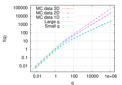
Figure 1: Scaling function $f_{d}(q)$ versus $q$.

Table 1: $B_{d}$ (5) for our trial points from MC simulations.

	1D	2D	3D
$q_{d}^{\min}$	0.5	1	1
$q_{d}^{\max}$	4 096	128	64
$B_{d}$	2.3285 (60)	2.0990 (53)	2.1427 (43)
$n_{d}$, $\chi^{2}_{d}({\rm pdf})$	6, 1.24	7, 1.07	10, 0.74

The results in 1D, 2D and 3D together with the analytical $q\to 0$ and $q\to\infty$ asymptotic behavior are presented in Fig. 1 on a log-log scale. When taking data our stepsize was a factor two in $q$. For crosschecks at a few $q$ values various combinations of $\tau^{0}_{\rm nu}$, $v$ and $V$ were used that combine to the same $q$ value.

Performing Gaussian difference tests (e.g., Ref. Bbook ), the first four data are in each case consistent with the small $q$ approximation (4). For $q\leq q_{d}^{\min}$, $q_{d}^{\min}$ listed in table 1, the data are found to agree with an relative error $|f_{d}(q)-f_{d}^{\rm small}(q)|/f_{d}(q)<5\%$ with the analytical small $q$ behavior. In the same way they are consistent with the large $q$ behavior (5) for $q\geq q_{d}^{\max}$, where the $B_{d}$ values listed in table 1 are determined by one-parameter fits to $n_{d}$ data with the largest $q$ values (chi-squared per degree of freedom of the fit, $\chi^{2}_{d}({\rm pdf})=\chi^{2}_{d}/(n_{d}-1)$, is also given). In the sense of these approximations we have nucleation for $q<q_{d}^{\min}$, spinodal decomposition for $q>q_{d}^{\max}$, and a crossover region in-between.

In particular, we have in this classification for a 3D cubic box $\tau_{\rm nu}/\tau_{\rm con}<0.02$ for spinodal decomposition and $\tau_{\rm nu}/\tau_{\rm con}>0.43$ for nucleation. While the coefficients $A_{d}$ and $B_{d}$ in Eqs. (4) and (5) depend on the geometry, the power laws do not. Therefore, they can be employed to characterize the limits universally.

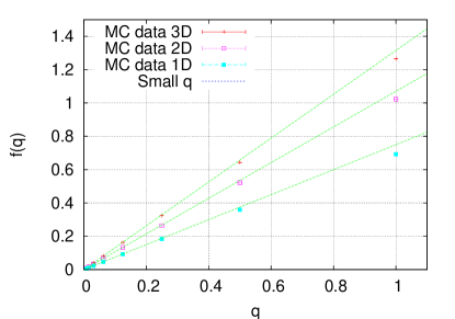
Figure 2: Scaling function: End of the small $q$ region (4).

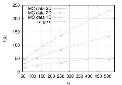
Figure 3: Scaling function: Beginning of the large $q$ region (5) in 2D and 3D.

In Fig. 2 we exhibit the end of the small $q$ region on a scale with higher resolution than that of the logarithmic scale of Fig. 1. Correspondingly the beginning of the large $q$ region in 2D and 3D is shown in Fig. 3. In 1D the asymptotic behavior sets in for considerably larger $q$ values. The reason appears to be that there are not yet sufficiently many nuclei participating in the phase conversion. At the largest $q$ value of Fig. 3 $(q=512)$ the deviation of the 1D MC result from its large $q$ asymptotics is still 11%.

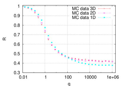
Figure 4: Ratio of contributing nuclei versus $q$.

The average number of participating nuclei, $N_{\rm nuclei}$ is smaller than $\tau_{\rm con}/\tau_{\rm nu}$ of Eq. (3) as nuclei created inside an already converted region do not contribute. In Fig. 4 we show the ratio $R=N_{\rm nuclei}/(\tau_{\rm con}/\tau_{\rm nu})$. For large $q$ it approaches $R=0.38$ in 1D and $R=0.42$ in 2D and 3D. These numbers are specific to our choice of trial points.

We continue with illustrations. Changes in physical conditions, for instance of the temperature, can influence the nucleation time $\tau^{0}_{\rm nu}$, the expansion speed $v$, and the volume $V$.

Let us assume a constant volume. If the nucleation time varies from $\tau_{\rm nu}\to\tau^{\prime}_{\rm nu}$ for fixed expansion velocity $v$, while we stay in the spinodal region $q>q_{d}^{\max}$, the scaling $q\to q^{\prime}=(\tau_{\rm nu}/\tau^{\prime}_{\rm nu})\,q$ yields for the conversion time change $\tau_{\rm con}^{\prime}=(\tau^{\prime}_{\rm nu}/\tau_{\rm nu})^{1/(d+1)}\,\tau_{\rm con}$. If in the same situation the nucleation time $\tau_{\rm nu}$ is fixed and the expansion speed varies from $v\to v^{\prime}$, we find for the new conversion time $\tau_{\rm con}^{\prime}=(v/v^{\prime})^{d/(d+1)}\,\tau_{\rm con}$. When staying in the nucleation region the corresponding equations are $\tau^{\prime}_{\rm con}=(\tau^{\prime}_{\rm nu}/\tau_{\rm nu})\,\tau_{\rm con}+A_{d}\,(\tau_{\rm nu}-\tau^{\prime}_{\rm nu})\,q$ and $\tau^{\prime}_{\rm con}/\tau_{\rm nu}=1+A_{d}\,(v/v^{\prime})\,q$, respectively.

Assume a 2D Ising model on a $100\times 100$ lattice is prepared in its initial state with all spins down. It is then simulated by Markov chain Monte Carlo Bbook below the critical temperature and with a magnetic field opposite to the initial orientation of the spins. For suitable choices of temperature and magnetic field the following numbers are realistic: (A) Seven nucleation events in one sweep with a subsequent expansion speed of 5 lattice spacings in 20 sweeps. (B) One nucleation event in 1680 sweeps and a subsequent expansion speed of 50 lattice site in 800 sweeps. A brief calculation puts case (A) with $q=2800$ solidly into the spinodal asymptotics, while with $q=0.95$ case (B) is at the end of nucleation region. Enlarging the lattice to $1\,000\times 1\,000$ sites moves case (B) to $q=953$ into the the spinodal region.

Consider a metastable liquid in a cubic box of size $(0.1\,{\rm meter})^{3}$ with a nucleation time of 1 minute in that volume and a subsequent explosion-like conversion at the speed of 100 km/h. With $q=6\times 10^{-5}$ this is deep in the nucleation region. This is no longer true if the same system is a pool of size $(10\,{\rm meter})^{3}$. Then we are at $q=6\,000$, though the preparation of such a large homogeneous system may in practice be impossible.

Conversion times of the order of minutes are observed in polyethylene crystallization Lu01 . To be definite, let $\tau_{\rm con}=180\,$s. If the nucleation time for the relevant volume is $\tau_{\rm nu}\leq 3.6\,$s, we would classify the process as spinodal decomposition, and for $\tau_{\rm nu}\geq 77.8\,$s as nucleation, with the crossover region in the range $3.6\,{\rm s}<\tau_{\rm nu}<77.8\,$s.

Let us consider the deconfining phase transition MO07 and choose $(1\,{\rm fermi})^{3}$ as the unit volume which defines $\tau^{0}_{\rm nu}$. Suppose the relevant volume at a heavy ion collider is of size $(10\,{\rm fermi})^{3}$, and that the deconfined phase spreads out at the speed of light once a nucleus is created. What is the range of nucleation times so that the phase conversion (confined $\to$ deconfined) proceeds by spinodal decomposition ($q\geq 64$)? The answer is $\tau^{0}_{\rm nu}<5\times 10^{-22}$ seconds. This estimate goes up when the expansion speed is slower than the speed of light.

Conclusions. Our equations will need corrections, once the critical nuclei can no longer be considered pointlike, and their size introduces a new dimensional parameter. Further, correlations between nuclei are presently neglected and the constant expansion speed of KJMA theory may be a too crude approximation for the actual dynamical, stochastic expansion process. Nevertheless, we think that the scaling laws outlined in this paper are at the heart of the distinction between nucleation and spinodal regimes of phase transitions.

- (1) G.S. Zhdanov, Crystal Physics, Oliver and Boyd, 1965.
- (2) R.E. Smallman and A.H.W. Ngan, Physical Metallurgy and Advanced Materials, 7th edition, Butterworth-Heinemann, 2007.
- (3) K. Binder (editor), Monte Carlo and Molecular Dynamics Simulations in Polymer Science, Oxford University Press, USA, 1995.
- (4) G. Stroble, The Physics of Polymers: Concepts for Understanding Their Structures and Behavior, 3rd edition, Springer, 2007.
- (5) Y. Ishibashi and Y. Takagi, J. Phys. Soc. Japan 31, 506 (1971); M. Okuyama and Y. Ishibashi (editors), Ferroelectric Thin Films: Basic Properties and Device Physics for Memory Applications (Topics in Applied Physics), Springer, 2005.
- (6) P.A. Rikvold and B.M. Gorman in Annual Reviews of Computational Physics I, D. Stauffer (editor), World Scientific 1994.
- (7) D.P. Landau and K. Binder, A Guide to Monte Carlo Simulations in Statistical Physics, Cambridge University Press, 2000.
- (8) H. Meyer-Ortmanns and T. Reisz, Principles of phase structures in particle physics, World Scientific 2007.
- (9) L. O’Malley, B. Kozma, G. Korniss, Z. Rácz, and T. Caraco, Phys. Rev. E 74, 041116 (2006) and references therein.
- (10) Here we use the terminology “spinodal decomposition” and “spinodal conversion” in a broader sense than some statistical physicists do.
- (11) J.S. Langer, in Solids far from Equilibrium, C. Godreche (editor), Cambridge University Press, 1992.
- (12) A.N. Kolmogorov, Bull. Acad. Sci. USSR, Ser. Math. 3, 355 (1937).
- (13) W.A. Johnson and P.A. Mehl, Trans. Am. Inst. Min. Metall. Eng. 135, 416 (1939).
- (14) M. Avrami, J. Chem. Phys. 7, 1103 (1939); 8, 212 (1940); 9, 177 (1941).
- (15) The nuclei are also called droplets, for instance in Ref. RG94 .
- (16) U.R. Evans, Trans. Faraday Soc. 41, 365 (1945).
- (17) K. Sekimoto, Int. J. Mod. Phys. B 5, 1843 (1990).
- (18) A.A. Burbelko, E. Fraś, and W. Kapturkiewics, Mat. Sci. and Eng. A 413, 429 (2005).
- (19) B.A. Berg (unpublished).
- (20) P.A. Rikvold, H. Tomita, S. Miyashita, and S.W. Sides, Phys. Rev. E 49, 5080 (1994); M.A. Novotny, G. Brown, and P.A. Rikvold, J. Appl. Phys. 91, 6908 (2002).
- (21) B.A. Berg, Markov Chain Monte Carlo Simulations and Their Statistical Analysis, World Scientific, 2004.
- (22) X.F. Lu and J.N. Hay, Polymer 42, 9423 (2001); J. Suh and J.L. White, J. Appl. Polymer Sci. 106, 276 (2007).