Large Magnetoresistance in a Manganite Spin-Tunnel-Junction
Using LaMnO₃ as Insulating Barrier

Abstract

A spin-tunnel-junction based on manganites, with La_1-xSr_xMnO₃ (LSMO) as ferromagnetic metallic electrodes and the undoped parent compound LaMnO₃ (LMO) as insulating barrier, is here theoretically discussed using double exchange model Hamiltonians and numerical techniques. For an even number of LMO layers, the ground state is shown to have anti-parallel LSMO magnetic moments. This highly resistive, but fragile, state is easily destabilized by small magnetic fields, which orient the LSMO moments in the direction of the field. The magnetoresistance associated with this transition is very large, according to Monte Carlo and Density Matrix Renormalization Group studies. The influence of temperature, the case of an odd number of LMO layers, and the differences between LMO and SrTiO₃ as barriers are also addressed. General trends are discussed.

I Introduction

The study of strongly correlated electronic systems (SCES) continues attracting the attention of the Condensed Matter community. These materials present complex phase diagrams that illustrates the competition which exists among phases with very different physical properties, such as $d$-wave superconductivity, antiferro- and ferro-magnetic order, charge- and orbital-order, multiferroic behavior, and several others. Moreover, this complexity and phase competition lead to self-organized nano-scale inhomogeneities which are believed to generate giant responses, as in the famous colossal magnetoresistance (CMR) effect of the Mn-oxides known as manganites.dagotto-CMR

Recently, a new procedure to study oxide SCES has been proposed. It involves the artificial creation of oxide multilayers with atomic-scale accuracy at the interface, via the use of techniques such as pulsed-laser deposition.multilayers Potentially, these structures can have properties very different from those of the building blocks. One of the reasons for this expectation is that a transfer of charge could occur between the constituents leading, for example, to the stabilization of a metal at the interface between two insulators.multilayers The creation of novel two-dimensional states, as well as the possible applications of oxide multilayers in the growing field of oxide electronics, has given considerable momentum to these investigations.

I.1 Spin-Tunnel-Junctions

The development of the above mentioned accurate experimental techniques for the construction of oxide multilayers with atomic precision can have implications in the study of spin-tunnel-junctions,junctions ; junctions-reviews introducing a better control of their properties. These structures consist of two ferromagnetic (FM) metallic electrodes, separated by a thin insulating barrier. The resistance of this device depends on the relative orientation of the electrodes’ magnetizations. The tunneling magnetoresistance (TMR) is usually defined via the difference in resistances between the anti-parallel and parallel arrangements of the electrodes’ magnetic moments. Half-metals, such as La_1-xSr_xMnO₃ (LSMO), with an intrinsic nearly full magnetization, are ideal for these devices.half-metal

In the context of magnetic tunnel junctions, very interesting results were reported by Bowen et al. bowen using a LSMO/STO/LSMO trilayer. The Sr concentration was 1/3 for La_1-xSr_xMnO₃ (LSMO), and STO represents the insulator SrTiO₃. A huge TMR ratio of more than 1800% was observed at very low temperatures 4 K, showing the advantages of using half-metallic LSMO as a ferromagnetic electrode in the junctions. However, in the same investigations it was reported that the large TMR survived only up to $\sim$270 K, lower than the Curie temperature of LSMO($x$=1/3), which is $\sim$370 K. It was argued that the deterioration of the ferromagnetism near the LSMO/STO interface (“dead layer”) could be causing this TMR reduction. Later, Yamada et al. yamada addressed this problem by comparing the STO/LSMO interface with others, such as LAO/LSMO or STO/LMO/LSMO, where LAO stands for LaAlO₃ and LMO for LaMnO₃. Those authors found that the magnetic behavior of LAO/LSMO and STO/LMO/LSMO are much better than STO/LSMO in the sense that no dead-layer was found, opening a new path toward LSMO-based TMR junctions operating at room temperature.

I.2 Proposed Main Idea

In this paper, an alternative setup is proposed for a manganite trilayer system which is expected to have a very large magnetoresistance (MR) at low temperatures, at least according to modeling calculations reported below. The proposed geometry, and main idea behind its performance, is presented in Fig. 1. The new system is made out entirely of manganite materials, with different hole doping concentrations.jo Using all manganites may help in the interfacial contact between the components due to their similar lattice spacings. More specifically, in Fig. 1 (a) a trilayer system is represented. It contains two hole-doped Mn-oxides, such as LSMO, and a central region made out of the undoped parent compound LMO. It is well known that LSMO is ferromagnetic and half-metallic for sufficiently large hole doping, while LMO is an A-type antiferromagnetic (AF) insulator. dagotto-CMR The arrows in Fig. 1 (a) represent schematically the expected spin orientations in a one-dimensional arrangement, for simplicity. The most interesting detail of Fig. 1 (a) is the relative orientation of the spins between the metallic leads. For an $even$ number of layers in the central LMO region, the ferromagnetic moments of the leads are $anti$-$parallel$. This is expected to cause a very large resistance at low temperatures, since the carriers moving from one lead to the other not only must tunnel through the central insulating barrier, but in addition the spin species which can travel in one lead is blocked by the other. However, the anti-parallel configuration, which is mediated by the central region, is not strongly pinned in this arrangement: it is only a $weak$ antiferromagnetic effective interaction which produces the ground state with anti-parallel leads’ moments. Thus, relatively small magnetic fields can render the ferromagnetic moments parallel, substantially reducing the resistance. All these intuitive ideas will be substantiated via model calculations, described below.

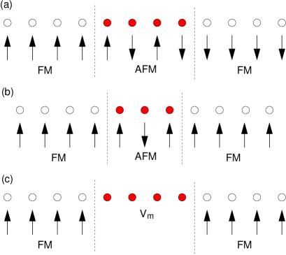
Figure 1: (Color online) Schematic representation of a one-dimensional (1D) double exchange (DE) model for a LSMO/LMO/LSMO trilayer with even (a) and odd (b) numbers of LMO sites. Here, LMO and LSMO represent regions where the positive background charge densities correspond to an antiferromagnetic (AFM) insulator and ferromagnetic (FM) metal, respectively, when in bulk form. Circles stand for lattice sites where electrons can move, and arrows indicate localized spins. The trilayer with even (odd) number of LMO sites gives rise to anti-parallel (parallel) alignment of the magnetic moments in the left and right ends of LSMO. (c) Schematic representation of a 1D model for a LSMO/STO/LSMO trilayer. Here, LSMO is described by the DE model as before, while STO is modeled by a tight-banding model with no localized spins. $V_{\rm m}$ introduced in the central STO region is a band off-set site-potential mimicking the work function difference between LSMO and STO. More details can be found in the text.

For an $odd$ number of layers in the central LMO region, the expected spin arrangement is shown in Fig. 1 (b). In this case the magnetic moments of the leads will be parallel to one another, and the resistance will not be as large as for the configuration shown in Fig. 1 (a). However, the LMO region still provided a tunneling barrier, and the performance of this case will be shown below to be quite acceptable, at least within modeling calculations.

Finally, Fig. 1(c) contains a crude representation of a more standard trilayer device. bowen While the leads are still representing LSMO, the central region is now a band insulator, as it occurs in the much employed case of STO. The main focus of our effort will be the cases shown in Fig. 1 (a) and (b), but some results for the setup shown in Fig. 1 (c) will also be discussed for completeness, and to clarify qualitative trends.

I.3 Main approximations

Before proceeding to the presentation of the results, some of the theoretical approximations used must be clearly expressed for the benefit of the reader. With this paper, our main intention is to motivate experimental groups to consider the materials and setups proposed in our study, involving a magnetically active manganite barrier, as opposed to a magnetically-inert band-insulator, as the widely used STO. However, it must be clearly stated that our calculations are qualitative at best and should be considered only as a guidance to understand the intuitive picture presented here.

A variety of effects are not taken into account in this investigation (and actually these effects cannot be taken into account accurately within the current status of numerical simulations and Hamiltonian modeling). (1) For instance, the lattice and orbital reconstructions are not incorporated, but only the electronic reconstruction is considered. In other words, the atomic positions are considered to be rigid here. It would be the task of sophisticated ab-initio simulations to consider how the lattice relaxes at the interface between LMO and LSMO, and such future calculations are certainly strongly encouraged. (2) A second subject which is not addressed in this work is the issue of the infamous “dead layer” at the barrier/electrode interface, already briefly described in Sec. I.1. Dead layers affect the performance of several trilayer devices. We have attempted to mimic this dead layer altering by hand the chemical potential in the vicinity of the interface, but the results were not sufficiently satisfactory to be described in this paper. Thus, this problem is left for future efforts. (3) Another topic which is only briefly discussed is the influence of anisotropies: in most of the simulations below there is no “easy” axis introduced for the magnetization orientation. While for manganites in bulk form this is a reasonable assumption, in thin films it is known that in-plane magnetic anisotropies are induced by epitaxial strain.mathews These anisotropies are the reason behind the abrupt changes in resistances observed when varying magnetic fields in magnetic tunnel junctions (see, for instance, Fig. 2 in Ref. bowen, ). While in our numerical studies reported below the simulations are carried out mainly with isotropic Heisenberg spins, a more proper analysis would have needed anisotropic terms, rendering these spins Ising like. (4) A related topic involves the experimentally observed differences between the upper and lower electrodes in a trilayer junction, since the area of the bottom electrode is typically much wider than that of the upper one.ishii This stabilizes anti-parallel orientations of the electrodes’ magnetic moments at some magnetic fields. In our simulations, both electrodes are perfectly equivalent. However, for the reasons already mentioned in the previous subsection, we do stabilize a similar anti-parallel magnetic moment arrangement via the use of LMO as barrier, with an even number of sites and in zero external magnetic field. (5) Finally, a practical assumption in our investigations is the focus on a one-dimensional (1D) spin arrangement, described by the realistic double-exchange model for manganites (albeit restricted to just one orbital). The restriction to a 1D configuration is needed for the numerical studies to be accurate; higher dimensional arrangements would have increased so much the CPU time that a careful analysis would have been impossible. Note that contrary to manganite bulk studies,dagotto-CMR where the analysis of small two-dimensional clusters is possible, here we will be carrying out an iterative loop to solve Poisson’s equation which regulates the charge transfer between materials (see Sec.II). At each step of the iterative process, an entire Monte Carlo (MC) process or Density Matrix Renormalization Group (DMRG) sweep is carried out (see details below), thus increasing substantially the computer requirements. Then, the restriction to a 1D geometry is caused by the CPU resources available. However, in the description of results below, we have focus on qualitative aspects which are expected to be robust, and we strongly believe that they will survive the increase in dimensionality. For example, the large magnetoresistance at low temperatures of the LSMO/LMO/LSMO setup, with an even number of layers for LMO, is believed to occur in any dimension of interest.

I.4 Organization

The organization of the paper is the following. In Sec. II, the model Hamiltonians and numerical methods are described. The focus is on Monte Carlo and DMRG techniques. The main results are presented in Sec. III, which correspond to the arrangements schematically described in Fig. 1 (a) and (b), showing that the magnetoresistance is large in these setups. Both classical and quantum localized $t_{\rm 2g}$ spins are used. In Sec. IV, the influence of temperature is analyzed. As observed in some experiments, bowen it is found that the large MR effect quickly deteriorates with increasing temperature. The influence of anisotropies is also studied as a possible cure to this problem. In Sec. V, for completeness, results of the modeling of a trilayer involving a band insulator (such as STO) as the barrier, instead of LMO, are reported. Conclusions are given in Sec. VI.

II Model and methods

II.1 Model Hamiltonian and MC methods

To crudely model LSMO/LMO/LSMO trilayers (Fig. 1), the one-orbital double exchange (DE) model on a 1D lattice will be used:

$$H = -t\sum_{\langle i,j\rangle}\sum_{\sigma}\left(c_{i,\sigma}^{\dagger}c_{j,\sigma}+{\rm H.c.}\right)+\sum_{i}\phi(i)n_{i}$$ (1)

$$-J_{\rm H}\sum_{i}{\cal{\bf s}}_{i}\cdot{\bf S}_{i}-\sum_{i}{\bf h}_{\rm ext}\cdot{\bf M}_{i},$$

where $c_{i,\sigma}^{\dagger}$ is the creation operator of an electron at site $i$ with spin $\sigma(=\uparrow,\downarrow)$. The first summation of $\langle i,j\rangle$ runs over nearest neighbor pairs of sites $i$ and $j$. The number operator is $n_{i}=\sum_{\sigma}c_{i,\sigma}^{\dagger}c_{i,\sigma}$, $\phi(i)$ is the electrostatic potential (discussed below), and the spin operator of the electron is ${\bf s}_{i}=\sum_{\alpha,\beta}c_{i,\alpha}^{\dagger}\left({\vec{\sigma}}\right)_{\alpha\beta}c_{i,\beta}$ (here ${\vec{\sigma}}=(\sigma_{x},\sigma_{y},\sigma_{z})$: Pauli matrices). ${\bf S}_{i}$ is the classical spin, widely used to represent the localized $t_{\rm 2g}$ spins, with $|{\bf S}_{i}|$=$1$. $J_{\rm H}$ is the Hund’s rule coupling, ${\bf h}_{\rm ext}$ is an external magnetic field, and ${\bf M}_{i}$=${\frac{1}{2}}({\bf s}_{i}+3{\bf S}_{i})$ is the total magnetic moment at site $i$. Hereafter, $t$ is set to be 1 as an energy unit. The number of sites in the left, central, and right regions of the system is denoted by $L^{(\rm L)}$, $L^{(\rm C)}$, $L^{(\rm R)}$, respectively.

To study the electronic properties of hetero-structured systems, it is crucial to include the cation ions in the model (to consider the charge neutrality condition) and take into account long-range Coulomb interactions between electrons and cation ions. In this study, the long-range Coulomb interactions are considered within the Hartree approximation through Poisson’s equation: datta

$$\nabla^{2}\phi(i)=-\alpha\left[\langle n_{i}\rangle-n_{+}(i)\right],$$ (2)

where $n_{+}(i)$ is the positive background charge mimicking the cation ions. Here in this paper, $n_{+}(i)$=$n^{(\Gamma)}$ is set to be uniform within each layer [$\Gamma$=${\rm L}$ (left region), C (central region), and R (right region)], with a value determined by the charge neutrality condition. The parameter $\alpha$=$e^{2}/\varepsilon a$ ($e$: electronic charge, $\varepsilon$: dielectric constant, $a$: lattice constant) is the strength of the Coulomb interactions, considered as a free parameter in the model. To solve Eq. (2), the symmetric discretization of Poisson’s equation is used, which in 1D becomes $\nabla^{2}\phi(i)$=$\phi(i+1)-2\phi(i)+\phi(i-1)$, with boundary conditions $\phi(i)$=$0$ for sites outside of the system.

In the following sections, results for zero temperature ($T$) as well as finite temperatures are reported. For the finite temperature calculations, the standard grand-canonical Monte Carlo simulation is used, yunoki with the chemical potential $\mu$ adjusted such that the total number of electrons are equal to the total background positive charge $\sum_{i}n_{+}(i)$. For the zero temperature calculations, a full optimization of $\{{\bf S}_{i}\}$ using the Broyden-Fletcher-Goldfarb-Shanno method NR is performed for a fixed number $N$ of electrons, i.e., $N=\sum_{i}n_{+}(i)$ (canonical ensemble). We have found that the Monte Carlo simulations at very low temperatures produce almost identical results as those calculated using the zero temperature canonical method, although at a considerably larger cost in CPU time. Thus, at $T$=0 it is advantageous to use the optimization method. Note that due to the need to solve Poisson’s equation iteratively, a Monte Carlo simulation or optimization procedure has to be carried out at each step, increasing substantially the computer time as compared with more standard simulations of bulk systems. The calculation of the conductances is carried out using the Landauer formalism, verges as extensively explained in previous reports. dagotto-CMR ; dagotto-book

In the real LSMO/STO/LSMO trilayer systems, which will also be briefly modeled in this manuscript, it is important to notice that there exists band offsets (due to work-function differences) between LSMO and STO, which are typically of the order of a few eVs, sawa although its precise value is difficult to find experimentally.electron-doped In this paper, this band offset is treated as a parameter described simply by the addition of a site potential term $V_{m}\sum_{i\subset{\rm C}}n_{i}$ to the Hamiltonian [Fig. 1 (c)]. Moreover, a simple tight-binding model without $J_{\rm H}$ in Eq. (1) is used to model the STO barrier. Omitting Hubbard-type interactions might be justified by the fact that the number of electrons in the central region (STO) is very small, as shown later. And for LSMO and LMO, neglecting the Hubbard term is justified by the large value of the Hund’s coupling which by itself prevents double occupancy, as widely discussed before.dagotto-CMR

II.2 Quantum localized spins and DMRG

Results using quantum spin 1/2 for the localized spins ${\bf S}_{i}$ in Eq. (1) are also presented in this paper, and they are compared with results of the classical spin simulations. In real manganites $t_{\rm 2g}$ spins are 3/2. However, using spin 1/2 much simplifies the computational task due to the reduction in the size of the Hilbert space. yunoki To study the ground state properties of Eq. (1) with ${\bf S}_{i}=1/2$, e.g., the charge density distribution, the standard DMRG algorithm,DMRG embedded in a self-consistent iterative procedure to solve Poisson’s equation for the long-range Coulomb potential, is used.

More specifically, starting from an initial electrostatic potentials $\phi(i)$ ($i=1,\ldots,L$, here $L$ is number of total sites), we first make two sweeps for “warming” before beginning the self-consistent calculations for the long-range Coulomb interactions. Then, for the next 10 sweeps, the electrostatic potentials $\phi(i)$ are updated by solving Poisson’s equation [Eq. (2)] at each sweep. In general, the convergence of the self-consistent procedure is very slow. Therefore, here we perform an extrapolation of $\phi(i)$ for each $i$, using the values calculated during those 10 sweeps, to an infinite number of sweeps. By comparing fully self-consistent calculations, we have found that generally this extrapolation scheme gives a reasonable results. Finally, the obtained potential $\phi(i)$ is plugged back in Eq. (1), and 8 more sweeps are performed to calculate the ground state. The results reported below are obtained by retaining $M$=$350$ states, and the truncation error in the worst case is of order $10^{-7}$. All DMRG calculations are done at $T=0$, and $J_{\rm H}$=36 is used. yunoki

As a check of our DE model code, we have compared the case of a total $z$-projection of the spin $S_{z}=S_{\rm max}$=$26$, on a lattice of $L$=$32$ sites and with a total number of conduction electrons $N=20$, with the results of the spinless fermion model which is computed with a previously prepared DMRG code for the Hubbard model, seba written completely independently from the present DE code. The potential $\phi(i)$ added in the spinless fermion calculation is the one extracted from the DE run. The differences in energies are found to be of order $10^{-7}$.

To study transport properties, the time-dependent DMRG technique is used.tDMRG The electrostatic potentials $\phi(i)$ are fixed to the ones obtained above, and a small bias potential $\Delta V$=$0.01$ is applied at time $t$=$0$, which triggers a time-evolution of the system. alhassanieh The bias potential is applied only on a few sites at the edges of the system, and the current as a function of $t$ is measured on the two links connecting the central region to the two outer portions of the system. The amplitude of $J(t)$, defined as the average of these two currents, scales approximately linearly with the number of sites on which the bias potential $\Delta V$ is applied. As it is well known,alhassanieh $J(t)$ follows an oscillatory evolution with time due to the open boundary conditions used in the DMRG process (electrons cannot leave the system). Thus, to obtain a measure of the conductance, the average of $J(t)/\Delta V$ over the first half-period of the oscillation is considered.alhassanieh

III Results at zero temperature

In this section, the main results obtained in our numerical simulations will be described.

III.1 All-manganite trilayer geometry
using classical $t_{\rm 2g}$ spins

III.1.1 Even number of sites in the barrier

Figure 2 shows the zero-temperature optimization results corresponding to a 1D trilayer geometry [Fig. 1 (a)] consisting of 20 sites in each lead, and 4 sites in the middle. The positive charge, regulated by $n_{+}$, is 0.65 at each lead and 1.0 in the middle (in $e$=1 units). The strength of the long-range Coulomb interaction is chosen as $\alpha$=1.0. Figure 2(a) shows the converged local electronic density $n(i)$ vs. the site location $i$, along the 44 sites chain. In the leads, the electronic density closely matches the expected result 0.65. The oscillations at the end of the chain near $i$=1 and 44 are due to Friedel oscillations. In the 4-sites center, 2 of the sites have $n(i)$ very close to 1, while the other 2 have a smaller density due to the charge-transfer effect of the long-range forces. The overall electronic density profile is reasonable and in agreement with qualitative expectations.

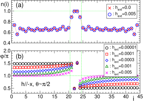
Figure 2: (Color online) (a) Local electron density $n(i)$ and (b) classical spin orientation ${\bf S}_{i}=(\theta_{i},\varphi_{i})$ ($0\leq\theta_{i}\leq\pi$, $0\leq\varphi_{i}\leq 2\pi$) in spherical coordinates vs. site location $i$, on a trilayer chain with $L^{(\rm L)}=L^{(\rm R)}=20$ sites in each lead and $L^{(\rm C)}=4$ sites in the center. The 1D DE model with $J_{\rm H}$=$8.0$ and $\alpha$=$1.0$ is used, and the results are obtained via an optimization method at zero temperature. Lead’s positive background charge is $n_{+}^{(\rm L)}$=$n_{+}^{(\rm R)}$=$0.65$, and a central positive background charge is $n_{+}^{(\rm C)}$=$1.0$. A magnetic field is applied in the direction opposite to $x$-direction (x), and the magnitude ($h_{\rm ext}$) is shown in the figures. In (b), $\theta_{i}\sim\pi/2$ for all $h_{\rm ext}$’s. As $h_{\rm ext}$ increases, the spins gradually rotate toward $-{\bf x}$ in the $xy$ plane, and finally they align ferromagnetically. The positions of the two interfaces are denoted by vertical dashed lines.

The lower panel Fig. 2(b) contains the most important result for this particular geometry. There, the orientations of the classical $t_{2g}$ spins are shown via the spherical coordinates angle $\varphi$, as a function of position $i$. Note first that each lead has classical $t_{\rm 2g}$ spins polarized in a ferromagnetic state, namely all sites have approximately the same $\varphi$, as expected from the well-known double-exchange mechanism. zener This ferromagnetism at the leads is compatible with phase diagrams gathered in previous studies.yunoki However, in the near absence of magnetic fields, $h_{\rm ext}$=0.00001, the angle $\varphi$ of the two ferromagnetic leads differs by $\pi$, signaling an anti-parallel arrangement of magnetic moments between the two ferromagnetic leads (the tiny field was used simply to orient the spins along a direction which simplifies the discussion, and it does not have any other important effect). This anti-parallelism is in excellent agreement with the expected results based on the introductory discussion: if the number of sites in the antiferromagnetic barrier is even, then an anti-parallel orientation of ferromagnetic moment between the leads should occur. In the barrier region, the classical spins are arranged in an antiferromagnetic pattern, since there $n(i)$$\sim$1 and an antiferromagnetic spin orientation is preferred. yunoki

The results become even more interesting as the magnetic field is increased. In this case, the relative orientation of the ferromagnetic moments in the leads changes very rapidly, as shown in Fig. 2(b). For fields as small as $h_{\rm ext}$=0.005 (in units of the hopping $t$), the magnetic moments of the ferromagnetic leads are already nearly aligned. As shown below, this produces drastic changes in the conductance of the ensemble. Results for intermediate values of the magnetic field, also in Fig. 2(b), show that the transition from anti-parallel to parallel orientation of the ferromagnetic lead’s moments is smooth and, moreover, noticeable changes can be observed even for fields as tiny as $h_{\rm ext}$=0.0001 (a discussion of how small this field is in physical units is below).

The relative orientation of the magnetic moments of the leads, and their rotation with magnetic fields, induce substantial modifications in the conductance and a concomitant large magnetoresistance. Figure 3(a) shows the conductance of the trilayer vs. magnetic field $h_{\rm ext}$. At fields zero or very small, the anti-parallel orientation of the lead’s moments produces a very small conductance. This is reasonable since the spin orientation which can conduct in one lead, is blocked by the anti-parallel lead. However, as $h_{\rm ext}$ increases, there are substantial changes in the conductance. For fields as small as $h_{\rm ext}$=0.0002, the conductance has changed by about 3 orders of magnitude already, at least for the particular system studied here. Note that if $t$ is assumed to be 0.1 eV, then $h_{\rm ext}$=0.0001 is approximately 0.1 T. The conductance increases further, by more than an order of magnitude, by increasing $h_{\rm ext}$ toward the value 0.003 where the moments of the leads become essentially parallel. The conductances remain in absolute value much smaller than the perfect conductance $2e^{2}/h$ ($h$: Planck constant), but its relative changes can be large, as illustrated in Fig. 3(b). In the widely used definition for conductance changes, which has the zero field conductance in the denominator, the magnetoresistance ratio can be very large, and it reaches almost 200,000% at $h_{\rm ext}$=0.001.

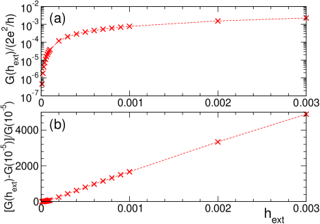
Figure 3: (Color online) (a) Conductance $G(h_{\rm ext})$ in units of $2e^{2}/h$ ($h$: Planck constant) and (b) magnetoresistance (MR) ratio, as a function of an applied magnetic field $h_{\rm ext}$. The results are calculated for the 1D DE model with $J_{\rm H}$=$8.0$, $\alpha$=$1.0$, and $T$=$0.0$. Positive background charges are $n_{+}^{(\rm L)}$=$n_{+}^{(\rm R)}$=$0.65$ and $n_{+}^{(\rm C)}$=$1.0$, and leads and central region sizes are $L^{(\rm L)}$=$L^{(\rm R)}$=$20$ and $L^{(\rm C)}$=$4$, respectively. To estimate the MR ratio, defined in the vertical axis of (b), $G(h_{\rm ext})$ with $h_{\rm ext}=10^{-5}$, instead of $G(h_{\rm ext}=0)$, is used since the conductance at $h_{\rm ext}$=0 vanishes. Note that with increasing $h_{\rm ext}$ the conductance $G(h_{\rm ext})$, and the MR ratio, increases almost linearly except for very small $h_{\rm ext}$ ($\lesssim 0.0003$).

To give a better perspective of the importance of these numbers, note that in a recent numerical studysen of the same model used for the trilayer geometry but defined on a finite two-dimensional cluster without interfaces, the CMR phenomenon was observed for larger magnetic fields $h_{\rm ext}$=0.05. In this case the MR magnitude was 10,000% at the best. Thus, the trilayer geometry investigated here certainly produces a more dramatic effect at smaller fields than in the bulk simulations.

To help experimental readers who are more used to resistance plots, in Fig. 4(a), the resistance $R$ of the trilayer with an even number of sites in the barrier is shown as a function of magnetic field $h_{\rm ext}$. Notice the rapid change in $R$ at small $h_{\rm ext}$, which is the main result of this paper. In experimental similar plots, such as those reported for STO and LAO as barriers, hysteresis loops are often observed in TMR vs. $h_{\rm ext}$, and moreover the effects at tiny fields are negligible. bowen ; yamada ; ishii These differences are caused by the anisotropies present in real experiments due to strain in the samples, as briefly explained in Sec. I.3, effect that has been mainly neglected in our calculations (with the exception of the results shown in Fig. 15 below). In Fig. 4(b), magnetization $M$ of the classical $t_{2g}$ spins for the trilayer ensemble vs. $h_{\rm ext}$ is shown. Compatible with the spin arrangements already described, there is no net magnetization $M$ at $h_{\rm ext}$=0, since the contributions of the ferromagnetic leads cancel out. However, with increasing $h_{\rm ext}$, there is a rapid increase in $M$ because the lead’s magnetic moments are aligning in the same direction. The subsequent small increases in $M$ and decrease in $R$, say for $h_{\rm ext}$=0.001 or larger, are due to further fine alignment of the spins close to the central region (the spin orientation in the central region remains antiferromagnetic, which eventually turns to FM with much larger $h_{\rm ext}$). Thus, the effective height of the barrier melts as $h_{\rm ext}$ (or $T$, as discussed in the next section) increases in this system.

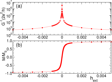
Figure 4: (Color online) (a) Resistance (inverse of conductance) vs. magnetic field $h_{\rm ext}$ for an even number of sites $L^{(\rm C)}$=4 in the central barrier at zero temperature. The leads each has $L^{(\rm L)}$=$L^{(\rm R)}$=20 sites, and the positive background charges are $n_{+}^{(\rm L)}$=$n_{+}^{(\rm R)}$=$0.65$ and $n_{+}^{(\rm C)}$=$1.0$ in the leads and central region, respectively. The couplings used are $J_{\rm H}$=$8.0$, and $\alpha$=$1.0$. Notice that the large changes in resistance occur at very small magnetic fields. (b) Total magnetization $M$ of the classical $t_{2g}$ spins vs. $h_{\rm ext}$, indicating the rapid development with $h_{\rm ext}$ of a net magnetization. $M_{S}$ is the maximum possible magnetization.

III.1.2 Odd number of sites in the barrier

The numerical results obtained for the case of an odd number of sites in the barrier are very different from those reported thus far. In Fig. 5, the results for the case of $L^{(\rm C)}=5$ sites in the barrier are reported. Fig. 5 (a) shows the electronic density $n(i)$ vs. $i$, which is similar to the results for the case of $L^{(\rm C)}=4$ sites in the barrier [Fig. 2 (a)]. The electrostatic potential for electrons $\phi(i)$, caused by the long-range Coulomb interactions, shown in Fig. 5 (b), is also canonical: in the central region more electrons are expected to accumulate since there $n_{+}(i)$ is larger than in the leads. The important qualitative difference with the previous results in Sec. III.1.1 is presented in Fig. 5 (c). Here, the spin correlation functions for the classical $t_{2g}$ spins indicate that the magnetic moments of the leads are parallel to each other, even in the absence of magnetic fields. This is in agreement with the qualitative scenario for these geometries described in the introduction (Sec. I.2). As a consequence, the case of an odd number of sites in the barrier does $not$ present the same huge magnetoresistance at small magnetic fields as for the even case.

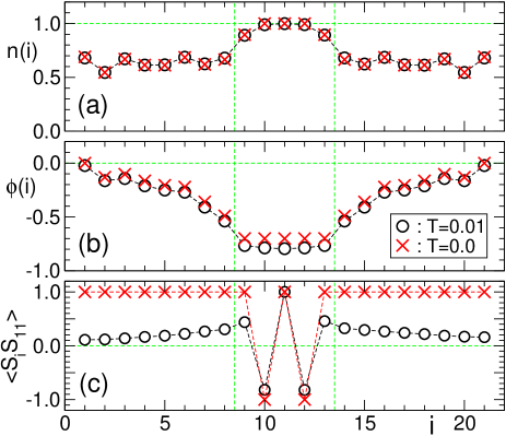
Figure 5: (Color online) (a) Local electron density $n(i)$, (b) electrostatic potential $\phi(i)$, and (c) classical $t_{2g}$ spin correlation function $\langle{\bf S}_{i}\cdot{\bf S}_{j}\rangle$ from the central site at $j$=$11$. The Monte Carlo techniques and optimization method are used for the 1D DE model with $J_{\rm H}$=$8.0$ and $\alpha$=$2.0$ at $T$=$0.01$ and $T=0$, respectively. The positive background charges are $n_{+}^{(\rm L)}$=$n_{+}^{(\rm R)}$=$0.625$ and $n_{+}^{(\rm C)}$=$1.0$, and the system size used is $L^{(\rm L)}$=$L^{(\rm R)}$=$8$ and $L^{(\rm C)}$=$5$. Here, $\phi(i)$ is self-consistently determined. The interface positions are denoted by vertical dashed lines.

The resistance $R$ vs. magnetic field $h_{\rm ext}$ is shown in Fig. 6(a). As in the case of the even $L^{(\rm C)}$, clearly $R$ decreases with increasing $h_{\rm ext}$. However, the scales involved are very different. While for $L^{(\rm C)}$ even, there are huge changes at $h_{\rm ext}$ as small as 0.0001 (Fig. 4), for the $L^{(\rm C)}$ odd case the resistance remains almost the same up to $h_{\rm ext}$=0.02. The reason is that the magnetic field does not need to align the magnetic moments of the leads in this case (they are already aligned), and moreover the up-down-up arrangement of the central region is compatible with the parallel leads’ moments. The only modification needed in the spin arrangement is the correction in the orientation of the central spins that are pointing the wrong way. This process takes place between fields $h_{\rm ext}$=0.02 and 0.05 approximately. After that, the entire system is ferromagnetic and the resistance remains constant. For completeness, Fig. 6(b) shows the total magnetization of the classical $t_{2g}$ spins. As expected, initially, $M$ is very robust, and it becomes saturated at $h_{\rm ext}\sim 0.05$.

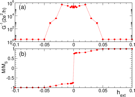
Figure 6: (Color online) (a) Resistance (inverse of conductance) vs. magnetic field $h_{\rm ext}$ for an odd number of sites $L^{(\rm C)}$=5 in the central barrier at $T$=1/800. The leads have $L^{(\rm L)}$=$L^{(\rm R)}=8$ sites, and the positive background charges are $n_{+}^{(\rm L)}$=$n_{+}^{(\rm R)}$=$0.625$ and $n_{+}^{(\rm C)}$=$1.0$ for the leads and central region, respectively. The couplings used are $J_{\rm H}$=$8.0$ and $\alpha$=$1.0$. (b) Total magnetization $M$ of the classical $t_{2g}$ spins vs. magnetic field $h_{\rm ext}$, indicating that the system is overall ferromagnetic at all magnetic fields. $M_{S}$ is the maximum possible magnetization. $\phi(i)$ is determined self-consistently at $T$=$0.2$ and $h_{\rm ext}=0$, and then used for other temperatures and $h_{\rm ext}$ (see more details in the text).

III.2 All-manganite trilayer geometry
using quantum $t_{\rm 2g}$ spins

The existence of parallel or anti-parallel arrangements of the magnetic moments in the left and right leads is also investigated for the 1D DE model with quantum localized $t_{2g}$ spins ${\bf S}_{i}$ [Eq. (1)] at $T=0$ by the DMRG technique. For numerical simplicity, spin-1/2 is employed, instead of the realistic value 3/2.

In Fig. 7, the ($z$-component) spin correlation functions $\langle S^{z}_{i}S^{z}_{j}\rangle$ are reported for a typical set of parameters, choosing one of the central-region spins ($j=0$) as a reference. There are 4 and 5 sites in the central region in Fig. 7 (a) and (b), respectively. In the case of even number of central sites [Fig. 7 (a)], at least for large values of $\alpha$ such as 2, the antiferromagnetic spin correlations in the central region are clearly observed, and moreover the magnetic moments of the left and right leads tend to align anti-parallel. However, quantum fluctuations, enhanced by the spin-1/2 and one-dimensionality nature of the model, make the spin correlations at longer distances weaker, and the correlations become very small for $|i|\gtrsim 4$. Similarly, quantum fluctuations reduce spin correlations at large distances also for odd number of central sites, shown in Fig. 7 (b). However, in this case, a tendency of parallel alignment of the magnetic moments between the left and right leads can still be observed. Thus, overall features observed in the case of quantum $t_{2g}$ spins are in good qualitative agreement with the ones observed in the classical $t_{2g}$ spin case. Realistic two- or three-dimensional manganite trilayers are expected to behave more similarly to the classical $t_{2g}$ spin case than the quantum spin-1/2 one-dimensional case, where the quantum fluctuations are the strongest. In fact, quantum fluctuations appear detrimental for the performance of the device proposed in this paper. Higher dimensional arrangements will have a stronger tendency to spin order, as the classical spins do here.

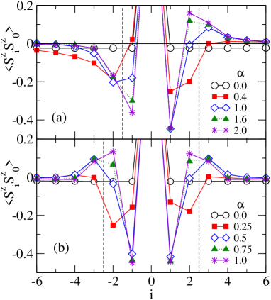
Figure 7: (Color online) Spin correlation functions $\langle S^{z}_{i}S^{z}_{j}\rangle$ between quantum $t_{2g}$ spins (spin-1/2), calculated from the center of the chain at site $j=0$, for the 1D DE model with $J_{\rm H}=32$ and various $\alpha$’s (indicated in the figure) at $T=0$. (a): $L^{(\rm L)}=L^{(\rm R)}=12$ and $L^{(\rm C)}=4$, and the positive background charge densities are $n_{+}^{(\rm L)}$=$n_{+}^{(\rm R)}$=0.5 and $n_{+}^{(\rm C)}$=1.0. (b): $L^{(\rm L)}=L^{(\rm R)}=14$ and $L^{(\rm C)}=5$, and the positive background charge densities are $n_{+}^{(\rm L)}$=$n_{+}^{(\rm R)}$=0.571 and $n_{+}^{(\rm C)}$=1.0. The normalization $\langle S^{z}_{0}S^{z}_{0}\rangle$=$1$ is adopted.

With decreasing $\alpha$, the electron density in the central region is substantially reduced [see Fig. 8 (a)], and eventually the antiferromagnetic correlations at short distances within the central region disappear for both even and odd number of sites in the center (Fig. 7). Together with this effect, an increase in the conductance with decreasing $\alpha$ is observed as shown in Fig. 8 (b). Here the conductance is calculated with the time-dependent DMRG technique tDMRG ; alhassanieh , already explained in Sec. II.2. From these results, in order for the central region to play the role of a tunneling barrier with low conductance, it is clear that the spins in the central region must be antiferromagnetically aligned, and the electronic density there must be close to 1, which is achieved only by a large $\alpha$, i.e., strong Coulomb interactions.

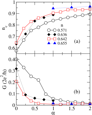
Figure 8: (Color online) (a) Electron density in the central section $n_{c}$ ($=\sum_{i\subset{\rm C}}n_{i}/L^{(\rm C)}$), and (b) conductance $G$, as a function of $\alpha$, for various values of the total electron density $n$ indicated in the plots. Results are for the 1D DE model with quantum $t_{2g}$ spin (spin-1/2) and $J_{\rm H}=32$ at $T=0$, calculated using the DMRG method. The other parameters are $L^{(\rm L)}=L^{(\rm R)}=12$, $L^{(\rm C)}=4$ (circles and squares), $L^{(\rm L)}=L^{(\rm R)}=14$, $L^{(\rm C)}=5$ (diamonds), and $L^{(\rm L)}=L^{(\rm R)}=12$, $L^{(\rm C)}=5$ (triangles). In all cases, the positive background charges are $n_{+}^{(\rm C)}$=1.0 and $n_{+}^{(\rm L)}$=$n_{+}^{(\rm R)}$.

The influence of magnetic fields is also studied in Fig. 9. Here, instead of applying an external magnetic field, the total $z$-component of the spins (i.e., total magnetization), which is a good quantum number of the system, is varied as a parameter. Fig. 9 (a) indicates that the anti-parallel correlations of the lead’s spins, for the case of even number $L^{(\rm C)}=4$ of central sites, becomes parallel with increasing total magnetization. This is in qualitative agreement with the observation in the previous subsection, indicating that classical and quantum $t_{\rm 2g}$ spins behave qualitatively similarly in this system. The same occurs for the case of an odd number of central sites, shown in Fig. 9 (b). There is a small caveat to mention here: (i) the behavior with increasing total magnetization is not monotonous, and (ii) some of the spin correlations in Fig. 9 (as well as in Fig. 7) are small, which might be explained by canting effects or by nearly orthogonal spin configurations. These issues are not further explored here, since they do not appear in the classical $t_{2g}$ spin simulations which seem more realistic to describe manganites. In spite of these caveats, it is clear that qualitatively the similar feature is observed for both models with classical and with quantum $t_{2g}$ spins, the key feature of having anti-parallel magnetic lead configurations for an even number of central sites.

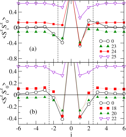
Figure 9: (Color online) Spin correlation functions $\langle S^{z}_{i}S^{z}_{j}\rangle$ between quantum $t_{2g}$ spins (spin-1/2), calculated from the center of the chain at site $j=0$, for the 1D DE model with $J_{\rm H}=32$, $\alpha$=1.0, and various total $S^{z}$ (i.e., total magnetization) indicated in the figure. The calculations are performed with the DMRG method at $T=0$. (a): $L^{(\rm L)}=L^{(\rm R)}=12$, $L^{(\rm C)}=4$, and total electron density $n$=$0.571$. (b): $L^{(\rm L)}=L^{(\rm R)}=12$, $L^{(\rm C)}=5$, and $n$=$0.586$. The positive background charge densities are $n_{+}^{(\rm L)}$=$n_{+}^{(\rm R)}=0.5$ and $n_{+}^{(\rm C)}$=1.0. The normalization $\langle S^{z}_{0}S^{z}_{0}\rangle$=$1$ is adopted.

IV Influence of temperature

The large MR effect at low temperature observed in the trilayer geometry described in this paper is an interesting effect worthy of experimental confirmation. However, for practical applications, this large MR effect should survive up to high temperatures, more specifically room temperature or above. In fact, previous experimental realizations of TMR devices suffered a rapid degradation with increasing temperatures, bowen as mentioned in the introduction (Sec. I.1). Unfortunately, our proposed trilayer system also has problems in this respect, as shown below, but possible avenues to solve this issue are discussed.

In Fig. 10, classical $t_{2g}$ spin correlation functions for two particular sites are shown as a function of temperature $T$, computed with the Monte Carlo technique. One of the chosen sites is in the left lead, site 5, and the other is in the right lead, site 16, and they are symmetrically arranged with respect to the center for the $L=8+4+8$ cluster used. For comparison, the same correlation is shown for the case when the barrier is removed and the entire system is now a unique ferromagnetic metal. yunoki The latter decays with temperature as shown in Fig. 10, indicating that the long-distance ferromagnetic tendencies survive up to $T_{\rm C}\sim$0.03 approximately. Although this should not be considered as a critical temperature, due to the one dimensionality of the problem which introduces strong fluctuations at finite temperatures, at least it provides a good indicator of the strength of ferromagnetism as $T$ is increased. Weak couplings into higher dimensional structures will likely stabilize this characteristic temperature into a true critical temperature. dagotto-CMR ; dagotto-book ; yunoki

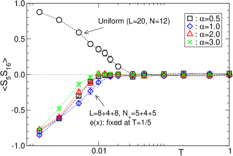
Figure 10: (Color online) Classical $t_{2g}$ spin correlation functions $\langle{\bf S}_{i}\cdot{\bf S}_{j}\rangle$ between site $i$=$5$ (belonging to the left lead) and site $j$=$16$ (belonging to the right lead), as a function of temperature $T$. Monte Carlo simulations are used for the 1D DE model with $J_{\rm H}$=$8.0$, $n_{+}^{(\rm L)}$=$n_{+}^{(\rm R)}$=$0.625$, $n_{+}^{(\rm C)}$=$1.0$, $L^{(\rm L)}$=$L^{(\rm R)}$=$8$, and $L^{(\rm C)}$=$4$. The values of $\alpha$ used are indicated in the figure. Here, $\phi(i)$ is determined self-consistently at $T$=$0.2$ and is subsequently used for other lower temperatures. For comparison, the classical $t_{2g}$ spin correlation functions for a uniform DE model with $J_{\rm H}$=$8.0$, $L$=$20$, and the number of electrons $N$=$12$ are also plotted by circles.

The same spin correlation functions but now in the presence of the barrier is also shown in Fig. 10 for various values of $\alpha$. At low temperatures, these correlation functions have the opposite sign (minus) as compared to the ones without the barrier. This is simply because in this trilayer case there is an even number of sites in the central region, and therefore the magnetic moments between the leads align antiferromagnetically (Sec. III). Here the calculations are carried out by first obtaining the electrostatic potential $\phi(i)$ at high temperature, where the spins are not ordered, and then keeping this potential the same as the temperature is reduced. This procedure considerably alleviates the numerical effort, particularly regarding the Poisson’s equation iterations, and tests in small systems have shown that this trick does not alter the results qualitatively. As also seen in Fig. 10, the spin correlation functions obtained by this method have a relatively minor dependence with $\alpha$. The main point to remark is that these spin correlations become negligible at a temperature $T^{*}\sim 0.01$, which is considerably smaller than the relevant temperature of the pure ferromagnetic system without the barrier. As a consequence, it is clear that a strong similarity with previous experimental results for STO barriers bowen may exist in this case. Expressed qualitatively, our results indicate that there is a temperature scale $T^{*}$, much smaller than the critical temperature $T_{\rm C}$, where the orientation of the leads’ magnetic moments ceases to be antiferromagnetic. As shown below, this is correlated with important changes in the magnetoresistance effect. In fact, the large MR effect at low temperature seems to occur due to the existence of an effective coupling $J_{\rm eff}$ which produces the anti-parallel alignment of the leads’ magnetic moments. This is reasonable, since $J_{\rm eff}$ is an effective weak coupling across a tunneling insulating barrier. When the temperature is of the order of this coupling or larger, the anti-parallel arrangement is no longer preferable and in our model the leads’ moments rotate freely with respect to one another.

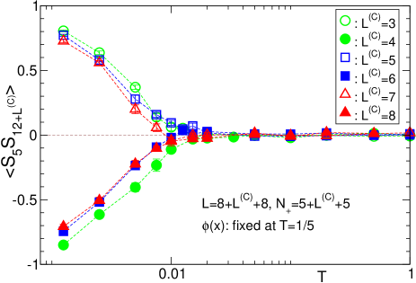
Figure 11: (Color online) Classical $t_{2g}$ spin correlation functions $\langle{\bf S}_{i}\cdot{\bf S}_{j}\rangle$ between sites $i$=$5$ (belonging to the left lead) and site $j$=$12+L^{(\rm C)}$ (belonging to the right lead), for the 1D DE model with $J_{\rm H}$=$8.0$, $\alpha$=$1.0$, $n_{+}^{(\rm L)}$=$n_{+}^{(\rm R)}$=$0.625$, $n_{+}^{(\rm C)}$=$1.0$, $L^{(\rm L)}$=$L^{(\rm R)}$=$8$, and $L^{(\rm C)}$=$3,4,\cdots,8$. Here, $\phi(i)$ is determined self-consistently at $T$=$0.2$ and then used for other temperatures.

A systematic study of the influence of the size of the central region $L^{(\rm C)}$ on the classical $t_{2g}$ spin correlations between the leads is reported in Figure 11. As expected (Sec. I.2), for $L^{(\rm C)}$ even (odd) these spin correlations are negative (positive) at low temperatures, indicating strong antiferromagnetic (ferromagnetic) correlations between the ferromagnetic leads’ moments. The magnitude of this correlation decreases as $L^{(\rm C)}$ increases, in agreement with the expected reduction of the effective coupling $J_{\rm eff}$ discussed above. Thus, the thinner the barrier is, the better the temperature effects become in the trilayer geometry proposed here, namely the higher $T^{*}$ is.

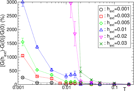
Figure 12: (Color online) Temperature dependence of the MR ratio $[(G(h_{\rm ext})-G(0))/G(0)]\times 100$ for the 1D DE model with $J_{\rm H}$=$8.0$, $\alpha$=$1.0$, $n_{+}^{(\rm L)}$=$n_{+}^{(\rm R)}$=$0.625$, $n_{+}^{(\rm C)}$=$1.0$, $L^{(\rm L)}$=$L^{(\rm R)}$=$8$, and $L^{(\rm C)}$=$4$. Applied magnetic fields $h_{\rm ext}$ are indicated in the figure. $\phi(i)$ is determined self-consistently at $T$=$0.2$ and used for the other temperatures. Note that the effect reported at $T$=0 in Fig. 3 is much larger in magnitude of the order of 200,000% at $h_{\rm ext}$=0.002 (in that figure the factor 100 was not used as in here). In the range of temperatures shown in this figure, the original $T$=0.0 nearly perfect antiferromagnetic alignment of the leads’ magnetic moments is already lost at $h_{\rm ext}$=0, and thus the changes in resistances are not as dramatic as observed at $T=0$.

Our discussion thus far has been based on the spin correlations at finite temperatures. It was concluded that the large resistance caused by the anti-parallel configuration of the ferromagnetic leads’ moments does not survive all the way to the ferromagnetic critical temperatures of the leads. This is indeed observed in Fig. 12, where at $T^{*}$ the MR effect is reduced to zero at fields such as $h_{\rm ext}$=0.001-0.003, while at zero temperature [Fig. 3 (b)] the MR effect was huge at the same fields. However, even though the MR effect is truly enormous at very low temperature, at higher temperatures it is not negligible, at least in the several Teslas scale of magnetic fields $h_{\rm ext}$. For example, in Fig. 12, the MR ratio is plotted vs. temperature, for different values of $h_{\rm ext}$. Note that $[G(h_{\rm ext})-G(0)]/G(0)$ is the same as the more standard definition $[R(0)-R(h_{\rm ext})]/R(h_{\rm ext})$, where the resistance $R(h_{\rm ext})$=$1/G(h_{\rm ext})$. For fields such as $h_{\rm ext}$=0.02 and 0.03 – corresponding to 20 and 30 T, respectively, if it is assumed $t$$\sim$1,000 T – the MR ratio can be as large as 100 or 500% at temperatures of the order of $T_{\rm C}$/2.

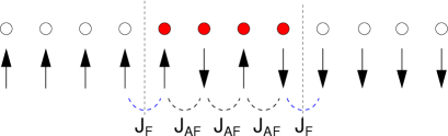
Figure 13: (Color online) Schematic representation of the 1D DE model [Eq. (1)] for a LSMO/LMO/LSMO trilayer (see also Fig. 1) with additional Heisenberg couplings between classical $t_{2g}$ spins, which are introduced to simulate anisotropies. Antiferromagnetic $J_{\rm AF}$, as well as ferromagnetic $J_{\rm F}$, couplings are added only in the central region and the bonds connecting to the central region, as indicated in the figure. The two interface positions are denoted by vertical dashed lines.

In the calculations described so far, no “easy axis” has been chosen. In other words, no anisotropies were introduced. However, the introductory discussion suggests that many materials, particularly when in thin-film form, do have an easy axis mainly due to the influence of the substrate (Sec. I.3). If due to this effect the magnetic moments of the leads cannot rotate “freely” with respect to one another as isotropic Heisenberg vectors, but are pointing along a particular direction as Ising variables, the temperature scale $T^{*}$ above which the magnetic moments of the leads become uncorrelated should increase: Heisenberg-like isotropic spins can be disordered by thermal fluctuations more easily than Ising-like spins. On the other hand, making more “rigid” the anti-parallel magnetic connection between the leads moments will also prevent their alignment in very small magnetic fields: larger magnetic fields may be needed to achieve the same effect as before, i.e., large MR effect. These competing tendencies will be discussed in more detail below.

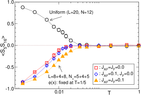
Figure 14: (Color online) Classical $t_{2g}$ spin correlation functions $\langle{\bf S}_{i}\cdot{\bf S}_{j}\rangle$ between site $i=5$ (belonging to the left lead) and site $j=16$ (belonging to the right lead), as a function of temperature $T$. Monte Carlo simulations are used for the 1D DE model with $J_{\rm H}$=$8.0$ and $\alpha=1.0$. The positive background charge densities are $n_{+}^{(\rm L)}$=$n_{+}^{(\rm R)}=0.625$ and $n_{+}^{(\rm C)}=1.0$, and the cluster used is $L^{(\rm L)}=L^{(\rm R)}=8$ and $L^{(\rm C)}=4$. The results with $J_{\rm AF}=J_{\rm F}=0.1$ are shown by triangles, and the results with $J_{\rm AF}=0.1$ but no $J_{\rm F}$ are denoted by diamonds. For comparison, the results for a uniform DE model without the barrier (circles) and the results with the central barrier but no $J_{\rm AF}$ and $J_{\rm F}$ (squares) are also plotted. These are reproduced from Fig. 10. Note that with nonzero $J_{\rm F}$ and $J_{\rm AF}$, the spin correlations now vanish at almost the same temperature as in the case without the barrier (circles). Here, $\phi(i)$ is determined self-consistently at $T$=$0.2$ and is subsequently used for other lower temperatures.

To investigate this issue, extra couplings between classical $t_{2g}$ spins are added to the model, as shown in Fig. 13. Via direct Heisenberg couplings between the classical spins, $J_{\rm AF}$ (antiferromagnetic) and $J_{\rm F}$ (ferromagnetic), both the antiferromagnetic spin arrangement in the central region and the coupling between the center and the leads can be made more rigid. That this procedure helps regarding the $T^{*}$ problem is clear in Fig. 14 where the classical $t_{2g}$-spin correlation functions are shown. Contrary to the case of weakly coupled leads, now a robust spin correlation between them survives up to $T_{\rm C}$. However, the MR effect is not improving at very small fields (see Fig. 15). On the contrary, larger values of $h_{\rm ext}$ are needed to achieve the same MR effect as before (for instance, the MR ratio at $h_{\rm ext}$=0.01 without anisotropies is 3000% at $T$$\sim$0.001, while it is 1500% here with anisotropy). Thus, as already mentioned briefly, the overall conclusion is that there are two competing tendencies to consider in these investigations: (i) on one hand, a weak coupling among the leads, mediated by the central region, is needed in order for a tiny magnetic field to cause a huge effect in transport; (ii) on the other hand, for the same reason, a small temperature can entirely wash out the effect. Adding anisotropies increases the effective coupling between the leads’ magnetic moments, thus helping with the temperature issue (ii), but reciprocally, larger magnetic fields are needed to achieve the same MR effect. Investigating the subtle balance between these competing tendencies is a great challenge, both for theorists and experimentalists.

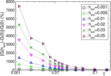
Figure 15: (Color online) The same as in Fig. 12 except that additional couplings between the classical $t_{2g}$ spins, $J_{\rm AF}$=$J_{\rm F}$=$0.1$, are added to simulate the presence of anisotropies (see Fig. 13). The applied magnetic fields $h_{\rm ext}$ are indicated in the figure. The electrostatic potential $\phi(i)$ is determined self-consistently at $T$=$0.2$ and then used for other lower temperatures.

V Ti-oxide barrier

Although the focus of our effort has been on the LSMO/LMO/LSMO trilayer, as mentioned in the introduction we have also carried out model Hamiltonian simulations for the more standard case of a non-magnetic insulator as a barrier. A widely studied material for this purpose is STO, which is here mimicked simply by a tight-binding Hamiltonian for the barrier, with its energy levels shifted by a one-particle site potential $V_{\rm m}$ which controls the height of the barrier. In this section, results for the case LSMO/STO/LSMO are briefly discussed, with the emphasis on qualitative aspects and comparisons with the case of LMO as barrier. The details of the model Hamiltonian were already described in Sec. II, and the technique employed is the MC simulation. Once again, it should be remarked that subtle effects such as “dead layers” are not considered in this study (Sec. I.3), and their presence may affect quantitatively our conclusions.

The local electronic density $n(i)$ is reported in Fig. 16 for the 1D LSMO/STO/LSMO model with different values of the site potential $V_{\rm m}$ in the central region. It is observed that $n(i)$ in the central region gradually increases from nearly zero to $\sim 0.4$ with decreasing $V_{\rm m}$, indicating that the barrier hight decreases with $V_{\rm m}$, and consequently the effective coupling between the leads becomes stronger. Note that the lower band of the lead (described by the DE model) is centered at $-J_{\rm H}$, and thus the band of the central region and the lower band of the lead are perfectly aligned (i.e., zero barrier height) when $V_{\rm m}=-J_{\rm H}$ (and $\alpha=0$).

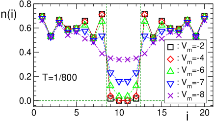
Figure 16: (Color online) Electron density $n(i)$ for the 1D LSMO/STO/LSMO model (see the text) with $J_{\rm H}=8.0$ and $\alpha=1.0$, at $T=1/800$, and for various values of $V_{\rm m}$ (indicated in the figure). The positive background charges are $n_{+}^{(\rm L)}$=$n_{+}^{(\rm R)}$=$0.625$ and $n_{+}^{(\rm C)}$=$0.0$, and the system size studied is $L^{(\rm L)}$=$L^{(\rm R)}$=$8$ and $L^{(\rm C)}$=$4$. The positions of the two interfaces are denoted by vertical dashed lines. The electrostatic potential $\phi(i)$ is determined self-consistently.

In Fig. 17, the MR ratio vs. temperature for the case $V_{\rm m}=-7.0$ is shown. Notice that the MR effect becomes appreciable at temperatures comparable to the Curie temperature of the individual ferromagnetic leads. This is qualitatively similar to the effect observed in LSMO/LMO/LSMO for the case where an anisotropy was introduced (Fig. 15), which effectively caused a stronger effective coupling between the magnetic moments of the left and right leads. Thus, it appears that the value $V_{\rm m}=-7.0$ chosen for this example allows for a robust left-right coupling (as also expected from $n(i)$ shown in Fig. 16), concomitant with the survival of a large MR effect up to the Curie temperature. It is also observed in Fig. 17 that because of the strong effective coupling between the leads, the MR ratio for small magnetic fields ($\lesssim 0.003$) is not as large as in the case of the small effective coupling discussed below (Fig. 18).

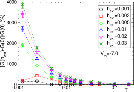
Figure 17: (Color online) MR ratio $[G(h_{\rm ext})-G(0)]/G(0)\times 100$ vs. temperature $T$ for the 1D LSMO/STO/LSMO model (see the text) with $J_{\rm H}=8.0$, $\alpha=1.0$, and $V_{\rm m}=-7.0$. The positive background charges are $n_{+}^{(\rm L)}$=$n_{+}^{(\rm R)}$=$0.625$ and $n_{+}^{(\rm C)}$=$0.0$, and the system size studied is $L^{(\rm L)}$=$L^{(\rm R)}$=$8$ and $L^{(\rm C)}$=$4$. Applied magnetic fields $h_{\rm ext}$ are indicated in the figure. Here, $\phi(i)$ is determined self-consistently for all temperatures.

Figure 18 shows results for the same parameters as in Fig. 17, but simply making the height of the barrier $V_{\rm m}$ much larger, i.e., the left and right leads being nearly decoupled. Three effects are obvious to the eye: (i) the large MR effect appears now at lower temperatures. For example, in Fig. 18 the MR becomes nonzero at T$\sim$0.02, while in Fig. 17 the same occurred at a higher temperature $\sim 0.03-0.04$. (ii) On the other hand, increasing the height of the barrier much increases the MR ratio at low temperatures and small magnetic fields. For example, in Fig. 18 the MR ratio is about 1,000% at T$\sim$0.001 and $h_{\rm ext}=0.001$, while in Fig. 17 it is about 200% at the same $T$ and $h_{\rm ext}$. This occurs because the barrier is so large in Fig. 18 that in the absence of magnetic fields, the magnetic moments of the left and right leads are almost decoupled, and thus applying a very small magnetic field is enough to align the leads’ magnetic moment and increase conductance. (iii) The dependence of magnetic fields on the MR ratio is very mild (compared to Fig. 17), namely changing $h_{\rm ext}$ from 0.001 to 0.03 only alters the results by a factor 2 at the most. This is because the almost decoupled leads moments are forced to align in the magnetic field direction by a very small $h_{\rm ext}$. A further increase of $h_{\rm ext}$ does not change the moments orientation at low temperatures.

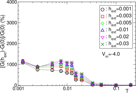
Figure 18: (Color online) The same as in Fig. 17, except that $V_{\rm m}$=$-4.0$.

Thus, an interesting and simple picture emerges from these qualitative investigations, which are in agreement with the results shown before for the case of LSMO/LMO/LSMO: (1) If the barrier between the magnetic leads is very large (i.e., the effective coupling between the leads is small), the magnetic moments of the ferromagnetic leads are nearly decoupled (in the absence of anisotropies) at $h_{\rm ext}$=0, even at low temperatures. Thus, the double effect of large barrier and concomitant weakly coupled leads causes a large $h_{\rm ext}$=0 resistance, which enhances the MR effect at low temperatures as compared with a lower barrier (i.e., the large effective coupling between the leads). (2) However, the large barrier and weakly coupled leads are fragile upon increasing the temperature.

VI Conclusions

In this paper, the use of LSMO/LMO/LSMO as a spin-tunnel-junction is proposed. The main difference with other previous efforts is in the use of a manganite barrier. This would improve the lattice spacing matching between the constituents, hopefully also alleviating the complications found in previous investigations such as the infamous interfacial dead layers of STO/LSMO. However, the main point of this study is not just the all-manganite character of the trilayer, but the antiferromagnetic properties of LMO. For an even number of LMO layers, the spin order in the ground state is such that the magnetic moments of the ferromagnetic LSMO leads are anti-parallel (while for an odd number of layers, they are parallel). An anti-parallel-leads configuration has a large resistance. But the effective coupling leading to this anti-parallel LSMO-moments configuration is weak, rendering the ground state fragile. In fact, numerical simulations show that very small magnetic fields $h_{\rm ext}$ can alter drastically the original ground state at $h_{\rm ext}=0$, by aligning the magnetic moments of the ferromagnetic LSMO leads. A very large MR effect is observed in this transition, at least at low temperatures. Note that in arriving to our conclusions a large number of approximations have been made, all clearly described in Sec. I.3. However, we still expect that our theoretical analysis is qualitatively correct and may serve as a motivation for a real experimental realization of the LSMO/LMO/LSMO magnetic junction.

Other effects, such as the influence of temperature, were also considered in this study. Together with the analysis of STO as barrier, overall trends were identified. Very insulating barriers (inducing a very week effective coupling between the leads) can lead to low-temperature states which are easily destabilized by small magnetic fields, causing a large MR effect. However, thermal fluctuation rapidly washes out these large effects. Reducing the barrier height or introducing anisotropies make the original ground state at $h_{\rm ext}=0$ more robust with increasing temperature, but this reduces the low-temperature MR effect at small magnetic fields. A balance between these two tendencies is needed to find optimal trilayers for real devices.

Note added: While completing the work described in this paper, we received two preprints with interesting related efforts: (1) Salafranca et al. salafranca have reported a theoretical study of an all-manganite heterostructure consisting of FM electrodes and an AF barrier, similar in spirit to ours. However, contrary to our proposed system, the chosen barrier salafranca is Pr_2/3Ca_1/3MnO₃, which has CE-type ordering and the same hole doping as the electrodes, which were chosen to be LSMO with $x$=1/3. The emphasis of Ref. salafranca, is not on differences between even and odd number of central layers as in the present paper, but on other interesting effects such as the influence of the FM electrodes on the spin arrangement of the barrier. Thus, Ref. salafranca, and our efforts nicely complement each other. (2) Yu et al.yu have presented experimental results for an all-manganite trilayer using LSMO $x$=0.3 as electrodes and LSMO $x$=0.04 as barrier (the latter being almost identical to the LMO barrier theoretically proposed in this paper). Those authors report a huge TMR ratio of 30,000% at 4.2 K and with bias voltage 25 mV (our MR ratio is 200,000% at $h_{\rm ext}$=0.001). The barrier thickness is 9 atomic layers. Yu et al. assign the large MR effect they observed to thermally activated magnon resonances inside the barrier. A detail comparison between theory and experiment will be carried out in the near future.

- (1) E. Dagotto, T. Hotta, and A. Moreo, Physics Reports 344, 1 (2001), and references therein. See also E. Dagotto, Science 309, 257 (2005), and references therein.
- (2) A. Ohtomo, D. A. Muller, J. L. Grazul, and H. Y. Hwang, Nature 419, 378 (2002); A. Ohtomo and H. Y. Hwang, Nature 427, 423 (2004); S. Okamoto and A. Millis, Nature 428, 630 (2004); S. Okamoto, A. J. Millis, and N. A. Spaldin, Phys. Rev. Lett. 97, 056802 (2006); N. Nakagawa, H. Y. Hwang, and D. A. Muller, Nature Materials 5, 204 (2006); S. Thiel, G. Hammerl, A. Schmehl, C. W. Schneider, and J. Mannhart, Science 313, 1942 (2006); J. Chakhalian, J. W. Freeland, H.-U. Habermeier, G. Cristiani, G. Khaliullin, M. van Veenendaal, and B. Keimer, Science 318, 1114 (2007); E. Dagotto, Science 318, 1076 (2007); and references therein.
- (3) J. Moodera, L. Kinder, T. Wong, and R. Meservey, Phys. Rev. Lett. 74, 3273 (1995).
- (4) For reviews considering manganite tunnel structures see J. M. Coey, M. Viret, and S. von Molnár, Adv. Phys. 48, 167 (1999); M. Ziese, Rep. Prog. Phys. 65, 143 (2002); K. Dörr, J. Phys. D: Appl. Phys. 39, R125 (2006); M. Bibes and A. Barthélémy, arXiv:0706.3015.
- (5) J. Park, E. Vescovo, H. Kim, C. Kwon, R. Ramesh, and T. Venkatesan, Nature 392, 794 (1998).
- (6) M. Bowen, M. Bibes, A. Berthélémy, J-P. Contour, A. Anane, Y. Lemaitre, and A. Fert, App. Phys. Lett. 82, 233 (2003), and references. therein.
- (7) H. Yamada, Y. Ogawa, Y. Ishii, H. Sato, M. Kawasaki, H. Akoh, and Y. Tokura, Science 305, 646 (2004), and references therein. See also Y. Ishii, H. Yamada, H. Sato, H. Akoh, Y. Ogawa, M. Kawasaki, and Y. Tokura, App. Phys. Lett. 89, 042509 (2006).
- (8) To our knowledge, LMO was not experimentally used as a barrier in tunnel junctions before. However, in M-H. Jo, M. Blamire, D. Ozkaya, and A. Petford-Long, J. Phys.: Condens. Matter 15, 5243 (2003), results for the case LCMO(0.3)/LCMO(0.55)/LCMO(0.3) were reported. Here LCMO() is La1-xCaxMnO3. The case =0.55 corresponds to a CE-like state that has charge, orbital, and spin order. dagotto-CMR
- (9) M. Mathews, F. Postma, J. Cock Lodder, R. Jansen, G. Rijnders, and D. Blank, Appl. Phys. Lett. 87, 242507 (2005).
- (10) Y. Ishii, H. Yamada, H. Sato, H. Akoh, M. Kawasaki, and Y. Tokura, Appl. Phys. Lett. 87, 022509 (2005) and references therein.
- (11) See, for example, S. Datta, Electronic transport in mesoscopic systems (Cambridge University Press, Cambridge, 1997).
- (12) S. Yunoki, J. Hu, A. L. Malvezzi, A. Moreo, N. Furukawa, and E. Dagotto, Phys. Rev. Lett. 80, 845 (1998); S. Yunoki and A. Moreo, Phys. Rev. B 58, 6403 (1998); E. Dagotto, S. Yunoki, A. L. Malvezzi, A. Moreo, J. Hu, S. Capponi, D. Poilblanc, and N. Furukawa, Phys. Rev. B 58, 6414 (1998).
- (13) W. H. Press, S. A. Teukolsky, W. T. Vetterling, and B. P. Flannery, Numerical Recipes (Cambridge University Press, Cambridge, 1992).
- (14) J. A. Vergés, Comput. Phys. Commun. 118, 71 (1999).
- (15) E. Dagotto, Nanoscale Phase Separation and Colossal Magnetoresistance (Springer Verlag, Berlin, 2002).
- (16) A. Sawa, A. Yamamoto, H. Yamada, T. Fujii, M. Kawasaki, J. Matsuno, and Y. Tokura, Appl. Phys. Lett. 90, 252102 (2007).
- (17) S. Yunoki, A. Moreo, E. Dagotto, S. Okamoto, S. S. Kancharla, and A. Fujimori, Phys. Rev. B 76, 064532 (2007).
- (18) S. R. White, Phys. Rev. Lett. 69, 2863 (1992); K. Hallberg, Adv. Phys. 55, 477 (2006); U. Schollwöck, Rev. Mod. Phys. 77, 259 (2005).
- (19) S. Costamagna, C. J. Gazza, M. E. Torio, and J. A. Riera, Phys. Rev. B 74, 195103 (2006).
- (20) S. White and A. Feiguin, Phys. Rev. Lett. 93, 076401 (2004).
- (21) K. A. Al-Hassanieh, A. E. Feiguin, J. A. Riera, C. A. Büsser, and E. Dagotto, Phys. Rev. B 73, 195304 (2006).
- (22) C. Zener, Phys. Rev. 82, 403 (1951); P. W. Anderson and H. Hasegawa, Phys. Rev. 100, 675 (1955); P. G. de Gennes, Phys. Rev. 118, 141 (1960).
- (23) C. Sen, G. Alvarez, and E. Dagotto, Phys. Rev. Lett. 98, 127202 (2007).
- (24) J. Salafranca, M. J. Calderón, and L. Brey, arXiv:0709.3720.
- (25) D. B. Yu, J. F. Feng, Y. Wang, X. F. Han, Y. S. Du, H. Yan, Z. Zhang, G. C. Zhang, X.-G. Zhang, S. van Dijken, and J. M. D. Coey, preprint, 2007.