Data-driven Calibration of Penalties for Least-Squares Regression

Abstract

Penalization procedures often suffer from their dependence on multiplying factors, whose optimal values are either unknown or hard to estimate from data. We propose a completely data-driven calibration algorithm for these parameters in the least-squares regression framework, without assuming a particular shape for the penalty. Our algorithm relies on the concept of minimal penalty, recently introduced by Birgé and Massart (2007) in the context of penalized least squares for Gaussian homoscedastic regression. On the positive side, the minimal penalty can be evaluated from the data themselves, leading to a data-driven estimation of an optimal penalty which can be used in practice; on the negative side, their approach heavily relies on the homoscedastic Gaussian nature of their stochastic framework.

The purpose of this paper is twofold: stating a more general heuristics for designing a data-driven penalty (the slope heuristics) and proving that it works for penalized least-squares regression with a random design, even for heteroscedastic non-Gaussian data. For technical reasons, some exact mathematical results will be proved only for regressogram bin-width selection. This is at least a first step towards further results, since the approach and the method that we use are indeed general.

Keywords: Data-driven Calibration, Non-parametric Regression, Model Selection by Penalization, Heteroscedastic Data, Regressogram

1 Introduction

In the last decades, model selection has received much interest, commonly through penalization. In short, penalization chooses the model minimizing the sum of the empirical risk (how well the algorithm fits the data) and of some measure of complexity of the model (called penalty); see FPE (Akaike, 1970), AIC (Akaike, 1973), Mallows’ $C_{p}$ or $C_{L}$ (Mallows, 1973). Many other penalization procedures have been proposed since, among which Rademacher complexities (Koltchinskii, 2001; Bartlett et al., 2002), local Rademacher complexities (Bartlett et al., 2005; Koltchinskii, 2006), bootstrap penalties (Efron, 1983), resampling and $V$-fold penalties (Arlot, 2008b, c).

Model selection can target two different goals. On the one hand, a procedure is efficient (or asymptotically optimal) when its quadratic risk is asymptotically equivalent to the risk of the oracle. On the other hand, a procedure is consistent when it chooses the smallest true model asymptotically with probability one. This paper deals with efficient procedures, without assuming the existence of a true model.

A huge amount of literature exists about efficiency. First Mallows’ $C_{p}$, Akaike’s FPE and AIC are asymptotically optimal, as proved by Shibata (1981) for Gaussian errors, by Li (1987) under suitable moment assumptions on the errors, and by Polyak and Tsybakov (1990) under sharper moment conditions, in the Fourier case. Non-asymptotic oracle inequalities (with some leading constant $C>1$) have been obtained by Barron et al. (1999) and by Birgé and Massart (2001) in the Gaussian case, and by Baraud (2000, 2002) under some moment assumptions on the errors. In the Gaussian case, non-asymptotic oracle inequalities with leading constant $C_{n}$ tending to 1 when $n$ tends to infinity have been obtained by Birgé and Massart (2007).

However, from the practical point of view, both AIC and Mallows’ $C_{p}$ still present serious drawbacks. On the one hand, AIC relies on a strong asymptotic assumption, so that for small sample sizes, the optimal multiplying factor can be quite different from one. Therefore, corrected versions of AIC have been proposed (Sugiura, 1978; Hurvich and Tsai, 1989). On the other hand, the optimal calibration of Mallows’ $C_{p}$ requires the knowledge of the noise level $\sigma^{2}$, assumed to be constant. When real data are involved, $\sigma^{2}$ has to be estimated separately and independently from any model, which is a difficult task. Moreover, the best estimator of $\sigma^{2}$ (say, with respect to the quadratic error) quite unlikely leads to the most efficient model selection procedure. Contrary to Mallows’ $C_{p}$, the data-dependent calibration rule defined in this article is not a “plug-in” method; it focuses directly on efficiency, which can improve significantly the performance of the model selection procedure.

Existing penalization procedures present similar or stronger drawbacks than AIC and Mallows’ $C_{p}$, often because of a gap between theory and practice. For instance, oracle inequalities have only been proved for (global) Rademacher penalties multiplied by a factor two (Koltchinskii, 2001), while they are used without this factor (Lozano, 2000). As proved by Arlot (2007, Chapter 9), this factor is necessary in general. Therefore, the optimal calibration of these penalties is really an issue. The calibration problem is even harder for local Rademacher complexities: theoretical results hold only with large calibration constants, particularly the multiplying factor, and no optimal values are known. One of the purposes of this paper is to address the issue of optimizing the multiplying factor for general-shape penalties.

Few automatic calibration algorithms are available. The most popular ones are certainly cross-validation methods (Allen, 1974; Stone, 1974), in particular $V$-fold cross-validation (Geisser, 1975), because these are general-purpose methods, relying on a widely valid heuristics. However, their computational cost can be high. For instance, $V$-fold cross-validation requires the entire model selection procedure to be performed $V$ times for each candidate value of the constant to be calibrated. For penalties proportional to the dimension of the models, such as Mallows’ $C_{p}$, alternative calibration procedures have been proposed by George and Foster (2000) and by Shen and Ye (2002).

A completely different approach has been proposed by Birgé and Massart (2007) for calibrating dimensionality-based penalties. Since this article extends their approach to a much wider range of applications, let us briefly recall their main results. In Gaussian homoscedastic regression with a fixed design, assume that each model is a finite-dimensional vector space. Consider the penalty $\operatorname{pen}(m)=KD_{m}$, where $D_{m}$ is the dimension of the model $m$ and $K>0$ is a positive constant, to be calibrated. First, there exists a minimal constant $K_{\min}$, such that the ratio between the quadratic risk of the chosen estimator and the quadratic risk of the oracle is asymptotically infinite if $K<K_{\min}$, and finite if $K>K_{\min}$. Second, when $K=K^{\star}:=2K_{\min}$, the penalty $KD_{m}$ yields an efficient model selection procedure. In other words, the optimal penalty is twice the minimal penalty. This relationship characterizes the “slope heuristics” of Birgé and Massart (2007).

A crucial fact is that the minimal constant $K_{\min}$ can be estimated from the data, since large models are selected if and only if $K<K_{\min}$. This leads to the following strategy for choosing $K$ from the data. For every $K\geq 0$, let $\widehat{m}(K)$ be the model selected by minimizing the empirical risk penalized by $\operatorname{pen}(D_{m})=KD_{m}$. First, compute $K_{\min}$ such that $D_{\widehat{m}(K)}$ is “huge” for $K<K_{\min}$ and “reasonably small” when $K\geq K_{\min}$; explicit values for “huge” and “small” are proposed in Section 3.3. Second, define $\widehat{m}:=\widehat{m}(2K_{\min})$. Such a method has been successfully applied for multiple change points detection by Lebarbier (2005).

From the theoretical point of view, the issue for understanding and validating this approach is the existence of a minimal penalty. This question has been addressed for Gaussian homoscedastic regression with a fixed design by Birgé and Massart (2001, 2007) when the variance is known, and by Baraud et al. (2007) when the variance is unknown. Non-Gaussian or heteroscedastic data have never been considered. This article contributes to fill this gap in the theoretical understanding of penalization procedures.

The calibration algorithm proposed in this article relies on a generalization of Birgé and Massart’s slope heuristics (Section 2.3). In Section 3, the algorithm is defined in the least-squares regression framework, for general-shape penalties. The shape of the penalty itself can be estimated from the data, as explained in Section 3.4.

The theoretical validation of the algorithm is provided in Section 4, from the non-asymptotic point of view. Non-asymptotic means in particular that the collection of models is allowed to depend on $n$: in practice, it is usual to allow the number of explanatory variables to increase with the number of observations. Considering models with a large number of parameters (for example of the order of a power of the sample size $n$) is also necessary to approximate functions belonging to a general approximation space. Thus, the non-asymptotic point of view allows us not to assume that the regression function is described with a small number of parameters.

The existence of minimal penalties for heteroscedatic regression with a random design (Theorem 2) is proved in Section 4.3. In Section 4.4, by proving that twice the minimal penalty has some optimality properties (Theorem 3), we extend the so-called slope heuristics to heteroscedatic regression with a random design. Moreover, neither Theorem 2 nor Theorem 3 assume the data to be Gaussian; only mild moment assumptions are required.

For proving Theorems 2 and 3, each model is assumed to be the vector space of piecewise constant functions on some partition of the feature space. This is indeed a restriction, but we conjecture that it is mainly technical, and that the slope heuristics remains valid at least in the general least-squares regression framework. We provide some evidence for this by proving two key concentration inequalities without the restriction to piecewise constant functions. Another argument supporting this conjecture is that recently several simulation studies have shown that the slope heuristics can be used in several frameworks: mixture models (Maugis and Michel, 2008), clustering (Baudry, 2007), spatial statistics (Verzelen, 2008), estimation of oil reserves (Lepez, 2002) and genomics (Villers, 2007). Although the slope heuristics has not been formally validated in these frameworks, this article is a first step towards such a validation, by proving that the slope heuristics can be applied whatever the shape of the ideal penalty.

This paper is organized as follows. The framework and the slope heuristics are described in Section 2. The resulting algorithm is defined in Section 3. The main theoretical results are stated in Section 4. All the proofs are given in Appendix A.

2 Framework

In this section, we describe the framework and the general slope heuristics.

2.1 Least-squares regression

Suppose we observe some data $(X_{1},Y_{1}),\ldots(X_{n},Y_{n})\in\mathcal{X}\times\mathbb{R}$, independent with common distribution $P$, where the feature space $\mathcal{X}$ is typically a compact set of $\mathbb{R}^{d}$. The goal is to predict $Y$ given $X$, where $(X,Y)\sim P$ is a new data point independent of $(X_{i},Y_{i})_{1\leq i\leq n}$. Denoting by $s$ the regression function, that is $s(x)=\mathbb{E}\left[\left.Y\,\right|\left.\,X=x\right.\right]$ for every $x\in\mathcal{X}$, we can write

$$Y_{i}=s(X_{i})+\sigma(X_{i})\epsilon_{i}$$ (1)

where $\sigma:\mathcal{X}\mapsto\mathbb{R}$ is the heteroscedastic noise level and $\epsilon_{i}$ are i.i.d. centered noise terms, possibly dependent on $X_{i}$, but with mean 0 and variance 1 conditionally to $X_{i}$.

The quality of a predictor $t:\mathcal{X}\mapsto\mathcal{Y}$ is measured by the (quadratic) prediction loss

$$\mathbb{E}_{(X,Y)\sim P}\left[\left.\gamma(t,(X,Y))\right.\right]=:P\gamma(t)\qquad\mbox{where}\quad\gamma(t,(x,y))=\left(\left.t(x)-y\right.\right)^{2}$$

is the least-squares contrast. The minimizer of $P\gamma(t)$ over the set of all predictors, called Bayes predictor, is the regression function $s$. Therefore, the excess loss is defined as

$$\ell\left(\left.s,t\right.\right):=P\gamma\left(\left.t\right.\right)-P\gamma\left(\left.s\right.\right)=\mathbb{E}_{(X,Y)\sim P}\left(t(X)-s(X)\right)^{2}\enspace.$$

Given a particular set of predictors $S_{m}$ (called a model), we define the best predictor over $S_{m}$ as

$$s_{m}:=\arg\min_{t\in S_{m}}\left\{\left.P\gamma(t)\right.\right\}\enspace,$$

with its empirical counterpart

$$\widehat{s}_{m}:=\arg\min_{t\in S_{m}}\left\{\left.P_{n}\gamma(t)\right.\right\}$$

(when it exists and is unique), where $P_{n}=n^{-1}\sum_{i=1}^{n}\delta_{(X_{i},Y_{i})}$. This estimator is the well-known empirical risk minimizer, also called least-squares estimator since $\gamma$ is the least-squares contrast.

2.2 Ideal model selection

Let us assume that we are given a family of models $(S_{m})_{m\in\mathcal{M}_{n}}$, hence a family of estimators $(\widehat{s}_{m})_{m\in\mathcal{M}_{n}}$ obtained by empirical risk minimization. The model selection problem consists in looking for some data-dependent $\widehat{m}\in\mathcal{M}_{n}$ such that $\ell\left(\left.s,\widehat{s}_{\widehat{m}}\right.\right)$ is as small as possible. For instance, it would be convenient to prove some oracle inequality of the form

$$\ell\left(\left.s,\widehat{s}_{\widehat{m}}\right.\right)\leq C\inf_{m\in\mathcal{M}_{n}}\left\{\left.\ell\left(\left.s,\widehat{s}_{m}\right.\right)\right.\right\}+R_{n}$$

in expectation or on an event of large probability, with leading constant $C$ close to 1 and $R_{n}=o(n^{-1})$.

General penalization procedures can be described as follows. Let $\operatorname{pen}:\mathcal{M}_{n}\mapsto\mathbb{R}^{+}$ be some penalty function, possibly data-dependent, and define

$$\widehat{m}\in\arg\min_{m\in\mathcal{M}_{n}}\left\{\left.\operatorname{crit}(m)\right.\right\}\qquad\mbox{with}\qquad\operatorname{crit}(m):=P_{n}\gamma(\widehat{s}_{m})+\operatorname{pen}(m)\enspace.$$ (2)

Since the ideal criterion $\operatorname{crit}(m)$ is the true prediction error $P\gamma\left(\left.\widehat{s}_{m}\right.\right)$, the ideal penalty is

$$\operatorname{pen}_{\mathrm{id}}(m):=P\gamma(\widehat{s}_{m})-P_{n}\gamma(\widehat{s}_{m})\enspace.$$

This quantity is unknown because it depends on the true distribution $P$. A natural idea is to choose $\operatorname{pen}(m)$ as close as possible to $\operatorname{pen}_{\mathrm{id}}(m)$ for every $m\in\mathcal{M}_{n}$. We will show below, in a general setting, that when $\operatorname{pen}$ is a good estimator of the ideal penalty $\operatorname{pen}_{\mathrm{id}}$, then $\widehat{m}$ satisfies an oracle inequality with leading constant $C$ close to 1.

By definition of $\widehat{m}$,

$$\forall m\in\mathcal{M}_{n},\quad P_{n}\gamma(\widehat{s}_{\widehat{m}})\leq P_{n}\gamma(\widehat{s}_{m})+\operatorname{pen}(m)-\operatorname{pen}(\widehat{m})\enspace.$$

For every $m\in\mathcal{M}_{n}$, we define

$$p_{1}(m)=P\left(\left.\gamma(\widehat{s}_{m})-\gamma(s_{m})\right.\right)\quad p_{2}(m)=P_{n}\left(\left.\gamma(s_{m})-\gamma(\widehat{s}_{m})\right.\right)\quad\delta(m)=(P_{n}-P)\left(\left.\gamma(s_{m})\right.\right)$$

so that

$$\operatorname{pen}_{\mathrm{id}}(m)=p_{1}(m)+p_{2}(m)-\delta(m)$$

$$\mbox{and}\qquad\ell\left(\left.s,\widehat{s}_{m}\right.\right)=P_{n}\gamma(\widehat{s}_{m})+p_{1}(m)+p_{2}(m)-\delta(m)-P\gamma(s)\enspace.$$

Hence, for every $m\in\mathcal{M}_{n}$,

$$\ell\left(\left.s,\widehat{s}_{\widehat{m}}\right.\right)+(\operatorname{pen}-\operatorname{pen}_{\mathrm{id}})(\widehat{m})\leq\ell\left(\left.s,\widehat{s}_{m}\right.\right)+(\operatorname{pen}-\operatorname{pen}_{\mathrm{id}})(m)\enspace.$$ (3)

Therefore, in order to derive an oracle inequality from (3), it is sufficient to show that for every $m\in\mathcal{M}_{n}$, $\operatorname{pen}(m)$ is close to $\operatorname{pen}_{\mathrm{id}}(m)$.

2.3 The slope heuristics

If the penalty is too big, the left-hand side of (3) is larger than $\ell\left(\left.s,\widehat{s}_{\widehat{m}}\right.\right)$ so that (3) implies an oracle inequality, possibly with large leading constant $C$. On the contrary, if the penalty is too small, the left-hand side of (3) may become negligible with respect to $\ell\left(\left.s,\widehat{s}_{\widehat{m}}\right.\right)$ (which would make $C$ explode) or—worse—may be nonpositive. In the latter case, no oracle inequality may be derived from (3). We shall see in the following that $\ell\left(\left.s,\widehat{s}_{\widehat{m}}\right.\right)$ blows up if and only if the penalty is smaller than some “minimal penalty”.

Let us consider first the case $\operatorname{pen}(m)=p_{2}(m)$ in (2). Then, $\mathbb{E}\left[\left.\operatorname{crit}(m)\right.\right]=\mathbb{E}\left[\left.P_{n}\gamma\left(\left.s_{m}\right.\right)\right.\right]=P\gamma\left(\left.s_{m}\right.\right)$, so that $\widehat{m}$ approximately minimizes its bias. Therefore, $\widehat{m}$ is one of the more complex models, and the risk of $\widehat{s}_{\widehat{m}}$ is large. Let us assume now that $\operatorname{pen}(m)=Kp_{2}(m)$. If $0<K<1$, $\operatorname{crit}(m)$ is a decreasing function of the complexity of $m$, so that $\widehat{m}$ is again one of the more complex models. On the contrary, if $K>1$, $\operatorname{crit}(m)$ increases with the complexity of $m$ (at least for the largest models), so that $\widehat{m}$ has a small or medium complexity. This argument supports the conjecture that the “minimal amount of penalty” required for the model selection procedure to work is $p_{2}(m)$.

In many frameworks such as the one of Section 4.1, it turns out that

$$\forall m\in\mathcal{M}_{n},\qquad p_{1}(m)\approx p_{2}(m)\enspace.$$

Hence, the ideal penalty $\operatorname{pen}_{\mathrm{id}}(m)\approx p_{1}(m)+p_{2}(m)$ is close to $2p_{2}(m)$. Since $p_{2}(m)$ is a “minimal penalty”, the optimal penalty is close to twice the minimal penalty:

$$\operatorname{pen}_{\mathrm{id}}(m)\approx 2\operatorname{pen}_{\min}(m)\enspace.$$

This is the so-called “slope heuristics”, first introduced by Birgé and Massart (2007) in a Gaussian homoscedastic setting. Note that a formal proof of the validity of the slope heuristics has only been given for Gaussian homoscedastic least-squares regression with a fixed design (Birgé and Massart, 2007); up to the best of our knowledge, the present paper yields the second theoretical result on the slope heuristics.

This heuristics has some applications because the minimal penalty can be estimated from the data. Indeed, when the penalty smaller than $\operatorname{pen}_{\min}$, the selected model $\widehat{m}$ is among the more complex. On the contrary, when the penalty is larger than $\operatorname{pen}_{\min}$, the complexity of $\widehat{m}$ is much smaller. This leads to the algorithm described in the next section.

3 A data-driven calibration algorithm

Now, a data-driven calibration algorithm for penalization procedures can be defined, generalizing a method proposed by Birgé and Massart (2007) and implemented by Lebarbier (2005).

3.1 The general algorithm

Assume that the shape $\operatorname{pen}_{\mathrm{shape}}:\mathcal{M}_{n}\mapsto\mathbb{R}^{+}$ of the ideal penalty is known, from some prior knowledge or because it had first been estimated, see Section 3.4. Then, the penalty $K^{\star}\operatorname{pen}_{\mathrm{shape}}$ provides an approximately optimal procedure, for some unknown constant $K^{\star}>0$. The goal is to find some $\widehat{K}$ such that $\widehat{K}\operatorname{pen}_{\mathrm{shape}}$ is approximately optimal.

Let $D_{m}$ be some known complexity measure of the model $m\in\mathcal{M}_{n}$. Typically, when the models are finite-dimensional vector spaces, $D_{m}$ is the dimension of $S_{m}$. According to the “slope heuristics” detailed in Section 2.3, the following algorithm provides an optimal calibration of the penalty $\operatorname{pen}_{\mathrm{shape}}$.

Algorithm 1 (Data-driven penalization with slope heuristics)

1. Compute the selected model $\widehat{m}(K)$ as a function of $K>0$

   $$\widehat{m}(K)\in\arg\min_{m\in\mathcal{M}_{n}}\left\{P_{n}\gamma(\widehat{s}_{m})+K\operatorname{pen}_{\mathrm{shape}}(m)\right\}\enspace.$$

2. Find $\widehat{K}_{\min}>0$ such that $D_{\widehat{m}(K)}$ is “huge” for $K<\widehat{K}_{\min}$ and “reasonably small” for $K>\widehat{K}_{\min}$.

3. Select the model $\widehat{m}:=\widehat{m}\left(\left.2\widehat{K}_{\min}\right.\right)$.

A computationally efficient way to perform the first step of Algorithm 1 is provided in Section 3.2. The accurate definition of $\widehat{K}_{\min}$ is discussed in Section 3.3, including explicit values for “huge” and “reasonably small”). Then, once $P_{n}\gamma\left(\left.\widehat{s}_{m}\right.\right)$ and $\operatorname{pen}_{\mathrm{shape}}(m)$ are known for every $m\in\mathcal{M}_{n}$, the complexity of Algorithm 1 is $\mathcal{O}(\operatorname{Card}(\mathcal{M}_{n})^{2})$ (see Algorithm 2 and Proposition 1). This can be a decisive advantage compared to cross-validation methods, as discussed in Section 4.6.

3.2 Computation of $\left(\left.\widehat{m}(K)\right.\right)_{K\geq 0}$

Step 1 of Algorithm 1 requires to compute $\widehat{m}(K)$ for every $K\in(0,+\infty)$. A computationally efficient way to perform this step is described in this subsection.

We start with some notations:

$$\forall m\in\mathcal{M}_{n},\qquad f(m)=P_{n}\gamma\left(\left.\widehat{s}_{m}\right.\right)\qquad\qquad g(m)=\operatorname{pen}_{\mathrm{shape}}(m)$$

$$\mbox{and}\qquad\forall K\geq 0,\qquad\widehat{m}(K)\in\arg\min_{m\in\mathcal{M}_{n}}\left\{\left.f(m)+Kg(m)\right.\right\}\enspace.$$

Since the latter definition can be ambiguous, let us choose any total ordering $\preceq$ on $\mathcal{M}_{n}$ such that $g$ is non-decreasing, which is always possible if $\mathcal{M}_{n}$ is at most countable. Then, $\widehat{m}(K)$ is defined as the smallest element of

$$E(K):=\arg\min_{m\in\mathcal{M}_{n}}\left\{\left.f(m)+Kg(m)\right.\right\}$$

for $\preceq$. The main reason why the whole trajectory $\left(\left.\widehat{m}(K)\right.\right)_{K\geq 0}$ can be computed efficiently is its particular shape.

Indeed, the proof of Proposition 1 shows that $K\mapsto\widehat{m}(K)$ is piecewise constant, and non-increasing for $\preceq$. Then, the whole trajectory $\left(\left.\widehat{m}(K)\right.\right)_{K\geq 0}$ can be summarized by

• the number of jumps $i_{\max}\in\left\{\left.0,\ldots,\operatorname{Card}(\mathcal{M}_{n})-1\right.\right\}$,

• the location of the jumps: an increasing sequence of nonnegative reals $(K_{i})_{0\leq i\leq i_{\max}+1}$, with $K_{0}=0$ and $K_{i_{\max}+1}=+\infty$,

• a non-increasing sequence of models $(m_{i})_{0\leq i\leq i_{\max}}$,

$$\mbox{with}\qquad\forall i\in\left\{\left.0,\ldots,i_{\max}\right.\right\},\quad\forall K\in\left[K_{i},K_{i+1}\right),\qquad\widehat{m}(K)=m_{i}\enspace.$$

Algorithm 2 (Step 1 of Algorithm 1)

For every $m\in\mathcal{M}_{n}$, define $f(m)=P_{n}\gamma\left(\left.\widehat{s}_{m}\right.\right)$ and $g(m)=\operatorname{pen}_{\mathrm{shape}}(m)$. Choose $\preceq$ any total ordering on $\mathcal{M}_{n}$ such that $g$ is non-decreasing.

• Init: $K_{0}:=0$, $m_{0}:=\arg\min_{m\in\mathcal{M}_{n}}\left\{\left.f(m)\right.\right\}$ (when this minimum is attained several times, $m_{0}$ is defined as the smallest one with respect to $\preceq$).

• Step $i$, $i\geq 1$: Let

  $$G(m_{i-1}):=\left\{\left.m\in\mathcal{M}_{n}\,\mbox{ s.t. }\,f(m)>f(m_{i-1})\quad\mbox{ and }\quad g(m)<g(m_{i-1})\right.\right\}\enspace.$$

  If $G(m_{i-1})=\emptyset$, then put $K_{i}=+\infty$, $i_{\max}=i-1$ and stop. Otherwise,

  $$K_{i}:=\inf\left\{\left.\frac{f(m)-f(m_{i-1})}{g(m_{i-1})-g(m)}\,\mbox{ s.t. }\,m\in G(m_{i-1})\right.\right\}$$ (4)

  $$\mbox{and}\qquad m_{i}:=\min_{\preceq}F_{i}\qquad\mbox{with}\quad F_{i}:=\arg\min_{m\in G(m_{i-1})}\left\{\left.\frac{f(m)-f(m_{i-1})}{g(m_{i-1})-g(m)}\right.\right\}\enspace.$$

Proposition 1 (Correctness of Algorithm 2)

If $\mathcal{M}_{n}$ is finite, Algorithm 2 terminates and $i_{\max}\leq\operatorname{Card}(\mathcal{M}_{n})-1$. With the notations of Algorithm 2, let $\widehat{m}(K)$ be the smallest element of

$$E(K):=\arg\min_{m\in\mathcal{M}_{n}}\left\{\left.f(m)+Kg(m)\right.\right\}\qquad\mbox{with respect to }\preceq.$$

Then, $(K_{i})_{0\leq i\leq i_{\max}+1}$ is increasing and $\forall i\in\left\{\left.0,\ldots,i_{\max}-1\right.\right\}$, $\forall K\in[K_{i},K_{i+1})$, $\widehat{m}(K)=m_{i}$.

It is proved in Section A.2. In the change-point detection framework, a similar result has been proved by Lavielle (2005).

Proposition 1 also gives an upper bound on the computational complexity of Algorithm 2; since the complexity of each step is $\mathcal{O}(\operatorname{Card}\mathcal{M}_{n})$, Algorithm 2 requires less than $\mathcal{O}(i_{\max}\operatorname{Card}\mathcal{M}_{n})\leq\mathcal{O}((\operatorname{Card}\mathcal{M}_{n})^{2})$ operations. In general, this upper bound is pessimistic since $i_{\max}\ll\operatorname{Card}\mathcal{M}_{n}$.

3.3 Definition of $\widehat{K}_{\min}$

Step 2 of Algorithm 1 estimates $\widehat{K}_{\min}$ such that $\widehat{K}_{\min}\operatorname{pen}_{\mathrm{shape}}$ is the minimal penalty. The purpose of this subsection is to define properly $\widehat{K}_{\min}$ as a function of $(\widehat{m}(K))_{K>0}$.

According to the slope heuristics described in Section 2.3, $\widehat{K}_{\min}$ corresponds to a “complexity jump”. If $K<\widehat{K}_{\min}$, $\widehat{m}(K)$ has a large complexity, whereas if $K>\widehat{K}_{\min}$, $\widehat{m}(K)$ has a small or medium complexity. Therefore, the two following definitions of $\widehat{K}_{\min}$ are natural.

Let $D_{\mathrm{thresh}}$ be the largest “reasonably small” complexity, meaning the models with larger complexities should not be selected. When $D_{m}$ is the dimension of $S_{m}$ as a vector space, $D_{\mathrm{thresh}}\propto n/(\ln(n))$ or $n/(\ln(n))^{2}$ are natural choices since the dimension of the oracle is likely to be of order $n^{\alpha}$ for some $\alpha\in(0,1)$. Then, define

$$\widehat{K}_{\min}:=\inf\left\{\left.K>0\,\mbox{ s.t. }\,D_{\widehat{m}(K)}\leq D_{\mathrm{thresh}}\right.\right\}\enspace.$$ (thresh)

With this definition, Algorithm 2 can be stopped as soon as the threshold is reached.

Another idea is that $\widehat{K}_{\min}$ should match with the largest complexity jump:

$$\widehat{K}_{\min}:=K_{i_{\mathrm{jump}}}\quad\mbox{with}\quad i_{\mathrm{jump}}=\arg\max_{i\in\left\{\left.0,\ldots,i_{\max}-1\right.\right\}}\left\{\left.D_{m_{i+1}}-D_{m_{i}}\right.\right\}\enspace.$$ (max jump)

In order to ensure that there is a clear jump in the sequence $(D_{m_{i}})_{i\geq 0}$, it may be useful to add a few models of large complexity.

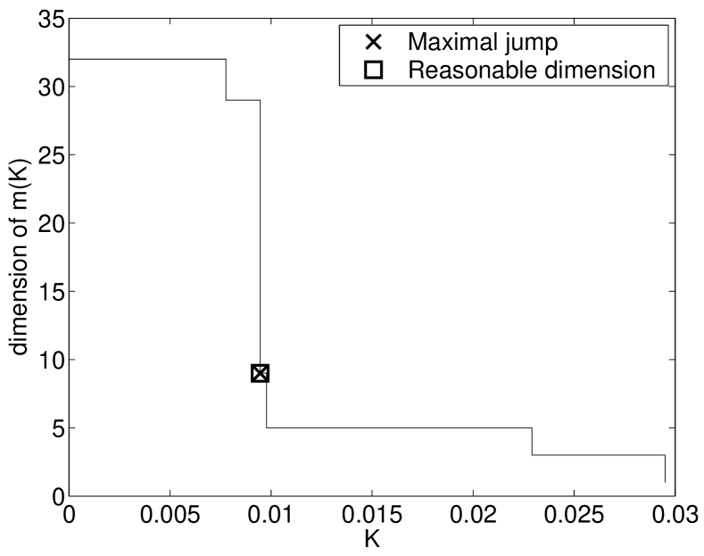
(a) One clear jump.

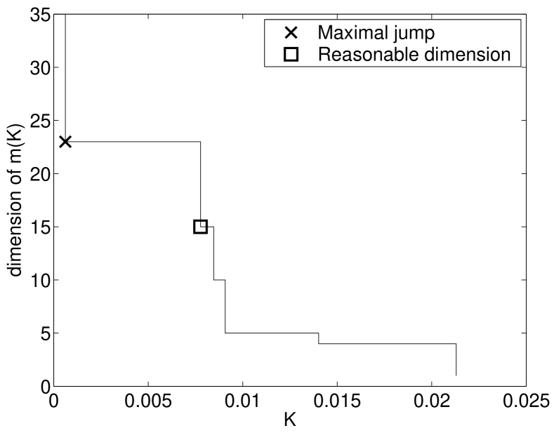
(b) Two jumps, two values for $\widehat{K}_{\min}$.

Figure 1: $D_{\widehat{m}(K)}$ as a function of $K$ for two different samples. Data are simulated according to (1) with $n=200$, $X_{i}\sim\mathcal{U}([0,1])$, $\epsilon_{i}\sim\mathcal{N}(0,1)$, $s(x)=\sin(\pi x)$ and $\sigma\equiv 1$. The models $(S_{m})_{m\in\mathcal{M}_{n}}$ are the sets of piecewise constant functions on regular partitions of $[0,1]$, with dimensions between 1 and $n/(\ln(n))$. The penalty shape is $\operatorname{pen}_{\mathrm{shape}}(m)=D_{m}$ and the dimension threshold is $D_{\mathrm{thresh}}=19\approx n/(2\ln(n))$. See experiment S1 by Arlot (2008c, Section 6.1) for details.

As an illustration, we compared the two definitions above (“threshold” and “maximal jump”) on $1\,000$ simulated samples. The exact simulation framework is described below Figure 1. Three cases occured:

1. There is one clear jump. Both definitions give the same value for $\widehat{K}_{\min}$. This occured for about $85\%$ of the samples; an example is given on Figure 1a.

2. There are several jumps corresponding to close values of $K$. Definitions (thresh) and (max jump) give slightly different values for $\widehat{K}_{\min}$, but the selected models $\widehat{m}\left(\left.2\widehat{K}_{\min}\right.\right)$ are equal. This occured for about $8.5\%$ of the samples.

3. There are several jumps corresponding to distant values of $K$. Definitions (thresh) and (max jump) strongly disagree, giving different selected models $\widehat{m}\left(\left.2\widehat{K}_{\min}\right.\right)$ at final. This occured for about $6.5\%$ of the samples; an example is given on Figure 1b.

The only problematic case is the third one, in which an arbitrary choice has to be made between definitions (thresh) and (max jump).

With the same simulated data, we have compared the prediction errors of the two methods by estimating the constant $C_{\mathrm{or}}$ that would appear in some oracle inequality,

$$C_{\mathrm{or}}:=\frac{\mathbb{E}\left[\left.\ell\left(\left.s,\widehat{s}_{\widehat{m}}\right.\right)\right.\right]}{\mathbb{E}\left[\left.\inf_{m\in\mathcal{M}_{n}}\left\{\left.\ell\left(\left.s,\widehat{s}_{m}\right.\right)\right.\right\}\right.\right]}\enspace.$$

With definition (thresh) $C_{\mathrm{or}}\approx 1.88$; with definition (max jump) $C_{\mathrm{or}}\approx 2.01$. For both methods, the standard error of the estimation is $0.04$. As a comparison, Mallows’ $C_{p}$ with a classical estimator of the variance $\sigma^{2}$ has an estimated performance $C_{\mathrm{or}}\approx 1.93$ on the same data.

The overall conclusion of this simulation experiment is that Algorithm 1 can be competitive with Mallows’ $C_{p}$ in a framework where Mallows’ $C_{p}$ is known to be optimal. Definition (thresh) for $\widehat{K}_{\min}$ seems slightly more efficient than (max jump), but without convincing evidence. Indeed, both definitions depend on some arbitrary choices: the value of the threshold $D_{\mathrm{thresh}}$ in (thresh), the maximal complexity among the collection of models $(S_{m})_{m\in\mathcal{M}_{n}}$ in (max jump). When $n$ is small, say $n=200$, choosing $D_{\mathrm{thresh}}$ is tricky since $n/(2\ln(n))$ and $\sqrt{n}$ are quite close. Then, the difference between (thresh) and (max jump) is likely to come mainly from the particular choice $D_{\mathrm{thresh}}=19$ than from basic differences between the two definitions.

In order to estimate $\widehat{K}_{\min}$ as automatically as possible, we suggest to combine the two definitions; when the selected models $\widehat{m}(2\widehat{K}_{\min})$ differ, send a warning to the final user advising him to look at the curve $K\mapsto D_{\widehat{m}(K)}$ himself; otherwise, remain confident in the automatic choice of $\widehat{m}(2\widehat{K}_{\min})$.

3.4 Penalty shape

For using Algorithm 1 in practice, it is necessary to know a priori, or at least to estimate, the optimal shape $\operatorname{pen}_{\mathrm{shape}}$ of the penalty. Let us explain how this can be achieved in different frameworks.

The first example that comes to mind is $\operatorname{pen}_{\mathrm{shape}}(m)=D_{m}$. It is valid for homoscedastic least-squares regression on linear models, as shown by several papers mentioned in Section 1. Indeed, when $\operatorname{Card}(\mathcal{M}_{n})$ is smaller than some power of $n$, Mallows’ $C_{p}$ penalty—defined by $\operatorname{pen}(m)=2\mathbb{E}\left[\left.\sigma^{2}(X)\right.\right]n^{-1}D_{m}$ —is well known to be asymptotically optimal. For larger collections $\mathcal{M}_{n}$, more elaborate results (Birgé and Massart, 2001, 2007) have shown that a penalty proportional to $\ln(n)\mathbb{E}\left[\left.\sigma^{2}(X)\right.\right]n^{-1}D_{m}$ and depending on the size of $\mathcal{M}_{n}$ is asymptotically optimal.

Algorithm 1 then provides an alternative to plugging an estimator of $\mathbb{E}\left[\left.\sigma^{2}(X)\right.\right]$ into the above penalties. Let us detail two main advantages of our approach. First, we avoid the difficult task of estimating $\mathbb{E}\left[\left.\sigma^{2}(X)\right.\right]$ without knowing in advance some model to which the true regression function belongs. Algorithm 1 provides a model-free estimation of the factor multiplying the penalty. Second, the estimator $\widehat{\sigma^{2}}$ of $\mathbb{E}\left[\left.\sigma^{2}(X)\right.\right]$ with the smallest quadratic risk is certainly far from being the optimal one for model selection. For instance, underestimating the multiplicative factor is well-known to lead to poor performances, whereas overestimating the multiplicative factor does not increase much the prediction error in general. Then, a good estimator of $\mathbb{E}\left[\left.\sigma^{2}(X)\right.\right]$ for model selection should overestimate it with a probability larger than $1/2$. Algorithm 1 satisfies this property automatically because $\widehat{K}_{\min}$ so that the selected model cannot be too large.

In short, Algorithm 1 with $\operatorname{pen}_{\mathrm{shape}}(m)=D_{m}$ is quite different from a simple plug-in version of Mallows’ $C_{p}$. It leads to a really data-dependent penalty, which may perform better in practice than the best deterministic penalty $K^{\star}D_{m}$.

In a more general framework, Algorithm 1 allows to choose a different shape of penalty $\operatorname{pen}_{\mathrm{shape}}$. For instance, in the heteroscedastic least-squares regression framework of Section 2.1, the optimal penalty is no longer proportional to the dimension $D_{m}$ of the models. This can be shown from computations made by (Arlot, 2008c, Proposition 1) when $S_{m}$ is assumed to be the vector space of piecewise constant functions on a partition $\left(\left.I_{\lambda}\right.\right)_{\lambda\in\Lambda_{m}}$ of $\mathcal{X}$:

$$\mathbb{E}\left[\left.\operatorname{pen}_{\mathrm{id}}(m)\right.\right]=\mathbb{E}\left[\left.(P-P_{n})\gamma\left(\left.\widehat{s}_{m}\right.\right)\right.\right]\approx\frac{2}{n}\sum_{\lambda\in\Lambda_{m}}\mathbb{E}\left[\left.\sigma(X)^{2}\,\right|\left.\,X\in I_{\lambda}\right.\right]\enspace.$$ (5)

An exact result has been proved by Arlot (2008c, Proposition 1). Moreover, Arlot (2008a) gave an example of model selection problem in which no penalty proportional to $D_{m}$ can be asymptotically optimal.

A first way to estimate the shape of the penalty is simply to use (5) to compute $\operatorname{pen}_{\mathrm{shape}}$, when both the distribution of $X$ and the shape of the noise level $\sigma$ are known. In practice, one has seldom such a prior knowledge.

We suggest in this situation to use resampling penalties (Efron, 1983; Arlot, 2008c), or $V$-fold penalties (Arlot, 2008b) which have much smaller computational costs. Up to a multiplicative factor (automatically estimated by Algorithm 1), these penalties should estimate correctly $\mathbb{E}\left[\left.\operatorname{pen}_{\mathrm{id}}(m)\right.\right]$ in any framework. In particular, resampling and $V$-fold penalties are asymptotically optimal in the heteroscedastic least-squares regression framework (Arlot, 2008b, c).

3.5 The general prediction framework

Section 2 and definition of Algorithm 1 have restricted ourselves to the least-squares regression framework. Actually, this is not necessary at all to make Algorithm 1 well-defined, so that it can naturally be extended to the general prediction framework. More precisely, the $(X_{i},Y_{i})$ can be assumed to belong to $\mathcal{X}\times\mathcal{Y}$ for some general $\mathcal{Y}$, and $\gamma:S\times(\mathcal{X}\times\mathcal{Y})\mapsto[0;+\infty)$ any contrast function. In particular, $\mathcal{Y}=\left\{\left.0,1\right.\right\}$ leads to the binary classification problem, for which a natural contrast function is the $0$–$1$ loss $\gamma(t;(x,y))=\mathds{1}_{t(x)\neq y}$. In this case, the shape of the penalty $\operatorname{pen}_{\mathrm{shape}}$ can for instance be estimated with the global or local Rademacher complexities mentioned in Section 1.

However, a natural question is whether the slope heuristics of Section 2.3, upon which Algorithm 1 relies, can be extended to the general framework. Several concentration results used to prove the validity of the slope heuristics in the least-squares regression framework in this article are valid in a general setting including binary classification. Even if the factor 2 coming from the closeness of $\mathbb{E}\left[\left.p_{1}\right.\right]$ and $\mathbb{E}\left[\left.p_{2}\right.\right]$ (see Section 2.3) may not be universally valid, we conjecture that Algorithm 1 can be used in other settings than least-squares regression. Moreover, as already mentioned at the end of Section 1, empirical studies have shown that Algorithm 1 can be successfully applied to several problems, with different shapes for the penalty. To our knowledge, to give a formal proof of this fact remains an interesting open problem.

4 Theoretical results

Algorithm 1 mainly relies on the “slope heuristics”, developed in Section 2.2. The goal of this section is to provide a theoretical justification of this heuristics.

It is split into two main results. First, Theorem 2 provides lower bounds on $D_{\widehat{m}}$ and the risk of $\widehat{s}_{\widehat{m}}$ when the penalty is smaller than $\operatorname{pen}_{\min}(m):=\mathbb{E}\left[\left.p_{2}(m)\right.\right]$. Second, Theorem 3 is an oracle inequality with leading constant almost one when $\operatorname{pen}(m)\approx 2\mathbb{E}\left[\left.p_{2}(m)\right.\right]$, relying on (3) and the comparison $p_{1}\approx p_{2}$.

In order to prove both theorems, two probabilistic results are necessary. First, $p_{1}$, $p_{2}$ and $\delta$ concentrate around their expectations; for $p_{2}$ and $\delta$, it is proved in a general framework in Appendix A.6. Second, $\mathbb{E}\left[\left.p_{1}(m)\right.\right]\approx\mathbb{E}\left[\left.p_{2}(m)\right.\right]$ for every $m\in\mathcal{M}_{n}$. The latter point is quite hard to prove in general, so that we must make an assumption on the models. Therefore, in this section, we restrict ourselves to the regressogram case, assuming that for every $m\in\mathcal{M}_{n}$, $S_{m}$ is the set of piecewise constant functions on some fixed partition $\left(\left.I_{\lambda}\right.\right)_{\lambda\in\Lambda_{m}}$ of $\mathcal{X}$. This framework is described precisely in the next subsection. Although we do not consider regressograms as a final goal, the theoretical results proved for regressograms help to understand better how to use Algorithm 1 in practice.

4.1 Regressograms

Let $S_{m}$ be the the set of piecewise constant functions on some partition $(I_{\lambda})_{\lambda\in\Lambda_{m}}$ of $\mathcal{X}$. The empirical risk minimizer $\widehat{s}_{m}$ on $S_{m}$ is called a regressogram. $S_{m}$ is a vector space of dimension $D_{m}=\operatorname{Card}(\Lambda_{m})$, spanned by the family $(\mathds{1}_{I_{\lambda}})_{\lambda\in\Lambda_{m}}$. Since this basis is orthogonal in $L^{2}(\mu)$ for any probability measure $\mu$ on $\mathcal{X}$, computations are quite easy. In particular, we have:

$$s_{m}=\sum_{\lambda\in\Lambda_{m}}\beta_{\lambda}\mathds{1}_{I_{\lambda}}\quad\mbox{and}\quad\widehat{s}_{m}=\sum_{\lambda\in\Lambda_{m}}\widehat{\beta}_{\lambda}\mathds{1}_{I_{\lambda}}\enspace,$$

where

$$\beta_{\lambda}:=\mathbb{E}_{P}\left[\left.Y\,\right|\left.\,X\in I_{\lambda}\right.\right]\qquad\widehat{\beta}_{\lambda}:=\frac{1}{n\widehat{p}_{\lambda}}\sum_{X_{i}\in I_{\lambda}}Y_{i}\qquad\widehat{p}_{\lambda}:=P_{n}(X\in I_{\lambda})\enspace.$$

Note that $\widehat{s}_{m}$ is uniquely defined if and only if each $I_{\lambda}$ contains at least one of the $X_{i}$. Otherwise, $\widehat{s}_{m}$ is not uniquely defined and we consider that the model $m$ cannot be chosen.

4.2 Main assumptions

In this section, we make the following assumptions. First, each model $S_{m}$ is a set of piecewise constants functions on some fixed partition $(I_{\lambda})_{\lambda\in\Lambda_{m}}$ of $X$. Second, the family $(S_{m})_{m\in\mathcal{M}_{n}}$ satisfies:

1. Polynomial complexity of $\mathcal{M}_{n}$: $\operatorname{Card}(\mathcal{M}_{n})\leq c_{\mathcal{M}}n^{\alpha_{\mathcal{M}}}$.

2. Richness of $\mathcal{M}_{n}$: $\exists m_{0}\in\mathcal{M}_{n}$ s.t. $D_{m_{0}}\in\left[\left.\sqrt{n},c_{\mathrm{rich}}\sqrt{n}\right.\right]$.

Assumption $\mathbf{(P1)}$ is quite classical for proving the asymptotic optimality of a model selection procedure; it is for instance implicitly assumed by Li (1987) in the homoscedastic fixed-design case. Assumption $\mathbf{(P2)}$ is merely technical and can be changed if necessary; it only ensures that $(S_{m})_{m\in\mathcal{M}_{n}}$ does not contain only models which are either too small or too large.

For any penalty function $\operatorname{pen}:\mathcal{M}_{n}\mapsto\mathbb{R}^{+}$, we define the following model selection procedure:

$$\widehat{m}\in\arg\min_{m\in\mathcal{M}_{n},\,\min_{\lambda\in\Lambda_{m}}\left\{\left.\widehat{p}_{\lambda}\right.\right\}>0}\left\{\left.P_{n}\gamma(\widehat{s}_{m})+\operatorname{pen}(m)\right.\right\}\enspace.$$ (6)

Moreover, the data $(X_{i},Y_{i})_{1\leq i\leq n}$ are assumed to be i.i.d. and to satisfy:

1. The data are bounded: $\left\lVert Y_{i}\right\rVert_{\infty}\leq A<\infty$.

2. Uniform lower-bound on the noise level: $\sigma(X_{i})\geq\sigma_{\min}>0$ a.s.

3. The bias decreases as a power of $D_{m}$: there exist some $\beta_{+},C_{+}>0$ such that

   $$\ell\left(\left.s,s_{m}\right.\right)\leq C_{+}D_{m}^{-\beta_{+}}\enspace.$$

4. Lower regularity of the partitions for $\mathcal{L}(X)$: $D_{m}\min_{\lambda\in\Lambda_{m}}\left\{\left.\mathbb{P}\left(\left.X\in I_{\lambda}\right.\right)\right.\right\}\geq c_{\mathrm{r},\ell}^{X}$.

Further comments are made in Sections 4.3 and 4.4 about these assumptions, in particular about their possible weakening.

4.3 Minimal penalties

Our first result concerns the existence of a minimal penalty. In this subsection, $\mathbf{(P2)}$ is replaced by the following strongest assumption:

1. $\exists c_{0},c_{\mathrm{rich}}>0$ s.t. $\forall l\in\left[\left.\sqrt{n},c_{0}n/(c_{\mathrm{rich}}\ln(n))\right.\right]$, $\exists m\in\mathcal{M}_{n}$ s.t. $D_{m}\in\left[\left.l,c_{\mathrm{rich}}l\right.\right]$.

The reason why $\mathbf{(P2)}$ is not sufficient to prove Theorem 2 below is that at least one model of dimension of order $n/\ln(n)$ should belong to the family $\left(\left.S_{m}\right.\right)_{m\in\mathcal{M}_{n}}$; otherwise, it may not be possible to prove that such models are selected by penalization procedures beyond the minimal penalty.

Theorem 2

Suppose all the assumptions of Section 4.2 are satisfied. Let $K\in[0;1)$, $L>0$, and assume that an event of probability at least $1-Ln^{-2}$ exists on which

$$\forall m\in\mathcal{M}_{n},\quad 0\leq\operatorname{pen}(m)\leq K\mathbb{E}\left[\left.P_{n}\left(\left.\gamma(s_{m})-\gamma(\widehat{s}_{m})\right.\right)\right.\right]\enspace.$$ (7)

Then, there exist two positive constants $K_{1}$, $K_{2}$ such that, with probability at least $1-K_{1}n^{-2}$,

$$D_{\widehat{m}}\geq K_{2}n\ln(n)^{-1}\enspace,$$

where $\widehat{m}$ is defined by (6). On the same event,

$$\ell\left(\left.s,\widehat{s}_{\widehat{m}}\right.\right)\geq\ln(n)\inf_{m\in\mathcal{M}_{n}}\left\{\left.\ell\left(\left.s,\widehat{s}_{m}\right.\right)\right.\right\}\enspace.$$ (8)

The constants $K_{1}$ and $K_{2}$ may depend on $K$, $L$ and constants in $\mathbf{(P1)}$, $\mathbf{(P2+)}$, $\mathbf{(Ab)}$, $\mathbf{(An)}$, $\mathbf{(Ap_{u})}$ and $\mathbf{(Ar^{X}_{\ell})}$, but do not depend on $n$.

This theorem thus validates the first part of the heuristics of Section 2.3, proving that a minimal amount of penalization is required; when the penalty is smaller, the selected dimension $D_{\widehat{m}}$ and the quadratic risk of the final estimator $\ell\left(\left.s,\widehat{s}_{\widehat{m}}\right.\right)$ blow up. This coupling is quite interesting, since the dimension $D_{\widehat{m}}$ is known in practice, contrary to $\ell\left(\left.s,\widehat{s}_{\widehat{m}}\right.\right)$. It is then possible to detect from the data whether the penalty is too small, as proposed in Algorithm 1.

The main interest of this result is its combination with Theorem 3 below. Nevertheless Theorem 2 is also interesting by itself for understanding the theoretical properties of penalization procedures. Indeed, it generalizes the results of Birgé and Massart (2007) on the existence of minimal penalties to heteroscedastic regression with a random design, even if we have to restrict to regressograms. Moreover, we have a general formulation for the minimal penalty

$$\operatorname{pen}_{\min}(m):=\mathbb{E}\left[\left.P_{n}\left(\left.\gamma(s_{m})-\gamma(\widehat{s}_{m})\right.\right)\right.\right]=\mathbb{E}\left[\left.p_{2}(m)\right.\right]\enspace,$$

which can be used in frameworks situations where it is not proportional to the dimension $D_{m}$ of the models (see Section 3.4 and references therein).

In addition, assumptions $\mathbf{(Ab)}$ and $\mathbf{(An)}$ on the data are much weaker than the Gaussian homoscedastic assumption. They are also much more realistic, and moreover can be strongly relaxed. Roughly speaking, boundedness of data can be replaced by conditions on moments of the noise, and the uniform lower bound $\sigma_{\min}$ is no longer necessary when $\sigma$ satisfies some mild regularity assumptions. We refer to Arlot (2008c, Section 4.3) for detailed statements of these assumptions, and explanations on how to adapt proofs to these situations.

Finally, let us comment on conditions $\mathbf{(Ap_{u})}$ and $\mathbf{(Ar^{X}_{\ell})}$. The upper bound $\mathbf{(Ap_{u})}$ on the bias occurs in the most reasonable situations, for instance when $\mathcal{X}\subset\mathbb{R}^{k}$ is bounded, the partition $\left(\left.I_{\lambda}\right.\right)_{\lambda\in\Lambda_{m}}$ is regular and the regression function $s$ is $\alpha$-Hölderian for some $\alpha>0$ ($\beta_{+}$ depending on $\alpha$ and $k$). It ensures that medium and large models have a significantly smaller bias than smaller ones; otherwise, the selected dimension would be allowed to be too small with significant probability. On the other hand, $\mathbf{(Ar^{X}_{\ell})}$ is satisfied at least for “almost regular” partitions $\left(\left.I_{\lambda}\right.\right)_{\lambda\in\Lambda_{m}}$, when $X$ has a lower bounded density w.r.t. the Lebesgue measure on $\mathcal{X}\subset\mathbb{R}^{k}$.

Theorem 2 is stated with a general formulation of $\mathbf{(Ap_{u})}$ and $\mathbf{(Ar^{X}_{\ell})}$, instead of assuming for instance that $s$ is $\alpha$-Hölderian and $X$ has a lower bounded density w.r.t $\operatorname{Leb}$, in order to point out the generality of the “minimal penalization” phenomenon. It occurs as soon as the models are not too much pathological. In particular, we do not make any assumption on the distribution of $X$ itself, but only that the models are not too badly chosen according to this distribution. Such a condition can be checked in practice if some prior knowledge on $\mathcal{L}(X)$ is available; if part of the data are unlabeled—a usual case—, classical density estimation procedures can be applied for estimating $\mathcal{L}(X)$ from unlabeled data (Devroye and Lugosi, 2001).

4.4 Optimal penalties

Algorithm 1 relies on a link between the minimal penalty pointed out by Theorem 2 and some optimal penalty. The following result is a formal proof of this link in the framework we consider: penalties close to twice the minimal penalty satisfy an oracle inequality with leading constant approximately equal to one.

Theorem 3

Suppose all the assumptions of Section 4.2 are satisfied together with

1. The bias decreases like a power of $D_{m}$: there exist $\beta_{-}\geq\beta_{+}>0$ and $C_{+},C_{-}>0$ such that

   $$C_{-}D_{m}^{-\beta_{-}}\leq\ell\left(\left.s,s_{m}\right.\right)\leq C_{+}D_{m}^{-\beta_{+}}\enspace.$$

Let $\delta\in(0,1)$, $L>0$, and assume that an event of probability at least $1-Ln^{-2}$ exists on which for every $m\in\mathcal{M}_{n}$,

$$(2-\delta)\mathbb{E}\left[\left.P_{n}\left(\left.\gamma(s_{m})-\gamma(\widehat{s}_{m})\right.\right)\right.\right]\leq\operatorname{pen}(m)\leq(2+\delta)\mathbb{E}\left[\left.P_{n}\left(\left.\gamma(s_{m})-\gamma(\widehat{s}_{m})\right.\right)\right.\right]\enspace.$$ (9)

Then, for every $0<\eta<\min\left\{\left.\beta_{+};1\right.\right\}/2$, there exist a constant $K_{3}$ and a sequence $\epsilon_{n}$ tending to zero at infinity such that, with probability at least $1-K_{3}n^{-2}$,

$$D_{\widehat{m}} \leq n^{1-\eta}$$

$$\mbox{and}\qquad\ell\left(\left.s,\widehat{s}_{\widehat{m}}\right.\right) \leq\left(\left.\frac{1+\delta}{1-\delta}+\epsilon_{n}\right.\right)\inf_{m\in\mathcal{M}_{n}}\left\{\left.\ell\left(\left.s,\widehat{s}_{m}\right.\right)\right.\right\}\enspace,$$ (10)

where $\widehat{m}$ is defined by (6). Moreover, we have the oracle inequality

$$\mathbb{E}\left[\left.\ell\left(\left.s,\widehat{s}_{\widehat{m}}\right.\right)\right.\right]\leq\left(\left.\frac{1+\delta}{1-\delta}+\epsilon_{n}\right.\right)\mathbb{E}\left[\left.\inf_{m\in\mathcal{M}_{n}}\left\{\left.\ell\left(\left.s,\widehat{s}_{m}\right.\right)\right.\right\}\right.\right]+\frac{A^{2}K_{3}}{n^{2}}\enspace.$$

The constant $K_{3}$ may depend on $L,\delta,\eta$ and the constants in $\mathbf{(P1)}$, $\mathbf{(P2)}$, $\mathbf{(Ab)}$, $\mathbf{(An)}$, $\mathbf{(Ap)}$ and $\mathbf{(Ar^{X}_{\ell})}$, but not on $n$. The term $\epsilon_{n}$ is smaller than $\ln(n)^{-1/5}$; it can be made smaller than $n^{-\delta}$ for any $\delta\in(0;\delta_{0}(\beta_{-},\beta_{+}))$ at the price of enlarging $K_{3}$.

This theorem shows that twice the minimal penalty $\operatorname{pen}_{\min}$ pointed out by Theorem 2 satisfies an oracle inequality with leading constant almost one. In other words, the slope heuristics of Section 2.3 is valid. The consequences of the combination of Theorems 2 and 3 are detailed in Section 4.5.

The oracle inequality (10) remains valid when the penalty is only close to twice the minimal one. In particular, the shape of the penalty can be estimated by resampling as suggested in Section 3.4.

Actually, Theorem 3 above is a corollary of a more general result stated in Appendix A.3, Theorem 5. If

$$\operatorname{pen}(m)\approx K\mathbb{E}\left[\left.P_{n}\left(\left.\gamma(s_{m})-\gamma(\widehat{s}_{m})\right.\right)\right.\right]$$ (11)

instead of (9), under the same assumptions, an oracle inequality with leading constant $C(K)+\epsilon_{n}$ instead of $1+\epsilon_{n}$ holds with large probability. The constant $C(K)$ is equal to $(K-1)^{-1}$ when $K\in(1,2]$ and to $C(K)=K-1$ when $K>2$. Therefore, for every $K>1$, the penalty defined by (11) is efficient up to a multiplicative constant. This result is new in the heteroscedastic framework.

Let us comment the additional assumption $\mathbf{(Ap)}$, that is the lower bound on the bias. Assuming $\ell\left(\left.s,s_{m}\right.\right)>0$ for every $m\in\mathcal{M}_{n}$ is classical for proving the asymptotic optimality of Mallows’ $C_{p}$ (Shibata, 1981; Li, 1987; Birgé and Massart, 2007). $\mathbf{(Ap)}$ has been made by Stone (1985) and Burman (2002) in the density estimation framework, for the same technical reasons as ours. Assumption $\mathbf{(Ap)}$ is satisfied in several frameworks, such as the following: $(I_{\lambda})_{\lambda\in\Lambda_{m}}$ is “regular”, $X$ has a lower-bounded density w.r.t. the Lebesgue measure on $\mathcal{X}\subset\mathbb{R}^{k}$, and $s$ is non-constant and $\alpha$-hölderian (w.r.t. $\left\lVert\cdot\right\rVert_{\infty}$), with

$$\beta_{1}=k^{-1}+\alpha^{-1}-(k-1)k^{-1}\alpha^{-1}\qquad\mbox{and}\qquad\beta_{2}=2\alpha k^{-1}\enspace.$$

We refer to Arlot (2007, Section 8.10) for a complete proof.

When the lower bound in $\mathbf{(Ap)}$ is no longer assumed, (10) holds with two modifications in its right-hand side (for details, see Arlot, 2008c, Remark 9): the $\inf$ is restricted to models of dimension larger than $\ln(n)^{\gamma_{1}}$, and there is a remainder term $\ln(n)^{\gamma_{2}}n^{-1}$, where $\gamma_{1},\gamma_{2}>0$ are numerical constants. This is equivalent to (10), unless there is a model of small dimension with a small bias. The lower bound in $\mathbf{(Ap)}$ ensures that it cannot happen. Note that if there is a small model close to $s$, it is hopeless to obtain an oracle inequality with a penalty which estimates $\operatorname{pen}_{\mathrm{id}}$, simply because deviations of $\operatorname{pen}_{\mathrm{id}}$ around its expectation would be much larger than the excess loss of the oracle. In such a situation, BIC-like methods are more appropriate; for instance, Csiszár (2002) and Csiszár and Shields (2000) showed that BIC penalties are minimal penalties for estimating the order of a Markov chain.

4.5 Main theoretical and practical consequences

The slope heuristics and the correctness of Algorithm 1 follow from the combination of Theorems 2 and 3.

4.5.1 Optimal and minimal penalties

For the sake of simplicity, let us consider the penalty $K\mathbb{E}\left[\left.p_{2}(m)\right.\right]$ with any $K>0$; any penalty close to this one satisfies similar properties. At first reading, one can think of the homoscedastic case where $\mathbb{E}\left[\left.p_{2}(m)\right.\right]\approx\sigma^{2}D_{m}n^{-1}$; one of the novelties of our results is that the general picture is quite similar.

According to Theorem 3, the penalization procedure associated with $K\mathbb{E}\left[\left.p_{2}(m)\right.\right]$ satisfies an oracle inequality with leading constant $C_{n}(K)$ as soon as $K>1$, and $C_{n}(2)\approx 1$. Moreover, results proved by Arlot (2008b) imply that $C_{n}(K)\geq C(K)>1$ as soon as $K$ is not close to 2. Therefore, $K=2$ is the optimal multiplying factor in front of $\mathbb{E}\left[\left.p_{2}(m)\right.\right]$.

When $K<1$, Theorem 2 shows that no oracle inequality can hold with leading constant $C_{n}(K)<\ln(n)$. Since $C_{n}(K)\leq(K-1)^{-1}<\ln(n)$ as soon as $K>1+\ln(n)^{-1}$, $K=1$ is the minimal multiplying factor in front of $\mathbb{E}\left[\left.p_{2}(m)\right.\right]$. More generally, $\operatorname{pen}_{\min}(m):=\mathbb{E}\left[\left.p_{2}(m)\right.\right]$ is proved to be a minimal penalty.

In short, Theorems 2 and 3 prove the slope heuristics described in Section 2.3:

$$\mbox{\em``optimal'' penalty}\approx 2\times\mbox{\em``minimal'' penalty}\enspace.$$

Birgé and Massart (2007) have proved the validity of the slope heuristics in the Gaussian homoscedastic framework. This paper extends their result to a non-Gaussian and heteroscedastic setting.

4.5.2 Dimension jump

In addition, Theorems 2 and 3 prove the existence of a crucial phenomenon: there exists a “dimension jump”—complexity jump in the general framework—around the minimal penalty. Let us consider again the penalty $K\mathbb{E}\left[\left.p_{2}(m)\right.\right]$. As in Algorithm 1, let us define

$$\widehat{m}(K)\in\arg\min_{m\in\mathcal{M}_{n}}\left\{\left.P_{n}\gamma\left(\left.\widehat{s}_{m}\right.\right)+K\mathbb{E}\left[\left.p_{2}(m)\right.\right]\right.\right\}\enspace.$$

A careful look at the proofs of Theorems 2 and 3 shows that there exist constants $K_{4},K_{5}>0$ and an event of probability $1-K_{4}n^{-2}$ on which

$$\forall 0<K<1-\frac{1}{\ln(n)},\,D_{\widehat{m}(K)}\geq\frac{K_{5}n}{(\ln(n))^{2}}\,\,\mbox{ and }\,\,\forall K>1+\frac{1}{\ln(n)},\,D_{\widehat{m}(K)}\leq n^{1-\eta}\enspace.$$ (12)

Therefore, the dimension $D_{\widehat{m}(K)}$ of the selected model jumps around the minimal value $K=1$, from values of order $n(\ln(n))^{-2}$ to $n^{1-\eta}$.

Let us know explain why Algorithm 1 is correct, assuming that $\operatorname{pen}_{\mathrm{shape}}(m)$ is close to $\mathbb{E}\left[\left.p_{2}(m)\right.\right]$. With definition (thresh) of $\widehat{K}_{\min}$ and a threshold $D_{\mathrm{thresh}}\propto n(\ln(n))^{-3}$, (12) ensures that

$$1-\frac{1}{\ln(n)}\leq\widehat{K}_{\min}\leq 1+\frac{1}{\ln(n)}$$

with a large probability. Then, according to Theorem 3, the output of Algorithm 1 satisfies an oracle inequality with leading constant $C_{n}$ tending to one as $n$ tends to infinity.

4.6 Comparison with data-splitting methods

Tuning parameters are often chosen by cross-validation or by another data-splitting method, which suffer from some drawbacks compared to Algorithm 1.

First, $V$-fold cross-validation, leave-$p$-out and repeated learning-testing methods require a larger computation time. Indeed, they need to perform the empirical risk minimization process for each model several times, whereas Algorithm 1 only needs to perform it once.

Second, $V$-fold cross-validation is asymptotically suboptimal when $V$ is fixed, as shown by (Arlot, 2008b, Theorem 1). The same suboptimality result is valid for the hold-out, when the size of the training set is not asymptotically equivalent to the sample size $n$. On the contrary, Theorems 2 and 3 prove that Algorithm 1 is asymptotically optimal in a framework including the one used by (Arlot, 2008b, Theorem 1) for proving the suboptimality of $V$-fold cross-validation. Hence, the quadratic risk of Algorithm 1 should be smaller, within a factor $\kappa>1$.

Third, hold-out with a training set of size $n_{t}\sim n$, for instance $n_{t}=n-\sqrt{n}$ or $n_{t}=n(1-\ln(n)^{-1})$, is known to be unstable. The final output $\widehat{m}$ strongly depends on the choice of a particular split of the data. According to the simulation study of Section 3.3, Algorithm 1 is far more stable.

To conclude, compared to data splitting methods, Algorithm 1 is either faster to compute, more efficient in terms of quadratic risk, or more stable. Then, Algorithm 1 should be preferred each time it can be used. Another approach is to use aggregation techniques, instead of selecting one model. As shown by several results (see for instance Tsybakov, 2004; Lecué, 2007), aggregating estimators built upon a training simple of size $n_{t}\sim n$ can have an optimal quadratic risk. Moreover, aggregation requires approximately the same computation time as Algorithm 1, and is much more stable than the hold-out. Hence, it can be an alternative to model selection with Algorithm 1.

5 Conclusion

This paper provides mathematical evidence that the method introduced by Birgé and Massart (2007) for designing data-driven penalties remains efficient in a non-Gaussian framework. The purpose of this conclusion is to relate the slope heuristics developed in Section 2 to the well known Mallows’ $C_{p}$ and Akaike’s criteria and to the unbiased estimation of the risk principle.

Let us come come back to Gaussian model selection in order to explain how to guess what is the right penalty from the data themselves. Let $\gamma_{n}$ be some empirical criterion (for instance the least-squares criterion as in this paper, or the log-likelihood criterion), $\left(\left.S_{m}\right.\right)_{m\in\mathcal{M}_{n}}$ be a collection of models and for every $m\in\mathcal{M}_{n}$ $s_{m}$ be some minimizer of $t\mapsto\mathbb{E}\left[\left.\gamma_{n}\left(\left.t\right.\right)\right.\right]$ over $S_{m}$ (assuming that such a point exists). Minimizing some penalized criterion

$$\gamma_{n}\left(\left.\widehat{s}_{m}\right.\right)+\operatorname{pen}(m)$$

over $\mathcal{M}_{n}$ amounts to minimize

$$\widehat{b}_{m}-\widehat{v}_{m}+\operatorname{pen}(m)\enspace,$$

$$\mbox{where}\quad\forall m\in\mathcal{M}_{n},\,\,\widehat{b}_{m}=\gamma_{n}\left(\left.s_{m}\right.\right)-\gamma_{n}\left(\left.s\right.\right)\mbox{ and }\widehat{v}_{m}=\gamma_{n}\left(\left.s_{m}\right.\right)-\gamma_{n}\left(\left.\widehat{s}_{m}\right.\right)\enspace.$$

The point is that $\widehat{b}_{m}$ is an unbiased estimator of the bias term $\ell\left(\left.s,s_{m}\right.\right)$. Having concentration arguments in mind, minimizing $\widehat{b}_{m}-\widehat{v}_{m}+\operatorname{pen}(m)$ can be conjectured approximately equivalent to minimize

$$\ell\left(\left.s,s_{m}\right.\right)-\mathbb{E}\left[\left.\widehat{v}_{m}\right.\right]+\operatorname{pen}(m)\enspace.$$

Since the purpose of model selection is to minimize the risk $\mathbb{E}\left[\left.\ell\left(\left.s,\widehat{s}_{m}\right.\right)\right.\right]$, an ideal penalty would be

$$\operatorname{pen}(m)=\mathbb{E}\left[\left.\widehat{v}_{m}\right.\right]+\mathbb{E}\left[\left.\ell\left(\left.s_{m},\widehat{s}_{m}\right.\right)\right.\right]\enspace.$$

In Gaussian least-squares regression with a fixed design, the models $S_{m}$ are linear and $\mathbb{E}\left[\left.\widehat{v}_{m}\right.\right]=\mathbb{E}\left[\left.\ell\left(\left.s_{m},\widehat{s}_{m}\right.\right)\right.\right]$ is explicitly computable if the noise level is constant and known; this leads to Mallows’ $C_{p}$ penalty. When $\gamma_{n}$ is the log-likelihood,

$$\mathbb{E}\left[\left.\widehat{v}_{m}\right.\right]\approx\mathbb{E}\left[\left.\ell\left(\left.s_{m},\widehat{s}_{m}\right.\right)\right.\right]\approx\frac{D_{m}}{2n}$$

asymptotically, where $D_{m}$ stands for the number of parameters defining model $S_{m}$; this leads to Akaike’s Information Criterion (AIC). Therefore, both Mallows’ $C_{p}$ and Akaike’s criterion are based on the unbiased (or asymptotically unbiased) risk estimation principle.

This paper goes further in this direction, using that $\mathbb{E}\left[\left.\widehat{v}_{m}\right.\right]\approx\mathbb{E}\left[\left.\ell\left(\left.s_{m},\widehat{s}_{m}\right.\right)\right.\right]$ remains a valid approximation in a non-asymptotic framework. Then, a good penalty becomes $2\mathbb{E}\left[\left.\widehat{v}_{m}\right.\right]$ or $2\widehat{v}_{m}$, having in mind concentration arguments. Since $\widehat{v}_{m}$ is the minimal penalty, this explains the slope heuristics (Birgé and Massart, 2007) and connects it to Mallows’ $C_{p}$ and Akaike’s heuristics.

The second main idea developed in this paper is that the minimal penalty can be estimated from the data; Algorithm 1 uses the jump of complexity which occurs around the minimal penalty, as shown in Sections 3.3 and 4.5.2. Another way to estimate the minimal penalty when it is (at least approximately) of the form $\alpha D_{m}$ is to estimate $\alpha$ by the slope of the graph of $\gamma_{n}\left(\left.\widehat{s}_{m}\right.\right)$ for large enough values of $D_{m}$; this method can be extended to other shapes of penalties, simply by replacing $D_{m}$ by some (known!) function $f\left(\left.D_{m}\right.\right)$.

The slope heuristics can even be combined with resampling ideas, by taking a function $f$ built from a randomized empirical criterion. As shown by Arlot (2008a), this approach is much more efficient than the rougher choice $f\left(\left.D_{m}\right.\right)=D_{m}$ for heteroscedastic regression frameworks. The question of the optimality of the slope heuristics in general remains an open problem; nevertheless, we believe that this heuristics can be useful in practice, and that proving its efficiency in this paper helps to understand it better.

Let us finally mention that contrary to Birgé and Massart (2007), we assume in this paper that the collection of models $\mathcal{M}_{n}$ is “small”, that is $\operatorname{Card}(\mathcal{M}_{n})$ grows at most like a power of $n$. For several problems, such that complete variable selection, larger collections of models have to be considered; then, it is known from the homoscedastic case that the minimal penalty is much larger than $\mathbb{E}\left[\left.p_{2}(m)\right.\right]$. Nevertheless, Émilie Lebarbier has used the slope heuristics with $f\left(\left.D_{m}\right.\right)=D_{m}\left(\left.2.5+\ln\left(\left.\frac{n}{D_{m}}\right.\right)\right.\right)$ for multiple change-points detection from $n$ noisy data, using the results by Birgé and Massart (2007) in the Gaussian case.

Let us now explain how we expect to generalize the slope heuristics to the non-Gaussian heteroscedastic case when $\mathcal{M}_{n}$ is large. First, group the models according to some complexity index $C_{m}$ such as their dimensions $D_{m}$; for $C\in\left\{\left.1,\ldots,n^{k}\right.\right\}$, define $\widetilde{S_{C}}=\bigcup_{C_{m}=C}S_{m}$. Then, replace the model selection problem with the family $(S_{m})_{m\in\mathcal{M}_{n}}$ by a “complexity selection problem”, that is model selection with the family $\left(\left.\widetilde{S_{C}}\right.\right)_{1\leq C\leq n^{k}}$. We conjecture that this grouping of the models is sufficient to take into account the richness of $\mathcal{M}_{n}$ for the optimal calibration of the penalty. A theoretical justification of this point could rely on the extension of our results to any kind of model, since $\widetilde{S_{C}}$ is not a vector space in general.

Acknowledgments

The authors gratefully acknowledge the anonymous referees for several suggestions and references.

A Proofs

This appendix is devoted to the proofs of the results stated in the paper. Proposition 1 is proved in Section A.2; Theorem 3 is proved in Sections A.3 and A.4; Theorem 2 is proved in Section A.5; the remaining sections are devoted to probabilistic results used in the main proofs and technical proofs.

A.1 Conventions and notations

In the rest of the paper, $L$ denotes a universal constant, not necessarily the same at each occurrence. When $L$ is not universal, but depends on $p_{1},\ldots,p_{k}$, it is written $L_{p_{1},\ldots,p_{k}}$. Similarly, $L_{\mathbf{(SH2)}}$ (resp. $L_{\mathbf{(SH5)}}$) denotes a constant allowed to depend on the parameters of the assumptions made in Theorem 2 (resp. Theorem 5), including $\mathbf{(P1)}$ and $\mathbf{(P2)}$. We also make use of the following notations:

• $\forall a,b\in\mathbb{R}$, $a\wedge b$ is the minimum of $a$ and $b$, $a\vee b$ is the maximum of $a$ and $b$, $a_{+}=a\vee 0$ is the positive part of $a$ and $a_{-}=a\wedge 0$ is its negative part.

• $\forall I_{\lambda}\subset\mathcal{X}$, $p_{\lambda}:=P(X\in I_{\lambda})$ and $\sigma_{\lambda}^{2}:=\mathbb{E}\left[\left.\left(\left.Y-s_{m}(X)\right.\right)^{2}\,\right|\left.\,X\in I_{\lambda}\right.\right]$.

• Since $\mathbb{E}\left[\left.p_{1}(m)\right.\right]$ is not well-defined (because of the event $\left\{\left.\min_{\lambda\in\Lambda_{m}}\left\{\left.\widehat{p}_{\lambda}\right.\right\}=0\right.\right\}$), we have to take the following convention

  $$p_{1}(m)=\widetilde{p_{1}}(m):=\sum_{\lambda\in\Lambda_{m}\,\mbox{ s.t. }\,\widehat{p}_{\lambda}>0}p_{\lambda}\left(\left.\beta_{\lambda}-\widehat{\beta}_{\lambda}\right.\right)^{2}+\sum_{\lambda\in\Lambda_{m}\,\mbox{ s.t. }\,\widehat{p}_{\lambda}=0}p_{\lambda}\sigma_{\lambda}^{2}\enspace.$$

  Remark that $p_{1}(m)=\widetilde{p_{1}}(m)$ when $\min_{\lambda\in\Lambda_{m}}\left\{\left.\widehat{p}_{\lambda}\right.\right\}>0$), so that this convention has no consequences on the final results (Theorems 2 and 5).

A.2 Proof of Proposition 1

First, since $\mathcal{M}_{n}$ is finite, the infimum in (4) is attained as soon as $G(m_{i-1})\neq\emptyset$, so that $m_{i}$ is well defined for every $i\leq i_{\max}$. Moreover, by construction, $g(m_{i})$ decreases with $i$, so that all the $m_{i}\in\mathcal{M}_{n}$ are different; hence, Algorithm 2 terminates and $i_{\max}+1\leq\operatorname{Card}(\mathcal{M}_{n})$. We now prove by induction the following property for every $i\in\left\{\left.0,\ldots,i_{\max}\right.\right\}$:

$$\mathcal{P}_{i}:\qquad K_{i}<K_{i+1}\quad\mbox{ and }\quad\forall K\in[K_{i},K_{i+1}),\quad\widehat{m}(K)=m_{i}\enspace.$$

Notice also that $K_{i}$ can always be defined by (4) with the convention $\inf\emptyset=+\infty$.

$\mathcal{P}_{0}$ holds true

By definition of $K_{1}$, it is clear that $K_{1}>0$ (it may be equal to $+\infty$ if $G(m_{0})=\emptyset$). For $K=K_{0}=0$, the definition of $m_{0}$ is the one of $\widehat{m}(0)$, so that $\widehat{m}(K)=m_{0}$. For $K\in(0,K_{1})$, Lemma 4 shows that either $\widehat{m}(K)=\widehat{m}(0)=m_{0}$ or $\widehat{m}(K)\in G(0)$. In the latter case, by definition of $K_{1}$,

$$\frac{f(\widehat{m}(K))-f(m_{0})}{g(m_{0})-g(\widehat{m}(K))}\geq K_{1}>K$$

hence

$$f(\widehat{m}(K))+Kg(\widehat{m}(K))>f(m_{0})+Kg(m_{0})$$

which is contradictory with the definition of $\widehat{m}(K)$. Therefore, $\mathcal{P}_{0}$ holds true.

$\mathcal{P}_{i}\Rightarrow\mathcal{P}_{i+1}$ for every $i\in\left\{\left.0,\ldots,i_{\max}-1\right.\right\}$

Assume that $\mathcal{P}_{i}$ holds true. First, we have to prove that $K_{i+2}>K_{i+1}$. Since $K_{i_{\max}+1}=+\infty$, this is clear if $i=i_{\max}-1$. Otherwise, $K_{i+2}<+\infty$ and $m_{i+2}$ exists. Then, by definition of $m_{i+2}$ and $K_{i+2}$ (resp. $m_{i+1}$ and $K_{i+1}$), we have

$$f(m_{i+2})-f(m_{i+1})=K_{i+2}(g(m_{i+1})-g(m_{i+2}))$$ (13)

$$f(m_{i+1})-f(m_{i})=K_{i+1}(g(m_{i})-g(m_{i+1}))\enspace.$$ (14)

Moreover, $m_{i+2}\in G(m_{i+1})\subset G(m_{i})$, and $m_{i+2}\prec m_{i+1}$ (because $g$ is non-decreasing). Using again the definition of $K_{i+1}$, we have

$$f(m_{i+2})-f(m_{i})>K_{i+1}(g(m_{i})-g(m_{i+2}))$$ (15)

(otherwise, we would have $m_{i+2}\in F_{i+1}$ and $m_{i+2}\prec m_{i+1}$, which is not possible). Combining the difference of (15) and (14) with (13), we have

$$K_{i+2}(g(m_{i+1})-g(m_{i+2}))>K_{i+1}(g(m_{i+1})-g(m_{i+2}))\enspace,$$

hence $K_{i+2}>K_{i+1}$, since $g(m_{i+1})>g(m_{i+2})$.

Second, we prove that $\widehat{m}(K_{i+1})=m_{i+1}$. From $\mathcal{P}_{i}$, we know that for every $m\in\mathcal{M}_{n}$, for every $K\in[K_{i},K_{i+1})$, $f(m_{i})+Kg(m_{i})\leq f(m)+Kg(m)$. Taking the limit when $K$ tends to $K_{i+1}$, it follows that $m_{i}\in E(K_{i+1})$. By (14), we then have $m_{i+1}\in E(K_{i+1})$. On the other hand, if $m\in E(K_{i+1})$, Lemma 4 shows that either $f(m)=f(m_{i})$ and $g(m)=g(m_{i})$ or $m\in G(m_{i})$. In the first case, $m_{i+1}\prec m$ (because $g$ is non-decreasing). In the second one, $m\in F_{i+1}$, so $m_{i+1}\preceq m$. Since $\widehat{m}(K_{i+1})$ is the smallest element of $E(K_{i+1})$, we have proved that $m_{i+1}=\widehat{m}(K_{i+1})$.

Last, we have to prove that $\widehat{m}(K)=m_{i+1}$ for every $K\in(K_{1},K_{2})$. From the last statement of Lemma 4, we have either $\widehat{m}(K)=\widehat{m}(K_{1})$ or $\widehat{m}(K_{1})\in G(\widehat{m}(K))$. In the latter case (which is only possible if $K_{i+2}<\infty$), by definition of $K_{i+2}$,

$$\frac{f(\widehat{m}(K))-f(m_{i+1})}{g(m_{i+1})-g(\widehat{m}(K))}\geq K_{i+2}>K$$

so that

$$f(\widehat{m}(K))+Kg(\widehat{m}(K))>f(m_{i+1})+Kg(m_{i+1})$$

which is contradictory with the definition of $\widehat{m}(K)$.  

Lemma 4

With the notations of Proposition 1 and its proof, if $0\leq K<K^{\prime}$, $m\in E(K)$ and $m^{\prime}\in E(K^{\prime})$, then one of the two following statements holds true:

1. $f(m)=f(m^{\prime})$ and $g(m)=g(m^{\prime})$.

2. $f(m)<f(m^{\prime})$ and $g(m)>g(m^{\prime})$.

In particular, either $\widehat{m}(K)=\widehat{m}(K^{\prime})$ or $\widehat{m}(K^{\prime})\in G(\widehat{m}(K))$.

Proof  By definition of $E(K)$ and $E(K^{\prime})$,

$$f(m)+Kg(m) \leq f(m^{\prime})+Kg(m^{\prime})$$ (16)

$$f(m^{\prime})+K^{\prime}g(m^{\prime}) \leq f(m)+K^{\prime}g(m)\enspace.$$ (17)

Summing (16) and (17) gives $(K^{\prime}-K)g(m^{\prime})\leq(K^{\prime}-K)g(m)$ so that

$$g(m^{\prime})\leq g(m)\enspace.$$ (18)

Since $K\geq 0$, (16) and (18) give $f(m)+Kg(m)\leq f(m^{\prime})+Kg(m)$, that is

$$f(m)\leq f(m^{\prime})\enspace.$$ (19)

Moreover, (19) and (17) imply $g(m)=g(m^{\prime})$, hence $f(m^{\prime})\leq f(m)$, that is $f(m)=f(m^{\prime})$ by (19). Similarly, (16) and (18) show that $f(m)=f(m^{\prime})$ imply $g(m)=g(m^{\prime})$. In both cases, (a) is satisfied. Otherwise, $f(m)<f(m^{\prime})$ and $g(m)>g(m^{\prime})$, that is the (b) statement.

The last statement follows by taking $m=\widehat{m}(K)$ and $m^{\prime}=\widehat{m}(K^{\prime})$, because $g$ is non-decreasing, so that the minimum of $g$ in $E(K)$ is attained by $\widehat{m}(K)$.  

A.3 A general oracle inequality

First of all, let us state a general theorem, from which Theorem 3 is an obvious corollary.

Theorem 5

Suppose all the assumptions of Section 4.2 are satisfied together with

1. The bias decreases like a power of $D_{m}$: there exist $\beta_{-}\geq\beta_{+}>0$ and $C_{+},C_{-}>0$ such that

   $$C_{-}D_{m}^{-\beta_{-}}\leq\ell\left(\left.s,s_{m}\right.\right)\leq C_{+}D_{m}^{-\beta_{+}}\enspace.$$

Let $L,\xi,c_{1},C_{1},C_{2}\geq 0$, $c_{2}>1$ and assume that an event of probability at least $1-Ln^{-2}$ exists on which, for every $m\in\mathcal{M}_{n}$ such that $D_{m}\geq\ln(n)^{\xi}$,

$$\begin{split}&\mathbb{E}\left[\left.c_{1}P\left(\left.\gamma(\widehat{s}_{m})-\gamma(s_{m})\right.\right)+c_{2}P_{n}\left(\left.\gamma(s_{m})-\gamma(\widehat{s}_{m})\right.\right)\right.\right]\\ &\quad\leq\operatorname{pen}(m)\leq\mathbb{E}\left[\left.C_{1}P\left(\left.\gamma(\widehat{s}_{m})-\gamma(s_{m})\right.\right)+C_{2}P_{n}\left(\left.\gamma(s_{m})-\gamma(\widehat{s}_{m})\right.\right)\right.\right]\enspace.\end{split}$$ (20)

Then, for every $0<\eta<\min\left\{\left.\beta_{+};1\right.\right\}/2$, there exist a constant $K_{3}$ and a sequence $\epsilon_{n}$ tending to zero at infinity such that, with probability at least $1-K_{3}n^{-2}$,

$$D_{\widehat{m}} \leq n^{1-\eta}$$

$$\mbox{and}\qquad\ell\left(\left.s,\widehat{s}_{\widehat{m}}\right.\right) \leq\left[\left.\frac{1+(C_{1}+C_{2}-2)_{+}}{\left(\left.c_{1}+c_{2}-1\right.\right)\wedge 1}+\epsilon_{n}\right.\right]\inf_{m\in\mathcal{M}_{n}}\left\{\left.\ell\left(\left.s,\widehat{s}_{m}\right.\right)\right.\right\}$$ (21)

where $\widehat{m}$ is defined by (6). Moreover, we have the oracle inequality

$$\mathbb{E}\left[\left.\ell\left(\left.s,\widehat{s}_{\widehat{m}}\right.\right)\right.\right]\leq\left[\left.\frac{1+(C_{1}+C_{2}-2)_{+}}{\left(\left.c_{1}+c_{2}-1\right.\right)\wedge 1}+\epsilon_{n}\right.\right]\mathbb{E}\left[\left.\inf_{m\in\mathcal{M}_{n}}\left\{\left.\ell\left(\left.s,\widehat{s}_{m}\right.\right)\right.\right\}\right.\right]+\frac{A^{2}K_{3}}{n^{2}}\enspace.$$ (22)

The constant $K_{3}$ may depend on $L$, $\eta$, $\xi$, $c_{1}$, $c_{2}$, $C_{1}$, $C_{2}$ and constants in $\mathbf{(P1)}$, $\mathbf{(P2)}$, $\mathbf{(Ab)}$, $\mathbf{(An)}$, $\mathbf{(Ap)}$ and $\mathbf{(Ar^{X}_{\ell})}$, but not on $n$. The term $\epsilon_{n}$ is smaller than $\ln(n)^{-1/5}$; it can be made smaller than $n^{-\delta}$ for any $\delta\in(0;\delta_{0}(\beta_{-},\beta_{+}))$ at the price of enlarging $K_{3}$.

The particular form of condition (20) on the penalty is motivated by the fact that the ideal shape of penalty $\mathbb{E}\left[\left.\operatorname{pen}_{\mathrm{id}}(m)\right.\right]$ (or equivalently $\mathbb{E}\left[\left.2p_{2}(m)\right.\right]$) is unknown in general. Then, it has to be estimated from the data, for instance by resampling. Under the assumptions of Theorem 5, Arlot (2008b, c) has proved that resampling and $V$-fold penalties satisfy condition (20) with constants $c_{1}+c_{2}=2-\delta_{n}$, $C_{1}+C_{2}=2+\delta_{n}$ (for some absolute sequence $\delta_{n}$ tending to zero at infinity), and some numerical constant $\xi>0$. Then, Theorem 5 shows that such a penalization procedure satisfies an oracle inequality with leading constant tending to 1 asymptotically.

The rationale behind Theorem 5 is that if $\operatorname{pen}(m)$ is close to $c_{1}p_{1}(m)+c_{2}p_{2}(m)$, then $\operatorname{crit}(m)\approx\ell\left(\left.s,s_{m}\right.\right)+c_{1}p_{1}(m)+(c_{2}-1)p_{2}(m)$. When $c_{1}=c_{2}=1$, this is exactly the ideal criterion $\ell\left(\left.s,\widehat{s}_{m}\right.\right)$. When $c_{1}+c_{2}=2$ with $c_{1}\geq 0$ and $c_{2}>1$, we obtain the same result because $p_{1}(m)$ and $p_{2}(m)$ are quite close, at least when $D_{m}$ is large enough. The closeness between $p_{1}$ and $p_{2}$ is the keystone of the slope heuristics. Notice that if $\max_{m\in\mathcal{M}_{n}}D_{m}\leq K_{3}^{\prime}(\ln(n))^{-1}n$ (for some constant $K_{3}^{\prime}$ depending only on the assumptions of Theorem 3, as $K_{3}$), one can replace the condition $c_{2}>1$ by $c_{1}+c_{2}>1$ and $c_{1},c_{2}\geq 0$ .

A.4 Proof of Theorem 5

This proof is similar to the one of Arlot (2008c, Theorem 1). We give it for the sake of completeness.

From (3), we have for each $m\in\mathcal{M}_{n}$ such that $A_{n}(m):=\min_{\lambda\in\Lambda_{m}}\left\{\left.n\widehat{p}_{\lambda}\right.\right\}>0$

$$\ell\left(\left.s,\widehat{s}_{\widehat{m}}\right.\right)-\left(\left.\operatorname{pen}_{\mathrm{id}}^{\prime}(\widehat{m})-\operatorname{pen}(\widehat{m})\right.\right)\leq\ell\left(\left.s,\widehat{s}_{m}\right.\right)+\left(\left.\operatorname{pen}(m)-\operatorname{pen}_{\mathrm{id}}^{\prime}(m)\right.\right)\enspace.$$ (23)

with $\operatorname{pen}_{\mathrm{id}}^{\prime}(m):=p_{1}(m)+p_{2}(m)-\overline{\delta}(m)=\operatorname{pen}(m)+(P-P_{n})\gamma(s)$ and $\overline{\delta}(m):=(P_{n}-P)(\gamma\left(\left.s_{m}\right.\right)-\gamma\left(\left.s\right.\right))$. It is sufficient to control $\operatorname{pen}-\operatorname{pen}_{\mathrm{id}}^{\prime}$ for every $m\in\mathcal{M}_{n}$.

We will thus use the concentration inequalities of Section A.6 with $x=\gamma\ln(n)$ and $\gamma=2+\alpha_{\mathcal{M}}$. Define $B_{n}(m)=\min_{\lambda\in\Lambda_{m}}\left\{\left.np_{\lambda}\right.\right\}$, and $\Omega_{n}$ the event on which

• for every $m\in\mathcal{M}_{n}$, (20) holds

• for every $m\in\mathcal{M}_{n}$ such that $B_{n}(m)\geq 1$, (29) and (30) hold:

  $$\widetilde{p_{1}}(m) \geq\mathbb{E}\left[\left.\widetilde{p_{1}}(m)\right.\right]-L_{\mathbf{(SH5)}}\left[\left.\frac{\ln(n)^{2}}{\sqrt{D_{m}}}+e^{-LB_{n}(m)}\right.\right]\mathbb{E}\left[\left.p_{2}(m)\right.\right]$$

  $$\widetilde{p_{1}}(m) \leq\mathbb{E}\left[\left.\widetilde{p_{1}}(m)\right.\right]+L_{\mathbf{(SH5)}}\left[\left.\frac{\ln(n)^{2}}{\sqrt{D_{m}}}+\sqrt{D_{m}}e^{-LB_{n}(m)}\right.\right]\mathbb{E}\left[\left.p_{2}(m)\right.\right]$$

• for every $m\in\mathcal{M}_{n}$ such that $B_{n}(m)>0$, (31), (28) and 26 hold:

  $$\widetilde{p_{1}}(m)\geq\left(\left.\frac{1}{2+(\gamma+1)B_{n}(m)^{-1}\ln(n)}-\frac{L_{\mathbf{(SH5)}}\ln(n)^{2}}{\sqrt{D_{m}}}\right.\right)\mathbb{E}\left[\left.p_{2}(m)\right.\right]$$

  $$\left\lvert p_{2}(m)-\mathbb{E}\left[\left.p_{2}(m)\right.\right]\right\rvert\leq\frac{L_{\mathbf{(SH5)}}\ln(n)}{\sqrt{D_{m}}}\left[\left.\ell\left(\left.s,s_{m}\right.\right)+\mathbb{E}\left[\left.p_{2}(m)\right.\right]\right.\right]$$

  $$\left\lvert\overline{\delta}(m)\right\rvert\leq\frac{\ell\left(\left.s,s_{m}\right.\right)}{\sqrt{D_{m}}}+L_{\mathbf{(SH5)}}\frac{\ln(n)}{\sqrt{D_{m}}}\mathbb{E}\left[\left.p_{2}(m)\right.\right]$$

From Proposition 11 (for $\widetilde{p_{1}}$), Proposition 10 (for $p_{2}$) and Proposition 8 (for $\overline{\delta}(m)$),

$$\mathbb{P}\left(\left.\Omega_{n}\right.\right)\geq 1-L\sum_{m\in\mathcal{M}_{n}}n^{-2-\alpha_{\mathcal{M}}}\geq 1-L_{c_{\mathcal{M}}}n^{-2}\enspace.$$

For every $m\in\mathcal{M}_{n}$ such that $D_{m}\leq L_{c_{\mathrm{r},\ell}^{X}}n\ln(n)^{-1}$, $\mathbf{(Ar^{X}_{\ell})}$ implies that $B_{n}(m)\geq L^{-1}\ln(n)\geq 1$. As a consequence, on $\Omega_{n}$, if $\ln(n)^{7}\leq D_{m}\leq L_{c_{\mathrm{r},\ell}^{X}}n\ln(n)^{-1}$:

$$\begin{split}\max\left\{\left.\left\lvert\widetilde{p_{1}}(m)-\mathbb{E}\left[\left.\widetilde{p_{1}}(m)\right.\right]\right\rvert,\left\lvert p_{2}(m)-\mathbb{E}\left[\left.p_{2}(m)\right.\right]\right\rvert,\left\lvert\overline{\delta}(m)\right\rvert\right.\right\}\leq\frac{L_{\mathbf{(SH5)}}\mathbb{E}\left[\left.\ell\left(\left.s,s_{m}\right.\right)+p_{2}(m)\right.\right]}{\ln(n)}\end{split}$$

Using (32) (in Proposition 12) and the fact that $B_{n}(m)\geq L^{-1}\ln(n)$,

$$\frac{(c_{1}+c_{2})\left(\left.1-\widetilde{\delta_{n}}\right.\right)}{2}\leq\mathbb{E}\left[\left.\operatorname{pen}(m)\right.\right]\leq\frac{(C_{1}+C_{2})\left(\left.1+\widetilde{\delta_{n}}\right.\right)}{2}\mathbb{E}\left[\left.\widetilde{p_{1}}(m)+p_{2}(m)\right.\right]$$

with $0\leq\widetilde{\delta_{n}}\leq L\ln(n)^{-1/4}$. We deduce: if $n\geq L_{\mathbf{(SH5)}}$, for every $m\in\mathcal{M}_{n}$ such that $\ln(n)^{7}\leq D_{m}\leq L_{c_{\mathrm{r},\ell}^{X}}n\ln(n)^{-1}$, on $\Omega_{n}$,

$$\begin{split}\left[\left.\left(\left.c_{1}+c_{2}-2\right.\right)_{-}-\frac{L_{\mathbf{(SH5)}}}{\ln(n)^{1/4}}\right.\right]p_{1}(m)\leq(\operatorname{pen}-\operatorname{pen}_{\mathrm{id}}^{\prime})(m)\\ \leq\left[\left.\left(\left.C_{1}+C_{2}-2\right.\right)_{+}+\frac{L_{\mathbf{(SH5)}}}{\ln(n)^{1/4}}\right.\right]p_{1}(m)\enspace.\end{split}$$

We need to assume that $n$ is large enough in order to upper bound $\mathbb{E}\left[\left.p_{2}(m)\right.\right]$ in terms of $p_{1}(m)$, since we only have

$$p_{1}(m)\geq\left[\left.1-\frac{L_{\mathbf{(SH5)}}}{\ln(n)^{1/4}}\right.\right]_{+}\mathbb{E}\left[\left.p_{2}(m)\right.\right]$$

in general. Combined with (23), this gives: if $n\geq L_{\mathbf{(SH5)}}$,

$$\begin{split}\ell\left(\left.s,\widehat{s}_{\widehat{m}}\right.\right)\mathds{1}_{\ln(n)^{5}\leq D_{\widehat{m}}\leq L_{c_{\mathrm{r},\ell}^{X}}n\ln(n)^{-1}}\leq\left[\left.\frac{1+(C_{1}+C_{2}-2)_{+}}{\left(\left.c_{1}+c_{2}-1\right.\right)\wedge 1}+\frac{L_{\mathbf{(SH5)}}}{\ln(n)^{1/4}}\right.\right]\\ \times\inf_{m\in\mathcal{M}_{n}\,\mbox{ s.t. }\,\ln(n)^{7}\leq D_{m}\leq L_{\alpha_{\mathcal{M}},c_{\mathrm{r},\ell}^{X}}n\ln(n)^{-1}}\left\{\left.\ell\left(\left.s,\widehat{s}_{m}\right.\right)\right.\right\}\enspace.\end{split}$$

We now use Lemmas 6 and 7 below to control on $\Omega_{n}$ the dimensions of the selected model $\widehat{m}$ and the oracle model $m^{\star}\in\arg\min_{m\in\mathcal{M}_{n}}\left\{\left.\ell\left(\left.s,\widehat{s}_{m}\right.\right)\right.\right\}$.

The result follows since $L_{\mathbf{(SH5)}}\ln(n)^{-1/4}\leq\epsilon_{n}=\ln(n)^{-1/5}$ for $n\geq L_{\mathbf{(SH5)}}$. We finally remove the condition $n\geq n_{0}=L_{\mathbf{(SH5)}}$ by choosing $K_{3}=L_{\mathbf{(SH5)}}$ such that $K_{3}n_{0}^{-2}\geq 1$.

Classical oracle inequality

Since (21) holds true on $\Omega_{n}$,

$$\mathbb{E}\left[\left.\ell\left(\left.s,\widehat{s}_{\widehat{m}}\right.\right)\right.\right] =\mathbb{E}\left[\left.\ell\left(\left.s,\widehat{s}_{\widehat{m}}\right.\right)\mathds{1}_{\Omega_{n}}\right.\right]+\mathbb{E}\left[\left.\ell\left(\left.s,\widehat{s}_{\widehat{m}}\right.\right)\mathds{1}_{\Omega_{n}^{c}}\right.\right]$$

$$\leq\left[\left.2\eta-1+\epsilon_{n}\right.\right]\mathbb{E}\left[\left.\inf_{m\in\mathcal{M}_{n}}\left\{\left.\ell\left(\left.s,\widehat{s}_{m}\right.\right)\right.\right\}\right.\right]+A^{2}K_{3}\mathbb{P}\left(\left.\Omega_{n}^{c}\right.\right)$$

which proves (22).  

Lemma 6 (Control on the dimension of the selected model)

Let $c>0$ and $\alpha>\left(\left.1-\beta_{+}\right.\right)_{+}/2$. Then, if $n\geq L_{\mathbf{(SH5)},c,\alpha}$, on the event $\Omega_{n}$ defined in the proof of Theorem 5,

$$\ln(n)^{7}\leq D_{\widehat{m}}\leq n^{1/2+\alpha}\leq cn\ln(n)^{-1}\enspace.$$

Lemma 7 (Control on the dimension of the oracle model)

Define the oracle model $m^{\star}\in\arg\min_{m\in\mathcal{M}_{n}}\left\{\left.\ell\left(\left.s,\widehat{s}_{m}\right.\right)\right.\right\}$. Let $c>0$ and $\alpha>\left(\left.1-\beta_{+}\right.\right)_{+}/2$. Then, if $n\geq L_{\mathbf{(SH5)},c,\alpha}$, on the event $\Omega_{n}$ defined in the proof of Theorem 5,

$$\ln(n)^{7}\leq D_{m^{\star}}\leq n^{1/2+\alpha}\leq cn\ln(n)^{-1}\enspace.$$

Proof of Lemma 6

By definition, $\widehat{m}$ minimizes $\operatorname{crit}(m)$ over $\mathcal{M}_{n}$. It thus also minimizes

$$\operatorname{crit}^{\prime}(m)=\operatorname{crit}(m)-P_{n}\gamma(s)=\ell\left(\left.s,s_{m}\right.\right)-p_{2}(m)+\overline{\delta}(m)+\operatorname{pen}(m)$$

over $\mathcal{M}_{n}$.

1. Lower bound on $\operatorname{crit}^{\prime}(m)$ for small models: let $m\in\mathcal{M}_{n}$ such that $D_{m}<\left(\left.\ln(n)\right.\right)^{7}$. We then have

   $$\ell\left(\left.s,s_{m}\right.\right) \geq C_{-}\left(\left.\ln(n)\right.\right)^{-7\beta_{-}}\qquad\mbox{from $\mathbf{(Ap)}$}$$

   $$\operatorname{pen}(m) \geq 0$$

   $$p_{2}(m) \leq L_{\mathbf{(SH5)}}\sqrt{\frac{\ln(n)}{n}}+L_{\mathbf{(SH5)}}\frac{D_{m}}{n}\leq L_{\mathbf{(SH5)}}\sqrt{\frac{\ln(n)}{n}}\qquad\mbox{from \eqref{HP.eq.conc.p2}}$$

   and from (26) (in Proposition 8),

   $$\overline{\delta}(m)\geq-L_{A}\sqrt{\frac{\ell\left(\left.s,s_{m}\right.\right)\ln(n)}{n}}+L_{A}\frac{\ln(n)}{n}\geq-L_{A}\sqrt{\frac{\ln(n)}{n}}\enspace.$$

   We then have

   $$\operatorname{crit}^{\prime}(m)\geq L_{\mathbf{(SH5)}}\left(\left.\ln(n)\right.\right)^{-L_{\beta_{-}}}\enspace.$$

2. Lower bound for large models: let $m\in\mathcal{M}_{n}$ such that $D_{m}\geq n^{1/2+\alpha}$. From (20) and (27) (in Proposition 10),

   $$\operatorname{pen}(m)-p_{2}(m) \geq\left(\left.c_{2}-1\right.\right)\mathbb{E}\left[\left.p_{2}(m)\right.\right]-L_{A}\sqrt{\frac{\ln(n)}{n}}$$

   $$\geq\frac{(c_{2}-1)\sigma_{\min}^{2}D_{m}}{n}-L_{A}\sqrt{\frac{\ln(n)}{n}}$$

   and from (24),

   $$\overline{\delta}(m)\geq-L_{\mathbf{(SH5)}}\sqrt{\frac{\ln(n)}{n}}\enspace.$$

   Hence, if $D_{m}\geq n^{1/2+\alpha}$ and $n\geq L_{\mathbf{(SH5)},\alpha}$

   $$\operatorname{crit}^{\prime}(m)\geq\operatorname{pen}(m)+\overline{\delta}(m)-p_{2}(m)\geq L_{\mathbf{(SH5)},\alpha}n^{-1/2+\alpha}\enspace.$$

3. There exists a better model for $\operatorname{crit}(m)$: from $\mathbf{(P2)}$, there exists $m_{0}\in\mathcal{M}_{n}$ such that $\sqrt{n}\leq D_{m_{0}}\leq c_{\mathrm{rich}}\sqrt{n}$. If moreover $n\geq L_{c_{\mathrm{rich}},\alpha}$, then

   $$\ln(n)^{7}\leq\sqrt{n}\leq D_{m_{0}}\leq c_{\mathrm{rich}}\sqrt{n}\leq n^{1/2+\alpha}\enspace.$$

   By (33) in Lemma 13, $A_{n}(m_{0})\geq 1$ with probability at least $1-Ln^{-2}$.
   Using $\mathbf{(Ap)}$,

   $$\ell\left(\left.s,s_{m_{0}}\right.\right)\leq C_{+}c_{\mathrm{rich}}^{\beta_{+}}n^{-\beta_{+}/2}$$

   so that, when $n\geq L_{\mathbf{(SH5)}}$,

   $$\operatorname{crit}^{\prime}(m_{0}) \leq\ell\left(\left.s,s_{m_{0}}\right.\right)+\left\lvert\overline{\delta}(m)\right\rvert+\operatorname{pen}(m)$$

   $$\leq L_{\mathbf{(SH5)}}\left(\left.n^{-\beta_{+}/2}+n^{-1/2}\right.\right)\enspace.$$

   If $n\geq L_{\mathbf{(SH5)},\alpha}$, this upper bound is smaller than the previous lower bounds for small and large models.  

Proof of Lemma 7

Recall that $m^{\star}$ minimizes $\ell\left(\left.s,\widehat{s}_{m}\right.\right)=\ell\left(\left.s,s_{m}\right.\right)+p_{1}(m)$ over $m\in\mathcal{M}_{n}$, with the convention $\ell\left(\left.s,\widehat{s}_{m}\right.\right)=\infty$ if $A_{n}(m)=0$.

1. Lower bound on $\ell\left(\left.s,\widehat{s}_{m}\right.\right)$ for small models: let $m\in\mathcal{M}_{n}$ such that $D_{m}<\left(\left.\ln(n)\right.\right)^{7}$. From $\mathbf{(Ap)}$, we have

   $$\ell\left(\left.s,\widehat{s}_{m}\right.\right)\geq\ell\left(\left.s,s_{m}\right.\right)\geq C_{-}\left(\left.\ln(n)\right.\right)^{-7\beta_{-}}\enspace.$$

2. Lower bound on $\ell\left(\left.s,\widehat{s}_{m}\right.\right)$ for large models: let $m\in\mathcal{M}_{n}$ such that $D_{m}>n^{1/2+\alpha}$. From (31), for $n\geq L_{\mathbf{(SH5)},\alpha}$,

   $$\widetilde{p_{1}}(m)\geq\left(\left.\frac{1}{2+(\gamma+1)\left(\left.c_{\mathrm{r},\ell}^{X}\right.\right)^{-1}\ln(n)}-\frac{L_{\mathbf{(SH5)},\alpha}}{n^{1/4}}\right.\right)\mathbb{E}\left[\left.\widetilde{p_{2}}(m)\right.\right]$$

   $$\mbox{so that}\quad\ell\left(\left.s,\widehat{s}_{m}\right.\right)\geq\widetilde{p_{1}}(m)\geq L_{\mathbf{(SH5)},\alpha}n^{-1/2+\alpha}\enspace.$$

3. There exists a better model for $\ell\left(\left.s,\widehat{s}_{m}\right.\right)$: let $m_{0}\in\mathcal{M}_{n}$ be as in the proof of Lemma 6 and assume that $n\geq L_{c_{\mathrm{rich}},\alpha}$. Then,

   $$p_{1}(m_{0})\leq L_{\mathbf{(SH5)}}\mathbb{E}\left[\left.p_{2}(m)\right.\right]\leq L_{\mathbf{(SH5)}}n^{-1/2}$$

   and the arguments of the previous proof show that

   $$\ell\left(\left.s,\widehat{s}_{m_{0}}\right.\right)\leq L_{\mathbf{(SH5)}}\left(\left.n^{-\beta_{+}/2}+n^{-1/2}\right.\right)$$

   which is smaller than the previous upper bounds for $n\geq L_{\mathbf{(SH5)},\alpha}$.  

A.5 Proof of Theorem 2

Similarly to the proof of Theorem 5, we consider the event $\Omega^{\prime}_{n}$, of probability at least $1-L_{c_{\mathcal{M}}}n^{-2}$, on which:

• for every $m\in\mathcal{M}_{n}$, (7) (for $\operatorname{pen}$), (31) (for $\widetilde{p_{1}}$), (27)–(28) (for $p_{2}$, with $x=\gamma\ln(n)$ and $\theta=\sqrt{\ln(n)/n}$) and (24)–(26) (for $\overline{\delta}$, with $x=\gamma\ln(n)$ and $\eta=\sqrt{\ln(n)/n}$) hold true.

• for every $m\in\mathcal{M}_{n}$ such that $B_{n}(m)\geq 1$, (29) and (30) hold (for $\widetilde{p_{1}}$).

Lower bound on $D_{\widehat{m}}$

By definition, $\widehat{m}$ minimizes

$$\operatorname{crit}^{\prime}(m)=\operatorname{crit}(m)-P_{n}\gamma(s)=\ell\left(\left.s,s_{m}\right.\right)-p_{2}(m)+\overline{\delta}(m)+\operatorname{pen}(m)$$

over $m\in\mathcal{M}_{n}$ such that $A_{n}(m)\geq 1$. As in the proof of Theorem 5, we define $c=L_{c_{\mathrm{r},\ell}^{X}}>0$ such that for every model of dimension $D_{m}\leq cn\ln(n)^{-1}$, $B_{n}(m)\geq L^{-1}\ln(n)\geq 1$. Let $c^{\prime}=\min(c,c_{0})$ and $d\in(0,1)$ a constant to be chosen later.

1. Lower bound on $\operatorname{crit}^{\prime}(m)$ for “small” models: assume that $m\in\mathcal{M}_{n}$ and $D_{m}\leq dc^{\prime}n\ln(n)^{-1}$. Then, $\ell\left(\left.s,s_{m}\right.\right)+\operatorname{pen}(m)\geq 0$ and from (24),

   $$\overline{\delta}(m)\geq-L_{A}\sqrt{\frac{\ln(n)}{n}}\enspace.$$

   If $D_{m}\geq\ln(n)^{4}$, (28) implies that

   $$p_{2}(m)\leq\left(\left.1+\frac{L_{\mathbf{(SH2)}}}{\ln(n)}\right.\right)\mathbb{E}\left[\left.p_{2}(m)\right.\right]\leq\frac{L_{\mathbf{(SH2)}}D_{m}}{n}\leq\frac{c^{\prime}dL_{\mathbf{(SH2)}}}{\ln(n)}\enspace.$$

   On the other hand, if $D_{m}<\ln(n)^{4}$, (27) implies that

   $$p_{2}(m)\leq L_{\mathbf{(SH2)}}\sqrt{\frac{\ln(n)}{n}}\enspace.$$

   We then have

   $$\operatorname{crit}^{\prime}(m)\geq-dL_{\mathbf{(SH2)}}\left(\left.\ln(n)\right.\right)^{-1}\enspace.$$

2. There exists a better model for $\operatorname{crit}(m)$: let $m_{1}\in\mathcal{M}_{n}$ such that

   $$\ln(n)^{4}\leq\frac{c^{\prime}dn}{c_{\mathrm{rich}}\ln(n)}\leq D_{m_{1}}\leq\frac{c^{\prime}n}{\ln(n)}\leq n\enspace.$$

   From $\mathbf{(P2+)}$, this is possible as soon as $n\geq L_{c_{\mathrm{rich}},c^{\prime},d}$. By (33) in Lemma 13, $A_{n}(m_{0})\geq 1$ with probability at least $1-Ln^{-2}$.
   We then have

   $$\ell\left(\left.s,s_{m_{1}}\right.\right) \leq L_{\mathbf{(SH2)},c^{\prime}}\ln(n)^{\beta_{+}}n^{-\beta_{+}}\qquad\mbox{by $\mathbf{(Ap)}$}$$

   $$p_{2}(m_{1}) \geq\left(\left.1-\frac{L_{\mathbf{(SH2)}}}{\ln(n)}\right.\right)\mathbb{E}\left[\left.p_{2}(m_{1})\right.\right]\qquad\mbox{by \eqref{HP.eq.conc.p2.Qmp}}$$

   $$\operatorname{pen}(m_{1}) \leq K\mathbb{E}\left[\left.p_{2}(m_{1})\right.\right]\qquad\mbox{by \eqref{HP.eq.pen.mini}}$$

   $$\left\lvert\overline{\delta}(m_{1})\right\rvert \leq L_{A}\sqrt{\frac{\ln(n)}{n}}\qquad\mbox{by \eqref{HP.eq.conc.delta.borne}}$$

   so that

   $$\operatorname{crit}^{\prime}(m_{1}) \leq L_{\mathbf{(SH2)},c^{\prime}}\ln(n)^{\beta_{+}}n^{-\beta_{+}}+\left(\left.K-1+\frac{L_{\mathbf{(SH2)}}}{\ln(n)}\right.\right)\mathbb{E}\left[\left.p_{2}(m_{1})\right.\right]+L_{A}\sqrt{\frac{\ln(n)}{n}}$$

   $$\leq\frac{(K-1+L_{\mathbf{(SH2)}}(\ln(n))^{-1})\sigma_{\min}^{2}c^{\prime}}{2\ln(n)}$$

   if $n\geq L_{\mathbf{(SH2)},c^{\prime}}$.

   We now choose $d$ such that the constant $dL_{\mathbf{(SH2)}}$ appearing in the lower bound on $\operatorname{crit}^{\prime}(m)$ for “small” models is smaller than $(1-K-L_{\mathbf{(SH2)}}(\ln(n))^{-1})\sigma_{\min}^{2}c^{\prime}/2$, that is $d\leq L_{\mathbf{(SH2)},c^{\prime}}$. Then, we assume that $n\geq n_{0}=L_{\mathbf{(SH2)},c^{\prime},d}=L_{\mathbf{(SH2)}}$. Finally, we remove this condition as before by enlarging $K_{1}$.

Risk of $D_{\widehat{m}}$

The proof of (8) is quite similar to the one of Lemma 7. First, for every model $m\in\mathcal{M}_{n}$ such that $A_{n}(m)\geq 1$ and $D_{m}\geq K_{2}n\ln(n)^{-1}$, we have

$$\ell\left(\left.s,\widehat{s}_{m}\right.\right)\geq\widetilde{p_{1}}(m)\geq L_{\mathbf{(SH2)}}K_{2}\ln(n)^{-2}\qquad\mbox{ by \eqref{HP.eq.conc.p1.min.2}}\enspace.$$

Then, the model $m_{0}\in\mathcal{M}_{n}$ defined previously satisfies $A_{n}(m)\geq 1$, and

$$\ell\left(\left.s,\widehat{s}_{m_{0}}\right.\right)\leq L_{\mathbf{(SH2)}}\left(\left.n^{-\beta_{+}/2}+n^{-1/2}\right.\right)\enspace.$$

If $n\geq L_{\mathbf{(SH2)}}$, the ratio between these two bounds is larger than $\ln(n)$, so that (8) holds.  

A.6 Concentration inequalities used in the main proofs

In this section, we no longer assume that each model is the set of piecewise constant functions on some partition of $\mathcal{X}$. First, we control $\overline{\delta}(m)$ with general models and bounded data.

Proposition 8

Assume that $\left\lVert Y\right\rVert_{\infty}\leq A<\infty$. Then for all $x\geq 0$, on an event of probability at least $1-2e^{-x}$:

$$\forall\eta>0,\quad\left\lvert\overline{\delta}(m)\right\rvert\leq\eta\ell\left(\left.s,s_{m}\right.\right)+\left(\frac{4}{\eta}+\frac{8}{3}\right)\frac{A^{2}x}{n}\enspace.$$ (24)

If moreover

$$Q_{m}^{(p)}:=\frac{n\mathbb{E}\left[\left.p_{2}(m)\right.\right]}{D_{m}}>0\enspace,$$ (25)

on the same event,

$$\left\lvert\overline{\delta}(m)\right\rvert \leq\frac{\ell\left(\left.s,s_{m}\right.\right)}{\sqrt{D_{m}}}+\frac{20}{3}\frac{A^{2}}{Q_{m}^{(p)}}\frac{\mathbb{E}[p_{2}(m)]}{\sqrt{D_{m}}}x\enspace.$$ (26)

Remark 9 (Regressogram case)

If $S_{m}$ is the set of piecewise constant functions on some partition $\left(\left.I_{\lambda}\right.\right)_{\lambda\in\Lambda_{m}}$ of $\mathcal{X}$,

$$Q_{m}^{(p)}=\frac{1}{D_{m}}\sum_{\lambda\in\Lambda_{m}}\sigma_{\lambda}^{2}\geq\left(\left.\sigma_{\min}\right.\right)^{2}>0\enspace.$$

Then, we derive a concentration inequality for $p_{2}(m)$ in the regressogram case from a general result by Boucheron and Massart (2008).

Proposition 10

Let $S_{m}$ be the model of piecewise constant functions associated with the partition $\left(\left.I_{\lambda}\right.\right)_{\lambda\in\Lambda_{m}}$. Assume that $\left\lVert Y\right\rVert_{\infty}\leq A$ and define $p_{2}(m)=P_{n}\left(\left.\gamma(s_{m})-\gamma(\widehat{s}_{m})\right.\right)$.

Then, for every $x\geq 0$, there exists an event of probability at least $1-e^{1-x}$ on which for every $\theta\in(0;1)$,

$$\left\lvert p_{2}(m)-\mathbb{E}\left[\left.p_{2}(m)\right.\right]\right\rvert\leq L\left[\left.\theta\ell\left(\left.s,s_{m}\right.\right)+\frac{A^{2}\sqrt{D_{m}}\sqrt{x}}{n}+\frac{A^{2}x}{\theta n}\right.\right]$$ (27)

for some absolute constant $L$. If moreover $\sigma(X)\geq\sigma_{\min}>0$ a.s., we have on the same event:

$$\left\lvert p_{2}(m)-\mathbb{E}\left[\left.p_{2}(m)\right.\right]\right\rvert\leq\frac{L}{\sqrt{D_{m}}}\left[\left.\ell\left(\left.s,s_{m}\right.\right)+\frac{A^{2}\mathbb{E}\left[\left.p_{2}(m)\right.\right]}{\sigma_{\min}^{2}}\left(\left.\sqrt{x}+x\right.\right)\right.\right]\enspace.$$ (28)

Finally, we recall a concentration inequality for $p_{1}(m)$ proved by (Arlot, 2008b, Proposition 9). Its proof is particular to the regressogram case.

Proposition 11 (Proposition 9, Arlot (2008b))

Let $\gamma>0$ and $S_{m}$ be the model of piecewise constant functions associated with the partition $\left(\left.I_{\lambda}\right.\right)_{\lambda\in\Lambda_{m}}$. Assume that $\left\lVert Y\right\rVert_{\infty}\leq A<\infty$, $\sigma(X)\geq\sigma_{\min}>0$ a.s. and $\min_{\lambda\in\Lambda_{m}}\left\{\left.np_{\lambda}\right.\right\}\geq B_{n}>0$. Then, if $B_{n}\geq 1$, on an event of probability at least $1-Ln^{-\gamma}$,

$$\widetilde{p_{1}}(m) \geq\mathbb{E}\left[\left.\widetilde{p_{1}}(m)\right.\right]-L_{A,\sigma_{\min},\gamma}\left[\left.\frac{\ln(n)^{2}}{\sqrt{D_{m}}}+e^{-LB_{n}}\right.\right]\mathbb{E}\left[\left.p_{2}(m)\right.\right]$$ (29)

$$\widetilde{p_{1}}(m) \leq\mathbb{E}\left[\left.\widetilde{p_{1}}(m)\right.\right]+L_{A,\sigma_{\min},\gamma}\left[\left.\frac{\ln(n)^{2}}{\sqrt{D_{m}}}+\sqrt{D_{m}}e^{-LB_{n}}\right.\right]\mathbb{E}\left[\left.p_{2}(m)\right.\right]\enspace.$$ (30)

If we only have a lower bound $B_{n}>0$, then, with probability at least $1-Ln^{-\gamma}$,

$$\widetilde{p_{1}}(m)\geq\left(\left.\frac{1}{2+(\gamma+1)B_{n}^{-1}\ln(n)}-\frac{L_{A,\sigma_{\min},\gamma}\ln(n)^{2}}{\sqrt{D_{m}}}\right.\right)\mathbb{E}\left[\left.p_{2}(m)\right.\right]\enspace.$$ (31)

A.7 Additional results needed

A crucial result in the proofs of Theorems 5 and 2 is that $p_{1}(m)$ and $p_{2}(m)$ are close in expectation; the following proposition was proved by Arlot (2008b, Lemma 7).

Proposition 12 (Lemma 7, Arlot (2008b))

Let $S_{m}$ be a model of piecewise constant functions adapted to some partition $\left(\left.I_{\lambda}\right.\right)_{\lambda\in\Lambda_{m}}$. Assume that $\min_{\lambda\in\Lambda_{m}}\left\{\left.np_{\lambda}\right.\right\}\geq B>0$. Then,

$$\begin{split}\left(\left.1-e^{-B}\right.\right)^{2}\mathbb{E}\left[\left.p_{2}(m)\right.\right]&\leq\mathbb{E}\left[\left.\widetilde{p_{1}}(m)\right.\right]\\ &\leq\left[\left.2\wedge\left(\left.1+5.1\times B^{-1/4}\right.\right)+\left(\left.B\vee 1\right.\right)e^{-\left(\left.B\vee 1\right.\right)}\right.\right]\mathbb{E}\left[\left.p_{2}(m)\right.\right]\enspace.\end{split}$$ (32)

Finally, we need the following technical lemma in the proof of the main theorems.

Lemma 13

Let $(p_{\lambda})_{\lambda\in\Lambda_{m}}$ be non-negative real numbers of sum 1, $(n\widehat{p}_{\lambda})_{\lambda\in\Lambda_{m}}$ a multinomial vector of parameters $(n;(p_{\lambda})_{\lambda\in\Lambda_{m}})$. Then, for all $\gamma>0$,

$$\min_{\lambda\in\Lambda_{m}}\left\{\left.n\widehat{p}_{\lambda}\right.\right\}\geq\frac{\min_{\lambda\in\Lambda_{m}}\left\{\left.np_{\lambda}\right.\right\}}{2}-2(\gamma+1)\ln(n)$$ (33)

with probability at least $1-2n^{-\gamma}$.

Proof  By Bernstein inequality (Massart, 2007, Proposition 2.9), for all $\lambda\in\Lambda_{m}$,

$$\mathbb{P}\left(n\widehat{p}_{\lambda}\geq(1-\theta)np_{\lambda}-\sqrt{2npx}-\frac{x}{3}\right)\geq 1-e^{-x}\enspace.$$

Take $x=(\gamma+1)\ln(n)$ above, and remark that $\sqrt{2npx}\leq\frac{np}{2}+x$. The union bound gives the result since $\operatorname{Card}(\Lambda_{m})\leq n$.  

A.8 Proof of Proposition 8

Since $\left\lVert Y\right\rVert_{\infty}\leq A$, we have $\left\lVert s\right\rVert_{\infty}\leq A$ and $\left\lVert s_{m}\right\rVert_{\infty}\leq A$. In fact, everything happens as if $S_{m}\cup\{s\}$ was bounded by $A$ in $L^{\infty}$.

We have

$$\overline{\delta}(m)=\frac{1}{n}\sum_{i=1}^{n}\left(\gamma(s_{m},(X_{i},Y_{i}))-\gamma(s,(X_{i},Y_{i}))-\mathbb{E}\left[\gamma(s_{m},(X_{i},Y_{i}))-\gamma(s,(X_{i},Y_{i}))\right]\right)$$

and assumptions of Bernstein inequality (Massart, 2007, Proposition 2.9) are fulfilled with

$$c=\frac{8A^{2}}{3n}\quad\mbox{and}\quad v=\frac{8A^{2}\ell\left(\left.s,s_{m}\right.\right)}{n}$$

since

$$\left\lVert\gamma(s_{m},(X_{i},Y_{i}))-\gamma(s,(X_{i},Y_{i}))-\mathbb{E}\left[\gamma(s_{m},(X_{i},Y_{i}))-\gamma(s,(X_{i},Y_{i}))\right]\right\rVert_{\infty}\leq 8A^{2}$$

and

$$\operatorname{var}\left(\gamma(s_{m},(X_{i},Y_{i}))-\gamma(s,(X_{i},Y_{i}))\right) \leq\mathbb{E}\left[\left(\gamma(s_{m},(X_{i},Y_{i}))-\gamma(s,(X_{i},Y_{i}))\right)^{2}\right]$$

$$\leq 8A^{2}\ell\left(\left.s,s_{m}\right.\right)$$

because $\left\lVert s_{m}-s\right\rVert_{\infty}\leq 2A$ and

$$\left(\gamma(t,\cdot)-\gamma(s,\cdot)\right)^{2}=\left(t(X)-s(X)\right)^{2}\left(2(Y-s(X))-t(X)+s(X)\right)^{2}$$

$$\text{and}\quad\mathbb{E}\left[(Y-s(X))^{2}\,\right|\left.\,X\right]\leq\frac{(2A)^{2}}{4}=A\enspace.$$

We obtain that, with probability at least $1-2e^{-x}$,

$$\left\lvert\overline{\delta}(m)\right\rvert\leq\sqrt{2vx}+c=\sqrt{\frac{16A^{2}\ell\left(\left.s,s_{m}\right.\right)x}{n}}+\frac{8A^{2}x}{3n}$$

and (24) follows since $2\sqrt{ab}\leq a\eta+b\eta^{-1}$ for all $\eta>0$. Taking $\eta=D_{m}^{-1/2}\leq 1$ and using $Q_{m}^{(p)}$ defined by (25), we deduce (26).  

A.9 Proof of Proposition 10

We apply here a result by Boucheron and Massart (2008, Theorem 2.2 in a preliminary version), in which it is only assumed that $\gamma$ takes its values in $[0;1]$. This is satisfied when $\left\lVert Y\right\rVert_{\infty}\leq A=1/2$. When $A\neq 1/2$, we apply this result to $(2A)^{-1}Y$ and recover the general result by homogeneity.

First, we recall this result in the bounded least-squares regression framework. For every $t:\mathcal{X}\mapsto\mathbb{R}$ and $\epsilon>0$, we define

$$d^{2}(s,t)=2\ell\left(\left.s,t\right.\right)\qquad\mbox{and}\qquad w(\epsilon)=\sqrt{2}\epsilon\enspace.$$

Let $\phi_{m}$ belong to the class of nondecreasing and continuous functions $f:\mathbb{R}^{+}\mapsto\mathbb{R}^{+}$ such that $x\mapsto f(x)/x$ is nonincreasing on $(0;+\infty)$ and $f(1)\geq 1$. Assume that for every $u\in S_{m}$ and $\sigma>0$ such that $\phi_{m}(\sigma)\leq\sqrt{n}\sigma^{2}$,

$$\sqrt{n}\mathbb{E}\left[\left.\sup_{t\in S_{m},\,d(u,t)\leq\sigma}\left\lvert\overline{\gamma}_{n}(u)-\overline{\gamma}_{n}(t)\right\rvert\right.\right]\leq\phi_{m}(\sigma)\enspace.$$ (34)

Let $\varepsilon_{\star,m}$ be the unique positive solution of the equation

$$\sqrt{n}\varepsilon_{\star,m}^{2}=\phi_{m}(w(\varepsilon_{\star,m}))\enspace.$$

Then, there exists some absolute constant $L$ such that for every real number $q\geq 2$ one has

$$\left\lVert p_{2}(m)-\mathbb{E}[p_{2}(m)]\right\rVert_{q}\leq\frac{L}{\sqrt{n}}\left[\left.\sqrt{2q}\left(\left.\sqrt{\ell\left(\left.s,s_{m}\right.\right)}\vee\varepsilon_{\star,m}\right.\right)+q\frac{2}{\sqrt{n}}\right.\right]\enspace.$$ (35)

Using now that $S_{m}$ is the set of piecewise constant functions on some partition $\left(\left.I_{\lambda}\right.\right)_{\lambda\in\Lambda_{m}}$ of $\mathcal{X}$, we can take

$$\phi_{m}(\sigma)=3\sqrt{2}\sqrt{D_{m}}\times\sigma\qquad\mbox{in \eqref{HP.cond.phi}.}$$ (36)

The proof of this statement is made below. Then, $\varepsilon_{\star,m}=6\sqrt{D_{m}}n^{-1/2}$.

Combining (35) with the classical link between moments and concentration (see for instance Arlot, 2007, Lemma 8.9), the first result follows. The second result is obtained by taking $\theta=D_{m}^{-1/2}$, as in Proposition 8.  

Proof of (36)

Let $u\in S_{m}$ and $d(u,t)=\sqrt{2}\left\lVert u(X)-t(X)\right\rVert_{2}$ for every $t:\mathcal{X}\mapsto\mathbb{R}$. Define $\psi:\mathbb{R}^{+}\mapsto\mathbb{R}^{+}$ by

$$\psi(\sigma)=\mathbb{E}\left[\left.\sup_{d(u,t)\leq\sigma,\,t\in S_{m}}\left\lvert(P_{n}-P)(\gamma(u,\cdot)-\gamma(t,\cdot))\right\rvert\right.\right]\enspace.$$

We are looking for some nondecreasing and continuous function $\phi_{m}:\mathbb{R}^{+}\mapsto\mathbb{R}^{+}$ such that $\phi_{m}(x)/x$ is nonincreasing, $\phi_{m}(1)\geq 1$ and for every $u\in S_{m}$,

$$\forall\sigma>0\quad\mbox{such that}\quad\phi_{m}(\sigma)\leq\sqrt{n}\sigma^{2}\enspace,\qquad\phi_{m}(\sigma)\geq\sqrt{n}\psi(\sigma)\enspace.$$

We first look at a general upperbound on $\psi$.

Assume that $u=s_{m}$. If this is not the case, the triangular inequality shows that $\psi_{\text{general }u}\leq 2\psi_{u=s_{m}}$. Let us write

$$t=\sum_{\lambda\in\Lambda_{m}}t_{\lambda}\mathds{1}_{I_{\lambda}}\qquad u=s_{m}=\sum_{\lambda\in\Lambda_{m}}\beta_{\lambda}\mathds{1}_{I_{\lambda}}\enspace.$$

Computation of $P(\gamma(t,\cdot)-\gamma(s_{m},\cdot))$

for some general $t\in S_{m}$:

$$P(\gamma(t,\cdot)-\gamma(s_{m},\cdot)) =\mathbb{E}\left[(t(X)-Y)^{2}-(s_{m}(X)-Y)^{2}\right]$$

$$=\mathbb{E}\left[(t(X)-s_{m}(X))^{2}\right]+2\mathbb{E}\left[(t(X)-s_{m}(X))(s_{m}(X)-s(X))\right]$$

$$=\mathbb{E}\left[(t(X)-s_{m}(X))^{2}\right]$$

$$=\sum_{\lambda\in\Lambda_{m}}p_{\lambda}(t_{\lambda}-\beta_{\lambda})^{2}$$

since for every $\lambda\in\Lambda_{m}$, $\mathbb{E}\left[\left.s(X)\,\right|\left.\,X\in I_{\lambda}\right.\right]=\beta_{\lambda}$.

Computation of $P_{n}(\gamma(t,\cdot)-\gamma(s_{m},\cdot))$

for some general $t\in S_{m}$: with $\eta_{i}=Y_{i}-s_{m}(X_{i})$, we have

$$P_{n}(\gamma(t,\cdot)-\gamma(s_{m},\cdot)) =\frac{1}{n}\sum_{i=1}^{n}\left[(t(X_{i})-Y_{i})^{2}-(u(X_{i})-Y_{i})^{2}\right]$$

$$=\frac{1}{n}\sum_{i=1}^{n}(t(X_{i})-u(X_{i}))^{2}-\frac{2}{n}\sum_{i=1}^{n}\left[(t(X_{i})-u(X_{i}))\eta_{i}\right]$$

$$=\frac{1}{n}\sum_{i=1}^{n}\sum_{\lambda\in\Lambda_{m}}(t_{\lambda}-u_{\lambda})^{2}\mathds{1}_{X_{i}\in I_{\lambda}}-\frac{2}{n}\sum_{i=1}^{n}\sum_{\lambda\in\Lambda_{m}}(t_{\lambda}-u_{\lambda})\mathds{1}_{X_{i}\in I_{\lambda}}\eta_{i}\enspace.$$

Back to $(P_{n}-P)$

We sum the two inequalities above and use the triangular inequality:

$$\left\lvert(P_{n}-P)(\gamma(t,\cdot)-\gamma(u,\cdot))\right\rvert \leq\left\lvert\frac{1}{n}\sum_{i=1}^{n}\sum_{\lambda\in\Lambda_{m}}(t_{\lambda}-u_{\lambda})^{2}(\mathds{1}_{X_{i}\in I_{\lambda}}-p_{\lambda})\right\rvert$$

$$\quad+\left\lvert\frac{2}{n}\sum_{i=1}^{n}\sum_{\lambda\in\Lambda_{m}}(t_{\lambda}-u_{\lambda})\mathds{1}_{X_{i}\in I_{\lambda}}\eta_{i}\right\rvert$$

$$\leq\frac{2A}{n}\sum_{\lambda\in\Lambda_{m}}\left[\left(\sqrt{p_{\lambda}}\left\lvert t_{\lambda}-u_{\lambda}\right\rvert\right)\frac{\left\lvert\sum_{i=1}^{n}(\mathds{1}_{X_{i}\in I_{\lambda}}-p_{\lambda})\right\rvert}{\sqrt{p_{\lambda}}}\right]$$

$$\quad+\frac{2}{n}\sum_{\lambda\in\Lambda_{m}}\left[\left(\sqrt{p_{\lambda}}\left\lvert t_{\lambda}-u_{\lambda}\right\rvert\right)\frac{\left\lvert\sum_{i=1}^{n}\mathds{1}_{X_{i}\in I_{\lambda}}\eta_{i}\right\rvert}{\sqrt{p_{\lambda}}}\right]$$

since $\left\lvert t_{\lambda}-u_{\lambda}\right\rvert\leq 2A$ for every $t\in S_{m}$.

We now assume that $d(u,t)\leq\sigma$ for some $\sigma>0$, that is

$$d(u,t)^{2}=2\sum_{\lambda\in\Lambda_{m}}p_{\lambda}(t_{\lambda}-u_{\lambda})^{2}\leq\sigma^{2}\enspace.$$

From Cauchy-Schwarz inequality, we obtain for every $t\in S_{m}$ such that $d(u,t)\leq\sigma$

$$\left\lvert(P_{n}-P)(\gamma(t,\cdot)-\gamma(u,\cdot))\right\rvert \leq\frac{2A\sigma}{\sqrt{2}n}\sqrt{\sum_{\lambda\in\Lambda_{m}}\frac{\left(\sum_{i=1}^{n}(\mathds{1}_{X_{i}\in I_{\lambda}}-p_{\lambda})\right)^{2}}{p_{\lambda}}}$$

$$\quad+\frac{\sqrt{2}\sigma}{n}\sqrt{\sum_{\lambda\in\Lambda_{m}}\frac{\left(\sum_{i=1}^{n}\mathds{1}_{X_{i}\in I_{\lambda}}\eta_{i}\right)^{2}}{p_{\lambda}}}$$

Back to $\psi$

The upper bound above does not depend on $t$, so that the left-hand side of the inequality can be replaced by a supremum over $\left\{\left.t\in S_{m}\,\mbox{ s.t. }\,d(u,t)\leq\sigma\right.\right\}$. Taking expectations and using Jensen’s inequality ($\sqrt{\cdot}$ being concave), we obtain an upper bound on $\psi$:

$$\begin{split}\psi(\sigma)\leq\frac{2A\sigma}{\sqrt{2}n}\sqrt{\sum_{\lambda\in\Lambda_{m}}\mathbb{E}\left[\frac{\left(\sum_{i=1}^{n}(\mathds{1}_{X_{i}\in I_{\lambda}}-p_{\lambda})\right)^{2}}{p_{\lambda}}\right]}+\frac{\sqrt{2}\sigma}{n}\sqrt{\sum_{\lambda\in\Lambda_{m}}\mathbb{E}\left[\frac{\left(\sum_{i=1}^{n}\mathds{1}_{X_{i}\in I_{\lambda}}\eta_{i}\right)^{2}}{p_{\lambda}}\right]}\end{split}$$ (37)

For every $\lambda\in\Lambda_{m}$, we have

$$\mathbb{E}\left(\sum_{i=1}^{n}(\mathds{1}_{X_{i}\in I_{\lambda}}-p_{\lambda})\right)^{2}=\sum_{i=1}^{n}\mathbb{E}\left(\left.\mathds{1}_{X_{i}\in I_{\lambda}}-p_{\lambda}\right.\right)^{2}=np_{\lambda}\left(\left.1-p_{\lambda}\right.\right)$$ (38)

which simplifies the first term. For the second term, notice that

$$\forall i\neq j,\qquad\mathbb{E}\left[\left.\mathds{1}_{X_{i}\in I_{\lambda}}\mathds{1}_{X_{j}\in I_{\lambda}}\eta_{i}\eta_{j}\right.\right]=\mathbb{E}\left[\left.\mathds{1}_{X_{i}\in I_{\lambda}}\eta_{i}\right.\right]\mathbb{E}\left[\left.\mathds{1}_{X_{j}\in I_{\lambda}}\eta_{j}\right.\right]$$

$$\mbox{and}\quad\forall i,\qquad\mathbb{E}\left[\left.\mathds{1}_{X_{i}\in I_{\lambda}}\eta_{i}\right.\right]=\mathbb{E}\left[\left.\mathds{1}_{X_{i}\in I_{\lambda}}\mathbb{E}\left[\left.\eta_{i}\,\right|\left.\,\mathds{1}_{X_{i}\in I_{\lambda}}\right.\right]\right.\right]=0$$

since $\eta_{i}$ is centered conditionally to $\mathds{1}_{X_{i}\in I_{\lambda}}$. Then,

$$\mathbb{E}\left(\left.\sum_{i=1}^{n}\mathds{1}_{X_{i}\in I_{\lambda}}\eta_{i}\right.\right)^{2}=\sum_{i=1}^{n}\mathbb{E}\left[\left.\mathds{1}_{X_{i}\in I_{\lambda}}\eta_{i}^{2}\right.\right]\leq np_{\lambda}\left\lVert\eta\right\rVert_{\infty}^{2}\leq np_{\lambda}(2A)^{2}\enspace.$$ (39)

Combining (37) with (38) and (39), we deduce that

$$\psi(\sigma)\leq\frac{2A\sigma}{\sqrt{2}\sqrt{n}}\sqrt{D_{m}-1}+\frac{2\sqrt{2}A\sigma}{\sqrt{n}}\sqrt{D_{m}}\leq 3A\sqrt{2}\frac{\sqrt{D_{m}}}{\sqrt{n}}\times\sigma\enspace.$$

As already noticed, we have to multiply this bound by 2 so that it is valid for every $u\in S_{m}$ and not only $u=s_{m}$.

The resulting upper bound (multiplied by $\sqrt{n}$) has all the desired properties for $\phi_{m}$ since $6A\sqrt{2}\sqrt{D_{m}}=3\sqrt{2D_{m}}\geq 1$. The result follows.

References

- Akaike (1970) Hirotugu Akaike. Statistical predictor identification. Ann. Inst. Statist. Math., 22:203–217, 1970.
- Akaike (1973) Hirotugu Akaike. Information theory and an extension of the maximum likelihood principle. In Second International Symposium on Information Theory (Tsahkadsor, 1971), pages 267–281. Akadémiai Kiadó, Budapest, 1973.
- Allen (1974) David M. Allen. The relationship between variable selection and data augmentation and a method for prediction. Technometrics, 16:125–127, 1974.
- Arlot (2007) Sylvain Arlot. Resampling and Model Selection. PhD thesis, University Paris-Sud 11, December 2007. oai:tel.archives-ouvertes.fr:tel-00198803_v1.
- Arlot (2008a) Sylvain Arlot. Suboptimality of penalties proportional to the dimension for model selection in heteroscedastic regression, December 2008a. arXiv:0812.3141.
- Arlot (2008b) Sylvain Arlot. -fold cross-validation improved: -fold penalization, February 2008b. arXiv:0802.0566v2.
- Arlot (2008c) Sylvain Arlot. Model selection by resampling penalization, March 2008c. oai:hal.archives-ouvertes.fr:hal-00262478_v1.
- Baraud (2000) Yannick Baraud. Model selection for regression on a fixed design. Probab. Theory Related Fields, 117(4):467–493, 2000.
- Baraud (2002) Yannick Baraud. Model selection for regression on a random design. ESAIM Probab. Statist., 6:127–146 (electronic), 2002.
- Baraud et al. (2007) Yannick Baraud, Christophe Giraud, and Sylvie Huet. Gaussian model selection with unknown variance. To appear in The Annals of Statistics. arXiv:math.ST/0701250, 2007.
- Barron et al. (1999) Andrew Barron, Lucien Birgé, and Pascal Massart. Risk bounds for model selection via penalization. Probab. Theory Related Fields, 113(3):301–413, 1999.
- Bartlett et al. (2002) Peter L. Bartlett, Stéphane Boucheron, and Gábor Lugosi. Model selection and error estimation. Machine Learning, 48:85–113, 2002.
- Bartlett et al. (2005) Peter L. Bartlett, Olivier Bousquet, and Shahar Mendelson. Local Rademacher complexities. Ann. Statist., 33(4):1497–1537, 2005.
- Baudry (2007) Jean-Patrick Baudry. Clustering through model selection criteria. Poster session at One Day Statistical Workshop in Lisieux. http://www.math.u-psud.fr/baudry, June 2007.
- Birgé and Massart (2001) Lucien Birgé and Pascal Massart. Gaussian model selection. J. Eur. Math. Soc. (JEMS), 3(3):203–268, 2001.
- Birgé and Massart (2007) Lucien Birgé and Pascal Massart. Minimal penalties for Gaussian model selection. Probab. Theory Related Fields, 138(1-2):33–73, 2007.
- Boucheron and Massart (2008) Stéphane Boucheron and Pascal Massart. A poor man’s wilks phenomenon. Personal communication, March 2008.
- Burman (2002) Prabir Burman. Estimation of equifrequency histograms. Statist. Probab. Lett., 56(3):227–238, 2002.
- Csiszár (2002) Imre Csiszár. Large-scale typicality of Markov sample paths and consistency of MDL order estimators. IEEE Trans. Inform. Theory, 48(6):1616–1628, 2002.
- Csiszár and Shields (2000) Imre Csiszár and Paul C. Shields. The consistency of the BIC Markov order estimator. Ann. Statist., 28(6):1601–1619, 2000.
- Devroye and Lugosi (2001) Luc Devroye and Gábor Lugosi. Combinatorial methods in density estimation. Springer Series in Statistics. Springer-Verlag, New York, 2001.
- Efron (1983) Bradley Efron. Estimating the error rate of a prediction rule: improvement on cross-validation. J. Amer. Statist. Assoc., 78(382):316–331, 1983.
- Geisser (1975) Seymour Geisser. The predictive sample reuse method with applications. J. Amer. Statist. Assoc., 70:320–328, 1975.
- George and Foster (2000) Edward I. George and Dean P. Foster. Calibration and empirical Bayes variable selection. Biometrika, 87(4):731–747, 2000.
- Hurvich and Tsai (1989) Clifford M. Hurvich and Chih-Ling Tsai. Regression and time series model selection in small samples. Biometrika, 76(2):297–307, 1989.
- Koltchinskii (2001) Vladimir Koltchinskii. Rademacher penalties and structural risk minimization. IEEE Trans. Inform. Theory, 47(5):1902–1914, 2001.
- Koltchinskii (2006) Vladimir Koltchinskii. Local Rademacher complexities and oracle inequalities in risk minimization. Ann. Statist., 34(6):2593–2656, 2006.
- Lavielle (2005) Marc Lavielle. Using penalized contrasts for the change-point problem. Signal Proces., 85(8):1501–1510, 2005.
- Lebarbier (2005) Émilie Lebarbier. Detecting multiple change-points in the mean of a gaussian process by model selection. Signal Proces., 85:717–736, 2005.
- Lecué (2007) Guillaume Lecué. Méthodes d’agrégation : optimalité et vitesses rapides. PhD thesis, LPMA, University Paris VII, May 2007.
- Lepez (2002) Vincent Lepez. Some estimation problems related to oil reserves. PhD thesis, University Paris XI, 2002.
- Li (1987) Ker-Chau Li. Asymptotic optimality for , , cross-validation and generalized cross-validation: discrete index set. Ann. Statist., 15(3):958–975, 1987.
- Lozano (2000) Fernando Lozano. Model selection using rademacher penalization. In Proceedings of the 2nd ICSC Symp. on Neural Computation (NC2000). Berlin, Germany. ICSC Academic Press, 2000.
- Mallows (1973) Colin L. Mallows. Some comments on . Technometrics, 15:661–675, 1973.
- Massart (2007) Pascal Massart. Concentration inequalities and model selection, volume 1896 of Lecture Notes in Mathematics. Springer, Berlin, 2007.
- Maugis and Michel (2008) Cathy Maugis and Bertrand Michel. A non asymptotic penalized criterion for gaussian mixture model selection. Technical Report 6549, INRIA, 2008.
- Polyak and Tsybakov (1990) Boris T. Polyak and Alexandre B. Tsybakov. Asymptotic optimality of the -test in the projection estimation of a regression. Teor. Veroyatnost. i Primenen., 35(2):305–317, 1990.
- Shen and Ye (2002) Xiaotong Shen and Jianming Ye. Adaptive model selection. J. Amer. Statist. Assoc., 97(457):210–221, 2002.
- Shibata (1981) Ritei Shibata. An optimal selection of regression variables. Biometrika, 68(1):45–54, 1981.
- Stone (1985) Charles J. Stone. An asymptotically optimal histogram selection rule. In Proceedings of the Berkeley conference in honor of Jerzy Neyman and Jack Kiefer, Vol. II (Berkeley, Calif., 1983), Wadsworth Statist./Probab. Ser., pages 513–520, Belmont, CA, 1985. Wadsworth.
- Stone (1974) M. Stone. Cross-validatory choice and assessment of statistical predictions. J. Roy. Statist. Soc. Ser. B, 36:111–147, 1974.
- Sugiura (1978) Nariaki Sugiura. Further analysis of the data by akaike’s information criterion and the finite corrections. Comm. Statist. A—Theory Methods, 7(1):13–26, 1978.
- Tsybakov (2004) Alexandre B. Tsybakov. Optimal aggregation of classifiers in statistical learning. Ann. Statist., 32(1):135–166, 2004.
- Verzelen (2008) Nicolas Verzelen. Gaussian graphical models and Model selection. PhD thesis, University Paris XI, December 2008.
- Villers (2007) Fanny Villers. Tests et sélection de modèles pour l’analyse de données protéomiques et transcriptomiques. PhD thesis, University Paris XI, December 2007.