Group Formation with a Network Constraint

Abstract

Group formation is important in many economic contexts. The current literature on group formation assumes that individuals may join any existing group. In this paper, I consider the implications of social, geographic, and informational constraints to group membership decisions. I embed the players in a network of relationships, which constrains their choice of groups–they may only join a group if that group contains a member that they are connected to on the network. I then examine how this network constraint affects the equilibrium group structure. I show that even with complete information, unconstrained individuals form groups that are inefficiently large. When individuals are constrained, the resulting group structures are much closer to the socially optimal group structure, because the constraint limits the ability of the individual to free ride on the efforts of other group members. The efficiency of the outcome is related to the structure of the network constraint–outcomes are more efficient when networks are sparse and have few random connections.

Group formation is important in a variety of economic contexts: within firms, workers form teams to combine human capital resources and aid in production; farmers form cooperatives to pool outcomes and share risk; consumers create groups to increase buying power, and rent-seekers form coalitions to increase their leverage. In a social context, groups are created to organize volunteer efforts, lobby for political causes, and create social unity. In all of these contexts, there is a benefit to the individual from being a member of the group, and the success of both the individual and the overall society depends on group structure. The current literature on group formation assumes that individuals are unconstrained in their choice of groups. In other words, any individual can join any group at any time. However, instances where group membership decisions are truly unconstrained are rare–individuals face a wide range of social, geographic, and informational constraints in their group membership decisions. In this paper, I extend the existing group membership models to account for such widespread constraints. I embed individuals in a network of relationships, which constrains their choice of groups–an individual may only join a group which contains one of her contacts on the network. For example, an individual might be constrained to joining groups containing a friend or relative. I then examine how this network constraint affects the equilibrium group structure. I show that in some cases, network constraints make equilibrium group structures more efficient, and result in higher social welfare. I also show that we can see hints of the underlying network structure in the structure of the groups that form.

The literature on group formation spans a number of subfields, including industrial organization, political economy, and public economics. All games in this literature have three common elements: 1) players make decisions about group membership, 2) they can be a member of one and only one group, 3) their payoffs depend on the arrangement of the players into groups. In the earliest work, players make their group membership decisions simultaneously. However, more recent literature has focused on dynamic group formation games, in which players make their group formation decisions sequentially over time.

This paper further extends this literature by considering the very real constraints that individuals face when making group membership decisions. Consider, for example, a set of farmers forming water management groups along the banks of a river. Although it is conceivable that the farmers would organize into groups at random, they are more likely to organize with farmers who are adjacent to them on the river than those in distant locations. Other groups are governed by social connections. For example, research lab groups are more likely to be composed of colleagues than strangers. In some cases, social constraints on group membership even serve a purpose by facilitating enforcement of rules and social norms. There may also be informational constraints to group membership–an individual can only join an organization if she knows of its existence. Covert organizations are an extreme example of informational constraints.

A network is a natural way of representing constraints on group membership. Individuals are embedded in a fixed, exogenous network of relationships, which limit their access to other groups, and an individual can only join a group if she is connected to a current member on the network. This method allows me to use machinery from the burgeoning networks literature, which explores how network structure affects individual behavior. Depending on its structure, this network may represent any of the constraints mentioned above. Networks representing spacial constraints will have fewer random connections than the networks representing social constraints. The density of the network constraint will reflect how close the ties have to be in order to allow group membership. For example, becoming a member of a volunteer organization may only require a passing relationship with a current member, whereas an individual joining a covert organization will likely only find acceptance if she is extremely close to a current member. In other words, if we imagine that there is a threshold level of familiarity that is required for group membership, that level of familiarity will dictate the density of the network. A lower threshold of familiarity implies more links, which implies a denser network.

This network structure allows us to consider whether different types of constraints create different types of group structures. Do individuals behave differently when their group membership decisions are moderated by spacial constraints, as opposed to social constraints? How does equilibrium group structure change as the requirements for membership become more stringent? In other words, can we see traces of network structure in the structure of groups?

I start with a game in which individuals are completely unconstrained in their choice of groups. I show that when individuals are unconstrained in their group membership, they will form groups that are much too large, from the standpoint of social welfare. This is a somewhat surprising result, which has not yet been noted in the group formation literature. Groups become too large because of the externality that new members impose on the group’s existing membership–new members free ride off of the efforts of early group members, and new groups are under-provided. I then consider the effect of a network constraint on equilibrium group structure. I show that when individuals are constrained by their networks, the resulting group structures are much closer to the socially optimal group structure, and thus much more efficient. This is because the network constraint limits the ability of the individual to free ride on the efforts of other group members. The efficiency of the outcome is related to the structure of the network constraint–outcomes are more efficient when networks are sparse. This suggests that group structure will be more efficient when the constraints on group membership are more severe. Moreover, I show that holding the density of the network constant, outcomes are more efficient in networks with fewer random connections. This suggests a secondary effect–local constraints are more binding than social constraints, making the resulting group structure more efficient.

1 Dynamic Group Formation Game

Let $I=\left\{1,2,...N\right\}$ be a set of $N$ homogeneous individuals. An individual can be a member of one and only one group–thus, the group structure at time $t$ is a partition of $I$, $\pi(t)=\left\{G_{1}G_{2}...G_{J(t)}\right\}$, where $G_{j}$ denotes the set of individuals in group $j$. Note that the number of groups is determined endogenously, and thus $J(t)$ may vary from one period to the next. The set of all such partitions of the players into groups is denoted $\Pi$.

The players have identical payoff functions that depend on the size of the player’s own group: $f(g_{j})$ where $i\in G_{j}$ and $g_{j}=\left|G_{j}\right|$ is the size of group $j$. I assume that $f(g)$ is single-peaked with maximum value $g^{*}$.

Since individuals in this game are homogeneous, the exact arrangement of the players in the groups is not as important as the sizes of the groups. Thus, I will often find it convenient to refer to the vector of group sizes resulting from a particular partition of the individuals, rather than referring to the partition itself: define the group size vector of a partition $\pi(t)=\left\{G_{1}...G_{J}\right\}$ by $\left\langle g_{1}...g_{J}\right\rangle$.

Players move sequentially in an order of motion, $\phi$. At time $t$, the active player can choose to either join an existing group, $G_{j}\in\pi(t)$, or strike out on her own, forming a group of size 1. Thus, individual $i$’s action set at time $t$ can be denoted by $A_{i}(t)=\pi(t)\cup\emptyset$, where $\emptyset$ denotes the action of striking out as an individual. Thus, $\left(N,f(g),\phi\right)$ defines a dynamic group formation game.

I will assume that players make their group membership decisions myopically–that is, they decide which group will maximize their return, given only the current group structure. This defines a behavior strategy, $\beta\left(.\right)$, which maps the current group partition, $\pi(t)$, to the individual’s action set: $\beta\left(\pi(t)\right)\in A_{i}(t)$. This myopic behavior strategy is similar to that used in the sequential group formation literature, including Arnold and Schwalbe (2002) and Arnold and Wooders (2005). Myopia is behaviorally quite realistic in this context–even with small numbers of players, the calculations required of a far-sighted player quickly become unreasonable. Moreover, as we will see in later sections, the cognitive capacity constraint binds even more heavily when a network constraint is considered.

The outcome of a myopic Nash equilibrium of this dynamic game is a partition of the players into groups, $\pi^{*}=\left\{G_{1}...G_{J}\right\}$ such that $f\left(g_{j}\right)\geq f\left(g_{k}+1\right)\forall G_{j},G_{k}\in\pi^{*}$. Let $\varepsilon\left(N,f(g),\phi\right)$ denote the set of equilibrium group size vectors for the game $\left(N,f\left(g\right),\phi\right)$.

Finally, it will be convenient to define one additional feature of the utility function: define $\bar{g}$ to be the smallest $g$ such that $f(g+1)<f(2)$. Note that $\bar{g}$ is the largest group that will form before an individual forms a new group of size 2. Figure 1.1 illustrates an example of $\bar{g}$.

Figure 1.1: An illustration of $\bar{g}$ –the smallest $g$ such that $f(g+1)<f(2)$.

1.1 Stable Group Configurations

The equilibrium coalition group partition of the dynamic group formation game must necessarily be stable group configurations–partitions of the players into groups such that no individual wishes to deviate unilaterally. These stable group configurations are Nash equilibria of the static group formation game, where $N$ players make their group membership decisions simultaneously, based on their payoff $f\left(g\right)$. Thus, before considering the equilibrium of the dynamic game, it is useful to consider the equilibrium of this static game.

A static group formation game is defined by $\left(N,f\left(g\right)\right)$. Call the set of Nash equilibrium group size vectors for this static game $\epsilon\left(N,f\left(g\right)\right)$. This is the set of stable group configurations. Theorem 1 characterizes $\varepsilon\left(N,f(g)\right)$, and thus the set of stable group configurations. This theorem highlights two characteristics of any stable group configuration: 1) the groups will mostly be larger than the social optimum (at most one will be smaller) and 2) all of the groups larger than the optimum will be approximately the same size.

Theorem 1.

Let $\left(N,f(g)\right)$ be a static group formation game with single-peaked payoff function $f(g)$. The set of Nash Equilibria of that game, $\varepsilon\left(N,f(g)\right)$, is the union of two sets:

1. $\left\{\left\langle g_{1}...g_{J}\right\rangle|\bar{g}\geq g_{j}\geq g^{*}\,\forall j\,and\,|g_{j}-g_{k}|\leq 1\,\forall j,k\right\}$

2. $\left\{\left\langle g_{1}...g_{J}\right\rangle|g_{1}<g*,\,g_{j}\geq g^{*}\,\forall j\neq 1,\,g_{j}=g_{k}\,\forall j,k\neq 1,\right.$
   $\left.and\,f(g_{k})\geq f(g_{1}+1)\geq f(g_{1})\geq f(g_{k}+1)\right\}$

Proof.

See Appendix. ∎

1.2 Inefficiency of Equilibria in the Dynamic Game

One insight gained from the static game is that that there will often be multiple stable group configurations (see Appendix for further information). This raises the question: in a dynamic environment, which of these stable configurations will be an equilibrium? And will any of those equilibria be socially optimal? Theorem 2 states that when players start the game as individuals, a dynamic group formation game has a unique equilibrium group size vector, $\gamma\left(N,f(g)\right)=\left\langle g_{1}...g_{J}\right\rangle$, which does not depend on the order of motion, $\phi$. Moreover, this equilibrium is always the worst possible stable group configuration from the standpoint of social welfare, despite the alignment between social and individual preferences implied by single-peaked utility.

Theorem 2.

Let $\left(N,f(g),\phi\right)$ be a dynamic group formation game, with $f(g)$ single-peaked, and $\pi\left(0\right)=\left\{\left\{1\right\},\left\{2\right\},...,\left\{N\right\}\right\}$. Then there is a unique myopic Nash equilibrium group size vector, $\gamma\left(N,f(g)\right)=\left\langle g_{1}...g_{J}\right\rangle$, which is not a function of the order of motion, $\phi$. Moreover, $\gamma\left(N,f\left(g\right)\right)=\arg\min_{\varepsilon\left(N,f(g)\right)}\sum_{i\in I}f(g_{i})$. That is, the myopic Nash Equilibrium outcome of the dynamic game is the stable configuration that minimizes social welfare.

Proof.

Let $\left(N,f(g),\phi\right)$ be an arbitrary sequential group formation game. Any equilibrium of $\left(N,f(g),\phi\right)$ must, necessarily, be an equilibrium of the corresponding static game, $\left(N,f(g)\right)$. I will show that regardless of the order of motion, $\phi$, the players will settle into the configuration, $\left\langle g_{1}...g_{J}\right\rangle\in$ $\epsilon\left(N,f\left(g\right)\right)$ where groups are the largest. This configuration yields the lowest social welfare of all possible stable configurations.

First, note that the stable configuration with the lowest possible social welfare is the one with the smallest number of groups–$\frac{N-\bar{r}}{\bar{g}}+1$ total groups, where $\bar{r}=Nmod\bar{g}>0$. If $f(g)$ is strictly increasing or decreasing, then the groups will wind up in this configuration trivially. So suppose $f(g)$ is unimodal. $f(g)$ unimodal implies $f(1)<f(2)$. Thus, regardless of the order of motion, the first individual will always want to start a new group. Since $f(g+1)>f(2)\,\forall\,g<\bar{g}$, all subsequent individuals will prefer to join the existing group to forming a new group of size 2. It is only worthwhile to create a second group of size 2 when the existing group is size $\bar{g}$. More generally, it will only be worth forming a new group of size 2 when all existing groups have reached size $\bar{g}$. Thus, the final group forms when there are $\frac{N-\bar{r}}{\bar{g}}$ groups of size $\bar{g}$, creating a total of $\frac{N-\bar{r}}{\bar{g}}$ groups of size $\bar{g}$ and one smaller group. The groups will change size in subsequent turns. However, regardless of the order of motion, no individual will ever choose to form a group of size 1, because $f\left(1\right)<f\left(2\right)<f\left(\bar{g}\right)$. Thus, the equilibrium reached is one with $\frac{N-\bar{r}}{\bar{g}}+1$ groups of the largest possible size, and thus the lowest possible social welfare. ∎

1.3 An Example with Logistic Utility

This result can best be understood via an example. Consider a dynamic group formation game with 100 players and a logistic payoff function $f(g)=g(20-g)$. This function is single-peaked with maximum $g^{*}=10$ and $\bar{g}=17$. It is illustrated in Figure 1.2.

Figure 1.2: Logistic payoff function: $f\left(g\right)=g\left(20-g\right)$. The highest payoff in a group of size $g^{*}=10$.

First, consider the possible stable group configurations. In any stable group configuration, at most one coalition will be smaller than the socially optimal group size, $g^{*}=10$. Moreover, all of the groups larger than the social optimum will be approximately the same size. Using these two facts, one can show that there are 5 stable group configurations with group size vectors $\left\langle 10,10,10,10,10,10,10,10,10,10\right\rangle$, $\left\langle 11,11,11,11,11,11,11,11,12\right\rangle$, $\left\langle 12,12,12,12,13,13,13,13\right\rangle$, $\left\langle 14,14,14,14,14,15,15\right\rangle$, and $\left\langle 16,16,17,17,17,17\right\rangle$. Note that $\left\langle 20,20,20,20,20\right\rangle$ is not a stable configuration, because an individual in a group of size 20 is better off striking out as an individual. Note that only one of these stable configurations is efficient: the one where all groups are size 10. This is, not coincidentally, the stable configuration with the smallest possible group sizes. This will, in fact, always be the case, regardless of the utility function.

Now, consider the dynamic group formation process. Theorem 2 indicates that there will be a unique equilibrium, and moreover, that equilibrium will be the stable group structure with the lowest possible social welfare–in this case, the configuration with groups of size 16 and 17. The following analysis shows how players wind up in this suboptimal group structure.

The players start the game as individuals, so the first player to move faces a choice between remaining as an individual and forming a group of size 2. She chooses the group of size 2 because it gives her higher utility in the next period (Figure 1.3).

Figure 1.3: The first individual to move joins another individual to form a group of size 2.

The second player to move faces a similar choice–she must decide whether to join the existing large group to form a group of 3, or join another individual to form a second group of 2. The group of 3 gives her higher utility, so she joins that group (Figure 1.4).

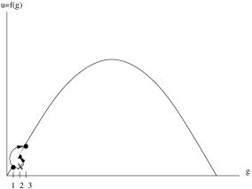
Figure 1.4: The second individual to move must choose between forming a new group of size 2 or joining the existing group of 3. She will choose the group of 3, since it gives her higher utility than the group of 2.

A new group only forms when $f(2)\geq f(g+1)$ where $g$ is the size of the existing large group. The smallest such $g$ is obviously $\bar{g}$, in this case, a group of 17 (Figure 1.5).

Figure 1.5: A new group forms when the large group is size $\bar{g}=17$ because the individual is better off in a new group of size 2.

This is true regardless of how many “large” groups (groups with more than one individual) there are. Thus, the second group forms when there are 83 individuals and one group of 17, the third group forms when there are 69 individuals and two groups of size 17, and so on. The last group forms when there are 15 individuals and five groups of size 17.

This sixth group is the final group that will ever form. Individuals may (and indeed, will) move between the existing groups, but no new group will ever form, because no individual finds it advantageous to move to a group of size 1. The individuals will stop moving when all six groups are approximately the same size–namely, in the configuration with two groups of size 16 and four groups of size 17: $\left\langle 16,16,17,17,17,17\right\rangle$. As predicted by Theorem 2, this is the stable group arrangement with the lowest possible social welfare value. Note also that at no point did we specify the order of play–thus, the players will reach the arrangement $\left\langle 16,16,17,17,17,17\right\rangle$ regardless of their order of motion.

Note that while it is tempting to ascribe this inefficient equilibrium behavior to myopia, that is clearly not all that is at work. It is possible to relax the myopia assumption, and still obtain the same result. Moreover, myopia cannot why individuals would join a group that is already too large. The key to the inefficiency is that when a new member joins a group, her action alters the payoffs of every existing member, creating an externality. When groups are smaller than $g^{*}$, this externality is positive. However, when groups are larger than $g^{*}$, the externality is negative–new members fail to internalize the costs they impose on the incumbent membership. The result of this externality is groups that are much larger than the socially optimal size.

2 Dynamic Group Formation with a Network Constraint

The model of group formation from the previous section assumes that individuals are free to join any existing group, regardless of its current composition. In this section, I consider the effect of social, spacial, and informational constraints on group membership decisions and equilibrium behavior. I model these constraints as an exogenous network of relationships between individuals. An individual cannot join any group to which she is not connected on the network. I then consider the relationship between the structure of the network constraint and the efficiency of the equilibrium outcomes.

2.1 Group Formation with a Network Constraint

Consider a dynamic group formation game, but now, suppose individuals have an exogenous network of connections to other people. An individual can only join a group if it contains a person she is connected to on the network. More formally, $\left(N,f(g),\phi,C\right)$ defines a particular dynamic group formation game with a network constraint, where $C$ is an exogenous, unchanging matrix of connections between individuals–that is, $C_{ij}=1$ if $i$ is connected to $j$ on the network and $0$ otherwise. In this game, an individual’s action set is restricted to include only those groups she is connected to: $A_{i}(t)=\left\{G\,|\,C_{ij}=1\,for\,some\,j\in G\right\}\cup\emptyset\subseteq\pi(t)\cup\emptyset$.

Note that when the network is fully connected, every player knows someone in every group and therefore $A_{i}(t)=\pi(t)\cup\emptyset$. Thus, the unconstrained dynamic group formation game, above, is a special case of the constrained game where the average degree is at a maximum: $\left\langle d\right\rangle=N-1$.

I will also find it convenient to refer to the connections between groups, as well as the connections between individuals: for a network constraint $C$, call two groups, $G_{j}$ and $G_{k}$ connected if $\exists h\in G_{j}$ and $i\in G_{k}$ such that $C_{hi}=1$. That is, two groups are connected if there are individuals in the two groups who are connected on the network, $C$.

2.2 The Set of Stable Configurations with a Network Constraint

As before, the equilibria of the dynamic group formation game must be stable group configurations, which are the Nash equilibria of a static game with the same constraint. An equilibrium of the static game with a network constraint is a partition of the players into groups that is both feasible and individually rational. In particular, $\left(N,f(g),C\right)$ defines a static group formation game with a network constraint. The set of Nash equilibria of this game, $\epsilon\left(N,f\left(g\right),C\right)$, are the set of stable configurations of players into groups, $\left\{G_{1}...G_{J}\right\}$, such that $\forall i$, $i\in G_{j}$ implies:

1. $f\left(g_{j}\right)\geq f\left(g_{k}+1\right)\forall G_{k}\in\left\{G_{1}...G_{J}\right\}$

2. $C_{ij}=1$ for some $j\in G_{j}$

Recall that in the unconstrained case, all stable group configurations share two characteristics: groups are nearly all as large or larger than the social optimum, and all groups larger than the social optimum will be roughly the same size. One result of adding a network constraint is that the there may exist stable group structures in which groups are substantially different sizes.

Claim 3.

For a given static group formation game $\left(N,f(g),C\right)$, there may exist a Nash equilibrium group structure, $\left\{G_{1}...G_{J}\right\}$, such that $\left|g_{j}-g_{k}\right|>1$ for some $g_{j},g_{k}>g^{*}$.

As an illustration of this claim, consider a game with 12 players on a ring. Further suppose $g^{*}=2$ and $\bar{g}=6$, so that all individuals want to be in a group of size 2, and will never form a group larger than size 6. Figure 2.1 illustrates a stable group structure of the static game $\left(N,f(g),C\right)$ with uneven group sizes.

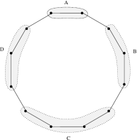
Figure 2.1: An example of an equilibrium group configuration on a ring. Note that this would not be an equilibrium on the fully-connected network because the players in group C would move to group A.

It is obvious from Figure 2.1 how the ring affects the stability of this configuration. The individuals in group C would like to join group A, but they are unable to because they are not connected to that group on the social network. If the network were fully connected, the individuals in group C would like to move to group A, and the configuration would not be stable. Note that the constraint of the ring could represent either a constraint on actions (the players would move if they could) or information (the players would move if they knew). It could also equally well represent an explicit constraint (a legal constraint), an implicit constraint (a social norm), or a functional constraint (a geographic coincidence). This result provides some insight into an empirical puzzle. Our existing models of group formation predict that groups will be the same size in equilibrium. However, empirically, group sizes are clearly far from identical. This model indicates that network-type constraints may be one factor that leads to uneven group sizes.

By exploiting the fact that any two connected individuals form a fully connected subgraph, I can characterize all stable configurations in a group formation game with a network constraint.

Theorem 4.

Let $\left(N,f(g),C\right)$ be a static group formation game with single-peaked payoff function $f(g)$ and network constraint $C$. $\left\{G_{1}...G_{J}\right\}\in\varepsilon\left(N,f(g),C\right)$ if for all connected groups, $G_{j}$ and $G_{k}$, either

1. $g_{j},\,g_{k}\geq g^{*}$ and $|g_{j}-g_{k}|\leq 1$

   or

2. $g_{j}<g^{*}\leq g_{k}$ and $f(g_{k})\geq f(g_{j}+1)\geq f(g_{j})\geq f(g_{k}+1)$

Proof.

Simply note that any pair of connected groups contains a pair of connected agents, who form a fully connected subgraph of the original graph. The result above follows immediately from Theorem 1. ∎

2.3 Equilibrium Behavior

When the players in a group formation game face a binding network constraint, their equilibrium behavior is much more complicated than it is in the unconstrained case. A simple example (see Appendix) shows that Theorem 2 need not hold when there is a network constraint–the set of equilibria may depend on the order of play and there will often be multiple equilibrium group size configurations.

Consider a game with 12 players arranged in a ring, with a single-peaked payoff function, $f(g)$ such that $g^{*}=2$ and $\bar{g}=6$. Now, consider two different orders of motion: $\phi_{1}$ and $\phi_{2}$. For the first order of motion, suppose that the players proceed in order around the ring–that is, $\phi_{1}=$ $\left(1,2,3,4,5,6,7,8,9,10,11,12\right)$. Figure 2.2 shows game play leading to an equilibrium coalition structure with two groups of size 6. A simple analysis indicates that this is the only equilibrium configuration for this order of motion.

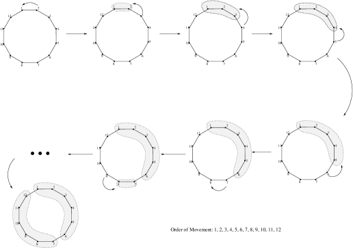
Figure 2.2: In this game, 12 individuals are arranged in a ring. The payoff function, $f(g)$, has maximum $g^{*}=2$ and $\bar{g}=6$. The individuals move in order around the ring–$\phi_{1}=1,2,3,4,5,6,7,8,9,10,11,12$–and wind up in two groups of size 6. In fact, $\left\langle 6,6\right\rangle$ is the only equilibrium group size configuration of the game $\left(12,f(g),\phi_{1}\right)$. Figure 2.3 shows the same game with a different order of play.

Now consider a second game with the same number of players, network constraint, and payoff function, but a different order of play $\phi_{2}=\left(2,3,5,6,8,9,11,12,1,7,4,10\right)$. Figure 2.3 shows one possible sequence of game play, given $\phi_{2}$.

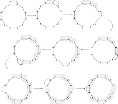
Figure 2.3: This game is identical to the game presented in Figure 2.2 except for the order of motion: $\phi_{2}=2,3,5,6,8,9,11,12,1,7,4,10$. This figure shows a particular sequence of moves, which leads to groups of the ideal size: $\left\langle 3,3,3,3\right\rangle$. Note that $\left\langle 3,3,3,3\right\rangle$ is not an equilibrium of the game presented in Figure 2.2, proving that the set of equilibria may depend on the order of play.

Because the first few players to move are separated from the existing large groups, they are unable to impose on the groups that have already formed, as they did in the previous example. The result is an equilibrium coalition structure with four groups of the ideal size: $\left\langle 3,3,3,3\right\rangle$. Since $\left\langle 3,3,3,3\right\rangle$ is in $\varepsilon\left(N,f(g),\phi_{2},C\right)$ but not in $\varepsilon\left(N,f(g),\phi_{1},C\right)$, it is clear that the order of motion does affect the set of equilibria.

Of course, the outcome pictured in Figure 2.3 is not the only possible equilibrium of the game with order of play $\phi_{2}$. Many players in this game are forced to make random choices. Figure 2.4 shows that if some of those players make different choices, then the players will find themselves in a different configuration–in this case, $\left\langle 4,4,4\right\rangle$.

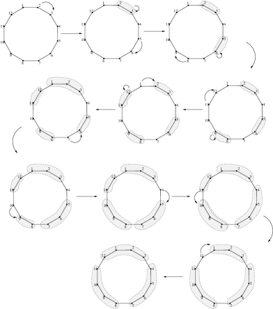
Figure 2.4: This game is identical to that presented in Figure 2.3. Note, in particular, that the order of play is the same: $\phi_{2}=2,3,5,6,8,9,11,12,1,7,4,10$. However, the players have made different random choices, leading to a different equilibrium outcome: $\left\langle 4,4,4\right\rangle$. This shows that when players are sufficiently constrained, there need not be a unique equilibrium coalition size configuration.

Note that when players move according to $\phi_{2}$, the equilibrium behavior produces groups closer to the socially optimal size, and thus a higher social welfare than the equilibrium outcome in the unconstrained game. Thus, imposing the network constraint actually improves equilibrium outcomes.

2.4 Network Structure and Efficiency

Given that equilibrium behavior on a complete network (eg: the unconstrained case) is different than the equilibrium behavior on the ring, one natural question is how the structure of the network constraint will affect the efficiency of the resulting equilibrium, where by efficiency, I mean the fraction of the maximum social welfare captured by the players: $\omega\left(\left\langle g_{1}...g_{J}\right\rangle\right)=\left(\frac{\sum_{j\in\left\langle g_{1}...g_{J}\right\rangle}g_{j}f\left(g_{j}\right)}{Nf\left(g^{*}\right)}\right)$. In particular, I will consider the efficiency of equilibria on a well-studied class of network structures, called Watts-Strogatz networks.

A Watts-Strogatz network is designed to model a wide range of different types of network structures, using only two parameters. It is constructed as follows. One starts with a regular network of degree $d$–this is a network in which every individual is connected to her $\frac{d}{2}$ nearest neighbors on each side. Then each of the links in the regular network is rewired with probability $p$. A link is rewired by disconnecting one end and reconnecting it to a different, random node in the network.

The structure of the Watts-Strogatz network is controlled by adjusting these two parameters: $d$ and $p$. The first, $d$, is the density of the network–the average number of links per person–and it reflects how binding the constraint is (see Figure2.5). On one extreme is a network where everyone is connected to everyone else–where $d=N-1$. As mentioned above, individuals on this network can join any group in the system, so a game on this network is equivalent to the unconstrained case. On the other extreme is a network where no one is connected to anyone else–where $d=0$. In this case, the network is completely disconnected, and nobody can join any group. This is the network constraint at its most binding. The second parameter in the network is the Watts-Strogatz parameter, $p\in\left(0,1\right)$. This parameter indicates what fraction of the links are made at random, and what fraction remain regular (see Figure 2.6). Adjusting this parameter allows me to examine a spectrum of different network types–when $p=0$, the network is regular and approximates a spatial network; when $p=1$, the individuals are connected at random; for values of $p$ between 0 and 1, the network has a “small world” structure, which approximates that of a social network. A pair $\left(d,p\right)$ describes a family of networks with similar topological characteristics.

Figure 2.5: Four different networks with different average degree $\left(d\right)$. Networks with lower degree represent a more binding constraint on group membership decisions.

Figure 2.6: Three networks with different Watts-Strogatz parameters $\left(p\right)$. The Watts-Strogatz network starts with a regular network, where nodes are connected to their two nearest neighbors on each side. Each of these links is rewired at random with probability $p$. Thus, as $p$ increases, the network becomes increasingly random.

Because of the multiplicity of equilibria for a single group formation game, it is necessary to look at the average outcome over a large number of games played on networks with the same values of $d$ and $p$. Players play 1000 group formation games on social networks with the same parameters, $\left(d,p\right)$. I report how close the equilibrium group size vector, $\left\langle g_{1}...g_{J}\right\rangle$, is to being optimal. In particular, I report the fraction of the maximum possible social welfare that the players realize, in equilibrium:

$$\omega\left(\left\langle g_{1}...g_{J}\right\rangle\right)=\left(\frac{\sum_{j\in\left\langle g_{1}...g_{J}\right\rangle}g_{j}f\left(g_{j}\right)}{Nf\left(g^{*}\right)}\right)$$

$\omega=1$ indicates that the players all found themselves in groups of the idea size. Lower values of $\omega$ indicate greater inefficiency.

Here, I present results for a game with logistic payoffs and $g^{*}=10$. The results are the same for other single-peaked payoff functions.

Figure 2.7 illustrates the relationship between the density of the underlying network and the efficiency of the resulting group structure for a random network $\left(p=1\right)$. Since the size of an individual’s action set is bounded above by her degree on the network, degree reflects how constraining the network is on individual behavior. As the degree of the network decreases, the players extract a greater fraction of the maximum possible social welfare. The resulting group structure is more efficient than when the players are unconstrained.

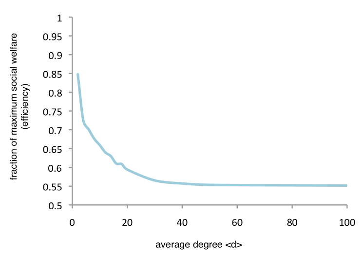
Figure 2.7: Efficiency, as a function of the degree of the network constraint. Individuals form more efficiently-sized groups when constrained by a network of lower degree.

Figure 2.8 shows the effects of the Watts-Strogatz parameter on social welfare. Recall that the Watts-Strogatz parameter, $p$, is the fraction of the links in the network that are made at random. For networks of all degree, the group structure becomes less efficient as the underlying network becomes more random. This is because the more random connections there are, the less binding the network constraint will be for the average individual. When only a small fraction of connections are random, the average individual will tend to know lots of people in the same group. When connections are random, they will know individuals in many different groups, and the constraint will have less bite.

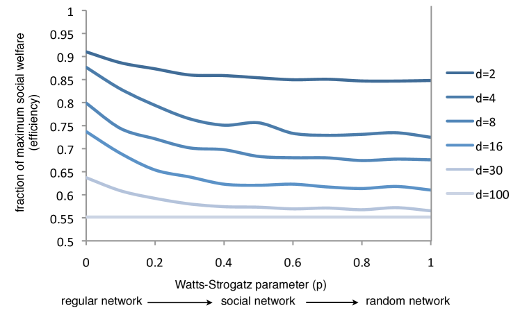
Figure 2.8: Efficiency, as a function of the Watts-Strogatz parameter. The Watts-Strogatz parameter is a measure the amount of order in the network. The group structure is less efficient the more random the underlying network constraint is.

3 Discussion and Conclusion

The equilibrium of the dynamic group formation game is interesting because it is so clearly inefficient–groups become much larger than is socially optimal, even when all individuals agree on the optimum size. Groups become too large because of an externality that new group members impose on existing group members. When a new member joins a group, she alters the utility of all existing group members, creating an externality. When the group is smaller than the social optimum, that externality is positive. However, when the group is the optimal size, the externality is a negative one. The entering member is obviously made better off by joining (otherwise, she would not join), but the rest of the group is made worse off. The negative externality causes individuals to enter a group that does not benefit from the extra member, which then drives groups to become too large. One way to interpret this result is that starting a new group is more difficult than joining an existing, larger group. Thus, there is an incentive to free ride off of early group founders. New groups are under-provided, while existing groups become too large. New groups only form when existing groups become so large that the relatively lower payoffs from starting a new group become worthwhile. Only at that point will groups splinter.

I have shown that the social, spacial, and informational constraints faced by individuals making group membership decisions will improve the efficiency of the resulting group structure. Initially, it might be surprising that restricting individuals by forcing them to choose groups that they have a connection to would improve outcomes. However, this is consistent with the fact that the inefficiency in the unconstrained case is due to a negative externality. When players are constrained by social, spacial, and informational networks, they do not always have access to established groups and are forced to form new groups, rather than joining groups that are already too large. In other words, the network constraint limits the players’ choice sets, which forces them to internalize the start up costs of creating a new group, limiting their ability to impose a negative externality on others.

There is a clear relationship between the structure of the network constraint and the equilibrium group structure. The players form into more efficient groups when they are constrained by networks that have lower density (lower average degree, $d$) and are more ordered and less random (smaller fraction of random links, $p$). Both of these aspects of network topology affect how binding the network constraint is. A network with lower average degree means that individuals on the network will be connected to fewer groups on average, restricting their action set and making the network constraint more binding. Similarly, when there are few random connections in the network, the average individual will have access to fewer distinct groups, making the network constraint bind. This suggests that group structures will be more efficient when group membership requires a stronger relationship (implying a network of lower density). Moreover, given that social networks have more random links than spacial networks, we would expect groups to be closer to the ideal size when group membership is constrained by geography, rather than social connections.

4 Appendix:

4.1 Proof of the Static Game Equilibrium

Theorem 1 is built up from three lemmas. The first lemma states that in any static equilibrium, at most one group will be smaller than the socially optimal size. The second lemma states that all groups larger than the optimum will be the same size, up to integer constraints. The third lemma pins down the size of any group smaller than the optimum.

Lemma 5.

Let $\left(N,f(g)\right)$ be a static group formation game with $f(g)$ single-peaked. Then $\exists$ no equilibrium $\left\langle g_{1}...g_{J}\right\rangle\in\varepsilon\left(N,f(g)\right)$ such that $g_{i}\leq g_{j}<g^{*},\,i\neq j$. That is, in equilibrium at most one group will be smaller than the social optimum.

Proof.

Towards a contradiction, suppose $\exists\left\langle g_{1}...g_{J}\right\rangle\in\varepsilon\left(N,f(g)\right)$ such that $g_{1}\leq g_{2}<g^{*}$. $f(.)$ is strictly increasing in that range, so $f(g_{1})<f(g_{2}+1)$. But then players in group 1 have an incentive to move to group 2, so $\left\langle g_{1}...g_{J}\right\rangle$ cannot be an equilibrium ∎

Lemma 5 implies that in characterizing $\varepsilon\left(N,f(g)\right)$, we need consider only two cases: either all of the groups are larger than the socially optimal size ($g_{1}...g_{k}\geq g$), or exactly one group is small ($g_{1}<g^{*}$and $g_{2}...g_{k}\geq g^{*}$). The following two Lemmas address the sizes of the groups in these two different cases. Lemma 6 shows that in any equilibrium where all groups are larger than the social optimum, the groups must be approximately the same size. Lemma 7 sets a more restrictive condition in the case where one group is smaller than the social optimum.

Lemma 6.

Let $\left(N,f(g)\right)$ be a static group formation game with $f(g)$ single-peaked. Then for all $\left\langle g_{1}...g_{J}\right\rangle\in\varepsilon\left(N,f(g)\right)$, $|g_{i}-g_{j}|\leq 1\,$$\forall g_{i},g_{j}\geq g^{*}$. That is, in equilibrium, all groups larger than the social optimum must be the same size, up to integer constraints.

Proof.

Towards a contradiction, suppose $\exists\left\langle g_{1}...g_{J}\right\rangle\in\varepsilon\left(N,f(g)\right)$ such that $g_{1}>g_{2}\geq g^{*}$ and $g_{1}-g_{2}>1$. $f(.)$ is strictly decreasing in this range, so $f(g_{1})<f(g_{2}+1)$ But then players in group 1 have an incentive to move to group 2, so $\left\langle g_{1}...g_{J}\right\rangle$ cannot be an equilibrium.

Note that this result extends a result in Nitzen (1991) to the case of single-peaked utility. Arnold and Wooders (2005) prove a similar result for a sequential game. The following lemma extends that result to the case where one group is smaller than the social optimum. The Nash Equilibrium requires a slightly stronger restriction on the size of the groups.∎

Lemma 7.

Let $\left(N,f(g)\right)$ be a static group formation game with $f(g)$ single-peaked. Then for all $\left\langle g_{1}...g_{J}\right\rangle\in\varepsilon\left(N,f(g)\right)$ such that $g_{1}<g^{*}$, both of the following must be true:

1. $f(g_{j})\geq f(g_{1}+1)\geq f(g_{1})\geq f(g_{j}+1)\,\forall\,j>1$

2. $g_{j}=g_{k}\,\forall\,j,k\neq 1$

Proof.

Let $\left\langle g_{1}...g_{J}\right\rangle\in\varepsilon\left(N,f(g)\right)$such that $g_{1}<g^{*}$.

Part 1: Consider group 1 (the small coalition) and an arbitrary group $j$, such that $g_{j}\geq g^{*}$ Note that $f(g_{1})<f(g_{1}+1)$ and $f(g_{j})>f(g_{j}+1)$. If $f(g_{1})<f(g_{j}+1)$, then players in group 1 would move to group $k$. Similarly, if $f(g_{j})<f(g_{1}+1)$, then players in group $k$ would move to group 1. Together, these three inequalities imply $f(g_{j})\geq f(g_{1}+1)\geq f(g_{1})\geq f(g_{j}+1)\,\forall\,j>1$

Part 2: consider two arbitrary groups, $j$ and $k$, such that $g_{k}\geq g_{j}\geq g^{*}$. Lemma 6 indicates that $g_{k}-g_{j}\leq 1$. Towards a contradiction, suppose $g_{k}-g_{j}=1$, so that $g_{k}=g_{j}+1$. By Part 1, $f(g_{j}+1)\leq f(g_{1})$. Since we assumed $g_{k}=g_{j}+1$, this implies that $f(g_{k})\leq f(g_{1}).$ But since $f(g_{1})<f(g_{1}+1)$ to the left of the optimum, $f(g_{k})<f(g_{1}+1)$, meaning that players in group $j$ would move to group $k$. Thus, it must be that $g_{j}=g_{k}$ exactly. ∎

Together, the restrictions imposed by these three lemmas form the basis of Theorem 1.

4.2 Proof of multiple stable configurations

Theorem 8 puts a lower bound on the number of equilibria in the set $\varepsilon\left(N,f(g)\right)$, showing that there the static game has multiple equilibria, meaning that there will be multiple stable group configurations.

Theorem 8.

Let $\left(N,f(g)\right)$ be a static group formation game. Then $\left|\varepsilon\left(N,f(g)\right)\right|\geq\frac{N}{g^{*}}-\frac{N}{\bar{g}}-1$.

Proof.

I will set the lower bound by enumerating the equilibria in which all groups are larger than the social optimum (ie: the first set in Theorem 1). Note that since all groups are approximately the same size, each equilibrium with all large groups is entirely characterized by the number of groups. The largest possible group is $\bar{g}$ and the smallest possible group is $g^{*}$. Thus, there should be one equilibrium for each integer in the interval $\left[\frac{N}{\bar{g}},\frac{N}{g^{*}}\right]$, or $\frac{N}{g^{*}}-\frac{N}{\bar{g}}-1$. ∎

Since the lower bound in Theorem 8 is usually greater than 1, the static game will usually have multiple equilibria.

5 Acknowledgements

Thanks to Scott Page, Rick Riolo, Robert Willis, Lada Adamic, and Ross O’Connell. This work was done with the support of the NSF. Computing resources provided by the University of Michigan Center for the Study of Complex Systems.

References

- (1)
- Arnold and Wooders (2005) Arnold, Tone and Myrna Wooders, “by Dynamic Club Formation with Coordination,” 2005.
- Arnold and Schwalbe (2002) and Ulrich Schwalbe, “Dynamic coalition formation and the core,” Journal of Economic Behavior & Organization, 2002, 49 (3), 363–380.
- Bloch (1996) Bloch, Francis, “Sequential Formation of Coalitions in Games with Externalities and Fixed Payoff Division,” Games and Economic Behavior, 1996, 14 (1), 90–123.
- Bloch (2010) , “Formation of Networks and Coalitions,” Handbook of Social Economics J Benhabib A, 2010, Volume 1 (January), 729–779.
- Copic et al. (2009) Copic, Jernej, Matthew O Jackson, and Alan Kirman, “Identifying Community Structures from Network Data via Maximum Likelihood Methods,” The BE Journal of Theoretical Economics, 2009, 9 (1), 1–39.
- Demange and Wooders (2005) Demange, Gabrielle and Myrna H. Wooders, Group formation in economics: networks, clubs and coalitions, Cambridge University Press, 2005.
- Girvan and Newman (2002) Girvan, M and M E J Newman, “Community structure in social and biological networks.,” Proceedings of the National Academy of Sciences of the United States of America, June 2002, 99 (12), 7821–6.
- Hart and Kurz (1983) Hart, S and M Kurz, “Endogenous formation of coalitions,” 1983.
- Heintzelman et al. (2009) Heintzelman, Martin D, Stephen W Salant, and Stephan Schott, “Putting free-riding to work: A Partnership Solution to the common-property problem,” Journal of Environmental Economics and Management, 2009, 57 (3), 309–320.
- Jackson (2008) Jackson, Matthew O., Social and Economic Networks, Princeton University Press, 2008.
- Konishi and Ray (2003) Konishi, Hideo and Debraj Ray, “Coalition formation as a dynamic process,” Journal of Economic Theory, 2003, 110 (1), 1–41.
- Konishi et al. (1997) , Michel Le Breton, and Shlomo Weber, “Pure Strategy Nash Equilibrium in a Group Formation Game with Positive Externalities,” Games and Economic Behavior, October 1997, 21 (1-2), 161–182.
- Macho-Stadler et al. (2006) Macho-Stadler, Inés, David Pérez-Castrillo, and Nicolás Porteiro, “Sequential Formation of Coalitions Through Bilateral Agreements in a Cournot Setting,” International Journal of Game Theory, 2006, 34 (2), 207–228.
- Newman and Girvan (2003) Newman, M E J and M Girvan, “Finding and evaluating community structure in networks,” Physical Review E - Statistical, Nonlinear and Soft Matter Physics, 2003, 69 (2 Pt 2), 16.
- Nitzan (1991) Nitzan, Shmuel, “Collective Rent Dissipation,” The Economic Journal, 1991, 101 (409), 1522–1534.
- Page and Wooders (2007) Page, Frank H and Myrna Wooders, “Networks and clubs,” Journal of Economic Behavior & Organization, 2007, 64 (3–4), 406–425.
- Watts and Strogatz (1998) Watts, Duncan J and Steven H Strogatz, “Collective dynamics of ’small-world’ networks.,” Nature, 1998, 393 (6684), 440–2.
- Yi and Shin (2000) Yi, Sang-Seung and Hyukseung Shin, “Endogenous formation of research coalitions with spillovers,” International Journal of Industrial Organization, 2000, 18 (2), 229–256.