${\rm O}(a)$ improvement of the HYP static axial and vector currents at one-loop order of perturbation theory

Abstract:

We calculate analytically the improvement coefficients of the static axial and vector currents in ${\rm O}(a)$ improved lattice QCD at one-loop order of perturbation theory. The static quark is described by the hypercubic action, previously introduced in the literature in order to improve the signal-to-noise ratio of static observables. Within a Schrödinger Functional setup, we derive the Feynman rules of the hypercubic link in time-momentum representation. The improvement coefficients are obtained from on-shell correlators of the static axial and vector currents. As a by-product, we localise the minimum of the static self-energy as a function of the smearing parameters of the action at one-loop order and show that the perturbative minimum is close to its non-perturbative counterpart.

1 Introduction

The hypercubic (HYP) link has been introduced a few years ago in order to study the static quark/anti-quark potential with improved statistical precision [1]. In this context it proved to be remarkably effective at large quark distances, where a description of the static propagators in terms of thin gauge links was known to lead to an excessive noise. The origin of the statistical improvement has been subsequently identified as due to a strong reduction of the static self-energy for appropriate choices of the HYP smearing parameters [2].

Since the binding energy of static mesons is amplified by self-energy contributions, the adoption of the HYP link as a parallel transporter in the static action, originally introduced in ref. [3], has allowed for lattice simulations with smaller binding potentials, thus triggering an exponential improvement of the signal-to-noise ratio of meson correlators at large time distances. This helped significantly in several applications of Heavy Quark Effective Theory (HQET) [4, 5, 6, 7, 8, 9].

On a theoretical side, the HYP smearing procedure looks superior to other techniques in that it mixes gauge links within hypercubes attached to the original link only, which allows to preserve locality to a high degree.

In spite of the statistical gain, the HYP link brings on an increase of operational complexity, which in some applications has compelled to resort to approximations. For instance, this is the case with the ${\rm O}(a)\$improvement of the static-light bilinear operators, which has been addressed to in [2, 10]. In these papers the improvement of the static axial and vector currents is obtained by imposing that on-shell renormalised correlators of the currents with different choices of the HYP smearing parameters differ by ${\rm O}(a^{2})\$effects. Obviously, this procedure allows to relate the operator improvement coefficients corresponding to different static discretisations, but in order to isolate all of them, the improvement coefficients must be known for at least one choice of the smearing parameters.

An approximate solution has been obtained by using a one-loop perturbative evaluation of the improvement coefficients with static discretisations characterised by simpler lattice Feynman rules, such as the original Eichten-Hill (EH) one or the so-called APE discretisation (see [2] and sect. 2 for definitions). The approximate solutions thus obtained for other choices of the HYP parameters are therefore affected by ${\rm O}(g_{0}^{4})$ systematic errors. As such, they have to be regarded as effective estimates, which are neither purely one-loop perturbative, nor fully non-perturbative. Of course, the amount of the ${\rm O}(g_{0}^{4})$ terms can be assessed only if the one-loop value of such improvement coefficients is known exactly.

The aim of the present paper is precisely the analytical determination of the improvement coefficients of the static axial and vector currents at one-loop order of perturbation theory (PT) for the most convenient choices of the HYP link. In order to accomplish this, we adopt a formalism based on the Schrödinger Functional (SF) [12, 13], derive the lattice Feynman rules of the HYP link at one-loop order of PT in time-momentum representation, and follow [10, 11] as for the choice of the operator improvement conditions.

As a by-product, we also calculate the static self-energy at one-loop order as a function of the smearing parameters and perform a numerical minimisation of it. Remarkably, the minimum of the self-energy is found for a choice of the smearing parameters which is very close to what is nowadays called the HYP2 action [2], thus showing that the self-energy is dominated by perturbation theory.

The paper is organised as follows. In sect. 2 we review some basic definitions and introduce our notation for the HYP static action. Sect. 3 is devoted to a discussion of the effects of the SU(3) projection, used in the HYP procedure, at one-loop order of PT; we show that some results, previously known in the literature, are largely independent of how the projection is defined. In sect. 4 we provide a simple derivation of the Feynman rules of the temporal HYP link in time-momentum representation. A systematic study of the one-loop static self-energy is described in sect. 5. In sect. 6 we collect our results for the improvement coefficients. Conclusions are drawn in sect. 7. For the sake of readability we strived to avoid as much as possible unessential technicalities. For this reason, algebraic details have been almost completely confined to the appendices.

2 Notation and basic definitions

2.1 HYP static action

In order to set-up the notation, we review some basic formulae concerning the static theory and the HYP link. Static quarks are represented by a pair of fermion fields $(\psi_{\rm\phantom{\bar{h}^{\dagger}}h},\psi_{{\rm\phantom{\bar{h}^{\dagger}}\bar{h}}})$, propagating forward and backward in time, respectively; their dynamics is governed by the lattice action [3]

$$S^{\rm stat}[\psi_{\rm\phantom{\bar{h}^{\dagger}}h},\psi_{{\rm\phantom{\bar{h}^{\dagger}}\bar{h}}}]=a^{4}\sum_{x}\left[{\overline{\psi}}_{\rm h}(x)\nabla_{0}^{*}\psi_{\rm\phantom{\bar{h}^{\dagger}}h}(x)-\overline{\psi}_{\bar{\rm h}}(x)\nabla_{0}\psi_{{\rm\phantom{\bar{h}^{\dagger}}\bar{h}}}(x)\right],$$ (1)

where the forward and backward covariant derivatives $\nabla_{0},\,\nabla_{0}^{*}$ are defined via

$$\nabla_{0}\psi_{{\rm\phantom{\bar{h}^{\dagger}}\bar{h}}}(x)=\frac{1}{a}\left[W_{0}(x)\psi_{{\rm\phantom{\bar{h}^{\dagger}}\bar{h}}}(x+a\hat{0})-\psi_{{\rm\phantom{\bar{h}^{\dagger}}\bar{h}}}(x)\right],$$

$$\nabla_{0}^{*}\psi_{\rm\phantom{\bar{h}^{\dagger}}h}(x)=\frac{1}{a}\left[\psi_{\rm\phantom{\bar{h}^{\dagger}}h}(x)-W_{0}(x-a\hat{0})^{-1}\psi_{\rm\phantom{\bar{h}^{\dagger}}h}(x-a\hat{0})\right].$$ (2)

The field $\psi_{\rm\phantom{\bar{h}^{\dagger}}h}$(${\overline{\psi}}_{\rm h}$) can be thought of as the annihilator(creator) of a heavy quark. Similarly, $\psi_{{\rm\phantom{\bar{h}^{\dagger}}\bar{h}}}$($\overline{\psi}_{\bar{\rm h}}$) creates(annihilates) a heavy anti-quark. Each field is represented by a four-component Dirac vector, yet only half of the components play a dynamical rôle, owing to the static projection constraints

$$P_{\scriptscriptstyle+}\psi_{\rm\phantom{\bar{h}^{\dagger}}h}=\psi_{\rm\phantom{\bar{h}^{\dagger}}h}\ ,\qquad{\overline{\psi}}_{\rm h}P_{\scriptscriptstyle+}={\overline{\psi}}_{\rm h}\ ,\qquad P_{\scriptscriptstyle+}=\frac{1}{2}(11+\gamma_{0})\ ;$$

$$P_{\scriptscriptstyle-}\psi_{{\rm\phantom{\bar{h}^{\dagger}}\bar{h}}}=\psi_{{\rm\phantom{\bar{h}^{\dagger}}\bar{h}}}\ ,\qquad\overline{\psi}_{\bar{\rm h}}P_{\scriptscriptstyle-}=\overline{\psi}_{\bar{\rm h}}\ ,\qquad P_{\scriptscriptstyle-}=\frac{1}{2}(11-\gamma_{0})\ .$$ (3)

The static action has a functional dependence upon the parallel transporter $W_{0}$, which is assumed to be represented in this paper by a temporal HYP link. According to the original definition [1], the HYP link is obtained through a three-step recursive smearing procedure, where the original thin link is decorated with staples belonging to its surrounding hypercube, i.e.

$$W_{\mu}(x)\equiv W^{(3)}_{\mu}(x) ={{\cal P}}_{\rm\scriptscriptstyle SU(3)}[(1-\alpha_{1})U_{\mu}(x)+$$

$$+\frac{\alpha_{1}}{6}\sum_{\pm\nu\neq\mu}W^{(2)}_{\nu;\mu}(x)W^{(2)}_{\mu;\nu}(x+a\hat{\nu})W^{(2)}_{\nu;\mu}({x+a\hat{\mu}})^{\dagger}]\,,$$ (4)

$$W^{(2)}_{\mu;\nu}(x) ={{\cal P}}_{\rm\scriptscriptstyle SU(3)}[(1-\alpha_{2})U_{\mu}(x)+$$

$$+\frac{\alpha_{2}}{4}\sum_{\pm\rho\neq\nu,\mu}W^{(1)}_{\rho;\nu\mu}(x)W^{(1)}_{\mu;\rho\nu}(x+a\hat{\rho})W^{(1)}_{\rho;\nu\mu}(x+a\hat{\mu})^{\dagger}]\,,\hfill$$ (5)

$$W^{(1)}_{\mu;\nu\rho}(x) ={{\cal P}}_{\rm\scriptscriptstyle SU(3)}[(1-\alpha_{3})U_{\mu}(x)+$$

$$+\frac{\alpha_{3}}{2}\sum_{\pm\eta\neq\rho,\nu,\mu}U_{\eta}(x)\ U_{\mu}(x+a\hat{\eta})U_{\eta}(x+a\hat{\mu})^{\dagger}]\,,$$ (6)

where $U_{-\mu}(x)=U^{\dagger}_{\mu}(x-a\hat{\mu})$. In Eq. (2.1) $U_{\mu}$ denotes the fundamental gauge link and the index $\nu$ in $W^{(2)}_{\mu;\nu}$ indicates that the fat link at location $x$ and direction $\mu$ is not decorated with staples extending in direction $\nu.$ The decorated link $W^{(2)}_{\mu;\nu}$ is then constructed in Eq. (2.1) with a modified APE blocking from another set of decorated links, where the indices $\rho\,\nu$ indicate that the fat link $W^{(1)}_{\mu;\rho\,\nu}$ in direction $\mu$ is not decorated with staples extending in the $\rho$ or $\nu$ directions. Finally, the decorated link $W^{(1)}_{\mu;\rho\,\nu}$ is constructed in Eq. (2.1) from the original thin links with a modified APE blocking step where only the two staples orthogonal to $\mu,\,\nu$ and $\rho$ are used. After each smearing step, the new fat link is projected onto SU(3). Popular choices of the smearing parameters are represented by

$$\rm{EH}\ : \hskip 56.9055pt(\alpha_{1},\alpha_{2},\alpha_{3})\,=\,(\ \,0.0,\ \,0.0,\ \,0.0)\ ,$$ (7)

$$\rm{HYP1}\ : \hskip 56.9055pt(\alpha_{1},\alpha_{2},\alpha_{3})\,=\,(0.75,\ \,0.6,\ \,0.3)\ ,$$ (8)

$$\rm{HYP2}\ : \hskip 56.9055pt(\alpha_{1},\alpha_{2},\alpha_{3})\,=\,(\ \,1.0,\ \,1.0,\ \,0.5)\ .$$ (9)

The APE action of ref. [2] is characterised by a parallel transporter, which is not projected onto SU(3). Therefore, the action cannot be generated through a HYP link for any choice of the smearing parameters at a non-perturbative level. Nevertheless, the SU(3) projection is irrelevant at one-loop order of PT, as shown in next section. It follows that, as far as we are concerned here, the APE action is obtained from

$$\rm{APE}\ : \hskip 56.9055pt(\alpha_{1},\alpha_{2},\alpha_{3})\,=\,(1.0,\ \,0.0,\ \,0.0)\ .$$ (10)

2.2 ${\rm O}(a)\$improvement of the static currents

We adopt a SF topology where periodic boundary conditions (up to a phase $\theta$ for the light quark fields) are set up on the spatial directions and Dirichlet boundary conditions are imposed on time at $x_{0}=0,T$. We also assume no background field in our theory. The SF formalism has certain advantages, which have been widely discussed in the literature; we refer the reader to [14] for an introduction to the subject. In particular, it is here adopted since it allows for an easy on-shell formulation of the improvement problem.

In this paper, we are interested in the static axial and vector currents

$$A_{0}^{\rm stat}(x) =\overline{\psi}(x)\gamma_{0}\gamma_{5}\psi_{\rm\phantom{\bar{h}^{\dagger}}h}(x)\ ,$$ (11)

$$V_{0}^{\rm stat}(x) =\overline{\psi}(x)\gamma_{0}\psi_{\rm\phantom{\bar{h}^{\dagger}}h}(x)\ .$$ (12)

The ${\rm O}(a)\$improvement of these operators with Wilson light and EH static quarks has been studied at one-loop order of PT in [10, 11]. The general improvement pattern is as follows:

$$(A_{\rm\scriptscriptstyle R}^{\rm stat})_{0} ={Z^{\rm stat}_{\rm\scriptscriptstyle A}}(1+{b^{\rm stat}_{\rm\scriptscriptstyle A}}am_{\rm q})(A_{\rm\scriptscriptstyle I}^{\rm stat})_{0}\ ,$$ (13)

$$(V_{\rm\scriptscriptstyle R}^{\rm stat})_{0} ={Z^{\rm stat}_{\rm\scriptscriptstyle V}}(1+{b^{\rm stat}_{\rm\scriptscriptstyle V}}am_{\rm q})(V_{\rm\scriptscriptstyle I}^{\rm stat})_{0}\ ,$$ (14)

with

$$(A_{\rm\scriptscriptstyle I}^{\rm stat})_{0} =A_{0}^{\rm stat}+a{c^{\rm stat}_{\rm\scriptscriptstyle A}}\delta A_{0}^{\rm stat}\ ,\qquad \quad\delta A_{0}^{\rm stat}(x) =\overline{\psi}(x)\gamma_{j}\gamma_{5}\frac{1}{2}\left(\overleftarrow{\nabla}_{j}+\overleftarrow{\nabla}^{*}_{j}\right)\psi_{\rm\phantom{\bar{h}^{\dagger}}h}(x)\ ;$$ (15)

$$(V_{\rm\scriptscriptstyle I}^{\rm stat})_{0} =V_{0}^{\rm stat}+a{c^{\rm stat}_{\rm\scriptscriptstyle V}}\delta V_{0}^{\rm stat}\ ,\qquad \quad\delta V_{0}^{\rm stat}(x) =\overline{\psi}(x)\gamma_{j}\frac{1}{2}\left(\overleftarrow{\nabla}_{j}+\overleftarrow{\nabla}^{*}_{j}\right)\psi_{\rm\phantom{\bar{h}^{\dagger}}h}(x)\ .$$ (16)

The improvement coefficients ${c^{\rm stat}_{\rm\scriptscriptstyle A}}$, ${c^{\rm stat}_{\rm\scriptscriptstyle V}}$, ${b^{\rm stat}_{\rm\scriptscriptstyle A}}$ and ${b^{\rm stat}_{\rm\scriptscriptstyle V}}$ depend on the gauge coupling and are perturbatively expanded according to

$$c_{\rm\scriptscriptstyle X}^{\rm stat} =c_{\rm\scriptscriptstyle X}^{{\rm stat}(1)}g_{0}^{2}+{\rm O}(g_{0}^{4})\ ,\qquad$$ (17)

$$b_{\rm\scriptscriptstyle X}^{\rm stat} =\frac{1}{2}+b_{\rm\scriptscriptstyle X}^{{\rm stat}(1)}g_{0}^{2}+{\rm O}(g_{0}^{4})\ ;\qquad \qquad{\rm X}={\rm A,V}\ .$$ (18)

We do not review explicitely the improvement conditions used in [10, 11] here, but perform the same perturbative analysis with HYP action and refer the reader to those papers for details. In particular, we extract the one-loop improvement coefficients ${c^{\rm stat(1)}_{\rm\scriptscriptstyle A}}$ and ${b^{\rm stat(1)}_{\rm\scriptscriptstyle A}}$ of the static axial current as explained in appendix B of [11], and the one-loop improvement coefficients ${c^{\rm stat(1)}_{\rm\scriptscriptstyle V}}$ and ${b^{\rm stat(1)}_{\rm\scriptscriptstyle V}}$ of the static vector current according to Eqs. (4.3)-(6.13) of [10].

3 ${\rm SU}(3)$ projection at one-loop order of PT

The ${\rm SU}(3)$ projector ${{\cal P}}_{\rm\scriptscriptstyle SU(3)}$ is not uniquely defined and the resulting HYP link depends in principle upon the chosen definition. Here we follow [2]: if $A$ denotes a generic $3\times 3$ complex matrix, its projection $M$ onto SU(3) is defined by

$$M=\frac{X}{\sqrt[3]{(\det{X})}}\ ,\qquad X={\ A}({{A^{\dagger}A}})^{-1/2}\ ,$$ (19)

i.e. the matrix $A$ is first unitarised, and then its determinant is rotated to one. Another very popular definition goes through the maximisation (minimisation) of the real (imaginary) part of ${\rm tr}({M^{\dagger}A})$. The latter has been employed in particular in [15], where two valuable propositions have been proved, which allow for a substantial simplification of perturbative calculations at one-loop order. The propositions concern the adjoint field of the HYP link, when this is expanded in power series of the adjoint (gluon) field of the fundamental gauge link. They read as follows:

• the linear term of the series is invariant under the action of ${{\cal P}}_{\rm\scriptscriptstyle SU(3)}$;

• the quadratic term is anti-symmetric in the gluon field.

Although the proof proposed in [15] is based on the specific definition of the SU(3) projector as $\max_{M}\{{\rm Re\,tr}[M^{\dagger}A]\}$, the above statements hold as well if Eq. (19) is adopted instead. A proof of this is straightforward. To fix the notation, we define the gauge field $q_{\mu}^{a}(x)$ of the fundamental link via

$$U_{\mu}(x)=\exp\{ag_{0}q_{\mu}^{a}(x)T^{a}\}\ ,$$ (20)

where $\{T^{a}\}_{a=1\dots 8}$ denotes an anti-hermitian representation of the Gell-Mann matrices. Following [15], the unprojected APE-blocked links of Eqs. (2.1)–(2.1) are written in the general form

$$V_{\mu}(x)=11\ +\ ag_{0}\sum_{\nu;y}f_{\mu\nu}(x,y)q_{\nu}(y)\ +\ a^{2}g_{0}^{2}\sum_{\nu\rho;yz}h_{\mu\nu\rho}(x,y,z)q_{\nu}(y)q_{\rho}(z)\ +\ {\rm O}(g_{0}^{3})\ ,$$ (21)

with real vertices $f,h$ depending on the level of the HYP smearing and $q_{\mu}(x)=q_{\mu}^{a}(x)T^{a}$. It should be observed that, since $V_{\mu}$ is neither a ${\rm SU}(3)$ nor a ${\rm U}(3)$ matrix, no gauge field can be associated with it. Projecting the link according to Eq. (19) leads to

$${V_{\mu}(x)}\left[{{V^{\dagger}_{\mu}(x)V_{\mu}(x)}}\right]^{-1/2}\ =\ 11 \ +\ ag_{0}\sum_{\nu;y}f_{\mu\nu}(x,y)q_{\nu}(y)$$

$$\ +\ \frac{a^{2}g_{0}^{2}}{2}\sum_{\nu\rho;yz}h_{\mu\nu\rho}(x,y,z)[q_{\nu}(y),q_{\rho}(z)]$$

$$\ +\ \frac{a^{2}g_{0}^{2}}{2}\sum_{\nu\rho;yz}f_{\mu\nu}(x,y)f_{\mu\rho}(x,z)q_{\nu}(y)q_{\rho}(z)$$

$$\ +\ {\rm O}(g_{0}^{3})\ ,$$ (22)

and

$$\det\left\{{V_{\mu}(x)}\left[{{V^{\dagger}_{\mu}(x)V_{\mu}(x)}}\right]^{-1/2}\right\}\ =\ 1\ +\ {\rm O}(g_{0}^{3})\ .$$ (23)

Eq. (23) can been easily checked through an algebraic program, such as FORM [16]. The projected link ${\cal P}_{\rm\scriptscriptstyle SU(3)}[V_{\mu}(x)]$ is now in ${\rm SU}(3)$ by construction. Consequently, we are allowed to introduce a smeared gauge field

$${\cal P}_{\rm\scriptscriptstyle SU(3)}[V_{\mu}(x)]=\exp\{ag_{0}v_{\mu}^{a}(x)T^{a}\}\ .$$ (24)

As a remark we also note that, since the perturbative expansion of the staples generates gauge fields at all orders in PT, $v_{\mu}$ cannot be assumed as a linear function of $q_{\mu}$, and has to be perturbatively expanded in its turn, i.e.

$$v_{\mu}=v^{\prime}_{\mu}\ +\ ag_{0}v^{\prime\prime}_{\mu}\ +\ {\rm O}(g_{0}^{2})\ .$$ (25)

Accordingly, Eq. (24) reads

$${\cal P}_{\rm\scriptscriptstyle SU(3)}[V_{\mu}(x)]=11\ +\ ag_{0}v^{\prime}_{\mu}\ +\ a^{2}g_{0}^{2}v^{\prime\prime}_{\mu}\ +\ \frac{a^{2}g_{0}^{2}}{2}v^{\prime}_{\mu}v^{\prime}_{\mu}\ +\ {\rm O}(g_{0}^{3})\ .$$ (26)

Equating Eq. (3) and Eq. (26) order by order in the bare coupling allows to express the smeared gauge field in terms of the unsmeared one. In particular

$${\rm O}(g_{0}^{0}):\qquad 11\ =\ 11\ ,\hskip 142.26378pt$$ (27)

$${\rm O}(g_{0}^{1}):\qquad v^{\prime}_{\mu}\ =\ \sum_{\nu;y}f_{\mu\nu}(x,y)q_{\nu}(y)\ ,$$ (28)

$${\rm O}(g_{0}^{2}):\qquad \ v^{\prime\prime}_{\mu}\ =\ \frac{1}{2}\sum_{\nu\rho;yz}h_{\mu\nu\rho}(x,y,z)[q_{\nu}(y),q_{\rho}(z)]\ .$$ (29)

Eqs. (28)–(29) correspond precisely to propositions 1 and 2 of [15]. It is worth noting that tadpole diagrams associated with Eq. (29) do not contribute to any one-loop perturbative calculation in absence of a background field, although they are ${\rm O}(g_{0}^{2})$. Indeed, the commutator $[T^{a},T^{b}]=-f^{abc}T^{c}$ is anti-symmetric in $a\leftrightarrow b$, while the Wick contraction $\langle q^{a}q^{b}\rangle$ is symmetric. Nevertheless, one should avoid the conclusion that tadpoles do not contribute at all, because terms such as $v^{\prime}_{\mu}(x)v^{\prime}_{\mu}(x)$ have to be always considered. Moreover, the vanishing of the above-mentioned contributions is not anymore true in presence of a background field, where PT becomes more cumbersome.

To summarise, Eqs. (28)–(29) show that the smeared gauge field can be taken as a linear function of the unsmeared one at one-loop in PT and zero background field. The effect of the ${\rm SU}(3)$ projection can be disregarded in the linear term, and non-linear contributions should be discarded when deriving the Feynman rules of the HYP link.

4 Feynman rules in time-momentum representation

Translational invariance along time is broken within the SF formalism. This fact complicates perturbation theory, which is usually worked out in momentum space, and makes it natural to adopt a mixed approach, known as time-momentum representation, where only the spatial coordinates are Fourier transformed. Accordingly, tree-level propagators and interaction vertices are functions of time and spatial momenta.

We derive the Feynman rules in time-momentum representation for the temporal component of the HYP link according to two different and independent procedures. The first derivation makes use of the results obtained in full momentum space [17] and arrives at time-momentum representation by inverse Fourier transform in time. This is possible in presence of homogeneous Dirichlet boundary conditions, which allow to continue the SF periodically to all times with no non-trivial terms at the boundaries. The second derivation follows by direct construction upon representing the HYP smearing as a lattice differential operator acting linearly on the fundamental gauge fields. In this section we report only the first derivation; the second one, which is quite lengthy, is sketched in appendix A. For the sake of completeness, we report in appendix B the Feynman rules in time-momentum representation for the spatial components of the HYP link, which may be useful for some applications of HQET (e.g. see ref. [5]) and for dynamical n-HYP [18].

In order to fix the notation, we define the smeared gauge fields of the three levels of the HYP procedure according to

$$W^{(k)}_{\mu}(x) =\exp\{ag_{0}B^{(k)}_{\mu}(x)\}\ ,\qquad\qquad k=1,2,3\ .$$ (30)

Under the assumption of periodic boundary conditions in space and homogenous Dirichlet ones in time without nontrivial boundary terms in the action, the gauge field of the fundamental (and smeared) link admits a 4-dimensional Fourier transform

$$q_{\mu}(x)=\frac{1}{L^{4}}\sum_{p}{\rm e}^{ipx}{\rm e}^{i\frac{a}{2}p_{\mu}}\tilde{q}_{\mu}(p)\ ,\qquad-\frac{\pi}{a}\leq p_{\mu}=\frac{2\pi}{L}n_{\mu}<\frac{\pi}{a}\ ,$$ (31)

where $L$ is the toroidal extension of the space-time dimensions and the additional phase shift in direction $\hat{\mu}$ is due to the very definition of the gauge fields, which are supposed to live between neighboring lattice points. Factorising the loop-sums over the spatial directions allows to express the gauge field in time-momentum representation in terms of the fully Fourier-transformed one, i.e.

$$q_{0}(x) =\frac{1}{L^{3}}\sum_{\mathbf{p}}{\rm e}^{i{\mathbf{p}}{\mathbf{x}}}\left[\frac{1}{L}\sum_{p_{0}}{\rm e}^{ip_{0}x_{0}}{\rm e}^{i\frac{a}{2}p_{0}}\tilde{q}_{0}(p)\right]=\frac{1}{L^{3}}\sum_{\mathbf{p}}{\rm e}^{i{\mathbf{p}}{\mathbf{x}}}\tilde{q}_{0}(x_{0};{\mathbf{p}})\ ,$$ (32)

$$q_{k}(x) =\frac{1}{L^{3}}\sum_{\mathbf{p}}{\rm e}^{i{\mathbf{p}}{\mathbf{x}}}{\rm e}^{i\frac{a}{2}p_{k}}\left[\frac{1}{L}\sum_{p_{0}}{\rm e}^{ip_{0}x_{0}}\tilde{q}_{k}(p)\right]=\frac{1}{L^{3}}\sum_{\mathbf{p}}{\rm e}^{i{\mathbf{p}}{\mathbf{x}}}{\rm e}^{i\frac{a}{2}p_{k}}\tilde{q}_{k}(x_{0};{\mathbf{p}})\ .$$ (33)

By direct comparison, it follows

$$\tilde{q}_{0}(x_{0};{\mathbf{p}}) =\frac{1}{L}\sum_{p_{0}}{\rm e}^{ip_{0}x_{0}}{\rm e}^{i\frac{a}{2}p_{0}}\tilde{q}_{0}(p)\ ,$$ (34)

$$\tilde{q}_{k}(x_{0};{\mathbf{p}}) =\frac{1}{L}\sum_{p_{0}}{\rm e}^{ip_{0}x_{0}}\tilde{q}_{k}(p)\ .$$ (35)

We now consider the Feynman rules in momentum representation [17],

$$\tilde{B}_{\mu}^{(3)}(p)=\sum_{\nu}f_{\mu\nu}(p)\tilde{q}_{\nu}(p)\ +\ {\rm O}(g_{0})\ ,$$ (36)

where

$$f_{\mu\nu}(p) =\delta_{\mu\nu}\left[1-\frac{\alpha_{1}}{6}\sum_{\rho}(a^{2}\hat{p}_{\rho}^{2})\Omega_{\mu\rho}(p)\right]+\frac{\alpha_{1}}{6}(a\hat{p}_{\mu})(a\hat{p}_{\nu})\Omega_{\mu\nu}(p)\ ,$$ (37)

$$\Omega_{\mu\nu}(p) =1+\alpha_{2}(1+\alpha_{3})-\frac{\alpha_{2}}{4}(1+2\alpha_{3})a^{2}(\hat{p}^{2}-\hat{p}_{\mu}^{2}-\hat{p}_{\nu}^{2})+\frac{\alpha_{2}\alpha_{3}}{4}\prod_{\eta\neq\mu,\nu}a^{2}\hat{p}_{\eta}^{2}\ .$$ (38)

Since we are interested in the static propagator, we focus on $B_{0}^{(3)}$, for which we get

$$\tilde{B}_{0}^{(3)}(x_{0};{\mathbf{p}})=\frac{1}{L}\sum_{p_{0}}{\rm e}^{ip_{0}x_{0}}{\rm e}^{i\frac{a}{2}p_{0}}\left[f_{00}(p)\tilde{q}_{0}(p)+\sum_{k=1}^{3}f_{0k}(p)\tilde{q}_{k}(p)\right]\ ,$$ (39)

We then observe that

$$f_{00}(p) =1-\frac{\alpha_{1}}{6}\sum_{k=1}^{3}(a^{2}\hat{p}_{k}^{2})\Omega_{0k}(p)\ ,$$ (40)

$$\Omega_{0k}(p) =1+\alpha_{2}(1+\alpha_{3})-\frac{\alpha_{2}}{4}(1+2\alpha_{3})(a^{2}\hat{p}_{j}^{2}+a^{2}\hat{p}_{l}^{2})\ +$$

$$+\frac{\alpha_{2}\alpha_{3}}{4}(a^{2}\hat{p}_{j}^{2})(a^{2}\hat{p}_{l}^{2})\ ,\qquad(\hat{j},\hat{l})\perp\hat{k}\ ,$$ (41)

$$f_{0k}(p) =\frac{\alpha_{1}}{6}(a\hat{p}_{0})(a\hat{p}_{k})\Omega_{0k}(p)\ .$$ (42)

The above equations show in particular that $\Omega_{0k}$ and $f_{00}$ depend only upon the spatial components of the Fourier momentum. Therefore,

$$\tilde{B}_{0}^{(3)}(x_{0};{\mathbf{p}}) =f_{00}({\mathbf{p}})\tilde{q}_{0}(x_{0};{\mathbf{p}})\ +$$

$$+\frac{\alpha_{1}}{6}\sum_{k=1}^{3}(a\hat{p}_{k})\Omega_{0k}({\mathbf{p}})\frac{1}{L}\sum_{p_{0}}{\rm e}^{ip_{0}x_{0}}{\rm e}^{i\frac{a}{2}p_{0}}\ (a\hat{p}_{0})\tilde{q}_{k}(p)\ +\ {\rm O}(g_{0})\ .$$ (43)

The second term on the right hand side of the previous equation can be easily worked out, and we finally obtain

$$\tilde{B}_{0}^{(3)}(x_{0};{\mathbf{p}})=f_{00}({\mathbf{p}})\tilde{q}_{0}(x_{0};{\mathbf{p}})-\frac{i\alpha_{1}}{6}\sum_{k=1}^{3}(a\hat{p}_{k})\Omega_{0k}({\mathbf{p}})\partial_{0}\tilde{q}_{k}(x_{0};{\mathbf{p}})\ .$$ (44)

A very compact way of writing the above expression is by introducing an effective vertex and auxiliary indices, i.e.

$$\tilde{B}_{0}^{(3)}(x_{0};{\mathbf{p}})=\sum_{i=0}^{6}V_{0;i}({\mathbf{p}})\tilde{q}_{\mu(i)}(x_{0}+as(i);{\mathbf{p}})\ ,$$ (45)

all collected in Table 1. Comparing the latter with Table 4 of [2] shows that the Feynman rules of the HYP link resemble closely those of the APE one, from which they differ by the presence of a form factor $\Omega_{0k}$.

$i$	$\mu(i)$	$s(i)$	$V_{0;i}({\mathbf{p}})$
0	0	0	$1-\frac{\alpha_{1}}{6}\sum_{k=1}^{3}a^{2}\hat{p}_{k}^{2}\Omega_{0k}({\mathbf{p}})$
1,2,3	$i$	0	$\ \ \ +\frac{i\alpha_{1}}{6}a\hat{p}_{\mu(i)}\Omega_{0{\mu(i)}}({\mathbf{p}})$
4,5,6	$i-3$	1	$-\frac{i\alpha_{1}}{6}a\hat{p}_{\mu(i)}\Omega_{0\mu(i)}({\mathbf{p}})$

Table 1: Feynman rules of the temporal HYP link in time-momentum representation.

5 The static self-energy at one-loop order in perturbation theory

The binding energy $E_{\rm stat}$ of a static-light meson controls the exponential decay rate of the associated two-point function. It depends upon the choice of the parallel transporter and diverges linearly in the continuum limit. As such, it can be perturbatively expanded according to

$$E_{\rm stat}\ \sim\ E_{\rm self}+{\rm O}(a^{0})\sim\frac{1}{a}e^{(1)}g_{0}^{2}+\dots\ .$$ (46)

The coefficient $e^{(1)}$ represents an ultraviolet property of the static action. Accordingly, it is insensitive to the specific correlation function from which it is measured, as well as to the choice of the boundary conditions.

In appendix A of ref. [2], $e^{(1)}$ is defined from the SF boundary-to-boundary correlator $f_{1}^{\rm hh}$, made of two static quarks propagating across the bulk region. Here we adopt a different definition and extract $e^{(1)}$ from the boundary-to-boundary correlator $f_{1}^{\rm stat}$, made of one static and one relativistic propagator, i.e.

$$e^{(1)}=-\lim_{a/L\to 0}\frac{a}{L}\frac{f_{1,\,\rm\scriptscriptstyle self}^{{\rm\scriptscriptstyle stat}(1)}}{f_{1}^{{\rm\scriptscriptstyle stat}(0)}}\ .$$ (47)

where $f_{1,\,\rm\scriptscriptstyle self}^{{\rm\scriptscriptstyle stat}(1)}$ denotes the sum of the two Feynman diagrams depicted in Fig. 1, with the light-quark line kept at tree-level. Evaluating Eq. (47) leads to the expression

$$e^{(1)}=\sum_{k_{1}k_{2}k_{3}=0}^{2}e^{(1)}_{k_{1}k_{2}k_{3}}\alpha_{1}^{k_{1}}\alpha_{2}^{k_{2}}\alpha_{3}^{k_{3}}\ ,$$ (48)

with non-zero coefficients $e^{(1)}_{k_{1}k_{2}k_{3}}$ collected in Table 3. A derivation of Eq. (48) is reported in appendix C. The static self-energy is a multivariate polynomial of $(\alpha_{1},\alpha_{2},\alpha_{3})$. The structure of the polynomial is triangular, i.e. the only non-vanishing contributions are at $0\leq k_{3}\leq k_{2}\leq k_{1}\leq 2$. This is an obvious consequence of how the three steps of the HYP smearing are defined in Eqs. (2.1)–(2.1).

It is also worth noting that higher order perturbative corrections to Eq. (46) have the same functional form (but different coefficients) as Eq. (48), since no HYP links appear in the light quark action, and therefore dynamical quark loops are directly connected to thin gluons only. This is not true anymore if the HYP link (or variants of it) enters the covariant derivatives of the Wilson action, such as in ref. [18]. In this case, dynamical quark loops may have a functional impact on the static self-energy.

Figure 1: Feynman diagrams contributing to the static self-energy at one-loop order of PT. Euclidean time goes from left to right. Single (double) lines represent relativistic (static) valence quarks.

A numerical minimisation of the coefficient $e^{(1)}$ as a function of the smearing parameters is easily performed. To this aim we used a MATLAB routine. The global minimum is found for a choice $(\alpha_{1}^{*},\alpha_{2}^{*},\alpha_{3}^{*})$ given by

$$e^{(1)}_{\rm min}=e^{(1)}|_{(\alpha_{1}^{*},\alpha_{2}^{*},\alpha_{3}^{*})}=0.03520(1)\ ,\qquad(\alpha_{1}^{*},\alpha_{2}^{*},\alpha_{3}^{*})=(1.0,\,0.9011,\,0.5196)\ .$$ (49)

A two-dimensional contour plot of $e^{(1)}$ as a function of $\alpha_{2}$ and $\alpha_{3}$ at $\alpha_{1}=1.0$ is shown in Fig. 2. Remarkably, the perturbative minimum is obtained with a choice of the smearing parameters which is very close to the HYP2 definition, see Eq. (9), found via a numerical minimisation performed at a non-perturbative level [2, 19]. The closeness of the perturbative and non-perturbative minima suggests that the static self-energy is dominated by PT, as intuitively expected. A perturbative comparison between Eq. (49) and HYP2 is also possible: we find $e^{(1)}_{\rm\scriptscriptstyle HYP2}=0.03544(1)$, which is slightly higher than the result reported in Table 1 of [2] and differs by $0.7\%$ from the perturbative minumum.

6 Determination of the improvement coefficients

Once the Feynman rules of the HYP link are known in time-momentum representation, the extraction of the improvement coefficients of the static axial and vector currents at one-loop order of PT can be performed along the lines of refs. [10, 11]. As already warned in sect. 2, we do not review here the improvement conditions (and related perturbative equations) used in those papers, since our analysis has nothing new to add from a methodological point of view. Instead, the reader is referred to appendix B of [11] as regards the improvement coefficients ${c^{\rm stat(1)}_{\rm\scriptscriptstyle A}}$ and ${b^{\rm stat(1)}_{\rm\scriptscriptstyle A}}$, and to Eqs. (4.3)-(6.13) of [10] as for ${c^{\rm stat(1)}_{\rm\scriptscriptstyle V}}$ and ${b^{\rm stat(1)}_{\rm\scriptscriptstyle V}}$.

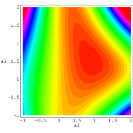
Figure 2: Countour plot of the coefficient $e^{(1)}$ as a function of $\alpha_{2}$ and $\alpha_{3}$ at $\alpha_{1}=1.0$. The colour spectrum goes from violet (higher values) to red (lower values).

Upon this premises, we collect our results in Table 3. It is understood that all the conditions employed define the improvement coefficients up to ${\rm O}(a)\$terms and need to be extrapolated to the continuum limit.

For what concerns the axial current, we obtain the coefficient ${c^{\rm stat(1)}_{\rm\scriptscriptstyle A}}$ from three independent improvement conditions, i.e. at $\theta\in\{0.5,0.75,1.0\}$ and renormalised quark mass $z=Lm_{\rm\scriptscriptstyle R}=0.0$. Having determined ${c^{\rm stat(1)}_{\rm\scriptscriptstyle A}}$, we obtain ${b^{\rm stat(1)}_{\rm\scriptscriptstyle A}}$ from three new independent conditions, i.e at $\theta\in\{0.0,0.5,1.0\}$ and $z=0.24$. Continuum approach is shown in Figs. 4–4.

As for the vector current, we obtain the coefficient ${c^{\rm stat(1)}_{\rm\scriptscriptstyle V}}$ from three different implementations of the axial Ward Identity, corresponding to pairs of $\theta$-angles $(\theta_{1},\theta_{2})\in\{(0.0,0.5),(0.0,1.0),(0.5,1.0)\}$, and the coefficient ${b^{\rm stat(1)}_{\rm\scriptscriptstyle V}}$ from the ratio of a three-point correlator of the static vector current at renormalised quark masses $(z_{1},z_{2})=(0.0,0.24)$ and three values of the $\theta$-angle, viz. $\theta\in\{0.0,0.5,1.0\}$. Convergence to the continuum limit is shown in Figs. 6–6.

In all cases, different definitions lead to a consistent continuum limit. The uncertainty on the final numbers has been estimated as the maximal difference of the continuum extrapolations corresponding to independent definitions. Data fits have been performed according to the asymptotic expansion

$$C\left(\frac{a}{L}\right)=C+A_{1}\left(\frac{a}{L}\right)+B_{1}\left(\frac{a}{L}\right)\log\left(\frac{a}{L}\right)+A_{2}\left(\frac{a}{L}\right)^{2}+B_{2}\left(\frac{a}{L}\right)^{2}\log\left(\frac{a}{L}\right)+\dots$$ (51)

with $C={c^{\rm stat(1)}_{\rm\scriptscriptstyle A}},{b^{\rm stat(1)}_{\rm\scriptscriptstyle A}},{c^{\rm stat(1)}_{\rm\scriptscriptstyle V}},{b^{\rm stat(1)}_{\rm\scriptscriptstyle V}}$.

$[i,j,k]$ $e^{(1)}_{ijk}$ $[0,0,0]$ $\phantom{-}0.168487(1)$ $[1,0,0]$ $-0.222222(1)$ $[1,1,0]$ $-0.041164(1)$ $[1,1,1]$ $-0.015484(1)$ $[2,0,0]$ $\phantom{-}0.111111(1)$ $[2,2,0]$ $\phantom{-}0.023521(1)$ $[2,2,1]$ $-0.002620(1)$ $[2,2,2]$ $\phantom{-}0.019055(1)$ Table 2: Coefficients of the static self-energy at one-loop order of PT.

action ${\rm X}$ $c^{{\rm stat}(1)}_{\rm\scriptscriptstyle X}$ $b^{{\rm stat}(1)}_{\rm\scriptscriptstyle X}$ HYP1 A 00.0029(2) -0.0906(2) HYP1 V -0.0223(6) -0.0212(8) HYP2 A -0.0518(2) -0.142(1) HYP2 V -0.0380(6) -0.0462(8) Table 3: Improvement coefficients of the static-light currents at one-loop order of PT.

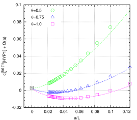
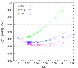
Figure 3: Continuum extrapolation of the improvement coefficient ${c^{\rm stat(1)}_{\rm\scriptscriptstyle A}}$ with HYP1 (left) and HYP2 (right) static discretisation. On each plot, the three curves refer to independent determinations at $\theta=0.5$ (circles), $\theta=0.75$ (triangles) and $\theta=1.0$ (squares).

Figure 4: Continuum extrapolation of the improvement coefficient ${b^{\rm stat(1)}_{\rm\scriptscriptstyle A}}$ with HYP1 (left) and HYP2 (right) static discretisation. On each plot, the three curves refer to independent determinations at $\theta=0.0$ (circles), $\theta=0.5$ (triangles) and $\theta=1.0$ (squares).

Since ${\rm O}(a)\$lattice artefacts depend upon all the details of the calculation, the information given in the previous paragraphs has to be complemented with further technical details, in order to allow for complete reproducibility. In particular, plots reported in Figs. 4–6 refer to a choice of the critical quark mass as obtained from the PCAC relation. Numerical values used have been taken from refs. [20, 21]. Moreover, the determination of ${b^{\rm stat(1)}_{\rm\scriptscriptstyle A}}$ requires the one-loop coefficient $Z_{\rm\scriptscriptstyle A}^{\rm stat(1)}$ of the renormalisation constant of the static axial current as input. The scheme dependence of this coefficient has no effect on the continuum limit of ${b^{\rm stat(1)}_{\rm\scriptscriptstyle A}}$, but it changes its continuum approach. Here, for each single $\theta$-value, we used a definition of $Z_{\rm\scriptscriptstyle A}^{\rm stat(1)}$ from Eq. (4.14) of ref. [11], where the ${\rm O}(a^{2})$ $\theta$-dependent corrections at finite lattice spacing are taken as part of the definition. This allows for a strong cancellation of the ${\rm O}(a)\$lattice artefacts in ${b^{\rm stat(1)}_{\rm\scriptscriptstyle A}}$ and leads to a safe continuum extrapolation. Finally, the particular implementation of the axial Ward Identity needed for ${c^{\rm stat(1)}_{\rm\scriptscriptstyle V}}$, which has been adopted here, refers to a choice of the lattice topology as ${\cal T}=2$, according to the notation of ref. [10].

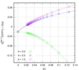
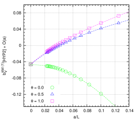
Figure 5: Continuum extrapolation of the improvement coefficient ${c^{\rm stat(1)}_{\rm\scriptscriptstyle V}}$ with HYP1 (left) and HYP2 (right) static discretisation. On each plot, the three curves refer to independent determinations at $(\theta_{1},\theta_{2})=(0.0,0.5)$ (circles), $(\theta_{1},\theta_{2})=(0.0,1.0)$ (triangles) and $(\theta_{1},\theta_{2})=(0.5,1.0)$ (squares).

Figure 6: Continuum extrapolation of the improvement coefficient ${b^{\rm stat(1)}_{\rm\scriptscriptstyle V}}$ with HYP1 (left) and HYP2 (right) static discretisation. On each plot, the three curves refer to independent determinations at $\theta=0.0$ (circles), $\theta=0.5$ (triangles) and $\theta=1.0$ (squares).

Once the improvement coefficients have been determined, one can look at the residual ${\rm O}(a^{2})$ lattice artefacts of the observables from which those coefficients are extracted. As an example, we consider the cutoff effects

$$\delta X^{\rm\scriptscriptstyle I}_{\rm\scriptscriptstyle R}(a/L)=\frac{X^{\rm\scriptscriptstyle I}_{\rm\scriptscriptstyle R}(a/L)}{X^{\rm\scriptscriptstyle I}_{\rm\scriptscriptstyle R}(0)}-1\ ,\qquad X_{\rm\scriptscriptstyle R}^{\rm\scriptscriptstyle I}={Z^{\rm stat}_{\rm\scriptscriptstyle A}}\frac{\,f^{\rm stat}_{\rm\scriptscriptstyle A}+{c^{\rm stat}_{\rm\scriptscriptstyle A}}f^{\rm stat}_{\rm\scriptscriptstyle\delta A}\,}{\sqrt{f_{1}^{\rm stat}}}\ ,$$ (52)

of the ratio $X_{\rm\scriptscriptstyle R}^{\rm\scriptscriptstyle I}$ in the chiral limit. Here we choose to renormalise the static axial current in the “lat” scheme, i.e. with ${Z^{\rm stat}_{\rm\scriptscriptstyle A}}$ having only divergent logarithms without finite parts. Eq. (52) can be expandend in PT,

$$X_{\rm\scriptscriptstyle R}^{\rm\scriptscriptstyle I} =X_{\rm\scriptscriptstyle R}^{\rm\scriptscriptstyle I,(0)}+g_{0}^{2}X_{\rm\scriptscriptstyle R}^{\rm\scriptscriptstyle I,(1)}+{\rm O}(g_{0}^{4})\ ,$$ (53)

$$\delta X_{\rm\scriptscriptstyle R}^{\rm\scriptscriptstyle I} =\delta X_{\rm\scriptscriptstyle R}^{\rm\scriptscriptstyle I,(0)}+g_{0}^{2}\delta X_{\rm\scriptscriptstyle R}^{\rm\scriptscriptstyle I,(1)}+{\rm O}(g_{0}^{4})\ ,$$ (54)

$$\delta X_{\rm\scriptscriptstyle R}^{\rm\scriptscriptstyle I,(0)} =\frac{X_{\rm\scriptscriptstyle R}^{\rm\scriptscriptstyle I,(0)}\left(a/L\right)}{X_{\rm\scriptscriptstyle R}^{\rm\scriptscriptstyle I,(0)}\left(0\right)}-1\ ,$$ (55)

$$\delta X_{\rm\scriptscriptstyle R}^{\rm\scriptscriptstyle I,(1)} =\left[\frac{X_{\rm\scriptscriptstyle R}^{\rm\scriptscriptstyle I,(1)}\left(a/L\right)}{X_{\rm\scriptscriptstyle R}^{\rm\scriptscriptstyle I,(0)}\left(a/L\right)}-\frac{X_{\rm\scriptscriptstyle R}^{\rm\scriptscriptstyle I,(1)}\left(0\right)}{X_{\rm\scriptscriptstyle R}^{\rm\scriptscriptstyle I,(0)}\left(0\right)}\right]\frac{X_{\rm\scriptscriptstyle R}^{\rm\scriptscriptstyle I,(0)}\left(a/L\right)}{X_{\rm\scriptscriptstyle R}^{\rm\scriptscriptstyle I,(0)}\left(0\right)}$$ (56)

We note that $\delta X_{\rm\scriptscriptstyle R}^{\rm\scriptscriptstyle I,(0)}$ does not depend upon the choice of the static regularisation. In order to compare lattice artefacts corresponding to different actions, one has to consider at least the one-loop contribution $\delta X_{\rm\scriptscriptstyle R}^{\rm\scriptscriptstyle I,(1)}$, which is plotted in Fig. 7 for EH and HYP2 at $\theta\in\{0.5,0.75\}$. Remarkably, ${\rm O}(a^{2})$ lattice artefacts are less than 0.1% for both actions. Although in principle the smearing of the gauge link could be responsible for an enhancement of the cutoff effects, we do not observe any sign of this in our observables.

It is also important to stress that the perturbative values collected in Table 3 need not to be in agreement with the findings of refs. [2, 10], where a hybrid technique has been adopted, which mixes one-loop perturbative inputs obtained from the EH or APE discretisations with non-perturbative simulations of HYP static fermions. As an example of this, we consider the case of ${b^{\rm stat}_{\rm\scriptscriptstyle V}}$, for which the mixed procedure gives

$$b_{\rm\scriptscriptstyle V,HYP1}^{{\rm stat}} \ \approx\ \frac{1}{2}-0.014(3)g_{0}^{2}+{\rm O}(g_{0}^{4})\ ,$$ (57)

$$b_{\rm\scriptscriptstyle V,HYP2}^{{\rm stat}} \ \approx\ \frac{1}{2}-0.096(8)g_{0}^{2}+{\rm O}(g_{0}^{4})\ .$$ (58)

As it can be observed, the exact perturbative coefficients are sensibly different from the effective ones, which signals the presence of non-negligible ${\rm O}(g_{0}^{4})$ terms within the latter, quantifiable as the differences among the perturbative and the effective values. The hybrid procedure is such that the differences absorb ${\rm O}(g_{0}^{4})$ terms of both actions used in the improvement condition, for the limited range of the bare coupling ($6.0\leq\beta\leq 6.5$) where this has been implemented. A larger discrepancy between the exact improvement coefficients of the two discretisations at ${\rm O}(g_{0}^{4})$ induces a larger discrepancy between the perturbative coefficients of Table 3 and their effective partners. However, we remark that the impact of these ${\rm O}(g_{0}^{4})$ terms is suppressed when ${b^{\rm stat}_{\rm\scriptscriptstyle V}}$ is multiplied by a reasonably small quark mass $am_{\rm q}$. Similar considerations can be done also for the other improvement coefficients.

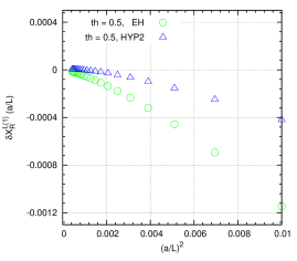
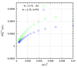
Figure 7: Comparison of the residual ${\rm O}(a^{2})$ lattice artefacts of the improved ratio $X^{\rm\scriptscriptstyle I,(1)}_{\rm\scriptscriptstyle R}$ at one-loop order of PT in the chiral limit, with $\theta=0.5$ (left) and $\theta=0.75$ (right) for the EH (circles) and HYP2 (triangles) actions.

7 Conclusions

In this work, we have studied the ${\rm O}(a)\$improvement of the static axial and vector currents at one-loop order of perturbation theory with hypercubic static and Wilson light quarks. Our methodology for the on-shell ${\rm O}(a)\$improvement is based on the Schrödinger Functional. The calculation is useful in that it allows to quantify the amount of the ${\rm O}(g_{0}^{4})$ terms present in the hybrid perturbative/non-perturbative procedure of refs. [2, 10].

The lack of knowledge of the Feynman rules for the hypercubic static propagator in time-momentum representation has prevented such calculation over the past years. We simply observed that, since the static propagator is a product of temporal hypercubic links, which are not affected by the boundaries of the Schrödinger Functional, the Feynman rules need not to be necessarily derived from scratch, but can be obtained by inverse Fourier transforming in time the ones obtained in full momentum space, the latter being known from the literature [17].

Aside the improvement coefficients, we have found an analytical expression for the static self-energy as a function of the smearing parameters at one-loop order of perturbation theory. This expression has been minimised through an optimal choice of the smearing parameters. We have found that the perturbative minimum is very close to the non-perturbative one, obtained by means of an analogous numerical procedure performed at non-perturbative values of the bare coupling [2, 19]. This is interpreted as a hint of fast perturbative convergence.

Appendix A Derivation of the temporal Feynman rules by direct construction

Owing to the irrelevance of the SU(3) projection at one-loop order of PT, the HYP smearing procedure can be considered as a three-step linear lattice differential operator acting on the gauge fields at subsequent levels. The perturbative expansion of Eqs. (2.1)–(2.1) reads

$$B_{\mu}^{(3)}(x) =(1-\alpha_{1})q_{\mu}(x)+\frac{\alpha_{1}}{3}\sum_{\nu\neq\mu}B_{\mu;\nu}^{(2)}(x)\ +$$

$$+\frac{\alpha_{1}}{6}\sum_{\nu\neq\mu}a^{2}\{\partial^{*}_{\nu}\partial_{\nu}B_{\mu;\nu}^{(2)}(x)-\partial_{\nu}^{*}\partial_{\mu}B_{\nu;\mu}^{(2)}(x)\}\ +{\rm O}(g_{0})\ ,$$ (59)

$$B_{\mu;\nu}^{(2)}(x) =(1-\alpha_{2})q_{\mu}(x)+\frac{\alpha_{2}}{2}\sum_{\rho\neq\mu\nu}B_{\mu;\nu\rho}^{(1)}(x)\ +$$

$$+\frac{\alpha_{1}}{4}\sum_{\rho\neq\mu\nu}a^{2}\{\partial^{*}_{\rho}\partial_{\rho}B_{\mu;\nu\rho}^{(1)}(x)-\partial_{\rho}^{*}\partial_{\mu}B_{\rho;\mu\nu}^{(1)}(x)\}\ +{\rm O}(g_{0})\ ,$$ (60)

$$B_{\mu;\nu\rho}^{(1)}(x) =q_{\mu}(x)+\frac{\alpha_{3}}{2}\sum_{\eta\neq\mu\nu\rho}a^{2}\{\partial^{*}_{\eta}\partial_{\eta}q_{\mu}(x)-\partial_{\eta}^{*}\partial_{\mu}q_{\eta}(x)\}+{\rm O}(g_{0})\ ,$$ (61)

where $\partial_{\mu}$ and $\partial_{\mu}^{*}$ denote respectively the standard forward and backward lattice derivatives.

Since in the SF perturbative calculations are naturally performed in time-momentum representation, the above formulae must be Fourier-transformed along the spatial directions. Before any explicit calculation, it is worth first deciding what is relevant to our aims. To be concrete, we are interested in $\tilde{B}_{0}^{(3)}$. Accordingly, the Lorentz sums in Eq. (A) are purely spatial. The only components of $B_{\mu;\nu}^{(2)}$ to be considered are $B_{0;k}^{(2)}$ and $B_{k;0}^{(2)}$ with $k=1,2,3$. Analogously it can be argued of the following steps. If the notation “$A\leadsto B$” means that $B$ is needed to calculate $A$, then the whole calculation is summarised by

$$B_{0}^{(3)}\ \leadsto\ B_{0;k}^{(2)}\ ,\ B_{k;0}^{(2)}\ ,\qquad\qquad k =1,2,3\ ;$$ (62)

$$B_{0;k}^{(2)}\ \leadsto\ B_{0;k\ell}^{(1)}\ ,\ B_{\ell;0k}^{(1)}\ ,\qquad\qquad k \neq\ell=1,2,3\ ;$$ (63)

$$B_{k;0}^{(2)}\ \leadsto\ B_{k;0\ell}^{(1)}\ ,\ B_{\ell;0k}^{(1)}\ ,\qquad\qquad k \neq\ell=1,2,3\ .$$ (64)

In order to obtain $\tilde{B}_{0}^{(3)}$ we first consider the Fourier transforms of Eqs. (A)–(61) separately. Afterwards, we insert the expression obtained for the first-level smeared gauge fields $\tilde{B}^{(1)}_{\mu;\nu\rho}$ into $\tilde{B}^{(2)}_{\mu;\nu}$ and the latter into $\tilde{B}^{(3)}_{0}$. The Fourier transform of the first-level smeared gauge field is given by

$$\tilde{B}_{0;k\ell}^{(1)}(x_{0};{\mathbf{p}}) =\biggl{\{}1-\frac{\alpha_{3}}{2}\sum_{m\neq k\ell}a^{2}\hat{p}_{m}^{2}\biggr{\}}\tilde{q}_{0}(x_{0};{\mathbf{p}})-i\frac{\alpha_{3}}{2}\sum_{m\neq k\ell}(a\hat{p}_{m})a\partial_{0}\tilde{q}_{m}(x_{0};{\mathbf{p}})\ ,$$ (65)

$$\tilde{B}_{k;0\ell}^{(1)}(x_{0};{\mathbf{p}}) =\biggl{\{}1-\frac{\alpha_{3}}{2}\sum_{m\neq k\ell}a^{2}\hat{p}_{m}^{2}\biggr{\}}\tilde{q}_{k}(x_{0};{\mathbf{p}})+\frac{\alpha_{3}}{2}\sum_{m\neq k\ell}(a\hat{p}_{m})(a\hat{p}_{k})\tilde{q}_{m}(x_{0};{\mathbf{p}})\ ,$$ (66)

$$\tilde{B}_{\ell;0k}^{(1)}(x_{0};{\mathbf{p}}) =\biggl{\{}1-\frac{\alpha_{3}}{2}\sum_{m\neq k\ell}a^{2}\hat{p}_{m}^{2}\biggr{\}}\tilde{q}_{\ell}(x_{0};{\mathbf{p}})+\frac{\alpha_{3}}{2}\sum_{m\neq k\ell}(a\hat{p}_{m})(a\hat{p}_{l})\tilde{q}_{m}(x_{0};{\mathbf{p}})\ ,$$ (67)

where $\hat{p}_{k}\equiv(2/a)\sin(ap_{k}/2)$ denotes a lattice momentum. In particular, it should be remarked that $m\neq k,\ell$, i.e. the sum over $m$ contains just one term. Similarly, one finds

$$\tilde{B}_{0;k}^{(2)}(x_{0};{\mathbf{p}}) =(1-\alpha_{2})\tilde{q}_{0}(x_{0};{\mathbf{p}})+\frac{\alpha_{2}}{4}\sum_{\ell\neq k}(2-a^{2}\hat{p}_{\ell}^{2})\tilde{B}_{0;k\ell}^{(1)}(x_{0};{\mathbf{p}})\ +$$

$$-i\frac{\alpha_{2}}{4}\sum_{\ell\neq k}(a\hat{p}_{\ell})a\partial_{0}\tilde{B}_{\ell;0k}^{(1)}(x_{0};{\mathbf{p}})\ ,$$ (68)

$$\tilde{B}_{k;0}^{(2)}(x_{0};{\mathbf{p}}) =(1-\alpha_{2})\tilde{q}_{k}(x_{0};{\mathbf{p}})+\frac{\alpha_{2}}{4}\sum_{\ell\neq k}(2-a^{2}\hat{p}_{\ell}^{2})\tilde{B}_{k;0\ell}^{(1)}(x_{0};{\mathbf{p}})\ +$$

$$+\frac{\alpha_{2}}{4}\sum_{\ell\neq k}(a\hat{p}_{\ell})(a\hat{p}_{k})\tilde{B}_{\ell;0k}^{(1)}(x_{0};{\mathbf{p}})\ ,$$ (69)

as for the second-level smeared gauge field. Finally,

$$\tilde{B}_{0}^{(3)}(x_{0};{\mathbf{p}}) =(1-\alpha_{1})\tilde{q}_{0}(x_{0};{\mathbf{p}})+\frac{\alpha_{1}}{6}\sum_{k=1}^{3}(2-a^{2}\hat{p}_{k}^{2})\tilde{B}^{(2)}_{0;k}(x_{0};{\mathbf{p}})\ +$$

$$-i\frac{\alpha_{1}}{6}\sum_{k=1}^{3}(a\hat{p}_{k})a\partial_{0}\tilde{B}^{(2)}_{k;0}(x_{0};{\mathbf{p}})\ .$$ (70)

Instead of working out the whole expression alltogether, we observe that the final result is expected to be a linear combination of $\tilde{q}_{0}(x_{0};{\mathbf{p}})$, $\tilde{q}_{k}(x_{0};{\mathbf{p}})$ and $\tilde{q}_{k}(x_{0}+a;{\mathbf{p}})$. Single contributions can be considered separately.

In order to extract the coefficient of $\tilde{q}_{0}(x_{0},{\mathbf{p}})$, we observe that $\tilde{B}_{k;0\ell}^{(1)}$ and $\tilde{B}_{\ell;0k}^{(1)}$ have no temporal gauge field, which appears only in $\tilde{B}_{0;k\ell}^{(1)}$. Accordingly, $\tilde{B}^{(2)}_{k;0}$ is independent of $\tilde{q}_{0}$. Instead, $\tilde{B}^{(2)}_{0;k}$ has such dependence. The coefficient $c_{0}^{(2)}$ multiplying $\tilde{q}_{0}$ in $\tilde{B}^{(2)}_{0;k}$ can be easily isolated, i.e.

$$c_{0}^{(2)}=1-\frac{\alpha_{2}}{4}(1+\alpha_{3})\sum_{\ell\neq k}a^{2}\hat{p}_{\ell}^{2}+\frac{\alpha_{2}\alpha_{3}}{4}\prod_{\ell\neq k}a^{2}\hat{p}_{\ell}^{2}\ .$$ (71)

Analogously, the coefficient $c_{0}^{(3)}$ multiplying $\tilde{q}_{0}$ in $\tilde{B}_{0}^{(3)}$ can be isolated upon replacing $\tilde{B}_{0;k}^{(2)}$ with its explicit value. Some algebra leads to

$$c_{0}^{(3)}=(1-\alpha_{1})+\frac{\alpha_{1}}{6}\sum_{k}(2-a^{2}\hat{p}_{k}^{2})c_{0}^{(2)}=f_{00}(p)\ .$$ (72)

A similar procedure allows to extract the spatial contributions to $\tilde{B}_{0}^{(3)}(x_{0};{\mathbf{p}})$.

Appendix B Spatial parallel transporter

In this appendix we report the Feynman rules for the spatial HYP link in time-momentum representation. We follow sect. 4 and base our derivation on the inverse Fourier transform of the Feynman rules in momentum space, first obtained in ref. [17]. We start from Eq. (36),

$$\tilde{B}_{k}^{(3)}(p)=f_{k0}(p)\tilde{q}_{0}(p)+\!\sum_{\eta\neq 0,k}\!f_{k\eta}(p)\tilde{q}_{\eta}(p)+f_{kk}(p)\tilde{q}_{k}(p)+{\rm O}(g_{0})\,.$$ (73)

Contributions on the right hand side are worked out separately. Some algebra leads to the expressions

$$\tilde{B}_{k}^{(3;1)}(x_{0};{\mathbf{p}}) \equiv\frac{1}{L}\sum_{p_{0}}{\rm e}^{ip_{0}x_{0}}f_{k0}(p)\tilde{q}_{0}(p)=$$

$$=-i\frac{\alpha_{1}}{6}(a\hat{p}_{k})\Omega_{k0}({\mathbf{p}})a\partial_{0}^{*}\tilde{q}_{0}(x_{0};{\mathbf{p}})\ ,$$ (74)

$$\tilde{B}_{k}^{(3;2)}(x_{0};{\mathbf{p}}) \equiv\frac{1}{L}\sum_{p_{0}}{\rm e}^{ip_{0}x_{0}}\sum_{\eta\neq 0,k}f_{k\eta}(p)\tilde{q}_{\eta}(p)=$$

$$=(a\hat{p}_{k})\sum_{\eta\neq 0,k}\left[\Delta_{k\eta}^{\rm(s)}({\mathbf{p}})+\Delta_{k\eta}^{\rm(t)}({\mathbf{p}})a^{2}\partial_{0}^{*}\partial_{0}\right]\tilde{q}_{\eta}(x_{0};{\mathbf{p}})\ ,$$ (75)

$$\tilde{B}_{k}^{(3;3)}(x_{0};{\mathbf{p}}) \equiv\frac{1}{L}\sum_{p_{0}}{\rm e}^{ip_{0}x_{0}}f_{kk}(p)\tilde{q}_{k}(p)=$$

$$=\biggl{\{}1+\frac{\alpha_{1}}{6}\Omega_{k0}({\mathbf{p}})a^{2}\partial_{0}^{*}\partial_{0}-\biggr{.}$$

$$-\biggl{.}\phantom{\int}\sum_{\eta\neq 0,k}(a\hat{p}_{\eta})\left[\Delta_{k\eta}^{\rm(s)}({\mathbf{p}})+\Delta_{k\eta}^{\rm(t)}({\mathbf{p}})a^{2}\partial_{0}^{*}\partial_{0}\right]\biggr{\}}\tilde{q}_{k}(x_{0};{\mathbf{p}})\ ,$$ (76)

where we have introduced the symbols

$$\Delta_{k\eta}^{\rm(s)}({\mathbf{p}}) =\frac{\alpha_{1}}{6}(a\hat{p}_{\eta})\left[1+\alpha_{2}(1+\alpha_{3})-\frac{\alpha_{2}}{4}(1+2\alpha_{3})(a^{2}\hat{p}^{2}_{\ell\neq k,\eta})\right]\ ,$$ (77)

$$\Delta_{k\eta}^{\rm(t)}({\mathbf{p}}) =\frac{\alpha_{1}}{6}(a\hat{p}_{\eta})\left[\frac{\alpha_{2}}{4}(1+2\alpha_{3})-\frac{\alpha_{2}\alpha_{3}}{4}(a^{2}\hat{p}_{\ell\neq k,\eta}^{2})\right]\ .$$ (78)

Eqs.(B)-(B) can be written in the compact form

$$\tilde{B}_{k}^{(3)}(x_{0};{\mathbf{p}})=\sum_{i=0}^{7}V_{k;i}({\mathbf{p}})\tilde{q}_{\mu(i)}(x_{0}+as(i);{\mathbf{p}})\ ,$$ (79)

where the vertex $V_{k;i}({\mathbf{p}})$ and the auxiliary indices $\mu$, $s$ are collected in Table 4.

$i$	$\mu(i)$	$s(i)$	$V_{k;i}({\mathbf{p}})$
0	0	-0	$-i\frac{\alpha_{1}}{6}a\hat{p}_{k}\Omega_{k0}({\mathbf{p}})$
1	0	-1	$\phantom{-}i\frac{\alpha_{1}}{6}a\hat{p}_{k}\Omega_{k0}({\mathbf{p}})$
2	k	-0	$1-\frac{\alpha_{1}}{3}\Omega_{k0}({\mathbf{p}})\,+\,\sum_{\eta\neq 0,k}a\hat{p}_{\eta}\,[2\Delta_{k\eta}^{\rm(t)}({\mathbf{p}})-\Delta_{k\eta}^{\rm(s)}({\mathbf{p}})]$
3	k	-1	$\frac{\alpha_{1}}{6}\Omega_{k0}({\mathbf{p}})-\sum_{\eta\neq 0,k}a\hat{p}_{\eta}\Delta_{k\eta}^{\rm(t)}({\mathbf{p}})$
4	k	-1	$\frac{\alpha_{1}}{6}\Omega_{k0}({\mathbf{p}})-\sum_{\eta\neq 0,k}a\hat{p}_{\eta}\Delta_{k\eta}^{\rm(t)}({\mathbf{p}})$
5	$\eta;0k$	-0	$a\hat{p}_{k}[\Delta_{k\eta}^{(s)}({\mathbf{p}})-2\Delta_{k\eta}^{\rm(t)}({\mathbf{p}})]$
6	$\eta;0k$	-1	$a\hat{p}_{k}\Delta_{k\eta}^{\rm(t)}({\mathbf{p}})$
7	$\eta;0k$	-1	$a\hat{p}_{k}\Delta_{k\eta}^{\rm(t)}({\mathbf{p}})$

Table 4: Feynman rules of the spatial HYP link in time-momentum representation. The symbol $\eta;0k$ denotes a sum over $\eta\neq 0,k$.

Appendix C Derivation of Eq. (48)

To conclude, we detail the calculation of the static self-energy and provide a derivation of Eq. (48). We consider the boundary-to-boundary correlator $f_{1}^{\rm stat}$, defined in ref. [11] via

$$f_{1}^{\rm stat}=-\frac{a^{12}}{2L^{6}}\sum_{{\mathbf{u}}{\mathbf{v}}{\mathbf{y}}{\mathbf{z}}}\langle\overline{\zeta}^{\prime}({\mathbf{u}})\gamma_{5}\zeta^{\prime}_{\rm h}({\mathbf{v}})\overline{\zeta}_{\rm h}({\mathbf{y}})\gamma_{5}\zeta({\mathbf{z}})\rangle\ .$$ (80)

Expanding $f_{1}^{\rm stat}$ at one-loop order of PT allows to write the coefficient $e^{(1)}$, see Eq. (47), in terms of the Feynman diagrams of Fig. 1, i.e.

$$e^{(1)} =-\lim_{a/L\to 0}\frac{4}{3}\frac{a}{L^{4}}\sum_{\mathbf{p}}a^{2}\sum_{u_{0}=a}^{T}\sum_{v_{0}=a}^{u_{0}}b(u_{0},v_{0})\sum_{i,j=0}^{6}\delta_{\mu(i)\mu(j)}V_{0;i}({\mathbf{p}})V_{0;j}(-{\mathbf{p}})\ \times$$

$$\times d_{\mu(i)\mu(j)}(u_{0}-a+as(i),v_{0}-a+as(j);{\mathbf{p}})\ =$$

$$\equiv-\lim_{a/L\to 0}\frac{4}{3}\frac{1}{L^{3}}\sum_{\mathbf{p}}a^{2}\sum_{u_{0}=a}^{T}\sum_{v_{0}=a}^{u_{0}}b(u_{0},v_{0}){\cal V}(u_{0},v_{0},{\mathbf{p}})\ ,$$ (81)

where $d_{\mu\nu}(x_{0},y_{0},{\mathbf{p}})$ denotes the gluon propagator in time-momentum representation, cf. ref. [13] for a definition. The weight-coefficient $b(u_{0},v_{0})$ is given by

$$b(u_{0},v_{0})=\left\{\begin{array}[]{cl}1/2&\quad u_{0}=v_{0}\ ,\\[5.16663pt] 1&\quad{\rm otherwise}\ ,\end{array}\right.$$ (82)

and the interaction blob

$${\cal V}(u_{0},v_{0},{\mathbf{p}})=\sum_{i,j=0}^{6}\delta_{\mu(i)\mu(j)}V_{0;i}({\mathbf{p}})V_{0;j}(-{\mathbf{p}})d_{\mu(i)\mu(j)}(u_{0}-a+as(i),v_{0}-a+as(j);{\mathbf{p}})$$ (83)

denotes a HYP gluon propagating on the lattice from time $u_{0}$ to time $v_{0}$ with spatial momentum ${\mathbf{p}}$. The above expression can be simplified by using spatial rotational invariance, i.e. $d_{11}=d_{22}=d_{33}$ and $d_{ij}=0$ if $i\neq j$. Accordingly, the vertex reads

$${\cal V}(u_{0},v_{0},{\mathbf{p}}) =|V_{0;0}({\mathbf{p}})|^{2}d_{00}(u_{0}-a,v_{0}-a;{\mathbf{p}})\ +$$

$$+\left[|V_{0;1}({\mathbf{p}})|^{2}+|V_{0;2}({\mathbf{p}})|^{2}+|V_{0;3}({\mathbf{p}})|^{2}\right]\ \times$$

$$\times\left[d_{kk}(u_{0}-a,v_{0}-a;{\mathbf{p}})+d_{kk}(u_{0},v_{0};{\mathbf{p}})\right.\ -$$

$$-\left.d_{kk}(u_{0},v_{0}-a;{\mathbf{p}})-d_{kk}(u_{0}-a,v_{0};{\mathbf{p}})\right]\ .$$ (84)

From Eq. (C), we conclude that the HYP vertex $V_{0;j}({\mathbf{p}})$ enters the coefficient $e^{(1)}$ only in the rotationally symmetric combinations

$$h^{\rm(t)}({\mathbf{p}}) =|V_{0;0}({\mathbf{p}})|^{2}\ ,$$

$$h^{\rm(s)}({\mathbf{p}}) =|V_{0;1}({\mathbf{p}})|^{2}+|V_{0;2}({\mathbf{p}})|^{2}+|V_{0;3}({\mathbf{p}})|^{2}\ .$$ (85)

These quantities are multivariate polynomials of the HYP smearing parameters, i.e.

$$h^{\rm(t,s)}({\mathbf{p}})=\sum_{k_{1}k_{2}k_{3}=0}^{2}w^{\rm(t,s)}_{k_{1}k_{2}k_{3}}({\mathbf{p}})\alpha_{1}^{k_{1}}\alpha_{2}^{k_{2}}\alpha_{3}^{k_{3}}\ ,\qquad w^{\rm(t,s)}_{k_{1}k_{2}k_{3}}=\frac{1}{k_{1}!k_{2}!k_{3}!}\frac{\partial^{k_{1}+k_{2}+k_{3}}h^{\rm(t,s)}}{\partial\alpha_{1}^{k_{1}}\partial\alpha_{2}^{k_{2}}\partial\alpha_{3}^{k_{3}}}\ .$$ (86)

The coefficients $w^{\rm(t,s)}_{k_{1}k_{2}k_{3}}$ have been written according to the generic Taylor expansion in several variables. They can be algebraically evaluated; the non-vanishing ones are reported in sect. C.1 in units of the lattice spacing. Spatial rotational invariance is evident.

Upon inserting Eq. (86) into Eq. (C) and Eq. (C) into Eq. (C), the final result represented by Eq. (48) is obtained with coefficients

$$e^{(1)}_{k_{1}k_{2}k_{3}}=\lim_{a/L\to 0}\frac{4}{3}\frac{a}{L^{4}}\sum_{\mathbf{p}}a^{2}\sum_{u_{0}=a}^{T}\sum_{v_{0}=a}^{u_{0}}b(u_{0},v_{0})\ \times$$

$$\times\left\{w^{\rm(t)}_{k_{1}k_{2}k_{3}}({\mathbf{p}})d_{00}(u_{0}-a,v_{0}-a;{\mathbf{p}})\ +\right\}$$

$$+w^{\rm(s)}_{k_{1}k_{2}k_{3}}({\mathbf{p}})\left[d_{kk}(u_{0}-a,v_{0}-a;{\mathbf{p}})+d_{kk}(u_{0},v_{0};{\mathbf{p}})\ -\right.$$

$$\left.\left.-d_{kk}(u_{0},v_{0}-a;{\mathbf{p}})-d_{kk}(u_{0}-a,v_{0};{\mathbf{p}})\right]\right\}\ .$$ (87)

C.1 Coefficients $w_{\rm t,s}^{k_{1}k_{2}k_{3}}$

$$w^{\rm(t)}_{{000}} =1\ ,$$ (88)

$$w^{\rm(t)}_{{100}} =-\frac{1}{3}\,({{\hat{p}_{1}}}^{2}+{{\hat{p}_{2}}}^{2}+{{\hat{p}_{3}}}^{2})\ ,$$ (89)

$$w^{\rm(t)}_{{110}} =-\frac{1}{3}\,({{\hat{p}_{1}}}^{2}+{{\hat{p}_{2}}}^{2}+{{\hat{p}_{3}}}^{2})+\frac{1}{6}\,({{\hat{p}_{1}}}^{2}{{\hat{p}_{2}}}^{2}+{{\hat{p}_{1}}}^{2}{{\hat{p}_{3}}}^{2}+{{\hat{p}_{2}}}^{2}{{\hat{p}_{3}}}^{2})\ ,$$ (90)

$$w^{\rm(t)}_{{111}} =-\frac{1}{3}\,({{\hat{p}_{1}}}^{2}+{{\hat{p}_{2}}}^{2}+{{\hat{p}_{3}}}^{2})+\frac{1}{3}\,({{\hat{p}_{1}}}^{2}{{\hat{p}_{2}}}^{2}+{{\hat{p}_{1}}}^{2}{{\hat{p}_{3}}}^{2}+{{\hat{p}_{2}}}^{2}{{\hat{p}_{3}}}^{2})-\frac{1}{4}\,{{\hat{p}_{1}}}^{2}{{\hat{p}_{2}}}^{2}{{\hat{p}_{3}}}^{2}\ ,$$ (91)

$$w^{\rm(t)}_{{200}} =\frac{1}{36}\,({{\hat{p}_{1}}}^{4}+{{\hat{p}_{2}}}^{4}+{{\hat{p}_{3}}}^{4})+\frac{1}{18}\,({{\hat{p}_{1}}}^{2}{{\hat{p}_{2}}}^{2}+{{\hat{p}_{1}}}^{2}{{\hat{p}_{3}}}^{2}+{{\hat{p}_{2}}}^{2}{{\hat{p}_{3}}}^{2})\ ,$$ (92)

$$w^{\rm(t)}_{{210}} =\frac{1}{18}({{\hat{p}_{1}}}^{4}+{{\hat{p}_{2}}}^{4}+{{\hat{p}_{3}}}^{4})+\frac{1}{9}\,({{\hat{p}_{1}}}^{2}{{\hat{p}_{2}}}^{2}+{{\hat{p}_{1}}}^{2}{{\hat{p}_{3}}}^{2}+{{\hat{p}_{2}}}^{2}{{\hat{p}_{3}}}^{2})\ -$$

$$-\frac{1}{36}\,({{\hat{p}_{1}}}^{4}{{\hat{p}_{2}}}^{2}+{{\hat{p}_{1}}}^{4}{{\hat{p}_{3}}}^{2}+{{\hat{p}_{2}}}^{4}{{\hat{p}_{1}}}^{2}+{{\hat{p}_{2}}}^{4}{{\hat{p}_{3}}}^{2}+{{\hat{p}_{3}}}^{4}{{\hat{p}_{1}}}^{2}+{{\hat{p}_{3}}}^{4}{{\hat{p}_{2}}}^{2})-\frac{1}{12}\,{{\hat{p}_{1}}}^{2}{{\hat{p}_{2}}}^{2}{{\hat{p}_{3}}}^{2}\ ,$$ (93)

$$w^{\rm(t)}_{{211}} =\frac{1}{18}\,({{\hat{p}_{1}}}^{4}+{{\hat{p}_{2}}}^{4}+{{\hat{p}_{3}}}^{4})+\frac{1}{9}\,({{\hat{p}_{1}}}^{2}{{\hat{p}_{2}}}^{2}+{{\hat{p}_{1}}}^{2}{{\hat{p}_{3}}}^{2}+{{\hat{p}_{2}}}^{2}{{\hat{p}_{3}}}^{2})\ -$$

$$-\frac{1}{18}\,({{\hat{p}_{1}}}^{4}{{\hat{p}_{2}}}^{2}+{{\hat{p}_{1}}}^{4}{{\hat{p}_{3}}}^{2}+{{\hat{p}_{2}}}^{4}{{\hat{p}_{1}}}^{2}+{{\hat{p}_{2}}}^{4}{{\hat{p}_{3}}}^{2}+{{\hat{p}_{3}}}^{4}{{\hat{p}_{1}}}^{2}+{{\hat{p}_{3}}}^{4}{{\hat{p}_{2}}}^{2})-\frac{1}{6}\,{{\hat{p}_{1}}}^{2}{{\hat{p}_{2}}}^{2}{{\hat{p}_{3}}}^{2}\ +$$

$$+\frac{1}{24}\,({{\hat{p}_{1}}}^{4}{{\hat{p}_{2}}}^{2}{{\hat{p}_{3}}}^{2}+{{\hat{p}_{2}}}^{4}{{\hat{p}_{1}}}^{2}{{\hat{p}_{3}}}^{2}+{{\hat{p}_{3}}}^{4}{{\hat{p}_{1}}}^{2}{{\hat{p}_{2}}}^{2})\ ,$$ (94)

$$w^{\rm(t)}_{{220}} =\frac{1}{36}\,({{\hat{p}_{1}}}^{4}+{{\hat{p}_{2}}}^{4}+{{\hat{p}_{3}}}^{4})+\frac{1}{18}(\,{{\hat{p}_{1}}}^{2}{{\hat{p}_{2}}}^{2}+{{\hat{p}_{1}}}^{2}{{\hat{p}_{3}}}^{2}+{{\hat{p}_{2}}}^{2}{{\hat{p}_{3}}}^{2})-\frac{1}{12}\,{{\hat{p}_{1}}}^{2}{{\hat{p}_{2}}}^{2}{{\hat{p}_{3}}}^{2}\ -$$

$$-\frac{1}{36}\,({{\hat{p}_{1}}}^{4}{{\hat{p}_{2}}}^{2}+{{\hat{p}_{1}}}^{4}{{\hat{p}_{3}}}^{2}+{{\hat{p}_{2}}}^{4}{{\hat{p}_{1}}}^{2}+\,{{\hat{p}_{2}}}^{4}{{\hat{p}_{3}}}^{2}+{{\hat{p}_{3}}}^{4}{{\hat{p}_{1}}}^{2}+{{\hat{p}_{3}}}^{4}{{\hat{p}_{2}}}^{2})\ +$$

$$+\frac{1}{72}\,({{\hat{p}_{1}}}^{4}{{\hat{p}_{2}}}^{2}{{\hat{p}_{3}}}^{2}+{{\hat{p}_{2}}}^{4}{{\hat{p}_{1}}}^{2}{{\hat{p}_{3}}}^{2}+{{\hat{p}_{3}}}^{4}{{\hat{p}_{1}}}^{2}{{\hat{p}_{2}}}^{2})+\frac{1}{144}\,({{\hat{p}_{1}}}^{4}{{\hat{p}_{2}}}^{4}+{{\hat{p}_{1}}}^{4}{{\hat{p}_{3}}}^{4}+{{\hat{p}_{2}}}^{4}{{\hat{p}_{3}}}^{4})\ ,$$ (95)

$$w^{\rm(t)}_{221} =\frac{1}{18}\,({\hat{p}_{1}}^{4}+{\hat{p}_{2}}^{4}+{\hat{p}_{3}}^{4})+\frac{1}{9}\,({\hat{p}_{1}}^{2}{\hat{p}_{2}}^{2}+{\hat{p}_{1}}^{2}{\hat{p}_{3}}^{2}+{\hat{p}_{2}}^{2}{\hat{p}_{3}}^{2})\ -$$

$$-\frac{1}{12}\,({\hat{p}_{1}}^{4}{\hat{p}_{2}}^{2}+{\hat{p}_{1}}^{4}{\hat{p}_{3}}^{2}+{\hat{p}_{2}}^{4}{\hat{p}_{1}}^{2}+{\hat{p}_{2}}^{4}{\hat{p}_{3}}^{2}+{\hat{p}_{3}}^{4}{\hat{p}_{1}}^{2}+{\hat{p}_{3}}^{4}{\hat{p}_{2}}^{2})-\frac{1}{4}\,{\hat{p}_{1}}^{2}{\hat{p}_{2}}^{2}{\hat{p}_{3}}^{2}\ +$$

$$+\frac{1}{36}\,({\hat{p}_{1}}^{4}{\hat{p}_{2}}^{4}+{\hat{p}_{1}}^{4}{\hat{p}_{3}}^{4}+{\hat{p}_{2}}^{4}{\hat{p}_{3}}^{4})+\frac{7}{72}\,({\hat{p}_{1}}^{4}{\hat{p}_{2}}^{2}{\hat{p}_{3}}^{2}+{\hat{p}_{2}}^{4}{\hat{p}_{1}}^{2}{\hat{p}_{3}}^{2}+{\hat{p}_{3}}^{4}{\hat{p}_{1}}^{2}{\hat{p}_{2}}^{2})\ -$$

$$-\frac{1}{48}\,({\hat{p}_{1}}^{4}{\hat{p}_{2}}^{4}{\hat{p}_{3}}^{2}+{\hat{p}_{1}}^{4}{\hat{p}_{3}}^{4}{\hat{p}_{2}}^{2}+{\hat{p}_{2}}^{4}{\hat{p}_{3}}^{4}{\hat{p}_{1}}^{2})\ ,$$ (96)

$$w^{\rm(t)}_{222} =\frac{1}{36}\,({\hat{p}_{1}}^{4}+{\hat{p}_{2}}^{4}+{\hat{p}_{3}}^{4})+\frac{1}{18}\,({\hat{p}_{1}}^{2}{\hat{p}_{2}}^{2}+{\hat{p}_{1}}^{2}{\hat{p}_{3}}^{2}+{\hat{p}_{2}}^{2}{\hat{p}_{3}}^{2})\ -$$

$$-\frac{1}{6}\,{\hat{p}_{1}}^{2}{\hat{p}_{2}}^{2}{\hat{p}_{3}}^{2}-\frac{1}{18}\,({\hat{p}_{1}}^{4}{\hat{p}_{2}}^{2}+{\hat{p}_{1}}^{4}{\hat{p}_{3}}^{2}+{\hat{p}_{2}}^{4}{\hat{p}_{1}}^{2}+{\hat{p}_{2}}^{4}{\hat{p}_{3}}^{2}+{\hat{p}_{3}}^{4}{\hat{p}_{1}}^{2}+{\hat{p}_{3}}^{4}{\hat{p}_{2}}^{2})\ +$$

$$+\frac{1}{36}\,({\hat{p}_{1}}^{4}{\hat{p}_{2}}^{4}+{\hat{p}_{1}}^{4}{\hat{p}_{3}}^{4}+{\hat{p}_{2}}^{4}{\hat{p}_{3}}^{4})+\frac{7}{72}\,({\hat{p}_{1}}^{4}{\hat{p}_{2}}^{2}{\hat{p}_{3}}^{2}+{\hat{p}_{2}}^{4}{\hat{p}_{1}}^{2}{\hat{p}_{3}}^{2}+{\hat{p}_{3}}^{4}{\hat{p}_{1}}^{2}{\hat{p}_{2}}^{2})\ -$$

$$-\frac{1}{24}\,({\hat{p}_{1}}^{4}{\hat{p}_{2}}^{4}{\hat{p}_{3}}^{2}+{\hat{p}_{1}}^{4}{\hat{p}_{3}}^{4}{\hat{p}_{2}}^{2}+{\hat{p}_{2}}^{4}{\hat{p}_{3}}^{4}{\hat{p}_{1}}^{2})\ +\frac{1}{64}\,{\hat{p}_{1}}^{4}{\hat{p}_{2}}^{4}{\hat{p}_{3}}^{4}\ .$$ (97)

$$w^{\rm(s)}_{200} =\frac{1}{18}\,({\hat{p}_{1}}^{2}+{\hat{p}_{2}}^{2}+{\hat{p}_{3}}^{2})\ ,$$ (98)

$$w^{\rm(s)}_{210} =\frac{1}{9}\,({\hat{p}_{1}}^{2}+{\hat{p}_{2}}^{2}+{\hat{p}_{3}}^{2})-\frac{1}{18}\,({\hat{p}_{1}}^{2}{\hat{p}_{2}}^{2}+{\hat{p}_{1}}^{2}{\hat{p}_{3}}^{2}+{\hat{p}_{2}}^{2}{\hat{p}_{3}}^{2})\ ,$$ (99)

$$w^{\rm(s)}_{211} =\frac{1}{9}\,({\hat{p}_{1}}^{2}+{\hat{p}_{2}}^{2}+{\hat{p}_{3}}^{2})-\frac{1}{9}(\,{\hat{p}_{1}}^{2}{\hat{p}_{2}}^{2}+{\hat{p}_{1}}^{2}{\hat{p}_{3}}^{2}+{\hat{p}_{2}}^{2}{\hat{p}_{3}}^{2})+\frac{1}{12}\,{\hat{p}_{1}}^{2}{\hat{p}_{2}}^{2}{\hat{p}_{3}}^{2}\ ,$$ (100)

$$w^{\rm(s)}_{220} =\frac{1}{9}\,({\hat{p}_{1}}^{2}+{\hat{p}_{2}}^{2}+{\hat{p}_{3}}^{2})-\frac{1}{9}\,({\hat{p}_{1}}^{2}{\hat{p}_{2}}^{2}+{\hat{p}_{1}}^{2}{\hat{p}_{3}}^{2}+{\hat{p}_{2}}^{2}{\hat{p}_{3}}^{2})\ +$$

$$+\frac{1}{144}\,({\hat{p}_{1}}^{4}{\hat{p}_{2}}^{2}+{\hat{p}_{1}}^{4}{\hat{p}_{3}}^{2}+{\hat{p}_{2}}^{4}{\hat{p}_{1}}^{2}+{\hat{p}_{2}}^{4}{\hat{p}_{3}}^{2}+{\hat{p}_{3}}^{4}{\hat{p}_{1}}^{2}+{\hat{p}_{3}}^{4}{\hat{p}_{2}}^{2})+\frac{1}{24}\,{\hat{p}_{1}}^{2}{\hat{p}_{2}}^{2}{\hat{p}_{3}}^{2}\ ,$$ (101)

$$w^{\rm(s)}_{221} =\frac{2}{9}\,({\hat{p}_{1}}^{2}+{\hat{p}_{2}}^{2}+{\hat{p}_{3}}^{2})-\frac{1}{3}\,({\hat{p}_{1}}^{2}{\hat{p}_{2}}^{2}+{\hat{p}_{1}}^{2}{\hat{p}_{3}}^{2}+{\hat{p}_{2}}^{2}{\hat{p}_{3}}^{2})\ +$$

$$+\frac{1}{36}\,({\hat{p}_{1}}^{4}{\hat{p}_{2}}^{2}+{\hat{p}_{1}}^{4}{\hat{p}_{3}}^{2}+{\hat{p}_{2}}^{4}{\hat{p}_{1}}^{2}+{\hat{p}_{2}}^{4}{\hat{p}_{3}}^{2}+{\hat{p}_{3}}^{4}{\hat{p}_{1}}^{2}+{\hat{p}_{3}}^{4}{\hat{p}_{2}}^{2})+\frac{1}{3}\,{\hat{p}_{1}}^{2}{\hat{p}_{2}}^{2}{\hat{p}_{3}}^{2}\ -$$

$$-\frac{1}{36}\,({\hat{p}_{1}}^{4}{\hat{p}_{2}}^{2}{\hat{p}_{3}}^{2}+{\hat{p}_{2}}^{4}{\hat{p}_{1}}^{2}{\hat{p}_{3}}^{2}+{\hat{p}_{3}}^{4}{\hat{p}_{1}}^{2}{\hat{p}_{2}}^{2})\ ,$$ (102)

$$w^{\rm(s)}_{222} =\frac{2}{9}\,({\hat{p}_{1}}^{2}+{\hat{p}_{2}}^{2}+{\hat{p}_{3}}^{2})-\frac{4}{9}\,({\hat{p}_{1}}^{2}{\hat{p}_{2}}^{2}+{\hat{p}_{1}}^{2}{\hat{p}_{3}}^{2}+{\hat{p}_{2}}^{2}{\hat{p}_{3}}^{2})\ +$$

$$+\frac{1}{18}\,({\hat{p}_{1}}^{4}{\hat{p}_{2}}^{2}+{\hat{p}_{1}}^{4}{\hat{p}_{3}}^{2}+{\hat{p}_{2}}^{4}{\hat{p}_{1}}^{2}+{\hat{p}_{2}}^{4}{\hat{p}_{3}}^{2}+{\hat{p}_{3}}^{4}{\hat{p}_{1}}^{2}+{\hat{p}_{3}}^{4}{\hat{p}_{2}}^{2})+\frac{2}{3}\,{\hat{p}_{1}}^{2}{\hat{p}_{2}}^{2}{\hat{p}_{3}}^{2}\ +$$

$$-\frac{1}{9}\,({\hat{p}_{1}}^{4}{\hat{p}_{2}}^{2}{\hat{p}_{3}}^{2}+{\hat{p}_{2}}^{4}{\hat{p}_{1}}^{2}{\hat{p}_{3}}^{2}+{\hat{p}_{3}}^{4}{\hat{p}_{1}}^{2}{\hat{p}_{2}}^{2})+\frac{1}{72}\,({\hat{p}_{1}}^{4}{\hat{p}_{2}}^{4}{\hat{p}_{3}}^{2}+{\hat{p}_{1}}^{4}{\hat{p}_{3}}^{4}{\hat{p}_{2}}^{2}+{\hat{p}_{2}}^{4}{\hat{p}_{3}}^{4}{\hat{p}_{1}}^{2})\ .$$ (103)

References

[1]
A. Hasenfratz and F. Knechtli,
Phys. Rev. D 64 (2001) 034504,
[arXiv:hep-lat/0103029].
[2]
M. Della Morte, A. Shindler and R. Sommer,
JHEP 0508 (2005) 051,
[arXiv:hep-lat/0506008].
[3]
E. Eichten and B. R. Hill,
Phys. Lett. B 234 (1990) 511.
[4]
M. Della Morte, N. Garron, M. Papinutto and R. Sommer,
JHEP 0701 (2007) 007,
[arXiv:hep-ph/0609294].
[5]
D. Guazzini, H. B. Meyer and R. Sommer,
JHEP 0710 (2007) 081,
arXiv:0705.1809 [hep-lat].
[6]
M. Della Morte et al.,
arXiv:0710.2201 [hep-lat].
[7]
F. Palombi, M. Papinutto, C. Pena and H. Wittig,
JHEP 0709 (2007) 062,
arXiv:0706.4153 [hep-lat].
[8]
F. Palombi, M. Papinutto, C. Pena and H. Wittig,
PoS LAT2007 (2007) 366,
arXiv:0710.2863 [hep-lat].
[9]
P. Dimopoulos et al.,
arXiv:0712.2429 [hep-lat].
[10]
F. Palombi,
JHEP 01 (2008) 021,
arXiv:0706.2460 [hep-lat].
[11]
M. Kurth and R. Sommer,
Nucl. Phys. B 597, 488 (2001),
[arXiv:hep-lat/0007002].
[12]
M. Luscher, R. Narayanan, P. Weisz and U. Wolff,
Nucl. Phys. B 384 (1992) 168,
[arXiv:hep-lat/9207009].
[13]
M. Luscher and P. Weisz,
Nucl. Phys. B 479 (1996) 429,
[arXiv:hep-lat/9606016].
[14]
R. Sommer,
[arXiv:hep-lat/0611020].
[15]
W. j. Lee,
Phys. Rev. D 66 (2002) 114504,
[arXiv:hep-lat/0208032].
[16]
J. A. M. Vermaseren,
[arXiv:math-ph/0010025].
[17]
A. Hasenfratz, R. Hoffmann and F. Knechtli,
Nucl. Phys. Proc. Suppl. 106 (2002) 418,
[arXiv:hep-lat/0110168].
[18]
A. Hasenfratz, R. Hoffmann and S. Schaefer,
JHEP 0705 (2007) 029,
[arXiv:hep-lat/0702028].
[19]
R. Sommer, private communications.
[20]
F. Palombi, C. Pena and S. Sint,
JHEP 0603 (2006) 089,
[arXiv:hep-lat/0505003].
[21]
F. Palombi, M. Papinutto, C. Pena and H. Wittig,
JHEP 0608 (2006) 017,
[arXiv:hep-lat/0604014].