Higher representations on the lattice: perturbative studies

Abstract:

We present analytical results to guide numerical simulations with Wilson fermions in higher representations of the colour group. The ratio of $\Lambda$ parameters, the additive renormalization of the fermion mass, and the renormalization of fermion bilinears are computed in perturbation theory, including cactus resummation. We recall the chiral Lagrangian for the different patterns of symmetry breaking that can take place with fermions in higher representations, and discuss the possibility of an Aoki phase as the fermion mass is reduced at finite lattice spacing.

1 Introduction

The nonperturbative dynamics of asymptotically free gauge theories with matter fields transforming according to higher dimensional representations of the underlying gauge group is a topic of current research interest. Physics beyond the Standard Model (BSM) offers a new arena for the use of these theories, which are expected to develop a nonperturbative infrared fixed point for a very low number of flavors [1, 2]. Because they minimize the tension with the electroweak precision constraints, some of these theories are excellent candidates for the dynamical breaking of the electroweak symmetry of walking technicolor type, which were first introduced in Refs. [3, 4, 5, 6, 7, 8]. Since the number of flavors needed to get near the conformal fixed point is small, the associated models have been termed minimal walking technicolor [1, 2, 9]. By walking one refers to the fact that the running coupling decreases much more slowly with the reference energy scale than in the case of QCD–like theories. Yet, another interesting physical application of the study of the phase diagram of strongly coupled theories is to provide the theoretical landscape underlying the unparticle physics world [10, 11]. The theory landscape was provided in Ref. [12] where it was shown that the fraction of asymptotically free gauge theories developing an infrared fixed point is quite large. Studying their phase diagram is a fundamental step if these theories aspire to become realistic candidates for BSM physics. Insight into the phase diagram of such theories has been recently provided by a proposed all-order beta function for any number of colours and for any representation [13]. Moreover, in the limit of a large number of colours, the planar orientifold planar equivalence relates theories with fermions in higher representations to supersymmetric theories [14]. It provides interesting predictions that deserve nonperturbative investigations [15, 16]. The necessity to study the large-$N$ limit makes these theories more expensive to study numerically. Finally, understanding the strong dynamics that governs the low–energy behaviour of such theories is an interesting problem per se.

Lattice is a privileged tool for exploring the nonperturbative dynamics of strongly interacting theories, but Monte Carlo simulations of these theories can capture the interesting dynamical features only if the full fermion determinant is taken into account in the Boltzmann weight used for generating gauge configurations. So far only limited experience has been gathered from numerical simulations with dynamical fermions beyond QCD [17, 18]. In the light of recent algorithmic progresses in simulating quantum field theories with dynamical fermions [19, 20, 21, 22, 23, 24], numerical studies with fermions in higher–dimensional representations are now a realistic target (see Ref. [18] for early work in this direction). As a preliminary work, which provides guidance for large–scale simulations, we present here an investigation of the space of bare couplings by analytical tools, such as perturbation theory and chiral Lagrangians.

Perturbative results are useful to understand the behaviour of the lattice theory as the continuum limit is approached: on one hand they provide a connection between the lattice results and their continuum counterparts; on the other hand they offer some quantitative support in choosing the bare parameters in the early stages of numerical simulations. Precision studies in QCD have shown sizable discrepancies between perturbative and nonperturbative computations at the values of the bare parameters that are currently accessible. Assessing the accuracy of perturbation theory for theories with fermions in higher–dimensional representations is beyond the scope of this paper and will be deferred to future publications. Instead we shall supplement perturbative calculations with sensible assumptions, that we discuss below, in order to dictate the choice of the values of the bare parameters for first numerical investigations.

In this work perturbation theory is used to determine the dependence of the lattice spacing on the bare lattice coupling, the ratio of lambda parameters $\Lambda_{\overline{\mathrm{MS}}}/\Lambda_{\mathrm{lat}}$, the critical value of the bare mass $m_{c}$ and critical hopping parameter $\kappa_{c}$, and the renormalization constants for fermionic bilinears. The gauge action considered is the simple plaquette action, and the fermion action is the unimproved Wilson action. This simple choice provides a concrete example for performing the perturbative calculations, and matches the existing, and forthcoming numerical simulations. Four specific examples of lattice theories with Wilson fermions are compared below. Results for quenched QCD (QCD0), and for QCD with two flavours of dynamical fermions (QCD2) are known both in perturbation theory, and from non–perturbative computations. They are briefly summarized in this work in order to set the framework for our computations, and to assess the accuracy of perturbation theory. We then present the generalization of the perturbative calculations to arbitrary representations, and analyze in detail their implications for two theories that are good candidates for BSM phenomenology, namely the SU(3) gauge theory with $n_{f}=2$ flavours in the two–index symmetric representation (T1), and the SU(2) gauge theory with two flavours in the two–index symmetric representation (T2).

The chiral Lagrangian describing the dynamics of the light Goldstone bosons is analyzed in order to clarify the structure of the phase diagram that is likely to be revealed by numerical simulations for small quark masses. We discuss in particular the theories with fermions in higher representations introduced above. Note that the same approach can be readily applied to other theories, like e.g. gauge theories with fermions in the two–index antisymmetric representations, that are interesting for numerical tests of the planar orientifold equivalence. Even though we do not discuss these theories explicitly here, our conclusions can be specialized in a straightforward manner.

The paper is organized as follows. In Sect. 2 we discuss the perturbative results describing asymptotic scaling, we compute the ratio of $\Lambda$ parameters, and discuss the approach of the continuum limit. Sect. 3 reports some useful results at one–loop in perturbation theory. We first consider the renormalization of the bare mass for Wilson fermions; the critical value of the hopping parameter $\kappa_{c}$ is computed both up to two loops, and using the so–called cactus dressing to resum a particular class of tadpole diagrams [25]. Similarly we present results for the renormalization constants for fermion bilinears. Finally in Sect. 4 we discuss the form of the chiral Lagrangian that describes the low–energy dynamics in theories with fermions in arbitrary representation and the possible phase structure as the quark mass is lowered at finite lattice spacing.

Numerical simulations of the theories with fermions in higher representations are deferred to further publications.

2 Scaling

2.1 Ratio of $\Lambda$ parameters

The $\beta$ function encodes the dependence of the lattice spacing $a$ on the bare coupling constant $g_{0}$. In mass–independent renormalization schemes, the lattice spacing is uniquely determined by the bare coupling, according to the renormalization group equation:

$$\beta_{\mathrm{lat}}(g_{0})=-a\left.\frac{\partial g_{0}}{\partial a}\right|_{g_{R}~{}\mathrm{fixed}},$$ (1)

where the subscript $\mathrm{lat}$ refers to the lattice scheme which is being considered here.

For a generic gauge theory, with gauge group SU($N$) and $n_{f}$ fermions in a given representation $R$ of the colour group, the two–loop computation in perturbation theory yields the familiar expression:

$$\beta_{\mathrm{lat}}(g_{0}) = -\beta_{0}g_{0}^{3}-\beta_{1}g_{0}^{5}+O(g_{0}^{7})$$ (2)

$$\beta_{0} = \frac{1}{(4\pi)^{2}}\left[\frac{11}{3}C_{2}(A)-\frac{4}{3}T_{R}n_{f}\right]$$ (3)

$$\beta_{1} = \frac{1}{(4\pi)^{4}}\left[\frac{34}{3}C_{2}(A)^{2}-\frac{20}{3}C_{2}(A)T_{R}n_{f}-4C_{2}(R)T_{R}n_{f}\right],$$ (4)

where $T_{R}$ yields the normalization of the generators, and $C_{2}(R)$ is the quadratic Casimir, both in the representation $R$. Factors of $C_{2}(A)$, the quadratic Casimir in the adjoint representation, arise because of gluon loops, and do not change as the fermionic representation is varied. Note that the first two coefficients of the $\beta$ function are universal and depend neither on the regularization nor on the renormalization scheme. For $N=3$ and fermions in the fundamental representation, the expressions above reduce to the usual values of $\beta_{0},\beta_{1}$. Tables for the group–theoretical factors for the representations considered in this work are reported in App. A.

The asymptotic behaviour of $a(g_{0})$ is obtained by integrating Eq. (1), and the scale $\Lambda_{\mathrm{lat}}$ is the integration constant that appears in this procedure. Following the notation in Ref. [26], we write:

$$a(g_{0})\Lambda_{\mathrm{lat}} = \exp\left[-\int^{g_{0}}\frac{dg^{\prime}}{\beta_{\mathrm{lat}}(g^{\prime})}\right]$$ (5)

$$= \exp\left[-1/(2\beta_{0}g_{0}^{2})\right]\left(\beta_{0}g_{0}^{2}\right)^{-\beta_{1}/(2\beta_{0}^{2})}\left[1+O(g_{0}^{2})\right].$$

The ratio of $\Lambda$–parameters defined in different renormalization schemes is obtained from the one–loop relation between the coupling constants [27, 28, 29, 26]. In particular the running coupling in the $\overline{\mathrm{MS}}$ scheme is related to the lattice bare coupling via:

$$g_{\overline{\mathrm{MS}}}(\mu)=\left\{1+\sum_{l=1}^{\infty}{\mathcal{Z}}^{(l)}(\mu a,\lambda_{0})g_{0}^{2l}\right\}^{-1/2}g_{0},$$ (6)

where $\lambda_{0}$ is the bare gauge–fixing parameter in the lattice formulation. This relation can be obtained e.g. using the background field technique [30, 31, 32]. The first coefficient ${\mathcal{Z}}^{(1)}(\mu a,\lambda_{0})$ for matter fields in the fundamental representation can be found in the literature, see e.g. Ref. [29, 26]. It has the generic form:

$$\left.{\mathcal{Z}}^{(1)}(\mu a,\lambda_{0})\right|_{\lambda_{0}=1}=\beta_{0}\log(a^{2}\mu^{2})+l_{0},$$ (7)

and the ratio of $\Lambda$–parameters is obtained from the coefficients in Eq. (7) as:

$$\Lambda_{\mathrm{lat}}/\Lambda_{\overline{\mathrm{MS}}}=\exp\left[l_{0}/(2\beta_{0})\right].$$ (8)

Having already written the coefficient $\beta_{0}$ for a generic representation in Eq. (3), the expression for the finite part of the one–loop contribution in Eq. (6), $l_{0}$, is the only ingredient needed in order to convert the $\Lambda$–parameter. The coefficient $l_{0}$ is obtained by inspecting the one–loop diagrams that contribute to Eq. (7). The group–theoretical factors need to be changed in order to take into account the new fermionic representation, while the numerical factors that arise from the integration over the lattice momenta remain unchanged. For a generic representation $R$, we obtain:

$$l_{0} = \frac{1}{(8\pi^{2})}\left[-2\pi^{2}\;C_{2}(F)-3.54958342046\;C_{2}(A)+\right.$$ (9)

$$\left.+1.057389936\;T_{R}n_{f}\right],$$

where the only dependence on the fermionic representation is encoded in the last term in the sum on the RHS of Eq. (9). Explicit values for some representations of interest are summarized in Tab. 1. The well–known values for the quenched SU(2) and SU(3) theories, and for QCD with two flavours of fundamental fermions are reported in order to show explicitly the differences in the perturbative coefficients as we introduce matter in higher representations. As a non–trivial check, we can specialize Eq. (9) to the case of ${\mathcal{N}}=1$ SYM, which corresponds to $n_{f}=1/2$ flavour of fermions in the adjoint representation. Using the group–theoretical factors reported in Tab. 2 in Appendix A, our expression reproduces Eq. (24) in Ref. [33].

Representation	$\beta_{0}$	$\beta_{1}$	$l_{0}$
SU(2), $n_{f}=0$	0.0464389	0.00181793	-0.277412
SU(3), $n_{f}=0$	0.0696583	0.00409035	-0.468201
SU(2), $n_{f}=2$, fund	0.0612149	0.00307445	-0.454809
SU(3), $n_{f}=2$, fund	0.0612149	0.00307445	-0.454809
SU(3), $n_{f}=2$, 2S	0.0274412	-0.00259323	-0.401241
SU(2), $n_{f}=2$, 2S	0.0126651	-0.00160406	-0.223844

Table 1: Perturbative coefficients appearing in one-loop perturbative computations.

The ratios of $\Lambda$–parameters are easily obtained from the values in Tab. 1. The coefficients in the first lines of the table reproduce the known results:

$$\left.\Lambda_{\overline{\mathrm{MS}}}/\Lambda_{\mathrm{lat}}\right|_{\mathrm{SU(2)},n_{f}=0} = 19.82,$$ (10)

$$\left.\Lambda_{\overline{\mathrm{MS}}}/\Lambda_{\mathrm{lat}}\right|_{\mathrm{SU(3)},n_{f}=0} = 28.81,$$ (11)

$$\left.\Lambda_{\overline{\mathrm{MS}}}/\Lambda_{\mathrm{lat}}\right|_{\mathrm{SU(3)},n_{f}=2,\mathrm{fund}} = 41.05,$$ (12)

see e.g. Refs. [28, 29, 26]. The last two lines yield the new results for the higher representations that we want to consider in this work:

$$\left.\Lambda_{\overline{\mathrm{MS}}}/\Lambda_{\mathrm{lat}}\right|_{\mathrm{SU(3)},n_{f}=2,2S} = 1469.59$$ (13)

$$\left.\Lambda_{\overline{\mathrm{MS}}}/\Lambda_{\mathrm{lat}}\right|_{\mathrm{SU(2)},n_{f}=2,2S} = 6884.36.$$ (14)

Values for other representations can be easily deduced from the formulae above. Including two flavours of fermions in higher representations induces large variations in the ratios of $\Lambda$ parameters. This is at odds with the results for fermions in the fundamental representation, where adding the effect of fermion loops yields a much smaller variation of the ratio. However the large values obtained for fermions in two–index representations can be understood by rewriting the ratio $\beta_{0}/2l_{0}$ in a way which makes the $1/N$ scaling explicit:

$$\frac{l_{0}}{2\beta_{0}}\simeq-3.65978\cdot\frac{1-0.0787969T_{R}\frac{n_{f}}{N}-0.735484\frac{1}{N^{2}}}{1-\frac{4}{11}T_{R}\frac{n_{f}}{N}}.$$ (15)

In Eq. (15) we can easily recognize the contributions $O(n_{f}/N)$ from fermion loops, and the contributions from the non–planar gluonic diagrams of $O(1/N^{2})$. For fermions in the fundamental representation $T_{R}=1/2$, and therefore the fermion determinant yields corrections that are suppressed by $n_{f}/N$. For fermions in 2–index representations, the normalization of the generators is such that $T_{R}\sim O(N)$, and hence the contribution from the fermion determinant is of the same order of the gluon contribution, both in the numerator and the denominator, and therefore large variations are found with respect to the pure gauge theory.

2.2 Perturbative and nonperturbative scaling

The perturbative results obtained in the previous subsection can be used to sketch the scaling of the lattice spacing for theories in higher representations, being well aware of the limitations of perturbation theory. The nonperturbative scaling of the lattice spacing has been carefully studied for QCD, both in the quenched approximation, and for the theory with dynamical quarks in the fundamental representation. For the latter theories, the accuracy of perturbative estimates can be assessed by comparing numerical and analytical results. As we shall see below, perturbation theory in QCD does not yield an accurate description of the scaling of physical quantities. Therefore, any result obtained in this framework is bound to be approximate and should be used mostly as a guide for forthcoming numerical simulations.

In order to relate more easily to the notation used in numerical simulations, let us introduce the lattice coupling $\beta=2N/g_{0}^{2}$. We will henceforth use $\beta$ to indicate the bare lattice coupling, unless explicitly stated. The asymptotic scaling formula reported in the previous subsection yields the value of the lattice spacing in physical units as a function of $\beta$:

$$\frac{a^{-1}(\beta)}{\Lambda_{\overline{\mathrm{MS}}}}=\left(\frac{\Lambda_{\mathrm{lat}}}{\Lambda_{\overline{\mathrm{MS}}}}\right)\exp\left[\frac{\beta}{4N\beta_{0}}\right]\left(2N\beta_{0}/\beta\right)^{\beta_{1}/(2\beta_{0}^{2})}\left[1+O(1/\beta)\right].$$ (16)

Having computed the ratio of $\Lambda$ parameters, the only input that is required is the value of $\Lambda_{\overline{\mathrm{MS}}}$.

For the SU(3) pure gauge theory, Fig. 1 displays the prediction for the lattice spacing $a$ in physical units [fm], computed from two–loop perturbation theory using the input from Ref. [34, 35]; the curve is compared to the interpolation of the nonperturbative data presented in [36]. The error band in the figure is simply the error that is obtained from propagating the error in the determination of $\Lambda_{\overline{\mathrm{MS}}}$ to the value of $a(\beta)$. As shown by the plot, the perturbative prediction in bare perturbation theory underestimates the actual lattice spacing by 30–50% at the values of $\beta$ between 5.8 and 6.2, where most simulations have been performed so far. The two computations agree at large values of $\beta$, as expected when the continuum limit is approached.

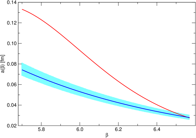
Figure 1: Comparison of the lattice scaling in physical units predicted from perturbation theory with the nonperturbative results obtained from numerical simulations. The theory is pure gauge SU(3). The blue (respectively red) curve represents the perturbative (resp. nonperturbative) estimate of the lattice spacing in fm as a function of the lattice bare coupling $\beta$. The error on the perturbative estimate comes from the error in the determination of $\Lambda_{\overline{\mathrm{MS}}}$. The red curve is an interpolation of the nonpertubative determination of the lattice spacing.

For the SU(3) theory with two flavours of Wilson fermions, the perturbative prediction is obtained using the $\Lambda$ parameter computed in Ref. [37, 38]; it can be compared to the value of the lattice spacing recently computed for two values of $\beta$ in Ref. [39]. Again, in the range that is accessible to current simulations, the perturbative estimate is smaller by approximately 30%–40%. Such large deviations between lattice bare perturbation theory and nonperturbative results are very well-known to lattice QCD practitioners [40]. They are reported here in order to have a concise summary of the results in QCD, before moving into new territories.

Figure 2 shows the perturbative estimate for the value of the dimensionless quantity $a(\beta)\Lambda_{\overline{\mathrm{MS}}}$ for QCD with $n_{f}=0,2$ in the same range of $\beta$; for the values of $\beta$ used in current simulations, one can see that $1/(a\Lambda_{\overline{\mathrm{MS}}})\approx 20$. Given that the hadron masses in QCD turn out to be of the order of $\Lambda_{\overline{\mathrm{MS}}}$, the value of $1/(a\Lambda_{\overline{\mathrm{MS}}})$ is such that lattice artefacts are small, while sufficiently large physical volumes can be reached on lattices that have 20–30 points in each direction. Lattice simulations for theories beyond QCD need to identify a similar regime in order to avoid large lattice artefacts and/or large finite volume effects.

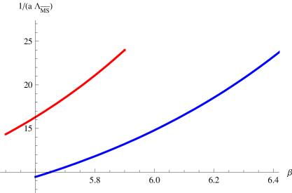
Figure 2: The perturbative result for the dimensionless quantity $a(\beta)\Lambda_{\overline{\mathrm{MS}}}$ as a function of $\beta$ for pure gauge SU(3) (blue line), and SU(3) with $n_{f}=2$ flavours of Wilson fermions (red line).

Perturbative results can be used for the theories with fermions in higher representations in order to arrive at an educated guess for the value of $\Lambda_{\overline{\mathrm{MS}}}a(\beta)$ from perturbative scaling, provided a few hypotheses are made in order to identify the relevant energy scales. As already mentioned in the introduction, a near–conformal behaviour is expected in the theories T1 and T2. The dependence of the coupling on the lattice spacing in these theories is characterized by two different regimes. At high energies the theories are asymptotically free, and therefore we expect the usual logarithmic running of the renormalized coupling. However, as the energy scale is decreased, it should reach a value, which we denote $\Lambda_{\mathrm{w}}$, where the coupling starts to “walk”, i.e. where the coupling is only weakly dependent on the cutoff. The walking behaviour should extend for several orders of magnitude, until a lower scale $\Lambda_{\mathrm{IR}}$ where the coupling starts running again. Phenomenologically relevant models would favour a ratio $\Lambda_{\mathrm{w}}/\Lambda_{\mathrm{IR}}\geq 10^{3}$ [2]. However, it should be noted that the running of the coupling constant is scheme dependent, and therefore this ratio should only be taken as an indicative value.

The perturbative values of $\Lambda_{\overline{\mathrm{MS}}}a(\beta)$ as a function of $\beta$ are reported in Fig. 3 for the theories T1 and T2. If we assume that $\Lambda_{\overline{\mathrm{MS}}}\sim\Lambda_{\mathrm{IR}}$, and if we further require that $\Lambda_{\mathrm{w}}a(\beta)\approx 0.1$, then numerical simulations of phenomenologically relevant models would require $\Lambda_{\overline{\mathrm{MS}}}a(\beta)\leq 10^{-5}$. The range of $\beta$ in the figure is chosen to yield values of $\Lambda_{\overline{\mathrm{MS}}}a(\beta)$ that saturate the inequality above; if the ratio between the typical hadron masses turn out to be large in units of $\Lambda_{\overline{\mathrm{MS}}}$, so that $m_{\mathrm{had}}a\simeq 1$, then higher values of $\beta$ would be needed in order to keep both lattice artefacts and finite volume effects under control. More quantitative information can only be obtained from numerical simulations.

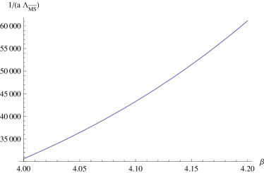
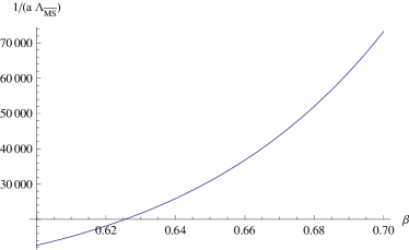
Figure 3: The lattice spacing in unit of $\Lambda_{\overline{\mathrm{MS}}}$ as a function of $\beta$ for the theory T1 (left), and T2 (right).

As already seen above, in numerical simulations of QCD nonperturbative scaling does deviate from the two–loop predictions by up to 50%. We should therefore take these perturbative results with a grain of salt.

It is worthwhile to emphasize that, while we have expressed everything in units of $\Lambda_{\overline{\mathrm{MS}}}$, the absolute value of the scale for these new theories is not known a priori, and can only be determined by computing some physical dimensionful quantity. An obvious candidate would be the decay constant of the technipion in the chiral limit, which is related to the Higgs vev and can be estimated to be $F\approx 250~{}\mathrm{GeV}$.

Nonperturbative results that could highlight the near–conformal behaviour can be obtained by Monte Carlo renormalization group methods [41, 42]. However these methods require to vary the lattice cutoff over a large interval, while simultaneously keeping the finite–size errors under control. If the physical scales of interest are well separated, lattice simulations require a very fine resolution, i.e. a large number of lattice points, that may not be accessible with present–day computing resources.

The finite–volume schemes introduced in Ref. [43] provide an elegant solution to this problem; the renormalization scale is identified with the inverse of the linear lattice size, and the evolution of the renormalized coupling is computed in steps, changing the scale $\mu$ by factors of 2 in each step. The variation of the coupling is summarized in the step–scaling function, which yields a precise determination of the nonperturbative beta function. Recent results for the theory with $n_{f}=12$ fermions in the fundamental representation show that this is a promising way to study the problem [44].

3 Perturbative renormalization

In order to perform numerical simulations, preliminary estimates of the critical mass and of the renormalization of fermion bilinears are needed. This section summarizes some useful computations at one and two loops in perturbation theory for fermions in generic representations, that can be used to guide preliminary lattice studies. We will consider here the theory defined on the lattice, with Wilson action for the fermions, and simple plaquette action for the gauge fields. In the gauge action, the link variables are always SU($N$) matrices in the fundamental representation, while in the fermionic part of the action, the covariant derivatives are defined through the link variables in the generic representation. Feynman rules for perturbative calculations are easily generalized.

Simulating Wilson fermions, the bare mass in the Lagrangian undergoes an additive renormalization, so that the chiral limit is reached for a critical value $m_{c}$ which needs to be determined nonperturbatively. Again perturbation theory is useful to get some guidance on the initial choice of parameters before embarking in actual simulations.

Following the notation in Ref. [45], we write the perturbative expansion of the one–particle irreducible two point function at zero momentum as:

$$m_{c}(g_{0})=g_{0}^{2}\Sigma^{(1)}+g_{0}^{4}\Sigma^{(2)}+\ldots$$ (17)

At one loop, the usual tadpole and sunset diagrams give rise to two contributions, $c_{1}^{(1)}$ and $c_{2}^{(1)}$, respectively; for a generic fermionic representation $R$, these yield:

$$\Sigma^{(1)}=2C_{2}(R)\left[c_{1}^{(1)}+c_{2}^{(1)}\right].$$ (18)

At this order in perturbation theory, the additive renormalization of the mass is simply proportional to the quadratic Casimir of the fermionic representation, while the proportionality constant $c_{1}^{(1)}+c_{2}^{(1)}$ is independent of the representation. We can therefore use the value in Ref. [45]:

$$\left[c_{1}^{(1)}+c_{2}^{(1)}\right]=-0.162857058711(2).$$ (19)

At two loops we need to inspect the structure of the diagrams listed in Fig. 2 of Ref. [45], and modify the group theoretical factors to take into account the fact that the generators appearing in the vertices involving both fermions and gluons are in a generic representation, whereas generators inside 3- and 4-gluon vertices are still in the fundamental representation. For our present purposes, the result of Ref. [45] (Eq. (9) therein) for $\Sigma^{(2)}$ can be recast in the form:

$$\Sigma^{(2)} = C_{2}(F)\,N\,d_{1}+C_{2}(F)\,n_{f}\,d_{2}+C_{2}(F)^{2}(d_{3}+d_{4}),$$ (20)

$$d_{1} = -0.001940(6)\qquad d_{2}=0.00237236(16)$$ (21)

$$d_{3} = -0.081429(8)\qquad d_{4}=0.01516325(12)$$ (22)

($C_{2}(F)$ is the quadratic Casimir operator in the fundamental representation). In the above, contributions proportional to $C_{2}(F)^{2}$ have been separated into $d_{3}$ (arising solely from the two diagrams with a tadpole made out of the 4-gluon vertex) and $d_{4}$ (coming from the remaining diagrams). The extension to an arbitrary representation $R$ is now immediate:

$$\Sigma^{(2)} = C_{2}(R)\,N\,d_{1}+2C_{2}(R)\,T_{R}\,n_{f}\,d_{2}+C_{2}(R)\,C_{2}(F)\,d_{3}+C_{2}(R)^{2}d_{4}\,,$$ (23)

where the quantities $d_{i}$ are left unchanged.

The prediction from perturbation theory can be improved by resumming a specific infinite class of gauge invariant tadpole diagrams. This method is known under the name of cactus dressing [25], and it has been shown to provide improved estimates for various quantities of interest, bringing them closer to nonperturbative results. Unlike other approaches for improving perturbation theory, such as Refs. [46, 40], this approach does not rely on any Monte Carlo data as input, and it is therefore ideally suited for an exploratory study, such as the present one. Cactus resummation for the one-loop result of the critical mass simply amounts to dividing the result by a factor $\tilde{c}_{0}$ (denoted $(1-w(g_{0}))$ in Ref. [25]), which is independent of the fermion representation (since it arises from an all-order resummation of gluon diagrams), but depends on $N$ and on the bare coupling constant $g_{0}$. The factor $\tilde{c}_{0}$ is the solution of the following equation:

$$u\,e^{-u(N{-}1)/(2N)}\,\left[\frac{N{-}1}{N}\,L^{1}_{N{-}1}(u)+2L^{2}_{N{-}2}(u)\right]=\frac{g_{0}^{2}\,(N^{2}{-}1)}{4},\qquad\tilde{c}_{0}\equiv\frac{g_{0}^{2}}{4u}$$ (24)

($L^{\alpha}_{\beta}\,$ are Laguerre polynomials). For $N=2$ and $N=3$, Eq. (24) simplifies to:

$$\begin{array}[]{lcl}\tilde{c}_{0}=e^{\displaystyle-g_{0}^{2}/(16\,\tilde{c}_{0})}\,\left(1-\frac{\displaystyle g_{0}^{2}}{\displaystyle 24\,\tilde{c}_{0}}\right),&&(N=2)\\ \tilde{c}_{0}=e^{\displaystyle-g_{0}^{2}/(12\,\tilde{c}_{0})}\,\left(1-\frac{\displaystyle g_{0}^{2}}{\displaystyle 8\,\tilde{c}_{0}}+\frac{\displaystyle g_{0}^{4}}{\displaystyle 384\,\tilde{c}_{0}^{2}}\right),&&(N=3).\end{array}$$ (25)

Figure 4 presents $\tilde{c}_{0}$ [47] as a function of $g_{0}^{2}$, for $N=2$ and $N=3$. The range of $g_{0}^{2}$ values, for which a solution exists, extends from $g_{0}^{2}=0$ (where $\tilde{c}_{0}=1$) up to $16/\sqrt{9e}\simeq 3.23$ ($N=2$) and $1.558$ ($N=3$); this covers the whole region of physical interest.

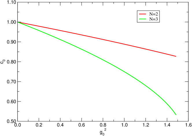
Figure 4: $\tilde{c}_{0}$ as a function of $g_{0}^{2}$ for $N{=}2$ (red line) and $N{=}3$ (green line).

The one–loop resummed result thus simply yields:

$$m_{c}=g_{0}^{2}2C_{2}(R)\left[c_{1}^{(1)}+c_{2}^{(1)}\right]/\tilde{c}_{0}\,,$$ (26)

where $[c_{1}^{(1)}+c_{2}^{(1)}]$ is given in Eq. (19) and $\tilde{c}_{0}$ may be read off Fig. 4.

In actual numerical simulations, the hopping parameter $\kappa$ is used instead of the bare mass $m_{0}$. Based on the studies in Ref. [45], we decide to use the one–loop resummed result as our estimate of the location of the massless theory in the space of bare parameters. The critical value of the hopping parameter is given by: $\kappa_{c}=1/(2m_{c}+8)$, where $m_{c}$ is as in Eq. (26).

In order to compute the decay constant of pseudoscalar mesons, the renormalization of the axial current $Z_{A}$ is needed. While a nonperturbative determination of the renormalization constant is desirable, for the first exploratory studies we shall again rely on perturbation theory to determine $Z_{A}$. The accuracy of perturbation theory can be estimated by comparing the results for QCD, where both a perturbative and a nonperturbative computations are available.

The perturbative renormalization for the axial current with Wilson fermions was originally computed in Ref. [48] – see also Ref. [49] for a useful collection of results for the numerical integrals that appear in lattice calculations. The computation of the renormalization constant for fermion bilinears requires the computation of the vertex functions, and of the fermion wave–function renormalization. For both quantities the Feynman diagrams that appear at one loop depend on the quadratic Casimir of the fermion representation. They are therefore readily generalized to an arbitrary representation, e.g.

$$Z_{V} = 1-\frac{g_{0}^{2}}{16\pi^{2}}C_{2}(R)20.62,$$ (27)

$$Z_{A} = 1-\frac{g_{0}^{2}}{16\pi^{2}}C_{2}(R)15.7,$$ (28)

where the numerical factor is determined by numerical integrals that do not depend on the fermion representation. Using the values for $C_{2}(R)$ in the appendix, the values of $Z_{A}$ and $Z_{V}$ can be easily computed for a generic representation.

The one-loop perturbative results for $Z_{V},\ Z_{A}$ can also be improved via cactus dressing; such an improvement has been known to work rather well with fermions in the fundamental representation [50]. To this effect, all that is required is a substitution of $g_{0}^{2}$ by $g_{0}^{2}/\tilde{c}_{0}$ in Eqs. (27,28), where $\tilde{c}_{0}$ is again read off Fig. 4.

4 Generalized Aoki phases

The low–energy dynamics of the pseudo Goldstone particles is determined by the pattern of chiral symmetry breaking. For theories with $n_{f}>1$ and fermions in a complex representation, such pattern is the same as for QCD, and therefore we expect the same Lagrangian to define the dynamics of the effective theory; clearly the low–energy constants that appear in the Lagrangian do depend on the specific model under study. In this section we discuss the general structure of the chiral Lagrangian for fermions in arbitrary representations, and the possible phases of the theories discretized on the lattice.

4.1 $\mathop{\rm SU}(2)\times\mathop{\rm SU}(2)\rightarrow\mathop{\rm SU}(2)$

For the theory T1 that we have been considering in this work, we have two flavours in a complex representation of the gauge group and therefore the usual $\mathrm{SU}(2)\times\mathop{\rm SU}(2)$ chiral Lagrangian is expected to determine the dynamics in the low–energy theory. Following the notation used in Ref. [51], and including the symmetry breaking terms, yields the Lagrangian:

$${\mathcal{L}}=\frac{F^{2}}{4}\mathrm{Tr}\left(\partial^{\mu}\Sigma^{\dagger}\partial_{\mu}\Sigma\right)+\frac{c_{1}}{4}\mathrm{Tr}\left(\Sigma+\Sigma^{\dagger}\right)-\frac{c_{2}}{16}\left\{\mathrm{Tr}\left(\Sigma+\Sigma^{\dagger}\right)\right\}^{2}.$$ (29)

The pion decay constant in technicolour theories is related to the vacum expectation value of the (composite) Higgs field, which yields $F\approx 250~{}\mathrm{GeV}$. Lattice artefacts for Wilson fermions enter in the coefficients of the symmetry breaking terms:

$$c_{1}\sim\Lambda^{3}\left(m+a\Lambda^{2}\right),~{}~{}~{}~{}~{}c_{2}\sim\Lambda^{2}\left(m^{2}+ma\Lambda^{2}+a^{2}\Lambda^{4}\right),$$ (30)

where $\Lambda$ is again the hadronic scale for the theory under consideration. The pattern of symmetry breaking depends on the coefficients $c_{1}$ and $c_{2}$. Since these coefficients depend on the PCAC mass $m$ and the lattice spacing $a$, the phase diagram can be mapped into the plane of the bare parameters $m_{0},g_{0}$, used in lattice simulations.

The analysis in Ref. [51] remains unchanged; for the theory with two flavours the field $\Sigma$ can be parametrized as:

$$\Sigma=A+i{\mathbf{B}}\cdot{\mathbf{\sigma}},~{}~{}~{}~{}~{}A^{2}+{\mathbf{B}}^{2}=1,$$ (31)

and the potential becomes:

$$-c_{1}A+c_{2}A^{2},$$ (32)

so that the minimum of the potential $\Sigma_{0}=A_{0}+i{\mathbf{B}}_{0}\cdot{\mathbf{\sigma}}$ can develop a non–trivial ${\mathbf{B}}_{0}$ only if $|A_{0}|<1$. For $c_{2}>0$ a region of width $\sim\left(a\Lambda\right)^{3}$ may exist, where the minimum of the potential leads to an Aoki phase. Hence the approach to the chiral limit in theories with two Wilson fermions in any complex representation is similar to the one observed in QCD: as the quark mass is reduced at fixed lattice spacing, flavour symmetry is broken and two massless Goldstone bosons appear. The actual values of $c_{1}$ and $c_{2}$ depend on the dynamics of the theory under study, and need to be estimated for the cases of interest. Nevertheless, in all cases, the chiral limit is entangled with the continuum limit, and the quark mass cannot be lowered to arbitrarily small masses at fixed lattice spacing.

4.2 $\mathop{\rm SU}(4)\rightarrow\mathop{\rm SO}(4)$

In considering theories in arbitrary representations, different patterns of chiral symmetry breaking may occur. The symmetry breaking patterns and the effective theories describing the low–energy dynamics in these cases have been studied e.g. in Refs. [52, 53, 54, 9]. Using this effective theory framework, we discuss the possibility of having an Aoki phase in one case that arises in phenomenologically interesting theories, namely the breaking pattern SU(4)$\to$SO(4).

This symmetry breaking pattern appears for two Dirac fermions in the adjoint representation of the gauge group, see e.g. the theory T2 discussed above. Denoting by $\Sigma$ the Goldstone matrix, the relevant effective potential for the study of the Aoki phase is:

$$V=-\frac{c_{1}}{4}{\rm Tr}\left[\Sigma+\Sigma^{\dagger}\right]+\frac{c_{2}}{16}\left\{\mathrm{Tr}\left(\Sigma+\Sigma^{\dagger}\right)\right\}^{2}.$$ (33)

Here $\Sigma$ transforms linearly under the global symmetry group $\mathrm{SU}(4)$, i.e.

$$\Sigma\rightarrow g\Sigma g^{T}\quad{\rm with}\quad g\in\mathrm{SU}(4)\ ,$$ (34)

and

$$\Sigma=\Sigma_{0}\,\exp(i\sum_{a}^{9}\frac{{\pi}^{a}}{f_{\pi}}X^{a})\ .$$ (35)

In discussing the possibility of an Aoki phase, we are interested in finding at least one vacuum configuration where the condensate is not proportional to the identity. Indicating with $X^{a}$ and $a=1,\ldots,9$ the generators spanning the $\mathop{\rm SU}(4)/\mathop{\rm SO}(4)$ quotient space [52, 9] (an explicit representation of the matrices $X^{a}$ is reported in the appendix), we look for solutions of the form:

$$\Sigma_{0}=2\sqrt{2}(A_{0}+i\,\sum_{a}^{9}A^{a}X^{a})\ ,$$ (36)

where $A^{a}$ are real coefficients. With this Ansatz, and using the explicit expressions for the generators, the unitarity constraint, i.e. $\Sigma_{0}^{\dagger}\Sigma_{0}={\mathbf{1}}$, implies:

$$A_{0}^{2}+\frac{(A_{1}^{2}+A_{2}^{2}+A_{3}^{2})(A_{3}^{2}+A_{9}^{2}+A_{8}^{2})}{A_{3}^{2}}=1\ .$$ (37)

Substituting the expression for $\Sigma_{0}$ in the potential we find:

$$V=4A_{0}^{2}\,c_{2}-2c_{1}A_{0}\ .$$ (38)

For certain values of the potential coefficients $c_{1},c_{2}$, there exists a minimum for $A_{0}$ smaller than one. For instance, by taking $A_{1}=A_{2}=A_{8}=A_{9}=0$, but a nonzero $A_{3}$, we can satisfy the unitarity constraints and $\mathop{\rm SO}(4)$ breaks spontaneously to $\mathop{\rm{}U}(1)\times\mathop{\rm{}U}(1)$. That this is the correct symmetry of the vacuum can be checked by determining which $\mathop{\rm SO}(4)$ generator commutes with $X^{3}$. We have checked that the $S^{3}$ and $S^{4}$ generators of $\mathop{\rm SO}(4)$ explicitly constructed in Ref. [9] are left unbroken and constitute the generators of $\mathop{\rm{}U}(1)\times\mathop{\rm{}U}(1)$. In this case we would expect the emergence of an Aoki phase with four Goldstone bosons associated to the breaking of $\mathop{\rm SO}(4)$ to $\mathop{\rm{}U}(1)\times\mathop{\rm{}U}(1)$.

4.3 $\mathop{\rm SU}(4)\rightarrow\mathop{\rm Sp}(4)$

This symmetry breaking pattern does appear for fermions in pseudo–real representations. The analysis is similar to the one done before, now using the five (rather than nine) $X$ generators presented in the appendix of Ref. [53]. We seek for a solution using the same Ansatz as in the preceding subsection. The potential evaluated on the Ansatz is identical to the one in Eq. (38). In this case the unitarity constraint for $\Sigma_{0}$ yields the condition:

$$A_{0}^{2}+A_{1}^{2}+A_{2}^{2}+A_{3}^{2}+A_{4}^{2}+A_{5}^{2}=1\ ,$$ (39)

For $A_{0}=1$ one recovers the $\mathop{\rm Sp}(4)$ symmetry. On the other hand a minimum with $A_{0}<1$ implies that the $\mathop{\rm Sp}(4)$ symmetry is spontaneously broken to $\mathop{\rm SO}(4)$. We hence have four broken generators of $\mathop{\rm Sp}(4)$ corresponding to $S^{1},S^{2},S^{9}$ and $S^{10}$ in the appendix of Ref. [53]. Again we find that an Aoki phase is possible, with four massless bosons.

4.4 Eigenvalues of the Dirac operator

Finally let us comment briefly on the role of the small eigenvalues of the Dirac operator, since they play a crucial role in theories where chiral symmetry is spontaneously broken. It was indeed realized long ago that in QCD the chiral condensate is related to the density of eigenvalues of the Dirac operator. This property is encoded in the Banks–Casher relation [55]:

$$\langle 0|\bar{q}q|0\rangle=-\pi\rho(0),$$ (40)

where $\rho(\lambda)$ is the number of eigenvalues in the interval $d\lambda$ per unit volume.

Following e.g. the derivation in Ref. [56], it is straightforward to show that the same relation holds independently of the fermionic representation. As a consequence, we expect to have a finite density of eigenvalues around $\lambda=0$ for any theory that breaks chiral symmetry spontaneously developing a non–zero chiral condensate, and hence the number of small eigenvalues of the Dirac operator grows with the four–dimensional volume as the mass tends to zero. This phenomenon is directly related to the spontaneous breaking of chiral symmetry, and does not depend on the particular lattice discretization.

Moreover, for lattice formulations that do not preserve chiral symmetry, such as the Wilson formulation, the spectrum of the hermitian Dirac operator is not bounded from below by the bare quark mass. As the quark mass is lowered at fixed lattice spacing, the probability of finding an exceptionally small eigenvalue becomes non–negligible. These small eigenvalues lead to algorithmic instabilities, violations of ergodicity, and sampling inefficiencies, which could seriously distort the output of numerical simulations [22]. A careful study of the spectrum of the Dirac operator for theories in higher representations is therefore necessary in order to determine a safe region for simulating Wilson fermions. This is particularly important as one tries to study the phase diagram of novel and unknown theories.

5 Conclusions

Gauge theories with fermions in higher–dimensional representations have been put forward in several contexts; they are important both for phenomenological and theoretical studies. Some of them provide viable candidates for strong electroweak symmetry breaking, that are not ruled out by precision measurements. On a more theoretical side, they ”interpolate” between supersymmetric and non–supersymmetric theories, thereby opening new ways to try to tame the nonperturbative dynamics of gauge theories. Due to the recent progress in numerical simulations of gauge theories on the lattice, it is now possible to simulate these theories, and some first works in this direction have already appeared. In this work, we have generalized known analytical results to the case of fermions in arbitrary representations. In particular, we have considered the scaling as the continuum limit is approached, the location of the critical bare hopping parameter corresponding to massless quarks, the renormalization of fermionic bilinears, and the phase structure as the quark mass is lowered at fixed lattice spacing. The results presented here provide some insight on the unknown phase diagram of these theories and will be useful to guide forthcoming simulations. Definitive answers on the strong dynamics of such theories, and therefore about their viability as phenomenological candidates, can only be provided by actual numerical simulations.

Appendix A Group–theoretical factors

The normalization of the generators in a generic representation $R$ of $\mathrm{SU}(N)$ is fixed by requiring that:

$$[T^{a}_{R},T^{b}_{R}]={\rm i}\,f^{abc}T^{c}_{R}\,,$$ (41)

where the structure constants $f^{abc}$ are the same in all representations. We define:

$$\mathrm{tr}_{R}\left(T^{a}T^{b}\right)=\mathrm{tr}\left(T^{a}_{R}T^{b}_{R}\right) = T_{R}\delta^{ab},$$ (42)

$$\sum_{a}\left(T^{a}_{R}T^{a}_{R}\right)_{AB} = C_{2}(R)\delta_{AB},$$ (43)

and hence:

$$T_{R}=\frac{1}{N^{2}-1}C_{2}(R)d_{R}$$ (44)

where $d_{R}$ is the dimension of the representation $R$. The quadratic Casimir operators may be computed from the Young tableaux of the representation of $\mathrm{SU}(N)$ by using the formula:

$$C_{2}(R)=\frac{1}{2}\left(nN+\sum_{i=1}^{m}n_{i}\left(n_{i}+1-2i\right)-\frac{n^{2}}{N}\right)$$ (45)

where $n$ is the number of boxes in the diagram, $i$ ranges over the rows of the Young tableau, $m$ is the number of rows, and $n_{i}$ is the number of boxes in the $i$-th row.

Table 2: Group invariants used in this work

R	$d_{R}$	$T_{R}$	$C_{2}(R)$
fund	$N$	$1/2$	$(N^{2}-1)/(2N)$
Adj	$N^{2}-1$	$N$	$N$
2S	$N(N+1)/2$	$(N+2)/2$	$C_{2}(F)2(N+2)/(N+1)$
2AS	$N(N-1)/2$	$(N-2)/2$	$C_{2}(F)\frac{2(N-2)}{N-1}$

The quantities $d_{R}$, $T_{R}$, $C_{2}(R)$ are listed in Table 2 for the fundamental, adjoint, 2–index symmetric, and 2–index antisymmetric representations.

The generators $X^{a}$ spanning the $\mathrm{SU}(4)/\mathrm{SO}(4)$ quotient space are defined as:

$$X^{i}=\frac{1}{2\sqrt{2}}\begin{pmatrix}\tau^{i}&0\\ 0&(\tau^{i})^{T}\end{pmatrix},\ 1\leq i\leq 3;\quad X^{i}=\frac{1}{2\sqrt{2}}\begin{pmatrix}0&D^{i}\\ (D^{i})^{\dagger}&0\end{pmatrix},\ 4\leq i\leq 9,$$ (46)

with

$$\begin{array}[]{r@{\;}c@{\;}lr@{\;}c@{\;}lr@{\;}c@{\;}l}D^{4}&=&\mathbbm{1}\ ,&\quad D^{6}&=&\tau^{3}\ ,&\quad D^{8}&=&\tau^{1}\ ,\\ D^{5}&=&i\mathbbm{1}\ ,&\quad D^{7}&=&i\tau^{3}\ ,&\quad D^{9}&=&i\tau^{1}\ .\end{array}$$ (47)

References

- [1] F. Sannino and K. Tuominen, Orientifold theory dynamics and symmetry breaking, Phys. Rev. D71 (2005) 051901, [hep-ph/0405209].
- [2] D. D. Dietrich and F. Sannino, Conformal window of SU(N) gauge theories with fermions in higher dimensional representations, Phys. Rev. D75 (2007) 085018, [hep-ph/0611341].
- [3] B. Holdom, Techniodor, Phys. Lett. B150 (1985) 301.
- [4] B. Holdom, Flavor changing suppression in technicolor, Phys. Lett. B143 (1984) 227.
- [5] E. Eichten and K. D. Lane, Dynamical breaking of weak interaction symmetries, Phys. Lett. B90 (1980) 125.
- [6] B. Holdom, Raising the sideways scale, Phys. Rev. D24 (1981) 1441.
- [7] K. Yamawaki, M. Bando, and K.-i. Matumoto, Scale invariant technicolor model and a technidilaton, Phys. Rev. Lett. 56 (1986) 1335.
- [8] K. D. Lane and E. Eichten, Two scale technicolor, Phys. Lett. B222 (1989) 274.
- [9] R. Foadi, M. T. Frandsen, T. A. Ryttov, and F. Sannino, Minimal walking technicolor: Set up for collider physics, Phys. Rev. D76 (2007) 055005, [0706.1696].
- [10] H. Georgi, Unparticle physics, Phys. Rev. Lett. 98 (2007) 221601, [hep-ph/0703260].
- [11] H. Georgi, Another odd thing about unparticle physics, Phys. Lett. B650 (2007) 275, [0704.2457].
- [12] T. A. Ryttov and F. Sannino, Conformal windows of SU(N) gauge theories, higher dimensional representations and the size of the unparticle world, Phys. Rev. D76 (2007) 105004, [0707.3166].
- [13] T. A. Ryttov and F. Sannino, Supersymmetry inspired QCD beta function, 0711.3745.
- [14] A. Armoni, M. Shifman, and G. Veneziano, Exact results in non-supersymmetric large N orientifold field theories, Nucl. Phys. B667 (2003) 170, [hep-th/0302163].
- [15] A. Armoni, M. Shifman, and G. Veneziano, SUSY relics in one-flavor QCD from a new 1/N expansion, Phys. Rev. Lett. 91 (2003) 191601, [hep-th/0307097].
- [16] A. Armoni, M. Shifman, and G. Veneziano, QCD quark condensate from SUSY and the orientifold large-N expansion, Phys. Lett. B579 (2004) 384, [hep-th/0309013].
- [17] DESY-Münster Collaboration, I. Campos et al., Monte Carlo simulation of SU(2) Yang-Mills theory with light gluinos, Eur. Phys. J. C11 (1999) 507, [hep-lat/9903014].
- [18] S. Catterall and F. Sannino, Minimal walking on the lattice, Phys. Rev. D76 (2007) 034504, [0705.1664].
- [19] M. Hasenbusch, Speeding up the Hybrid-Monte-Carlo algorithm for dynamical fermions, Phys. Lett. B519 (2001) 177, [hep-lat/0107019].
- [20] M. Hasenbusch and K. Jansen, Speeding up lattice QCD simulations with clover-improved Wilson fermions, Nucl. Phys. B659 (2003) 299, [hep-lat/0211042].
- [21] M. Lüscher, Schwarz-preconditioned HMC algorithm for two-flavour lattice QCD, Comput. Phys. Commun. 165 (2005) 199, [hep-lat/0409106].
- [22] L. Del Debbio, L. Giusti, M. Lüscher, R. Petronzio, and N. Tantalo, Stability of lattice QCD simulations and the thermodynamic limit, JHEP 02 (2006) 011, [hep-lat/0512021].
- [23] C. Urbach, K. Jansen, A. Shindler, and U. Wenger, HMC algorithm with multiple time scale integration and mass preconditioning, Comput. Phys. Commun. 174 (2006) 87, [hep-lat/0506011].
- [24] M. A. Clark and A. D. Kennedy, Accelerating dynamical fermion computations using the rational hybrid Monte Carlo (RHMC) algorithm with multiple pseudofermion fields, Phys. Rev. Lett. 98 (2007) 051601, [hep-lat/0608015].
- [25] H. Panagopoulos and E. Vicari, Resummation of cactus diagrams in lattice QCD, Phys. Rev. D58 (1998) 114501, [hep-lat/9806009].
- [26] P. Weisz, On the connection between the parameters of euclidean lattice and continuum QCD, Phys. Lett. B100 (1981) 331.
- [27] R. F. Dashen and D. J. Gross, The relationship between lattice and continuum definitions of the gauge theory coupling, Phys. Rev. D23 (1981) 2340.
- [28] A. Hasenfratz and P. Hasenfratz, The connection between the parameters of lattice and continuum QCD, Phys. Lett. B93 (1980) 165.
- [29] H. Kawai, R. Nakayama, and K. Seo, Comparison of the lattice parameter with the continuum parameter in massless QCD, Nucl. Phys. B189 (1981) 40.
- [30] L. F. Abbott, The background field method beyond one loop, Nucl. Phys. B185 (1981) 189.
- [31] R. K. Ellis and G. Martinelli, Two loop corrections to the parameters of one plaquette actions, Nucl. Phys. B235 (1984) 93.
- [32] M. Lüscher and P. Weisz, Background field technique and renormalization in lattice gauge theory, Nucl. Phys. B452 (1995) 213, [hep-lat/9504006].
- [33] I. Montvay, SYM on the lattice, hep-lat/9801023.
- [34] S. Capitani et. al., Non-perturbative quark mass renormalization, Nucl. Phys. Proc. Suppl. 63 (1998) 153, [hep-lat/9709125].
- [35] ALPHA Collaboration, S. Capitani, M. Lüscher, R. Sommer, and H. Wittig, Non-perturbative quark mass renormalization in quenched lattice QCD, Nucl. Phys. B544 (1999) 669, [hep-lat/9810063].
- [36] ALPHA Collaboration, M. Guagnelli, R. Sommer, and H. Wittig, Precision computation of a low-energy reference scale in quenched lattice QCD, Nucl. Phys. B535 (1998) 389, [hep-lat/9806005].
- [37] R. Sommer, Determining fundamental parameters of QCD on the lattice, Nucl. Phys. Proc. Suppl. 160 (2006) 27, [hep-ph/0607088].
- [38] ALPHA Collaboration, M. Della Morte et al., Computation of the strong coupling in QCD with two dynamical flavours, Nucl. Phys. B713 (2005) 378, [hep-lat/0411025].
- [39] L. Del Debbio, L. Giusti, M. Lüscher, R. Petronzio, and N. Tantalo, QCD with light Wilson quarks on fine lattices. i: First experiences and physics results, JHEP 02 (2007) 056, [hep-lat/0610059].
- [40] G. P. Lepage and P. B. Mackenzie, On the viability of lattice perturbation theory, Phys. Rev. D48 (1993) 2250, [hep-lat/9209022].
- [41] K. C. Bowler et al., Monte Carlo renormalization group studies of SU(3) lattice gauge theory, Nucl. Phys. B257 (1985) 155.
- [42] U. M. Heller and F. Karsch, The SU(2) beta function with and without dynamical fermions, Phys. Rev. Lett. 54 (1985) 1765.
- [43] M. Lüscher, P. Weisz, and U. Wolff, A numerical method to compute the running coupling in asymptotically free theories, Nucl. Phys. B359 (1991) 221.
- [44] T. Appelquist, G. T. Fleming, and E. T. Neil, Lattice study of the conformal window in QCD-like theories, 0712.0609.
- [45] E. Follana and H. Panagopoulos, The critical mass of Wilson fermions: A comparison of perturbative and Monte Carlo results, Phys. Rev. D63 (2001) 017501, [hep-lat/0006001].
- [46] G. Parisi, Recent progresses in Gauge Theories, in “Proc. of the 20th Int. Conf. on High Energy Physics”, Madison, Jul 17-23, 1980, eds. L. Durand and L. G. Pondrom, (American Inst. of Physics, New York, 1981).
- [47] M. Constantinou, H. Panagopoulos, and A. Skouroupathis, Improved perturbation theory for improved lattice actions, Phys. Rev. D74 (2006) 074503, [hep-lat/0606001].
- [48] G. Martinelli and Y.-C. Zhang, The connection between local operators on the lattice and in the continuum and its relation to meson decay constants, Phys. Lett. B123 (1983) 433.
- [49] E. Eichten and B. R. Hill, Renormalization of heavy - light bilinears and for Wilson fermions, Phys. Lett. B240 (1990) 193.
- [50] H. Panagopoulos and E. Vicari, Resummation of cactus diagrams in the clover improved lattice formulation of QCD, Phys. Rev. D59 (1999) 057503, [hep-lat/9809007].
- [51] S. Sharpe and R. Singleton, Jr., Spontaneous flavor and parity breaking with Wilson fermions, Phys. Rev. D58 (1998) 074501, [hep-lat/9804028].
- [52] M. E. Peskin, The alignment of the vacuum in theories of technicolor, Nucl. Phys. B175 (1980) 197.
- [53] T. Appelquist, P. S. Rodrigues da Silva, and F. Sannino, Enhanced global symmetries and the chiral phase transition, Phys. Rev. D60 (1999) 116007, [hep-ph/9906555].
- [54] F. Basile, A. Pelissetto, and E. Vicari, The finite-temperature chiral transition in QCD with adjoint fermions, JHEP 02 (2005) 044, [hep-th/0412026].
- [55] T. Banks and A. Casher, Chiral symmetry breaking in confining theories, Nucl. Phys. B169 (1980) 103.
- [56] H. Leutwyler and A. Smilga, Spectrum of Dirac operator and role of winding number in QCD, Phys. Rev. D46 (1992) 5607.