Planetesimal and Gas Dynamics in Binaries

Abstract

Observations of extrasolar planets reveal that planets can be found in close binary systems, where the semi-major axis of the binary orbit is less than 20 AU. The existence of these planets challenges planet formation theory because the strong gravitational perturbations due to the companion increase encounter velocities between planetesimals and make it difficult for them to grow through accreting collisions. We study planetesimal encounter velocities in binary systems, where the planetesimals are embedded in a circumprimary gas disc that is allowed to evolve under influence of the gravitational perturbations of the companion star. We use the RODEO method to evolve the vertically integrated Navier-Stokes equations for the gas disc. Embedded within this disc is a population of planetesimals of various sizes, that evolve under influence of the gravitational forces of both stars and friction with the gas. The equations of motion for the planetesimals are integrated using a $4^{\mathrm{th}}$ order symplectic algorithm. We find that the encounter velocities between planetesimals of different size strongly depend on the gas disc eccentricity. Depending on the amount of wave damping, we find two possible states of the gas disc: a quiet state, where the disc eccentricity reaches a steady state that is determined by the forcing of the binary, for which the encounter velocities do not differ more than a factor of 2 from the case of a circular gas disc, and an excited state, for which the gas disc obtains a large free eccentricity, which drives up the encounter velocities more substantially. In both cases, inclusion of the full gas dynamics increases the encounter velocity compared to the case of a static, circular gas disc. Full numerical parameter exploration is still impossible, but we derive analytical formulae to estimate encounter velocities between bodies of different sizes given the gas disc eccentricity. The gas dynamical evolution of a protoplanetary disc in a binary system tends to make planetesimal accretion even more difficult than in a static, axisymmetric gas disc.

1 Introduction

Planetary formation in binary systems is an issue which has gained considerable attention in recent years, fueled by the discovery of more than 40 extrasolar planets in multiple systems, making up over $20\%$ of the total number of exoplanets detected so far (Raghavan et al., 2006; Desidera & Barbieri, 2007). Note, however, that the vast majority of these planets have been detected in wide binaries, with separations $\geq 100\,$AU, for which the binarity of the system is probably only weakly felt at the location of the planets (most of which have semi-major axis $a_{\mathrm{p}}<3$ AU). Nevertheless, a handfull of planets have been identified in “tight” binaries with separations of typically $\simeq 20$ AU: HD 41004, Gliese 86 and perhaps the most famous, $\gamma$ Cephei. For these systems there is little doubt that the presence of the companion must have played a crucial role.

The first studies of the planets-in-binaries issue were devoted to the problem of long term orbital stability. In this field, the reference work probably remains the analyical and numerical exploration by Holman & Wiegert (1999), which enabled these authors to derive semi-empirical formulae for the critical semi-major axis $a_{\mathrm{crit}}$ beyond which a planetary orbit becomes unstable in a binary of mass ratio $\mu=m_{2}/(m_{1}+m_{2})$, separation $a_{\mathrm{b}}$ and eccentricity $e_{\mathrm{b}}$. Since then other numerical studies further explored this issue, and the criteria for orbital stability in binaries are now fairly well constrained (e.g. David et al., 2003; Fatuzzo et al., 2006; Mudryk & Wu, 2006) .

The problem of the binarity’s influence on planet $formation$ is a different issue. In the now “standard” core-accretion scenario, planets are believed to appear through a succession of different stages, leading in a complex and still only partially understood way from small grains condensed in the initial nebula to fully formed planetary objects (e.g Lissauer, 1993). The way each of these stages can be affected by the presence of a companion star requires in principle a full study in itself. In this respect, two stages have been investigated in particular. One of them is the final mutual assembly of protoplanetary embryos into planets (e.g. Chambers et al., 2002; Quintana et al., 2007; Haghighipour & Raymond, 2007). This phase is almost entirely governed by gravitation, more exactly by the coupling between mutual gravitational pertubartions among the embryos and the external pull of the companion star. Quintana et al. (2007) showed that, as a first approximation, the final stages can proceed unimpeded at distance $a_{\mathrm{p}}$ if the binary’s periastron $a_{\mathrm{b}}$ exceeds $\simeq\,5\,a_{\mathrm{p}}$.

1.1 Planetesimal accretion

The other stage that has been extensively studied, and the one which we focus on in the present study, is the earlier phase leading from kilometre-sized planetesimals to 100-500 km sized embryos. This planetesimal accretion phase should in principle be much more sensitive to the perturbing presence of the companion star. Indeed, “normal” planetesimal accumulation around a single star should proceed in a dynamically cold environment, where average mutual encounter velocities $\langle\Delta v\rangle$ are of the order of planetesimal surface escape velocities $v_{\mathrm{esc}}$, i.e. only a few m s^-1 for km-sized bodies. In such a quiet swarm, a few isolated seed objects, initially just a little bigger than the rest of the swarm, can grow very quickly, through the so-called runaway growth mode (e.g Greenberg et al., 1978; Wetherill & Stewart, 1989). This very fast and efficient mechanism takes place because these bodies’ collisional cross section $\sigma_{\mathrm{coll}}$ is amplified, with respect to their geometrical cross section $\sigma_{\mathrm{geom}}$, by a gravitational focusing factor:

$$\frac{\sigma_{\mathrm{coll}}}{\sigma_{\mathrm{geom}}}=\left[1\,\,\,\,\,+\,\,\,\,\left(\frac{v_{\mathrm{esc,R}}}{\langle\Delta v\rangle}\right)^{2}\right]\simeq\left[1\,\,\,\,\,+\,\,\,\,\left(\frac{v_{\mathrm{esc,R}}}{v_{\mathrm{esc,r}}}\right)^{2}\right]$$ (1)

where “R” refers to the seed object and “r” to the bulk of the planetesimal population. This growth is self-accelerating: faster growth leads to higher amplification factor, which in its turn leads to faster growth, and so on. As can be seen from Eq. (1), runaway growth is very sensitive to $\langle\Delta v\rangle$. In a binary system, this growth mode is obviously at risk: if the companion is efficient enough in stirring up the planetesimal swarm, up to velocities exceeding $v_{\mathrm{esc}(R)}$, then runaway accretion could easily be stopped. Further stirring could even lead to total stop of any form of accretion, by increasing $\langle\Delta v\rangle$ above the threshold velocity $v_{\mathrm{ero}}$, for which all impacts lead to mass erosion instead of accretion.

1.2 Planetesimal impact velocities in binaries

This possible effect of a stellar companion on the impact velocity distribution was explored in several previous works. The first studies dealt with the simplified case where only the gravitational potential of the two stars is taken into account (Heppenheimer, 1978; Whitmire et al., 1998). However, within current planet formation scenarios, it is very likely that planetesimal accretion takes place while vast quantities of primordial gas are left in the system. The complex coupled effects between binary secular perturbations and gaseous friction on the planetesimals were numerically explored by Marzari & Scholl (2000) and Thébault et al. (2004) for the specific cases of the $\alpha$-Centauri and $\gamma$ Cephei systems, and more recently by Thébault et al. (2006) for the general case of any binary configuration. The latter study in particular showed that, while gas drag is able, through strong orbital alignement, to counteract the velocity stirring effect of an external perturber for impacts between equal-sized bodies, it tends to increase $\langle\Delta v\rangle$ between objects of different sizes. This is because gaseous friction effects are size dependent. The main conclusion was that even relatively wide binaries with $10\leq a_{\mathrm{b}}\leq 50$ AU could have a strong accretion inhibiting effect on a swarm of colliding kilometre-sized planetesimals (see Fig.8 of Thébault et al., 2006).

However, because of numerical contraints, these studies were carried out assuming a perfectly axisymetric gas disc. This simple approximation is unlikely to be realistic. Indeed, the gas should also “feel” the companion star’s perturbations and depart from an axisymmetric structure with circular streamlines. To what extent does the gas disc respond to the secular perturbations? Will gas streamlines align with planetesimal forced orbits, thus strongly reducing gas drag effects, or will they significantly depart from forced orbits, thus playing a major role for planetesimal dynamics? More realistic models of the planetesimal+gas evolution are definitely needed. A pioneering attempt at modeling coupled planetesimal/gas systems was recently performed by Ciecielag et al. (2007). This study was however restricted to a circular binary, which is the most simple to numerically tackle, because in this case the spiral wave pattern that is excited in the gas disc is stationary, which removes the need for following the evolution of the gas numerically. Note, however, that possible gas eccentricity growth through the effects of the 3:1 Lindblad resonance (Lubow, 1991; Goodchild & Ogilvie, 2006) is not included using this method, nor are any effects of the viscous overstablility (Kato, 1978; Latter & Ogilvie, 2006). Furthermore, Ciecielag et al. (2007) focused on following semi-major axis and eccentricity evolutions, without computing encounter velocities estimates, which is, as previously discussed, the crucial parameter for investigating the accretional evolution of the swarm. Kley & Nelson (2007) performed a full scale planetesimal+gas study in eccentric binaries, including the gravitational pull of the gas disc on planetesimals. However, the complexity of their numerical code made that only a limited number of planetesimals could be followed (less than a hundred), which is not enough to derive relative velocity statistics. Basically, including the gravitational pull of the gas for $\sim 10000$ particles is equivalent to including self-gravity of the gas, which is known to be very expensive numerically. See Sect. 6 for a discussion.

1.3 Paper outline

We aim to extend the study of Thébault et al. (2006) by including the effects of an evolving gas disc. Solving the hydrodynamical equations of motion for the gas is computationally expensive compared to solving the equations of motion for the planetesimals, which makes it impossible to perform a parameter study as presented in Thébault et al. (2006). Instead, we focus on two binary configurations only, one corresponding to a tight binary of separation $a_{\mathrm{b}}=$10 AU with $e_{\mathrm{b}}=0.3$, and the other to the specific case of $\gamma$ Cephei, and point out the general trends induced by dynamical evolution of the gas.

The plan of this paper is as follows. In Sect. 2 we discuss our model and the numerical method. In Sect. 3 we present some simple analytical considerations on the problem, after which in Sect. 4 we test our method by reproducing some of the results of Thébault et al. (2006). We come to the results in Sect. 5, which we subsequently discuss in Sect. 6, and we sum up our conclusions in Sect. 7.

2 Model

Our model consists of three distinct components: the binary system, the planetesimal disc and the gas disc. All orbits are assumed to be coplanar.

2.1 Particles

The orbits of the binary stars of masses $M_{\mathrm{p}}$ and $M_{\mathrm{b}}$ (for the primary and the secondary, respectively) and the planetesimals are integrated using a fourth order symplectic method. The binary stars feel only the gravitational force from each other, while the planetesimals in addition feel friction with the gas (see Eq. (18)):

$${\vec{f}_{\mathrm{drag}}}=-K\left|\Delta{\vec{v}}\right|\Delta{\vec{v}},$$ (2)

where $\Delta{\vec{v}}$ denotes the velocity difference between the planetesimals and the gas, and the constant of proportionality $K$ is given by:

$$K=\frac{3\rho_{\mathrm{g}}C_{\mathrm{d}}}{8\rho_{\mathrm{pl}}R},$$ (3)

in which $\rho_{\mathrm{g}}$ is the gas density, $\rho_{\mathrm{pl}}$ is the planetesimal internal density and $R$ is the radius of the planetesimal. We consider spherical bodies only, which makes the drag coefficient $C_{\mathrm{d}}\approx 0.4$. Following Thébault et al. (2006), we take $\rho_{\mathrm{pl}}=3$ $\mathrm{g~{}cm^{-3}}$.

2.2 Gas disc

The gas disc is modeled as a two-dimensional, viscous accretion disc. We will work in a cylindrical coordinate frame $(r,\varphi)$ with the primary star in the origin. Note that this is not an inertial frame. It is convenient to work with units in which $GM_{\mathrm{p}}=a_{\mathrm{b}}=1$. In these units, the orbital frequency of the binary is unity.

The disc extends radially from $r=0.025a_{\mathrm{b}}$ to $r=0.4a_{\mathrm{b}}$. The equation of state is taken to be locally isothermal:

$$p=c_{\mathrm{s}}^{2}\Sigma,$$ (4)

where $p$ is the (vertically integrated) pressure, $\Sigma$ is the surface density and $c_{\mathrm{s}}$ is the sound speed, which is related to the disc thickness $H$ and the Kepler frequency $\Omega_{\mathrm{K}}$ through

$$c_{\mathrm{s}}=H\Omega_{\mathrm{K}}.$$ (5)

In all simulations presented here, we have used $H=0.05r$.

We do not consider self-gravity for the gas, to keep the problem tractable computationally. Note, however, that for globally eccentric gas discs self-gravity may be an important effect (see Sect. 6).

The surface density follows a power law, initially, with index $-7/4$ or $-1/2$. Because we do not include self-gravity, the density can be scaled arbitrarily, as far as the hydrodynamical evolution is concerned. We normalize the surface density so that $\rho_{\mathrm{g}}=1.4\cdot 10^{-9}$ $\mathrm{g~{}cm^{-3}}$ at 1 AU. This is consistent with the Minimum Mass Solar Nebula (MMSN) of Hayashi (1981).

The disc is initialized to have equilibrium rotation speeds (slightly sub-Keplerian due to the pressure gradient), with zero radial velocity. The viscosity is modeled using the $\alpha$-prescription, with $\alpha=0.004$ , which is a standard value for simulations of protoplanetary discs (see for example Kley, 1999).

2.3 Numerical method

We use the RODEO method for solving the hydrodynamic equations (Paardekooper & Mellema, 2006b). This method has been used to simulate planets embedded in protoplanetary discs consisting of gas and dust (Paardekooper & Mellema, 2006a), and was compared to other methods in de Val-Borro et al. (2006). The inclusion of particles into the method was discussed in Paardekooper (2007).

We monitor encounters between planetesimals using the procedure which is standard in such studies, i.e., assigning an inflated radius $R_{\mathrm{infl}}$ to every particle. When two inflated particles intersect, we measure their relative velocity $\Delta{\vec{v}}$. This gives us a distribution in space and time of collision velocities. For a planetesimal disc consisting of $10000$ particles, $R_{\mathrm{inf}}=10^{-3}$ AU resulted in good enough collision statistics, without introducing an artificial bias in relative velocity estimates exceeding $\sim 10\,$m s^-1.

We use non-reflecting boundary conditions throughout this paper (see Paardekooper & Mellema, 2006b). This way, we avoid spurious reflections of spiral waves off the grid boundaries. We vary the flux limiter, which basically controls the amount of numerical wave damping, between the minmod limiter and the soft superbee limiter (see Appendix A and Paardekooper & Mellema (2006b) for their definition). We also included a kinematic $\alpha$-viscosity, parametrized by $\alpha=0.004$. The adopted grid size is $(n_{r},n_{\phi})=(192,448)$, yielding a resolution $\Delta r=0.002$ $a_{\mathrm{b}}$.

3 Analytical considerations

In linear theory, the response of the gas disc to a gravitational perturbation occurs only at Lindblad and corotation resonances. At Lindblad resonances, the perturbations take the form of a trailing spriral waves (Goldreich & Tremaine, 1979) with pattern speed $\Omega_{l,m}$. For a perturber on a circular orbit, all modes have a pattern speed equal to the orbital frequency of the perturber $\Omega_{\mathrm{b}}$. A key result is that even for a very close binary of $a_{\mathrm{b}}=10$ AU the orbital frequency in the planet-forming region (say 1 AU) is much larger than the pattern speed of the perturbation, the effect of which is that planetesimals at 1 AU will sweep through the spiral pattern very quickly, and experience many short encounters with the density waves. In a recent study, Ciecielag et al. (2007) showed that only the very small planetesimals ($<100$ m) are significantly affected by the waves.

Modes of low azimuthal wavenumber are potentially much more important in perturbing the orbits of planetesimals. In this section, we look at the effect of a global $m=1$ perturbation in the gas disc, or, in other words, an eccentric gas disc, on the planetesimal swarm. We do not specify the source of the gas eccentricity, which may be the eccentric binary companion, the viscous overstability (Kato, 1978), or an eccentric resonance (Lubow, 1991).

3.1 No-drag limit

Goodchild & Ogilvie (2006) derived the governing equation for the secular evolution of the complex eccentricity $E$ of a gas disc subject to an external perturbing potential on a circular orbit. Two straightforward modifications allow us to use their result on our planetesimal swarm in the limit of no gas drag: we let the pressure $p\rightarrow 0$ and introduce an $m=1$ component to the perturbing potential. The eccentricity equation then reads:

$$2r\Omega\frac{\partial E}{\partial t}=-\frac{iE}{r}\frac{\partial}{\partial r}\left(r^{2}\frac{\partial\Phi_{2}}{\partial r}\right)+\frac{i}{r^{2}}\frac{\partial}{\partial r}\left(r^{2}\Phi^{\prime}_{2}\right),$$ (6)

where $\Omega$ is the angular velocity and $\Phi_{2}$ and $\Phi^{\prime}_{2}$ are the axisymmetric and the $m=1$ component of the perturbing potential, respectively.

The perturbing potential can be expanded in terms of a Fourier cosine series in $\phi$, and, because we are interested in secular perturbations only, time averaged. We only need to retain the first two terms in the Fourier series to lowest order in $r$ (Augereau & Papaloizou, 2004):

$$\Phi_{2}=-\frac{GM_{\mathrm{b}}r^{2}}{4a_{\mathrm{b}}^{3}\left(1-e_{\mathrm{b}}^{2}\right)^{3/2}},$$ (7)

$$\Phi^{\prime}_{2}=-\frac{3e_{\mathrm{b}}GM_{\mathrm{b}}r^{3}}{8a_{\mathrm{b}}^{4}\left(1-e_{\mathrm{b}}^{2}\right)^{5/2}},$$ (8)

where quantities with subscript “b” refer to the binary companion.

With above expressions for the perturbing potential, Eq. (6) can be integrated to

$$E(r,t)=\frac{5}{4}\frac{e_{\mathrm{b}}}{1-e_{\mathrm{b}}^{2}}\frac{r}{a_{\mathrm{b}}}\\ \left(1-\exp\left(\frac{3\pi iq_{\mathrm{b}}}{2\left(1-e_{\mathrm{b}}^{2}\right)^{3/2}}\left(\frac{r}{a_{\mathrm{b}}}\right)^{3/2}\frac{t}{P_{\mathrm{b}}}\right)\right),$$ (9)

where $q_{\mathrm{b}}$ is the secondary to primary mass ratio and $P_{\mathrm{b}}$ is the orbital period of the binary, and we have taken $E(r,0)=0$. This expression is equivalent to

$$e(r,t)=2e_{\mathrm{f}}(r)\left|\sin\left(\frac{U}{2}\frac{t}{P_{\mathrm{b}}}\right)\right|,$$ (10)

$$\tan\left(\varpi\right)=-\frac{\sin\left(U\frac{t}{P_{\mathrm{b}}}\right)}{1-\cos\left(U\frac{t}{P_{\mathrm{b}}}\right)},$$ (11)

where

$$e_{\mathrm{f}}(r) = \frac{5}{4}\frac{r}{a_{\mathrm{b}}}\frac{e_{\mathrm{b}}}{1-e_{\mathrm{b}}^{2}},$$ (12)

$$U = \frac{3\pi}{2}\frac{q_{\mathrm{b}}}{\left(1-e_{\mathrm{b}}^{2}\right)^{3/2}}\left(\frac{r}{a_{\mathrm{b}}}\right)^{3/2}.$$ (13)

When we replace $r$ with $a$ this corresponds exactly to the result given by non-linear secular perturbation theory. The eccentricity oscillates around the forced eccentricity $e_{\mathrm{f}}$, with a spatial frequency that increases with time. In the first stages of the system’s evolution, strong orbital phasing between neighbouring objects (see Eq. (11)) prevents orbital crossing. However, at some point (which depends on the radial location within the system) the frequency becomes high enough for planetesimals of high eccentricity to encounter planetesimals of low eccentricity, resulting in orbital crossing and mutual encounters at very high encounter velocities (for more details, see Thébault et al., 2006).

3.2 Linear drag

Including a linear drag law into the equation of motion

$${\vec{f}_{\mathrm{drag}}}=-\frac{\vec{\Delta}v}{\tau_{\mathrm{f}}},$$ (14)

where ${\vec{\Delta}v}$ is the velocity difference between gas and planetesimals and $\tau_{\mathrm{f}}$ is the friction time scale, leads to an extra term in Eq. (6)

$$-\frac{2r\Omega}{\tau_{\mathrm{f}}}\left(E-E_{\mathrm{g}}\right),$$ (15)

where $E_{\mathrm{g}}$ is the eccentricity of the gas. The eccentricity evolution of the planetesimals now consists of a damped oscillation:

$$E(r,t)=\frac{15e_{\mathrm{b}}q_{\mathrm{b}}\left(\frac{r}{a_{\mathrm{b}}}\right)^{4}\Omega\tau_{\mathrm{f}}+16iE_{\mathrm{g}}\left(1-e_{\mathrm{b}}^{2}\right)^{5/2}}{12q_{\mathrm{b}}\left(\frac{r}{a_{\mathrm{b}}}\right)^{3}\left(1-e_{\mathrm{b}}^{2}\right)\Omega\tau_{\mathrm{f}}+16i\left(1-e_{\mathrm{b}}^{2}\right)^{5/2}}\\ \left(1-\exp\left(\left[\frac{3\pi iq_{\mathrm{b}}\left(\frac{r}{a_{\mathrm{b}}}\right)^{3/2}}{2\left(1-e_{\mathrm{b}}^{2}\right)^{3/2}}-\frac{\left(\frac{r}{a_{\mathrm{b}}}\right)^{-3/2}}{2\Omega\tau_{\mathrm{f}}}\right]\frac{t}{P_{\mathrm{b}}}\right)\right).$$ (16)

The presence of the damping term (the second term in square brackets) ensures that the system will evolve towards a stationary state, with

$$E_{0}(r)=\frac{15e_{\mathrm{b}}q_{\mathrm{b}}\left(\frac{r}{a_{\mathrm{b}}}\right)^{4}\Omega\tau_{\mathrm{f}}+16iE_{\mathrm{g}}\left(1-e_{\mathrm{b}}^{2}\right)^{5/2}}{12q_{\mathrm{b}}\left(\frac{r}{a_{\mathrm{b}}}\right)^{3}\left(1-e_{\mathrm{b}}^{2}\right)\Omega\tau_{\mathrm{f}}+16i\left(1-e_{\mathrm{b}}^{2}\right)^{5/2}}.$$ (17)

The important thing to notice is that $E_{0}$ in general depends on $\tau_{\mathrm{f}}$, which means that particles of different sizes (leading to different values of $\tau_{\mathrm{f}}$) will evolve towards a different eccentricity distribution. This differential orbital phasing will lead to very high encounter velocities between planetesimals of different sizes. Note, however, that for the special case of $E_{\mathrm{g}}=e_{\mathrm{f}}$ there is no size dependence in the eccentricity evolution. In this special case, all planetesimal orbits will be damped towards $E=e_{\mathrm{f}}$, regardless of their size. For this case, we expect small encounter velocities.

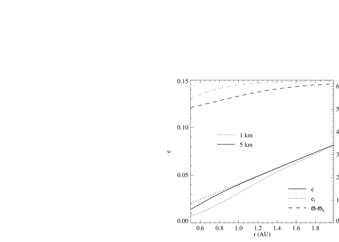
Figure 1: Axisymmetric gas disc case ($e_{\mathrm{g}}=0$). Equilibrium eccentricity (solid curves) and $\varpi$ (dashed curves) distributions for $e_{\mathrm{b}}=0.3$, $a_{\mathrm{b}}=10$ AU and $q_{\mathrm{b}}=0.5$ (tight binary case) for planetesimals of 1 km (black curves) and 5 km (gray curves), as given by Eqs. (28) and (29). Also shown is the forced eccentricity $e_{\mathrm{f}}$ (black dotted line).

3.3 Non-linear drag

A linear drag force is not appropriate for planetesimals. For large bodies, a non-linear drag force is more appropriate:

$${\vec{f}_{\mathrm{drag}}}=-K\left|{\vec{\Delta}v}\right|{\vec{\Delta}v},$$ (18)

where

$$K=\frac{3\rho_{\mathrm{g}}}{20\rho_{\mathrm{pl}}R},$$ (19)

where $\rho_{\mathrm{g}}$ is the gas density, $\rho_{\mathrm{pl}}$ is the internal density of the planetesimals, and $R$ is the planetesimal radius. We have assumed the planetesimals to be spherical. For this drag law, the drag term Eq. (15) gets replaced by

$$-\sqrt{5}Kr\Omega^{2}\left|E-E_{\mathrm{g}}\right|\left(E-E_{\mathrm{g}}\right).$$ (20)

In this case it is not feasible to obtain an expression for the time evolution of the eccentricity, but we can still look at the stationary solution, which is given by:

$$\frac{3q_{\mathrm{b}}}{2\left(1-e_{\mathrm{b}}^{2}\right)^{3/2}}\left(\frac{r}{a_{\mathrm{b}}}\right)^{3}E_{0}+i\sqrt{5}Kr\left|E_{0}-E_{\mathrm{g}}\right|\left(E_{0}-E_{\mathrm{g}}\right)\\ -\frac{15e_{\mathrm{b}}q_{\mathrm{b}}}{8\left(1-e_{\mathrm{b}}^{2}\right)^{5/2}}\left(\frac{r}{a_{\mathrm{b}}}\right)^{4}=0.$$ (21)

If we write $z=E_{0}-E_{\mathrm{g}}$, then

$$z+i\mathcal{K}\left|z\right|z+E_{\mathrm{g}}-e_{\mathrm{f}}=0,$$ (22)

with

$$\mathcal{K}=\frac{2\sqrt{5}Kr\left(1-e_{\mathrm{b}}^{2}\right)^{3/2}}{3q_{\mathrm{b}}\left(\frac{r}{a_{\mathrm{b}}}\right)^{3}}.$$ (23)

Then it is straightforward to show that in this case

$$E_{0}=e_{\mathrm{f}}+\left(E_{\mathrm{g}}-e_{\mathrm{f}}\right)\frac{Z-1+i\sqrt{2Z-2}}{Z+1},$$ (24)

where

$$Z=\sqrt{1+4\mathcal{K}^{2}\left|E_{\mathrm{g}}-e_{\mathrm{f}}\right|^{2}}$$ (25)

All size-dependence is contained in $Z$, and it is clear that again for the special case $E_{\mathrm{g}}=e_{\mathrm{f}}$ there is no differential orbital phasing. Also for this case we expect small encounter velocities.

For completeness, we write out the magnitude $e_{0}$ and the argument $\varpi_{0}$ of the complex equilibrium eccentricity $E_{0}$:

$$e_{0}^{2}=\frac{2e_{\mathrm{f}}^{2}+(Z-1)e_{\mathrm{g}}^{2}-2\sqrt{2Z-2}e_{\mathrm{f}}\mathcal{I}(E_{\mathrm{g}})}{Z+1},$$ (26)

$$\tan(\varpi_{0})=-\sqrt{\frac{Z-1}{2}}\\ \frac{(Z-1)\mathcal{I}(E_{\mathrm{g}})-\sqrt{2Z-2}(e_{\mathrm{f}}-\mathcal{R}(E_{\mathrm{g}}))}{(Z-1)\mathcal{I}(E_{\mathrm{g}})-\sqrt{2Z-2}\left(e_{\mathrm{f}}+\mathcal{R}(E_{\mathrm{g}})\frac{Z-1}{2}\right)},$$ (27)

where $\mathcal{R}(E_{\mathrm{g}})$ and $\mathcal{I}(E_{\mathrm{g}})$ denote respectively the real and imaginary part of $E_{\mathrm{g}}$ and $e_{\mathrm{g}}$ its absolute value. The last two expressions lead to two interesting observations. When the gas disc eccentricity vector has a significant positive imaginary part, the eccentricity of the particles is reduced. This happens when the gas disc is not aligned (or anti-aligned) with the binary orbit. For the special case $Z=3$ and $E_{\mathrm{g}}=ie_{\mathrm{f}}$ we have $E_{0}=0$. Though this may seem a pathological case, we will see that this behavior actually shows up in the numerical simulations.

The case of a circular gas disc (defined as having $e_{\mathrm{g}}=0$, but not necessarily being axi-symmetric) appears to be particularly simple:

$$e_{0}=\sqrt{\frac{2}{1+Z}}e_{\mathrm{f}}$$ (28)

$$\tan(\varpi_{0})=-\sqrt{\frac{Z-1}{2}}.$$ (29)

In the inner regions of the disc, where gas drag is very strong and therefore $Z\gg 1$, the eccentricity will be much smaller than $e_{\mathrm{f}}$, while the longitude of periastron will make a 90-degree angle with that of the binary. This effect can be clearly seen in Fig. 6 of Thébault et al. (2006) (also see our Fig. 5). As $Z\rightarrow 1$, indicating less friction (either due to a lower gas density or a larger particle size), particles tend to adopt the forced eccentricity and align with the binary. Note, however, that this analysis does not take into account the oscillatory behavior of $E$, and is therefore only valid for $Z\gg 1$ or at sufficiently late times. We show the resulting eccentricity distribution for $q_{\mathrm{b}}=0.5$, $e_{\mathrm{b}}=0.3$ and $a_{\mathrm{b}}=10$ AU in Fig. 1. These results compare very well to the numerical results (see Fig. 5).

In the limit $e_{\mathrm{f}}\ll\sqrt{Z-1}e_{\mathrm{g}}$, some simple relations can be obtained:

$$e_{0}=\sqrt{\frac{Z-1}{Z+1}}e_{\mathrm{g}}$$ (30)

$$\tan(\varpi_{0})=\frac{\tan(\varpi_{\mathrm{g}})+\sqrt{\frac{2}{Z-1}}}{1-\sqrt{\frac{2}{Z-1}}\tan(\varpi_{\mathrm{g}})},$$ (31)

where $\varpi_{\mathrm{g}}$ denotes the longitude of periastron of the gas disc. We see that in the limit of strong coupling to the gas ($Z\gg 1$), the planetesimals will tend to obtain the gas disc eccentricity. On the contrary, for very weak coupling ($Z\rightarrow 1$), their eccentricity will tend to zero. Note, however, that Eq. (30) is not valid in the limit $Z\rightarrow 1$; from Eq. (26) it is in fact easy to see that $e_{0}\rightarrow e_{\mathrm{f}}$ for $Z\rightarrow 1$.

An important conclusion is that, except in the special case $E_{\mathrm{g}}=e_{\mathrm{f}}$, friction with an eccentric gas disc always leads to some degree of differential orbital phasing between planetesimals of different sizes. This case is thus qualitatively not different from that of a circular gas disc. The magnitude of the differential orbital phasing effect will depend strongly on the gas eccentricity though.

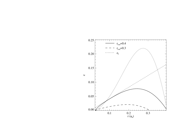
Figure 2: Equilibrium gas eccentricity distribution, analytically derived from Eq. (32), for $e_{\mathrm{b}}=0.3$, and $q_{\mathrm{b}}=0.5$ with $\beta=-7/4$ (gray curve) or $q_{\mathrm{b}}=0.234$ with $\beta=-1/2$ (black curves). Also shown is the forced eccentricity $e_{\mathrm{f}}$ (black dotted line), which is the same for both cases. The dashed black curve shows the effect of moving the outer boundary inwards. All models use $h=0.05$.

3.4 Gas disc eccentricity

We now consider the crucial issue of the response of the gas disc itself to the perturbations. The equivalent of Eq. (6) for a gaseous disc reads:

$$-\frac{2i}{h^{2}\Omega}\frac{\partial E_{\mathrm{g}}}{\partial t}=r^{2}E_{\mathrm{g}}^{\prime\prime}+(2+\beta)rE_{\mathrm{g}}^{\prime}+\\ \left(\beta-1+\frac{3q_{\mathrm{b}}}{2h^{2}\left(1-e_{\mathrm{b}}^{2}\right)^{3/2}}\left(\frac{r}{a_{\mathrm{b}}}\right)^{3}\right)E_{\mathrm{g}}\\ -\frac{15e_{\mathrm{b}}q_{\mathrm{b}}}{8h^{2}\left(1-e_{\mathrm{b}}^{2}\right)^{5/2}}\left(\frac{r}{a_{\mathrm{b}}}\right)^{4},$$ (32)

where $\beta\equiv d\log\Sigma/d\log r$, $h=H/r$, and primes denote differentiation with respect to $r$. It is possible to find equilibrium solutions by setting the left-hand side to zero, after which the resulting second order ordinary differential equation can be solved in terms of Bessel functions (for constant $\beta$). Before doing so, we note that for the case $\beta=-1/2$, $E_{\mathrm{g}}=e_{\mathrm{f}}$ is actually a solution (for appropriate boundary conditions).

It is not straightforward to supply realistic boundary conditions for this problem. It is conceivable that the gas disc eccentricity will tend to zero close to the star, and numerical hydrodynamical simulations (to which we intend to compare these results) will also force the eccentricity to be zero at the boundaries. Therefore we choose $E_{\mathrm{g}}(r_{\mathrm{in}})=0$, where $r_{\mathrm{in}}$ is the inner radius of the disc. The outer boundary poses a bigger problem, because the disc will be truncated. Since linear theory does not include the truncation of the disc, we vary the outer boundary condition between $E_{\mathrm{g}}(r_{\mathrm{out}})=0$, where $r_{\mathrm{out}}$ is the outer radius of the disc and $E_{\mathrm{g}}(r_{\mathrm{trunc}})=0$, where $r_{\mathrm{trunc}}$ is the approximate truncation radius of the disc, obtained from hydrodynamical simulations. Note that since $\varpi(r_{\mathrm{in}})=\varpi(r_{\mathrm{out}})=0$, the disc will be aligned with the binary everywhere according to Eq. (32). A possible twist in the disc does not change the results significantly.

Figure 3: Circular gas disc case, for a tight binary $q_{\mathrm{b}}=0.5$, $e_{\mathrm{b}}=0.3$ and $a_{\mathrm{b}}=10$ AU. Shown are analytical estimates of mean encounter velocities between planetesimals, at $1$ AU from the primary, as a function of their size, derived using Eq. (33). We consider target bodies of two different sizes, one with $R=1\,$km and the other $R=5\,$km, and derive for each case collision velocities due to impacting objects in the $1$-$10$ km size range. Overplotted are the results of Thébault et al. 2006 (their Table $3$).

The results are shown in Fig. 2, for two binary configurations: $q_{\mathrm{b}}=0.5$, $e_{\mathrm{b}}=0.3$, $\beta=-7/4$ (gray curve), and $q_{\mathrm{b}}=0.234$, $e_{\mathrm{b}}=0.3$, $\beta=-1/2$ (black curves). Both cases will be studied numerically in Sect. 5. We put the boundaries at $r_{\mathrm{in}}=0.025$ $a_{\mathrm{b}}$ and $r_{\mathrm{out}}=0.4$ $a_{\mathrm{b}}$, the same as will be used in Sect. 5 in the hydrodynamical simulations. For these binary parameters, the outer boundary is well beyond the truncation radius, while the inner boundary is well inside the planet-forming region (for $a_{\mathrm{b}}\sim 10$ AU).

The steep density profile (denoted by the gray curve in Fig. 2) gives rise to an eccentricity well above $e_{\mathrm{f}}$ for a large part of the disc. Reducing the inner radius of the disc by a factor of 2 has virtually no effect on the eccentricity. This is not true for the outer boundary, as we will see below. For $\beta=-1/2$, the eccentricity approaches $e_{\mathrm{f}}$ far from the boundaries. This may be important, because in this case there would be no differential orbital phasing in the planet-forming region. However, this strongly depends on the location of the outer boundary. If we suppose that the disc is circular at the truncation radius, which, for this binary configuration, is located around $r_{\mathrm{trunc}}=0.3$ $a_{\mathrm{b}}$, the picture changes drastically (see the dashed line in Fig. 2). In this case, the disc remains nearly circular everywhere, and we will see in Sect. 5 that this closely resembles the solution obtained from numerical hydrodynam ical simulations. Also, there is a strong dependence on $h$, with larger eccentricities for thinner discs.

However, there are three possibly important physical effects not included in Eq. (32). First of all, tidal effects are neglected, which means that the effect of disc truncation is not taken into account. Therefore $\beta=\beta(r)$ is unknown, and will change dramatically near the disc edge.

There are also two possible eccentricity excitation mechanisms not included in Eq. (32). There is the effect of the 3:1 resonance (Lubow, 1991), and also the viscous overstability (Kato, 1978; Latter & Ogilvie, 2006). Both mechanisms can add a significant free eccentricity to the disc. We rely on numerical hydrodynamical simulations to solve for the eccentricity of the gas disc.

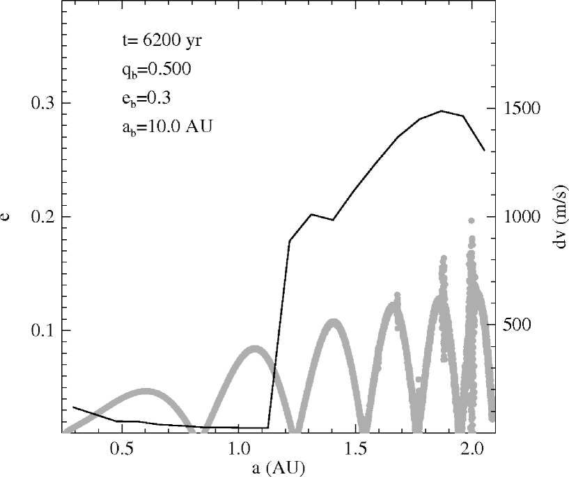
Figure 4: Planetesimal eccentricity (grey dots) and average encounter velocity (solid line) distribution in a gas-free disc, for the tight binary case.

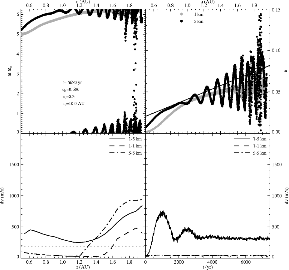
Figure 5: Planetesimal evolution in an axisymmetric gas disc, with $\Sigma_{0}\propto r^{-7/4}$ for the same binary parameters as in Fig. 4 (see also the top left panel). Top left: longitude of periastron distribution after 5680 yr. Top right: eccentricity distribution after 5680 yr, with the black line indicating the forced eccentricity $e_{\mathrm{f}}$. Bottom left: distribution of encounter velocities for 3 different impactor-target planetesimal pairs: 2 corresponding to equal sized impacting objects and the third one to a 1 km impactor hitting a 5 km target. Also shown is the limiting maximum $\langle dv\rangle$ for accreting encounters between 1 and 5 km bodies (dotted line). Bottom right: encounter velocities at 1 AU as a function of time for the same impactor-target pairs.

3.5 Encounter velocities

A simple model, where one considers the collision between two kinds of bodies with the same semi-major axis in the guiding centre approximation, suggests that their mean encounter velocity is proportional to $|E_{1}-E_{2}|$. If we take

$$\overline{|\Delta{\vec{v}}|}=a\Omega\sqrt{\frac{5}{8}}|E_{1}-E_{2}|,$$ (33)

then this prediction reduces to the standard relation for bodies with mean eccentricity $e_{\mathrm{f}}$ and randomized periastra of Lissauer & Stewart (1993):

$$\overline{|\Delta{\vec{v}}|}=a\Omega\sqrt{\frac{5}{4}}e_{\mathrm{f}}.$$ (34)

When assuming a given eccentricity $E_{\mathrm{g}}$ for the gas disc, Eq. (33), together with Eq. (24), can be used to predict the stationary solution for mutual encounter velocities. For the specific case of a circular gas disc, it gives a remarkably good fit to the numerical results obtained, once the stationary state is reached, by Thébault et al. (2006) (Fig. 3). Note however that this set of equations cannot predict if, and how fast the stationary state will be reached. It also cannot account for the possibly crucial effect of encounters due to high-eccentricity objects coming from other regions of the system (in case of orbital crossing). These equations are nevertheless very useful in providing a reference to which to compare numerical results obtained with an evolving gas disc. Such a comparison can provide information on whether the gas disc eccentricity dominates the collisional evolution of the planetesimal population.

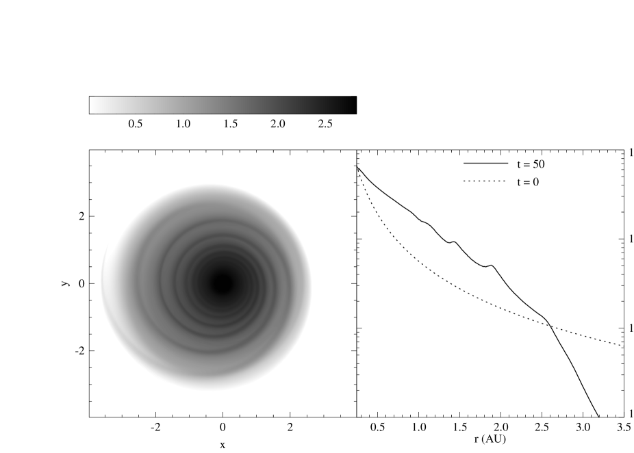
Figure 6: Surface density of the gas disc, with $\Sigma_{0}\propto r^{-7/4}$ after 50 binary orbits ($\approx 1600$ yr), for the same binary parameters as in Fig. 4. Left panel: two-dimensional distribution of $\log_{10}\Sigma$. The binary companion is at apo-astron, at $(x,y)=(-13,0)$. Right panel: azimuthally averaged surface density. The density scale is arbitrary, for comparison the initial condition is shown.

4 Test cases: gas free and axisymmetric cases

We start by reproducing the results of Thébault et al. (2006) for the gas-free case and for an axisymmetric gas disc. These results can then serve as a reference for the full model, but they also provide good test cases for our method.

Figure 7: Gas disc eccentricity (top panel) and longitude of periastron (bottom panel) for the excited state, obtained with the soft superbee flux limiter (solid line) and the quiet state, obtained with the minmod flux limiter (dotted line). The binary parameters correspond here to the wider binary case of $\gamma$ Cephei: $q_{\mathrm{b}}=0.234$, $a_{\mathrm{b}}=20$ AU, $e_{\mathrm{b}}=0.3$, and the initial surface density has a shallow radial dependence $\Sigma_{0}\propto r^{-1/2}$. The thick solid line indicates the forced eccentricity derived from Eq. (12).

Figure 8: Evolution of the mean disc eccentricity and longitude of periatron, for the wide binary case $q_{\mathrm{b}}=0.234$, $e_{\mathrm{b}}=0.3$ and $a_{\mathrm{b}}=20$ AU, with $\Sigma_{0}\propto r^{-1/2}$, using two different flux limiters.

4.1 Gas-free disc

In the case of no gas drag, the eccentricity evolution of the planetesimals is governed by secular perturbations due to the binary only. These perturbations give rise to eccentricity oscillations, with a wavelength that decreases with time. Due to the strong orbital phasing large eccentricities may arise with relatively low encounter velocities. However, as time goes by the eccentricity oscillations become so narrow that orbital crossing between high and low eccetricity bodies eventually occur, resulting in a sudden and dramatic increase of encounter velocities. Orbital crossing first occurs in the outer regions (closer to the companion star), the radial location at which orbital crossing occurs progressively moving inward with time. The time at which orbital crossing occurs at a given location can be calculated analytically following the empirical derivation of Thébault et al. (2006).

In Fig. 4 we show the eccentricity distribution of planetesimals after 6200 yr (200 binary orbits) in a tight binary system with parameters as indicated above the figure. The eccentricity oscillation can be identified easily. In the outer part of the disc, several particles have been captured into resonances. Note that we only consider here the inner $\leq 2$ AU part of the disc, since most planetesimal orbits beyond this distance are dynamically unstable.

The black solid line in Fig. 4 indicates the mean encounter velocities as a function of distance. The radius where orbital crossing occurs can be found near $1.1$ AU (note the very sharp transition from $\langle\Delta v\rangle\simeq 0$ to very high velocity values in less than $0.1$ AU around the crossing location. These results quantitatively agree with the calculations of Thébault et al. (2006) (see their Fig. 2).

4.2 Axisymmetric gas disc

Thébault et al. (2006) included effects of gas drag from an axisymmetric gas disc. In this section, we use the same gas disc model as Thébault et al. (2006) and do not let it evolve. We divide the 10000 planetesimals into two groups of 1 km and 5 km in size. We consider the same tight binary configuration as in the gas free case: $a_{\mathrm{b}}=10\,$, $e_{\mathrm{b}}=0.3$ and $q_{\mathrm{b}}=0.5$. In Fig. 5, we show the resulting orbital and collisional evolution, in the $\leq 2$ AU region corresponding to stable orbits. These can be compared to Figs. 6 and 7 of Thébault et al. (2006).

In the top panels of Fig. 5, we observe the well known (e.g. Marzari & Scholl, 2000; Thébault et al., 2004) double effect of gas drag on planetesimal orbits, i.e., damping of the eccentricities and periastron alignment. At first sight, this may seem advantageous for planetesimal accretion. However, the equilibrium between eccentricity excitation and damping depends on the size of the planetesimals. Not only are the eccentricities of the smaller bodies damped more readily than for the larger bodies, they are damped towards a different equilibrium. This is also true for the equilibrium value of the periastron alignment. This differential phasing is responsible for high collision velocities between particles of different sizes (Thébault et al., 2006). Note also that in the inner disc, where the eccentricity oscillations are damped by gas friction, the eccentricities and longitudes of periastron of the planetesimals agree with the analytical results in Fig. 1 .

These consequences of gaseous friction are clearly illustrated in the bottom panels of Fig. 5 which shows the evolution of the average encounter velocities $\langle\Delta v\rangle_{R1,R2}$, for the cases $R_{1}=R_{2}=1$ km, $R_{1}=R_{2}=5$ km, $R_{1}=1$ km and $R_{2}=5$ km. A first obvious effect, clearly seen for the case of equal-sized objects, is that gas drag works against orbital crossing: stronger gas friction moves the radius at which orbital crossing occurs outward. At 1 AU, no orbital crossing occurs after 3000 yr for both planetesimal sizes and relative velocities are still very low (see the bottom left panel of Fig. 5). In sharp contrast, encounter velocities between bodies of different size are high throughout the disc. In the bottom right panel of Fig. 5, we see that the encounter velocities reach a stationary value after approximately 5000 years. The equilibrium is in perfect agreement with the result from Thébault et al. (2006). In the bottom left panel of Fig. 5 we also show the limiting value of $\langle dv\rangle$ for accreting collisions between planetesimals of 1 and 5 km (dotted line). This is a conservative estimate, based on the most optimistic value for accretion considered by Thébault et al. (2006).

5 Results, full model

5.1 Gas disc evolution

We start the discussion of the full model by considering the gas evolution alone. In Fig. 6 we show the surface density of the gas disc after 50 binary orbits using the minmod flux limiter. The disc is truncated by the binary at approximately the radius predicted by the empirical formula of Holman & Wiegert (1999). A large part (approximately $20\%$) of the material is expelled from the system, but from the right panel of Fig. 6 it is also clear that the disc is compressed: the density at 1 AU is increased by approximately a factor of 3. This means that in order to compare with the results of the previous section, we should rescale the density in the full model to obtain the same magnitude of the drag force at 1 AU.

The second thing that is apparent from Fig. 6 is the appearance of spiral density waves. The morphology is strongly dependent on the phase of the binary (see Kley & Nelson, 2007), with strong shocks appearing just after periastron. The effect of these waves in a circular binary on the orbital elements of planetesimals was recently studied in Ciecielag et al. (2007), where it was shown that only the smallest bodies ($R\approx 100$ m) are affected.

Finally, it is clear from the left panel of Fig. 6 that the gas disc becomes eccentric. This is always true, but tests show that the two considered flux limiters give very different results. The amplitude of the eccentricity increase depends dramatically on the amount of wave damping, as is illustrated in Fig. 7, where we compare the eccentricity distribution after 50 binary orbits for the $\gamma$ Cephei binary configuration, ($q_{\mathrm{b}}=0.234$, $a_{\mathrm{b}}=20$ AU, $e_{\mathrm{b}}=0.3$) for results obtained with our two different flux limiters.

The diffusive minmod limiter gives rise to a low eccentricity ($e_{\mathrm{g}}\leq 0.05$ and even $\leq 0.02$ in $r<4$ AU region), stationary disc state that we henceforth call the quiet state. It is a robust state, numerically, to changes in resolution and boundary conditions (reflecting, non-reflecting). In fact, this solution approximately obeys the time-independent version of Eq. (32), as we will show below. The maximum eccentricity does depend on the location of the inner boundary, however, since the boundary conditions enforce the eccentricity to be zero at the boundary. We have found that the location of the inner boundary should be at least as far in as $0.025$ $a_{\mathrm{b}}$ to get converged results.

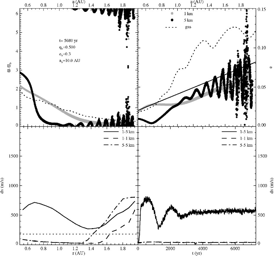
Figure 9: Planetesimal evolution in an evolving gas disc (the quiet state), with a steep radial gas profile in $\Sigma_{0}\propto r^{-7/4}$, for the same tight binary parameters as in Fig. 5. Top left: longitude of periastron distribution after 5680 yr. Top right: eccentricity distribution after 5680 yr. Bottom left: distribution of encounter velocities for 3 different impactor-target planetesimal pairs: 2 corresponding to equal sized impacting objects and the third one to a 1 km impactor hitting a 5 km target. Also shown is the limiting $\langle dv\rangle$ for accreting encounters (dotted line). Bottom right: encounter velocities at 1 AU as a function of time for the same 3 impactor-target pairs.

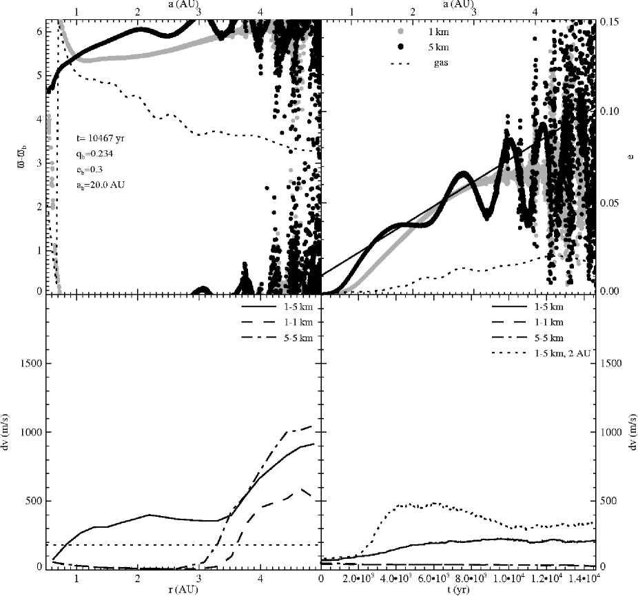
Figure 10: Planetesimal evolution in an evolving gas disc (the quiet state), with a shallower radial gas profile $\Sigma_{0}\propto r^{-1/2}$, and for the wider, $\gamma$ Cephei like binary case. Top left: longitude of periastron distribution. Top right: eccentricity distribution. Bottom left: distribution of encounter velocities for 3 different impactor-target planetesimal pairs: 2 corresponding to equal sized impacting objects and the third one to a 1 km impactor hitting a 5 km target. Also shown is the limiting $\langle dv\rangle$ for accreting encounters (dotted line). Bottom right: encounter velocities at 1 AU as a function of time for the same 3 impactor-target pairs. In addition, we show the encounter velocities at 2 AU for a 1 km impactor hitting a 5 km target (dotted line).

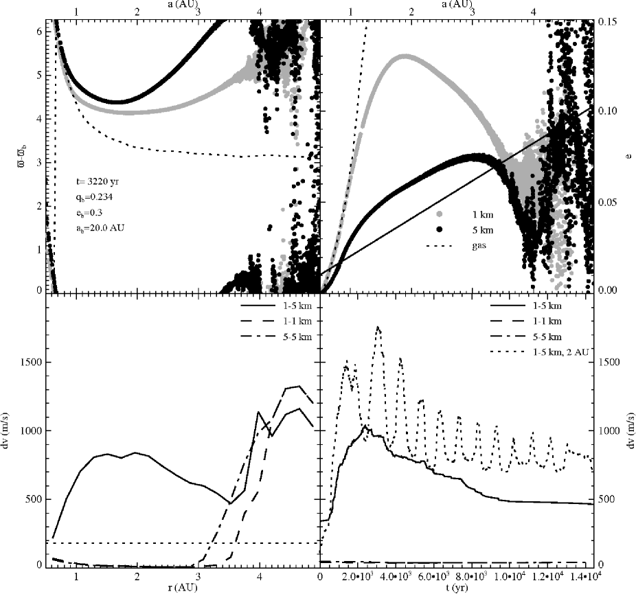
Figure 11: Planetesimal evolution in an evolving gas disc (the excited state), with $\Sigma_{0}\propto r^{-1/2}$, for the same binary parameters as in Fig. 10. Top left: longitude of periastron distribution. Top right: eccentricity distribution. Bottom left: distribution of encounter velocities for 3 different impactor-target planetesimal pairs: 2 corresponding to equal sized impacting objects and the third one to a 1 km impactor hitting a 5 km target. Also shown is the limiting $\langle dv\rangle$ for accreting encounters (dotted line). Bottom right: encounter velocities at 1 AU as a function of time for the same 3 impactor-target pairs. In addition, we show the encounter velocities at 2 AU for a 1 km impactor hitting a 5 km target (dotted line).

The soft superbee flux limiter gives rise to a different disc state, with a large free eccentricity, reaching values up to $e_{\mathrm{g}}\sim 0.2$. We will refer to this state as the excited state. This state is similar to the one discussed in Kley & Nelson (2007). Its exact behavior depends strongly on resolution and boundary conditions, but the overall picture is the same: high eccentricity, and the disc starts to precess. This is illustrated in Fig. 8, where we show the mass-averaged eccentricity and longitude of periastron for the disc. Within 20 orbits, the disc obtains a large eccentricity, after which the disc starts to precess slowly in a retrograde fashion. The eccentricity oscillates with the same period as the precession. The retrograde precession indicates that pressure forces are dominant (see Papaloizou, 2005). In Fig. 8, the quiet disc quickly reaches a steady eccentricity distribution. Note that due to the twist in the disc (see Fig. 7), which is dynamically unimportant, the average longitude of periastron approaches neither $0$ nor $\pi$, but somewhere in between.

Note that for both states the disc eccentricity does not equal the forced eccentricity, denoted by the thick solid line in Fig. 7. For the quiet state, we have checked that the gas eccentricity approximately follows Eq. (32). The fact that, despite the density being proportional to $r^{-1/2}$, the gas eccentricity does not tend to the forced eccentricity is due to the behavior near the truncation radius. This is basically where the boundary condition for Eq. (32) is determined, which, as shown in Fig. 2 can easily lead to a strongly reduced disc eccentricity. According to the analytical study of Sect. 3, this means that we can expect large encounter velocities between planetesimals in both cases.

The reason for the large differences between the runs with different flux limiters is that the mechanism responsible for generating a large free eccentricity involves an eccentric resonance near the outer edge of the disc. Basically, it is the mechanism outlined in Lubow (1991), but for an eccentric companion orbit. Heemskerk (1994) showed that eccentricity excitation through this instability strongly depends on the way the disc is truncated, which in turn depends strongly on wave damping. The two different limiters give different wave damping, hence our results, see Appendix A. Only for small wave damping does the disc obtain a large free eccentricity. It is expected that this also depends on the magnitude of the physical viscosity, since this affects the shape of the disc edge. We provide some additional comments in Sect. 6, but leave a detailed discussion of this problem to a future publication. We now proceed to analyze the influence of both disc states on planetesimal accretion.

5.2 Planetesimal evolution

5.2.1 Quiet disc case

We first consider the quiet disc case, for which the situation should a priori be the closest to the non-evolving axisymmetric case.

Fig. 9 shows the evolution of planetesimal orbital parameters and encounter velocities for the same tight binary parameters as in Fig. 5. Comparing the top panels of Figs. 5 and 9 we see that, as expected, the largest differences occur in the inner regions of the disc, typically within $\sim 0.8$ AU, where gas drag effects are the most important. The 1-km planetesimals approach the gas eccentricity towards the inner boundary, as expected. Interestingly, the 5-km bodies show a large jump in longitude of periastron around $r=0.7$ AU, accompanied by a drop in eccentricity. From the top left panel of Fig. 9 we see that this happens where the longitude of periastron of the gas disc amounts to $\pi/2$. Around this location, depending on the value of $Z$, the denominator of Eq. (27) will approach zero, causing a large jump in $\varpi$. For the 5 km planetesimals, $Z\approx 3$ at this location, which causes a drop in eccentricity (see Eq. (26)). This is not true for the 1 km planetesimals, and therefore there is a large eccentricity difference around $r=0.7$ AU.

In terms of encounter velocities, these different behaviours of 1 and 5 km bodies in the innermost regions logically translate into higher $\Delta v$ than in the axisymmetric case (see the bottom-left panel of Figs. 5 and 9). At 1 AU, the equilibrium encounter velocities are approximately a factor of 2 higher than for the case of a circular gas disc. However, in the outer disc, beyond $\sim$1 AU, differences with the axisymmetric case are much smaller. Although the gas eccentricity is higher in these regions, the gas density is not high enough to significantly affect the behaviour of km-sized planetesimals. Beyond $r=1.4$ AU, the dynamical evolution of the planetesimal population becomes indistinguishable from the circular gas disc case.

We now turn our attention to binary parameters that match those of $\gamma$ Ceph: $q_{\mathrm{b}}=0.234,a_{\mathrm{b}}=20$ AU and $e_{b}=0.3$. From Fig. 7 we see that the gas disc eccentricity is very small, $e_{\mathrm{g}}<0.02$ almost everywhere. In the top panels of Fig. 10 we show the distribution of longitude of periastron and eccentricity after $10^{4}$ yr, when the system has reached a steady state. We find that in the whole $r\geq 0.8$AU region, the equilibrium $\langle\Delta v\rangle$ for collisions between 1 and 5 km objects is $\geq 200\,$m s^-1. This is still high enough to correspond to eroding impacts for all tested collision outcome prescriptions of Thébault et al. (2006) (see bottom-left panel of Fig.10). Direct comparison with Fig. 5 is here difficult, because the binary parameters are different. We thus performed an additional axisymmetric gas disc test simulation which showed that the encounter velocities are the same, within $10\%$, as for the present quiet state run. This is an indication that the spiral waves, that do extend all the way in, are indeed of minor importance regarding impact velocities. The circular gas disc case is then a relatively good approximation.

5.2.2 Excited disc case

In Fig. 11 we show the results for the excited disc state, for the $\gamma$ Cephei like binary. It is immediately clear that, even for this wide binary case, the planetesimals react rather violently to the large eccentricity of the gas disc. Inside 1 AU, the 1 km planetesimals are dragged along with the gas and end up on highly eccentric orbits matching that of the gas. The 5 km planetesimals follow the same trend, but are more loosely coupled to the gas streamlines and their eccentricities never match that of the gas. For the periastra, however, we observe a quasi-perfect alignment with that of the gas for both planetesimal sizes. Note that this rather abruptly happens where $\varpi_{\mathrm{g}}\approx 3\pi/2$, which makes $|\tan(\varpi_{\mathrm{g}})|$ very large. From Eq. (31) we see that in this case, for which we indeed have $e_{\mathrm{g}}\gg e_{\mathrm{f}}$, we expect all planetesimals to align with the gas, independently of $Z$. Outside 1 AU, 1 km planetesimals start to decouple from the gas, while the bigger bodies do so already at $\sim 0.7$ AU. In the whole $1\leq r\leq 3\,$AU region, differences between the equilibrium eccentricities for both sizes are very large, culminating at $\sim 2\,$AU, where $e_{\mathrm{1km}}\approx 2\,e_{\mathrm{5km}}$.

The differences in $E$ between the two particle sizes in the planet-forming region around 1 AU lead to very high encounter velocities, exceeding $500\,$m s^-1 almost everywhere (bottom panel of Fig. 11). Note that due to the precession of the disc, $E_{\mathrm{g}}$ is time dependent, as appears clearly from the oscillations in Fig. 8. However, this precession timescale is shorter than the time it takes for the planetesimals to settle into their equilibrium distribution. Therefore, the planetesimals will feel an average gas eccentricity and eventually settle into a steady eccentricity and $\langle\Delta v\rangle$ distribution. Also, the disc at 1 AU does not really participate in the precession, possibly due to the fact that it is close to the inner boundary (see also below). This is also apparent from Fig. 7. For comparison, we also show the encounter velocities evolution at 2 AU in the bottom right panel of Fig. 11. We see that, at this larger distance, the encounter velocities oscillate, with a period which is that of the gas disc precession (see Fig. 8), but after approximately $10^{4}$yrs a meaningful average can be defined. We note that, at a given location in the disc, encounter velocities are close to those predicted by Eq. (33), when plugging in the average value of $E_{\mathrm{g}}$ at this location (see also Fig. 12). This again shows that it is the eccentricity of the gas disc that governs the impact velocities.

The bottom left panel of Fig. 11 shows that encounter velocities in the inner regions, which are due to (gas drag induced) differential orbital phasing, come close to those in the outer disc, which are due to pure gravitational orbital crossing. For 1km-5km pairs, impact velocities are on average 5 times higher than those in the circular disc run. They are thus far above the upper limit for accreting impacts for the whole simulated region $0.6<r<6\,$AU.

We have also run the soft superbee flux limiter for the tight binary case. Differences with the circular case are slightly larger than for the quiet state, but the gas disc is not able to obtain a large free eccentricity in this case, for two reasons. First, numerical and analytical experiments suggest that the maximum eccentricity (free or forced) that the gas disc can reach is largely determined by the boundaries (see also Fig. 2). The quiet state of the tight binary comes close to obtaining this maximum of $e_{\mathrm{g}}\sim 0.3$, and therefore the excited state is not very much different in this case. Second, because the gas disc is truncated closer to the primary, due to the stronger perturbations from the tight binary, the mechanism for generating a large free eccentricity is reduced in strength compared to the wide binary case. Therefore, encounter velocities do not vary more than $50\,\%$ between the quiet and excited state for the tight binary, meaning that velocities are here a factor of $\sim 3$ higher than in the circular gas disc case.

As already mentioned, numerical experiments have shown that the position of the inner boundary determines up to what radius the gas disc obtains its large eccentricity. For example, in Fig. 7, the eccentricity drop inward of 2 AU is directly connected to the location of the inner boundary at $0.25\,$ AU. Exploring this parameter is outside the scope of the present paper, since moving the inner boundary further inwards is computationally very expensive. However, it is important to note that it would only act to further increase the encounter velocities. More work is necessary to study the behavior of the excited disc state close to the inner edge of the disc, numerical or physical. Here, we focus on the influence of a gas disc with a large free eccentricity on planetesimal collisions only, and we have shown that it is disastrous for planetesimal growth.

Figure 12: Encounter velocities, calculated using Eq. (33) for the mean eccentricity of the excited gas disc state, for binary parameters $q_{\mathrm{b}}=0.234$, $a_{\mathrm{b}}=20$ AU and $e_{b}=0.3$. Black lines were calculated using $E_{\mathrm{g}}=0.05$, appropriate for 1 AU (see Fig. 7), grey lines using $E_{\mathrm{g}}=0.15$, appropriate for 2 AU.

6 Discussion

6.1 The impact of gas disc eccentricity on encounter velocities

Our results indicate that planetesimal encounter velocities, which result from differential orbital phasing due to gas drag, critically depend on the eccentricity of the gas disc. Although there is a theoretical possibility for differential phasing to be avoided, when gas streamlines follow the forced dynamical orbits, we have shown that this situation does not occur in practice. First of all, Eq. (32) shows that we can only have $E_{\mathrm{g}}=e_{\mathrm{f}}$ when the gas density follows $\Sigma\propto r^{-1/2}$. Even if this happens to be the case, there is a strong dependence on what happens at the inner and outer boundaries of the disc (see Fig. 2), in combination with the disc thickness. More importantly, this $E_{\mathrm{g}}=e_{\mathrm{f}}$ condition was never encountered in our numerical hydrodynamical simulations. Since we could not explore all free parameters, we cannot rule out the possibility of obtaining $E_{\mathrm{g}}=e_{\mathrm{f}}$ very locally when tuning in the right disc parameters, but this would have to be a fortuitous coincidence. Even more, if the disc reaches a large free eccentricity, then it will necessarily precess, so that $E_{\mathrm{g}}=e_{\mathrm{f}}$ would not be a steady state.

Not only does this $E_{\mathrm{g}}=e_{\mathrm{f}}$ state never occur, but for all 4 cases here explored (2 flux limiters + 2 binaries configurations), we always obtain, at all radial distances, $\langle\Delta v\rangle$ equilibrium values higher than for a static circular gas disc case. For the quiet state, differences with the static case remain relatively limited: velocity distributions are almost identical for a binary with $20\,$AU separation and are enhanced by slightly less than a factor of 2 for a tight $a_{\mathrm{b}}=10$ AU companion. For the excited state, however, differences with the static disc case can become large. They already exceed a factor of 2 for the wide (20 AU) binary case and reach a factor of 3 for the tight binary. Interestingly, even for the case where $e_{\mathrm{g}}$ turns out be relatively close to $e_{\mathrm{f}}$, i.e., in the inner disc in the quiet state/tight binary run (see Fig. 9), we still observe an important differential phasing between particles of different sizes and thus high $\langle\Delta v\rangle$ values. This is entirely due to the fact that the gas disc is not aligned with the binary in that region. This is a further indication that the parameter phase space around the exact $E_{\mathrm{g}}=e_{\mathrm{f}}$ condition where differential phasing is weaker than for a circular disc is very limited.

The computational cost of the presented numerical simulations inhibits an extended parameter study similar to the one in Thébault et al. (2006) for the static circular gas disc case. As already mentioned, we had to restrict ourselves to two representative binary configurations as well as to two planetesimal sizes, 1 and 5 km. However, we have checked (see Fig.12) that for all numerically explored cases, Eq. (33) gives good estimates of equilibrium encounter velocities once given the value for the mean gas disc eccentricity $E_{\mathrm{g}}$ (which is obtained from Fig. 7 and an equivalent plot for the quiet state). As a first approximation, this equation can thus be used as a tool to estimate $\langle\Delta v\rangle$ between planetesimal of any sizes $R_{1}$ and $R_{2}$, for any given binary orbital configuration. The only unknown input parameter is $E_{\mathrm{g}}$ at a given location in the disc, but this value can be retrieved from independent pure hydro-simulations, which are less time consuming than full gas+planetesimal runs.

For the present binary configurations, we use Eq. (33) to estimate impact velocities for planetesimals bigger than the ones explored in the runs (see Fig.12 for the excited case). This could be of interest for two reasons:

1. Sizes in the “initial” planetesimal population, however fuzzy this concept might be, are very poorly constrained by planet-formation scenarios.

2. The steady state with equilibrium $\langle\Delta v\rangle_{R1,R2}$ is not reached instantly and might take a few $10^{3}\,$yrs to settle (see Figs. 9 and 11), which might leave time for some planetesimals to start to grow and reach bigger sizes.

(for more detailed discussions on these 2 issues, see Thébault et al., 2006). From Fig. 12, we see that, for the $\gamma$ Cephei-like binary, impact velocities quickly rise to very high values for larger bodies. Even though exact collision outcomes for such large objects remain poorly constrained, such extremely high velocities are very likely to lead to mass erosion or shattering of the impactors. As an example, for the same binary configuration (except a slighly higher $q_{\mathrm{b}}$ value) and for collisions between 20 and 50 km bodies, Thébault et al. (2006) find $\langle\Delta v\rangle\sim 300\,$m s^-1 with a circular gas disc, a value for which no clear conclusions in terms of accreting vs. erosive impacts can be drawn (see Fig. 9 of that paper). For the present excited case, however, values larger than $10^{3}\,$m s^-1 are reached, which are without doubt high enough to lead to net mass loss after the impact.

6.2 The origin of gas disc eccentricity

Additional test simulations with a circular binary orbit showed similar behavior as for the eccentric binary case. Depending on the amount of wave damping, the disc can quickly become eccentric. We have checked that in this case it is the 3:1 eccentric Lindblad resonance (Lubow, 1991) that drives the eccentricity. Removing the $m=3$ component from the companion potential resulted in almost circular discs for all flux limiters. This indicates that a similar mechanism operates in the case of an eccentric binary. When the disc does become eccentric, the circular binary case behaves in a similar fashion as the eccentric binary case. This is because $|E_{\mathrm{g}}|\gg e_{\mathrm{f}}$: the eccentricity evolution of the planetesimals is dominated by the free eccentricity of the gas disc. Whether the 3:1 resonance can induce a large eccentricity in the gas disc strongly depends on the truncation of the disc. It is not expected to happen for equal-mass binaries (Lubow, 1991), which was the case studied by Ciecielag et al. (2007) for a non-evolving gas disc. More work is necessary to find out at which mass ratio this instability sets in and what values of $e_{\mathrm{g}}$ can be reached.

We have not found evidence for a viscous overstability operating in the disc. However, there exists a complex interplay between viscosity, tidal effects and eccentricity excitation. If the disc is truncated inside the main eccentricity-generating resonance, the disc will not obtain a large free eccentricity. However, a strong viscosity may spread the outer edge of the disc into the resonance, and this complex problem clearly deserves more study. Our formalism, in particular Eq. (33), allows for a direct link between gas disc eccentricity and planetesimal encounter velocities, at least in the region where orbital crossing can be neglected. This may ease the computational cost of future studies, as simulations with gas only are required to investigate planetesimal encounters.

An important parameter governing gas friction is the ambient gas density. In our simulations, we always rescale the density at 1 AU to $\rho_{\mathrm{g}}=1.4\cdot 10^{-9}$ g $\mathrm{cm}^{-3}$, in order to compare with previous work (Thébault et al., 2006), the actual density may be very different. Even for single stars the disc mass is relatively poorly constrained, and the effect of the binary further complicates things. As the gas density only appears in the drag force parameter $K$, which also contains the planetesimal size, our results can always be scaled to different gas densities by considering different planetesimal sizes.

The effects of self-gravity are usually neglected in calculations of protoplanetary discs, because unless the disc is very massive ($M_{\mathrm{d}}\sim 0.1\,$$\mathrm{M_{\odot}}$) its dynamical influence is small. The parameter measuring the importance of self-gravity is the Toomre $Q$ parameter (Toomre, 1964):

$$Q=\frac{c_{\mathrm{s}}\kappa}{\pi G\Sigma},$$ (35)

where $\kappa$ is the epicyclic frequency. For a locally isothermal Keplerian disc with a constant aspect ratio we have:

$$Q=\frac{h}{\mu_{\mathrm{D}}},$$ (36)

where

$$\mu_{\mathrm{D}}=\frac{\pi r^{2}\Sigma}{\mathrm{M_{\odot}}}$$ (37)

is a measure of the disc mass. Taking a disc mass of the order of one Jupiter mass we find $Q\approx 50$, which indicates that self-gravity is not important. However, Toomre’s stability criterion is based on short wavelengths. For global modes, self-gravity can dominate over pressure much more easily (Papaloizou, 2002). Basically, the parameter measuring the importance of self-gravity becomes $hQ$, which is of order unity for our model disc. Therefore, future models should include self-gravity of the gas.

Within our analytical framework, taking into account gravitational forces due to the gas amounts to adapting the forcing potentials appearing in Eq. (6) to include perturbations due to the gas. These will involve integrals of the gas surface density over the disc, where for $\Phi^{\prime}_{2}$ the integrand will depend on $E_{\mathrm{g}}$. For large enough disc mass and disc eccentricity, the forcing due to the eccentric gas disc will dominate over the binary forcing. We may expect this to be the case in the excited state. Although a detailed analysis of this case is beyond the scope of this paper, we comment that we do not expect this case to differ qualitatively from the case studied here. Again, there will be an equilibrium eccentricity distribution for the gas, which will be harder to compute because now an integro-differential equation has to be solved, and an equilibrium eccentricity distribution for the planetesimals. In general, these will be different due to the spatial derivatives appearing in the gas eccentricity equation, which will give rise to differential orbital phasing. Again, there may be a special case for which $E_{\mathrm{g}}=E_{0}$ for all planetesimal sizes, but it is not clear whether this state is reached more easily than for the cases studied here. This clearly deserves more study.

7 Summary and conclusion

We present the first simulations of planetesimal dynamics in binary systems including full gas disc dynamics. As in past studies with static axisymmetric gas discs, we confirm the crucial role of differential orbital phasing due to gas drag in inducing large encounter velocities between bodies of different sizes. Interestingly, while there is a theoretical possibility for differential phasing to be less pronounced than in the axisymmetric case (if $E_{g}\sim e_{f}$), our numerical exploration shows that this case never occurs in practice: we always find stronger differential phasing than for a simplified static circular gas disc.

The level of the phasing is connected to the eccentricity reached by the gas disc. Depending on the amount of wave damping, the disc either enters a nearly steady state, for which encounter velocities are within a factor of 2 difference from the case of a circular gas disc, or the disc enters a highly eccentric state with strong precession, for which the encounter velocities can go up by almost an order of magnitude in the most extreme cases. It is important to point out that, for both cases, the global qualitative effect is always to increase $\langle\Delta v\rangle_{(R1,R2)}$ for $R_{1}\neq R_{2}$.

Taking into account the gas disc’s evolution thus leads to a dynamical environment which is less favourable to planetesimal accretion. In this respect, despite of the fact that the high CPU cost of these simulations prevented us from performing a thourough exploration of all binary parameters, it is likely that the ($a_{\mathrm{b}}$,$e_{\mathrm{b}}$) space for which planetesimal accretion is possible is more reduced than was found in previous studies with an axisymmetric disc (e.g. Thébault et al., 2006).

Appendix A Flux limiters and eccentric discs

In view of the large influence of the choice of flux limiter on the resulting disc structure in a binary system, it is appropriate to review their use in numerical hydrodynamics. Our discussion closely follows Leveque (1990). For most problems the choice of flux limiter does not play a major role and thus it is not common practice to check the effect of the choice of flux limiter. Our results show that it would be wise to always do so, especially in highly non-linear problems.

A.1 Linear advection equation

We keep the discussion simple by considering the linear advection equation, in stead of the non-linear system of Euler equations:

$$\frac{\partial u}{\partial t}+a\frac{\partial u}{\partial x}=0,$$ (38)

where $u$ is the conserved quantity (eg. mass, momentum, energy) and $a$ is the advection velocity, which we take to be a positive constant. We will denote the numerical solution, discretized on an equidistant grid $\{x_{i}\}$, at time step $n$ as $\{U_{i}^{n}\}$. An important difficulty arises in numerically solving this type of equation, because it allows for weak, or discontinuous, solutions. The infinite gradients at discontinuities are problematic for numerical difference schemes, leading to strong oscillations in the numerical solution. In fact, a theorem due to Godunov (1959) states that a linear method that preserves monoticity (i.e. does not lead to oscillations) can be at most first-order accurate. Therefore, while in regions of smooth flow it is desirable to have a scheme that is second-order, in the presence of discontinuities or shocks it is necessary to switch to a first-order scheme. This is where the flux limiter enters the stage.

Suppose we have a method for determining the numerical flux $F$ across a cell boundary. Moreover, we should have a second-order flux, $F_{2}$, and a first-order flux, $F_{1}$. In regions of smooth flow, we want to use $F_{2}$ for higher accuracy, while near a discontinuity we want to use $F_{1}$ to avoid spurious oscillations. To achieve this, we write the total flux as:

$$F=F_{1}+\Phi(\theta)\left(F_{2}-F_{1}\right),$$ (39)

where $\Phi(\theta)$ is the flux limiter (not to be confused with the potential $\Phi$ in the main text). In regions of smooth flow, $\Phi$ should be close to 1, while near discontinuities we want $\Phi=0$ to switch to the first-order solution. Given a measure of the smoothness $\theta(U)$, it is possible to obtain bounds on the functional form of $\Phi(\theta)$ to prevent spurious oscillations near shocks (Sweby, 1984). Within these bounds, one is free to choose the flux limiter, and for all choices one obtains a method that is second-order in regions of smooth flow, and does not introduce oscillations near shocks. For Eq. (38), a natural choice for $\theta$ is the ratio of two consecutive gradients:

$$\theta_{i}=\frac{U_{i}-U_{i-1}}{U_{i+1}-U_{i}}.$$ (40)

Note, however, that this measure of smoothness breaks down near extreme points of $U$.

A different, and more graphical, interpretation of $\Phi$ is to regard it as a slope limiter. To evolve $U$ for a time $\Delta t$, we can regard $U$ as a piecewise constant function, shift it by an amount of $a\Delta t$, and finally integrate to obtain new cell averages. This leads to the upwind method (note that we assume $a>0$):

$$U_{i}^{n+1}=U_{j}^{n}-\epsilon\left(U_{i}^{n}-U_{i-1}^{n}\right),$$ (41)

where $\epsilon=a\Delta t/\Delta x$ is the Courant number. For numerical stability, we should have $\epsilon<1$. The upwind scheme is a first-order method, and does not produce oscillations near discontinuities.

We can improve on the upwind scheme by releasing the assumption of $U$ to be piecewise constant, and in stead allow $U$ to vary linearly within one grid cell with slope $\sigma$. Applying the same technique (shifting and integrating this new $U$) leads to a different update for $U$:

$$U_{i}^{n+1}=U_{i}^{n}-\epsilon\left(U_{i}^{n}-U_{i-1}^{n}\right)-\frac{1}{2}\Delta x\epsilon(1-\epsilon)\left(\sigma_{i}^{n}-\sigma_{i-1}^{n}\right).$$ (42)

For $a>0$, if we make the natural choice $\sigma_{i}=(U_{i+1}-U_{i})/\Delta x$, Eq. (42) reduces to the Lax-Wendroff method, which is second-order but leads to oscillations near shocks. If we in stead use

$$\sigma_{i}=\frac{U_{i+1}-U_{i}}{\Delta x}\Phi(\theta),$$ (43)

we end up with a numerical flux of the form of Eq. (39), in which $\Phi$ can now be interpreted as a slope limiter. In Fig. 13 we show the difference between three different slope limiters near a sharp gradient. The Lax-Wendroff slope (dotted lines) is obtained by setting $\Phi=1$. The minmod and superbee limiters are examples of a general class of limiters of the form

$$\Phi(\theta)=\max(0,\min(1,p\theta),\min(\theta,p)),$$ (44)

where for $p=1$ the limiter is called minmod, and for $p=2$ we have the superbee limiter. In the main text, we have used $p=1.5$, which we call the soft superbee limiter. For $1\leq p\leq 2$, it can be shown that this limiter prevents oscillations in the numerical solution near discontinuities. Away from the sharp gradient, all limiters produce the same result.

Figure 13: Numerical solution $U$ of Eq. (38) at time $t_{n}$, and $\Delta x=0.05$ (dots), together with the resulting interpolation for three different slope limiters.

From Fig. 13, it is clear that the Lax-Wendroff slope will introduce oscillations near $x=0.45$. The other two limiters will keep the solution monotonic, but with different slopes. In general, the superbee limiter will give rise to the steepest slopes possible without introducing oscillations in the solution. This way, numerical smearing of shocks is minimal, but at the same time, shallow gradients may be steepened artificially. In practice, it is safer to use a “softer” limiter, where one would expect that minmod will give results that come closest to those obtained with non-shock-capturing schemes, which need explicit artificial viscosity to stabilize shocks.

A.2 Application to eccentric discs

We expect the influence of the flux limiter to be largest near discontinuities, since all limiters give $\Phi=1$ in regions of smooth flow. The problem at hand introduces strong non-linearity in the disc response. The spiral waves induced by the binary companion are in fact spiral shocks, and their strength is directly related to the growth of eccentricity in the disc (Lubow, 1991). Moreover, their dissipation is related to the location at which the disc is truncated (Lin & Papaloizou, 1986), which also affects the strength of the instability (Heemskerk, 1994). Finally, when $e_{\mathrm{g}}>h$, supersonic radial velocities occur. Since usually $e_{\mathrm{g}}\rightarrow 0$ near the boundaries of the computational domain, this will introduce shocks in the problem as well.

It is clear, therefore, that shock dissipation plays a crucial role in the growth as well as in the damping of eccentricity in the gas disc. A diffusive flux limiter will reduce the effectiveness of eccentricity excitation, and will damp the obtained eccentricity more readily. Our results in the main text indicate that this leads to the mechanism involving the 3:1 Lindblad resonance being unable to induce eccentricity in the disc when the minmod limiter is used. This strong influence of the flux limiter is remarkable, and indicates that strongly non-linear effects play a large role in this problem. Also, it is interesting that non-shock-capturing methods seem to reproduce the results obtained with the soft superbee flux limiter rather than those obtained with the minmod limiter (Kley & Nelson, 2007). The limiter used by Kley & Nelson (2007) is the so-called van Leer limiter, which actually has a functional behaviour quite close to our soft superbee. However, the basic numerical algorithm for solving the hydrodynamic equations differ considerably between our method and those used in Kley & Nelson (2007), so it is somewhat too simplified to compare them at the level of limiter functions. This clearly deserves more study. In the main text, we have studied both cases, using the minmod limiter to study a case for which the 3:1 Lindblad resonance does not operate.

References

- Augereau & Papaloizou (2004) Augereau J. C., Papaloizou J. C. B., 2004, A&A, 414, 1153
- Chambers et al. (2002) Chambers J. E., Quintana E. V., Duncan M. J., Lissauer J. J., 2002, AJ, 123, 2884
- Ciecielag et al. (2007) Ciecielag P., Ida S., Gawryszczak A., Burkert A., 2007, ArXiv e-prints, 707
- David et al. (2003) David E.-M., Quintana E. V., Fatuzzo M., Adams F. C., 2003, PASP, 115, 825
- de Val-Borro et al. (2006) de Val-Borro M., Edgar R. G., Artymowicz P., et al. 2006, MNRAS, 370, 529
- Desidera & Barbieri (2007) Desidera S., Barbieri M., 2007, A&A, 462, 345
- Fatuzzo et al. (2006) Fatuzzo M., Adams F. C., Gauvin R., Proszkow E. M., 2006, PASP, 118, 1510
- Godunov (1959) Godunov S. K., 1959, Math. Sbornik, 47, 271
- Goldreich & Tremaine (1979) Goldreich P., Tremaine S., 1979, ApJ, 233, 857