WEAK SOLUTIONS FOR DISLOCATION TYPE
EQUATIONS

Abstract. We describe recent results obtained by G. Barles, P. Cardaliaguet, R. Monneau and the author in [9, 7]. They are concerned with nonlocal Eikonal equations arising in the study of the dynamics of dislocation lines in crystals. These equations are nonlocal but also non monotone. We use a notion of weak solution to provide solutions for all time. Then, we discuss the link between these weak solutions and the classical viscosity solutions, and state some uniqueness results in particular cases. A counter-example to uniqueness is given.

——————————————————————————
Communicated by xxxxxxxxxxxx; Received xxxxxxxxxx, 2007.
This work is supported by xxxxxxxxxxxxxxxxxxxx.
Keywords: Nonlocal Hamilton-Jacobi Equations, dislocation dynamics, level-set approach, lower-bound gradient estimate, viscosity solutions, $L^{1}-$dependence in time.
AMS Subject Classification 49L25, 35F25, 35A05, 35D05, 35B50, 45G10

1 Introduction

It is a great honor to contribute to this proceedings of the Conference for the 25th Anniversary of Viscosity Solution and the Celebration of the 60th birthday of Professor Hitoshi Ishii.

In this proceedings, we describe recent results [9, 7] obtained by the author in collaboration with G. Barles, P. Cardaliaguet and R. Monneau for first-order nonlocal Hamilton-Jacobi modelling the dynamics of dislocations.

Dislocations are defects in crystals of typical length $10^{-6}m$ and the dynamics of dislocations is the main microscopic explanation of the macroscopic behaviour of metallic crystals. For details about the physics of dislocations, see for instance Nabarro [26] or Hirth and Lothe [23]. We are interested in a particular model introduced in Rodney, Le Bouar and Finel [30]; the dislocation line evolves in a plane called slip plane, with a normal velocity proportional to the Peach-Koehler force acting on this line. This Peach-Koehler force have two contributions. The first one is the self-force created by the elastic field generated by the dislocation line itself (i.e. this self-force is a nonlocal function of the shape of the dislocation line). The second one is due to exterior forces (like an exterior stress applied on the material for instance).

More precisely, we study the evolution of a dislocation line $\Gamma_{t}$ which is, at any time $t\geq 0,$ the boundary of an open bounded set $\Omega_{t}\subset\mathbb{R}^{N}$ (with $N=2$ for the physical application). The normal velocity, at each point $x\in\Gamma_{t}=\partial\Omega_{t}$ of the dislocation line, is given by

$$V_{n}=c_{0}\star 11_{\overline{\Omega}_{t}}+c_{1}$$ (1)

where $11_{\overline{\Omega}_{t}}(x)$ is the indicator function of the set $\overline{\Omega}_{t}.$ The function $c_{0}(x,t)$ is a kernel which only depends on the physical properties of the crystal. In the special case of the study of dislocations, the kernel $c_{0}$ does not depend on time, but to keep a general setting we allow here a dependence on the time variable. Here $\star$ denotes the convolution in space, namely

$$(c_{0}(\cdot,t)\star 11_{\overline{\Omega}_{t}})(x)=\int_{\mathbb{R}^{N}}c_{0}(x-y,t)11_{\overline{\Omega}_{t}}(y)dy,$$ (2)

and this term appears to be the Peach-Koehler self-force created by the dislocation itself, while $c_{1}(x,t)$ is the exterior contribution to the velocity, created by everything exterior to the dislocation line. We refer to Alvarez, Hoch, Le Bouar and Monneau [4] for a detailed presentation and a derivation of this model.

Using the level-set approach to front propagation problems, we can derive a partial differential equation to represent the evolution of $\Gamma_{t}.$ The level-set approach was introduced by Osher and Sethian [29], and then developped first by Chen, Giga and Goto [17], and Evans and Spruck [20]. This approach produced a lot of applications and now there is a huge literature; see the monograph of Giga [21] for details.

The level-set approach consists in replacing the evolution of the set $\Gamma_{t}$ by the evolution of the zero level-set of an auxiliary function $u.$ More precisely, given a set $\Gamma_{0}$ (the dislocation line at time $t=0$) and a bounded uniformly continuous function $u_{0}:\mathbb{R}^{N}\to\mathbb{R}$ such that

$$\{u_{0}=0\}=\Gamma_{0}\ \ \ {\rm and}\ \ \ \{u_{0}>0\}=\Omega_{0}$$ (3)

($u_{0}$ represents the initial dislocation line), we are looking for a function $u:\mathbb{R}^{N}\times[0,T]\to\mathbb{R}$ which satisfies

$$\{u(\cdot,t)=0\}=\Gamma_{t}\ \ {\rm and}\ \ \{u(\cdot,t)>0\}=\Omega_{t}\ \ \ {\rm for\ all\ }t\geq 0.$$ (4)

The function $u$ has to satisfies the level-set equation (see [21]) which reads here

$$\left\{\begin{array}[]{l}\displaystyle{\frac{\partial u}{\partial t}=(c_{0}(\cdot,t)\star 11_{\{u(\cdot,t)\geq 0\}}(x)+c_{1}(x,t))|Du|\quad\mbox{in}\quad\mathbb{R}^{N}\times(0,T)}\\ u(\cdot,0)=u_{0}\quad\mbox{in }\mathbb{R}^{N}\;,\end{array}\right.$$ (5)

where $\frac{\partial u}{\partial t},$ $Du$ and $|\cdot|$ denote respectively the time and the spatial derivative of $u,$ and the Euclidean norm. Note that (2) now reads

$$c_{0}(\cdot,t)\star 11_{\{u(\cdot,t)\geq 0\}}(x)=\int_{\mathbb{R}^{N}}c_{0}(x-y,t)11_{\{u(\cdot,t)\geq 0\}}(y)dy.$$ (6)

Note that (5) is not really a level-set equation because it is not invariant by increasing changes of functions. In order to have rigorously a level-set equation, the nonlocal term $\{u(\cdot,t)\geq 0\}$ should be replaced by $\{u(\cdot,t)\geq u(x,t)\}$ (see Slep$\rm\check{c}$ev [31]). But here, (5) is the equation we are interested in.

The study of Equation (5) raises three main difficulties: the first one is the presence of the nonlocal term (6).

The second difficulty is the weak regularity in time of the equation. Indeed, as soon as $\{u(\cdot,t)=0\}$ develops an interior (fattening phenomenon), the map $t\mapsto c_{0}(\cdot,t)\star 11_{\{u(\cdot,t)\geq 0\}}(x)$ is no longer continuous and we have to deal with (5) which is an equation with measurable-in-time coefficients. The study of such equations was initiated by Ishii [24] (see the Appendix).

The third difficulty, which is more involved, is a lack of monotonicity for (5). In many cases, proofs of existence and uniqueness for such geometrical equations rely on the preservation of inclusion property which can be stated as follows. Consider a front propagation problem (see (4)) with a given normal velocity. Let $\Gamma_{0}$ and $\tilde{\Gamma}_{0}$ be two different initial fronts evolving independently. Then,

$$\overline{\Omega}_{0}\subset{\rm int}(\tilde{\Omega}_{0})\ \ \ \Longrightarrow\ \ \ \overline{\Omega}_{t}\subset{\rm int}(\tilde{\Omega}_{t})\ {\rm for\ all\ time}\ t\geq 0.$$ (7)

Such a property is the key point to use the classical viscosity solutions’ theory. For instance, it is satisfied for local evolution problems as propagation by constant normal velocities, mean curvature flow (see [21]) or for some nonlocal problems as in Cardaliaguet [14, 15], Dalio, Kim and Slep$\rm\check{c}$ev [19], Srour [33], etc. But, for dislocation dynamics, the kernel $c_{0}$ has a zero mean which implies that it changes sign. Therefore, the preservation of inclusion property is not true in general. It follows that we cannot expect a principle of comparison (that is: the subsolutions of (5) are below the supersolutions).

For geometrical evolutions without preservation of inclusion, few results are known, see however Giga, Goto and Ishii [22], Soravia and Souganidis [32] and Alibaud [1]. In the case of (5), under suitable assumptions on $c_{0},c_{1}$ (see (H1)-(H2)) and on the initial data, the existence and the uniqueness of the solution were proved first for short time in [3, 4]. In [2, 9, 16], such results were proved for all time under the additional assumption that $V_{n}\geq 0$, which is for instance always satisfied for $c_{1}$ satisfying $\displaystyle c_{1}(x,t)\geq|c_{0}(\cdot,t)|_{L^{1}(\mathbb{R}^{N})}.$ In the general case, a notion of weak solutions was introduced in [7].

The aim of this paper is to describe global-in-time results obtained in [2, 9, 7]. In Section 2, we define the weak solutions and prove an existence theorem. In Section 3, we state some uniqueness results. Section 4 is devoted to the study of a counter-example to uniqueness. Finally, we recall the definition of $L^{1}$-viscosity solutions and a new stability result proved by Barles [6] in the Appendix.

2 Definition and existence of weak solutions

We introduce the following notion of weak solutions for (5):

Definition 2.1

(Classical and weak solutions) [7]
For any $T>0$, we say that a Lipschitz continuous function $u:\mathbb{R}^{N}\times[0,T]\to\mathbb{R}$ is a weak solution of equation (5) on the time interval $[0,T)$, if there is some measurable map $\chi:\mathbb{R}^{N}\times(0,T)\to[0,1]$ such that $u$ is a $L^{1}$-viscosity solution of

$$\left\{\begin{array}[]{l}\displaystyle{\frac{\partial u}{\partial t}={\bar{c}}(x,t)|Du|\quad\mbox{in}\quad\mathbb{R}^{N}\times(0,T)}\\ u(\cdot,0)=u_{0}\quad\mbox{in }\mathbb{R}^{N}\;,\end{array}\right.$$ (8)

where

$${\bar{c}}(x,t)=c_{0}(\cdot,t)\star\chi(\cdot,t)(x)+c_{1}(x,t)$$ (9)

and

$$\begin{array}[]{l}\displaystyle{11_{\{u(\cdot,t)>0\}}(x)\;\leq\;\chi(x,t)\;\leq 11_{\{u(\cdot,t)\geq 0\}}(x)\;,}\end{array}$$ (10)

for almost all $(x,t)\in\mathbb{R}^{N}\times[0,T]$. We say that $u$ is a classical solution of equation (5) if $u$ is a weak solution to (8) and if

$$11_{\{u(\cdot,t)>0\}}(x)=11_{\{u(\cdot,t)\geq 0\}}(x)$$ (11)

for almost all $(x,t)\in\mathbb{R}^{N}\times[0,T]$.

We recall that $L^{1}$-viscosity solutions were introduced by Ishii [24], see the appendix for details. Note that, for classical solutions, we have $\chi(x,t)=11_{\{u(\cdot,t)>0\}}(x)=11_{\{u(\cdot,t)\geq 0\}}(x)$ for almost all $(x,t)\in\mathbb{R}^{N}\times[0,T].$

To state our first existence result, we introduce the following assumptions

(H0) $u_{0}:\mathbb{R}^{N}\to[-1,1]$ is Lipschitz continuous and there exists $R_{0}>0$ such that $u_{0}(x)\equiv-1$ for $|x|\geq R_{0}$,

(H1) $c_{0}\in C([0,T);L^{1}\left(\mathbb{R}^{N}\right))$, $D_{x}c_{0}\in L^{\infty}([0,T];L^{1}\left(\mathbb{R}^{N}\right))$, $c_{1}\in C(\mathbb{R}^{N}\times[0,T])$ and there exists constants $M_{1},L_{1}$ such that, for any $x,y\in\mathbb{R}^{N}$ and $t\in[0,T]$

$$|c_{1}(x,t)|\leq M_{1}\quad\hbox{and}\quad|c_{1}(x,t)-c_{1}(y,t)|\leq L_{1}|x-y|.$$ (12)

Let us make some comments about these assumptions. The role of $u_{0}$ is to represent the initial dislocation $\Gamma_{0}$ which lies in a bounded region (see (3)). In general, we choose $u_{0}$ as a truncation of the signed distance to $\Gamma_{0}$ (positive in $\Omega_{0}$). Such a function $u_{0}$ is Lispchitz continuous and satisfies (H0). Note that we do not impose any sign condition on $c_{0}$ in (H1). In the sequel, we denote by $M_{0},L_{0}$ some constants such that, for any (or almost every) $t\in[0,T)$, we have

$$|c_{0}(\cdot,t)|_{L^{1}(\mathbb{R}^{N})}\leq M_{0}\quad\hbox{and}\quad|D_{x}c_{0}(\cdot,t)|_{L^{1}(\mathbb{R}^{N})}\leq L_{0}.$$ (13)

Our first main result is the following.

Theorem 2.2

(Existence of weak solutions) [7]
Under assumptions (H0)-(H1), for any $T>0$ and for any initial data $u_{0}$, there exists a weak solution of equation (5) on the time interval $[0,T].$

We give only the main ideas of the proof of Theorem 2.2. The whole proof can be found in [7] and an alternative proof is presented in [8].

Sketch of proof of Theorem 2.2.
1. Introduction of a perturbated equation. We consider the equation

$$\hskip 22.76228pt\frac{\partial u^{\varepsilon}}{\partial t}=c_{\varepsilon}[u^{\varepsilon}](x,t)|Du^{\varepsilon}|\quad\mbox{in }\mathbb{R}^{N}\times(0,T)\;,$$ (14)

where the unknown is $u^{\varepsilon},$

$$c_{\varepsilon}[u]=\left(c_{0}(\cdot,t)\star\psi_{\varepsilon}(u(\cdot,t))(x)+c_{1}(x,t)\right)\ \ \ {\rm for\ any}\ u:\mathbb{R}^{N}\times[0,T]\to\mathbb{R},$$

and $\psi_{\varepsilon}:\mathbb{R}\to\mathbb{R}$ is a sequence of continuous functions such that $\psi_{\varepsilon}(r)\equiv 0$ for $r\leq-\varepsilon$, $\psi_{\varepsilon}(r)\equiv 1$ for $t\geq 0$ and $\psi_{\varepsilon}$ is an affine function on $[-\varepsilon,0]$.

2. Definition of a map $\mathcal{T}.$ Let

$$X=\{u\in C(\mathbb{R}^{N}\times[0,T]):u\equiv-1\ {\rm in}\ \mathbb{R}^{N}\backslash B(0,R_{0}+MT),$$

$$\hskip 113.81102pt|Du|,|\frac{\partial u}{\partial t}|/M\leq|Du_{0}|_{L^{\infty}(\mathbb{R}^{N})}e^{LT}\},$$

where $M=M_{0}+M_{1}$ and $L=L_{0}+L_{1}$ (see (12) and (13) for the definition of $M_{0},M_{1},L_{0},L_{1}$). By Ascoli’s Theorem, $X$ is a compact and convex subset of $(C(\mathbb{R}^{N}\times[0,T]),|\cdot|_{\infty}).$ We define the map ${\mathcal{T}}:X\to X$ by : if $u\in C(\mathbb{R}^{N}\times[0,T])$, then $u^{\varepsilon}:={\mathcal{T}}(u)$ is the unique solution of (14) with $c_{\varepsilon}[u]$ (instead of $c_{\varepsilon}[u^{\varepsilon}]$). The existence and uniqueness of $u^{\varepsilon}$ come from classical results for Eikonal equations with finite speed propagation property (see [7, Theorem 2.1], Crandall & Lions [18], [25] and [9]) since, under assumption (H1) on $c_{1}$ and $c_{0}$, $c_{\varepsilon}[u]$ satisfies (H1) with fixed constants $M$ and $L.$

3. Application of Schauder’s fixed point theorem to $\mathcal{T}.$ The map ${\mathcal{T}}$ is continuous since $\psi_{\varepsilon}$ is continuous, by using the classical stability result for viscosity solutions (see Barles [5]). Therefore, ${\mathcal{T}}$ has a fixed point $u_{\varepsilon}$ which is bounded in $W^{1,\infty}(\mathbb{R}^{N}\times[0,T])$ uniformly with respect to $\varepsilon$ (since $M$ and $L$ are independent of $\varepsilon$).

4. Convergence of the fixed point when $\varepsilon\to 0.$ From Ascoli’s Theorem, we extract a subsequence $(u_{\varepsilon^{\prime}})_{\varepsilon^{\prime}}$ which converges locally uniformly to a function denoted by $u.$ The functions $\chi_{\varepsilon^{\prime}}:=\psi_{\varepsilon^{\prime}}(u_{\varepsilon^{\prime}})$ satisfy $0\leq\chi_{\varepsilon^{\prime}}\leq 1$. Therefore, we can extract a subsequence—still denoted $(\chi_{\varepsilon^{\prime}})$—which converges weakly$-*$ in $L^{\infty}_{\rm loc}(\mathbb{R}^{N}\times[0,T])$ to some function $\chi:\mathbb{R}^{N}\times(0,T)\to[0,1]$. Furthermore, setting $c_{\varepsilon^{\prime}}=c_{0}\star\chi_{\varepsilon^{\prime}}+c_{1},$ we have, for all $(x,t)\in\mathbb{R}^{N}\times[0,T],$

$$\int_{0}^{t}c_{\varepsilon^{\prime}}(x,s)ds = \int_{0}^{t}\int_{\mathbb{R}^{N}}c_{0}(x-y,s)\chi_{\varepsilon^{\prime}}(y,s)dyds+\int_{0}^{t}c_{1}(x,s)ds$$

$$\to \int_{0}^{t}{\bar{c}}(x,s)ds,$$

where ${\bar{c}}(x,t)=c_{0}(\cdot,t)\star\chi(\cdot,t)(x)+c_{1}(x,t).$ The above convergence is pointwise but, noticing that $c_{\varepsilon^{\prime}}$ is bounded Lipschitz continuous in space uniformly in time and measurable in time, we can apply the stability Theorem 4.3 of Barles [6] for weak convergence in time. We conclude that $u$ is $L^{1}$-viscosity solution to (8) with ${\bar{c}}$ satisfying (9)-(10). $\Box$

3 Classical solutions and uniqueness results

Our second main result gives a sufficient condition for a weak solution to be a classical one.

Theorem 3.1

(Links between weak solutions and classical continuous viscosity solutions) [7]
Assume (H0)-(H1) and suppose that there is some $\delta\geq 0$ such that, for all measurable map $\chi:\mathbb{R}^{N}\times(0,T)\to[0,1],$

$$for\ all\ (x,t)\in\mathbb{R}^{N}\times[0,T],\quad c_{0}(\cdot,t)\star\chi(\cdot,t)(x)+c_{1}(x,t)\geq\delta,$$ (15)

and that the initial data $u_{0}$ satisfies (in the viscosity sense)

$$-|u_{0}|-|Du_{0}|\leq-\eta_{0}\quad\hbox{in }\mathbb{R}^{N}$$ (16)

for some $\eta_{0}>0$. Then any weak solution $u$ of (5) in the sense of Definition 2.1, is a classical continuous viscosity solution of (5).

Assumption (15) ensures that the velocity $V_{n}$ in (1) is nonnegative, i.e. the dislocation line is expanding. Of course, we can state similar results in the case of negative velocity for shrinking dislocation lines. Assumption (16) comes from [25]. It means that $u_{0}$ is a viscosity subsolution of $-|v(x)|-|Dv(x)|+\eta_{0}\leq 0.$ It can be seen as a nonsmooth generalization of the following situation: if $u_{0}$ is $C^{1},$ (16) implies that the gradient of $u_{0}$ does not vanish on the set $\{u_{0}=0\}$ and therefore this latter set is a $C^{1}$ hypersurface.

Sketch of proof of Theorem 3.1. At first, if $u$ is a weak solution and ${\bar{c}}$ is associated with $u,$ then, from (15), for any $x\in\mathbb{R}^{N}$ and for almost all $t\in[0,T]$, we have

$${\bar{c}}(x,t)\geq\delta\geq 0$$

and therefore the Hamiltonian ${\bar{c}}(x,t)|Du|$ of (5) is convex $1$-homogeneous in the gradient variable. Then, the conclusion is a consequence of a preservation of the lower-bound gradient estimate (16) proved in [25, Theorem 4.2] for equations with convex Hamiltonians $H$ (such that $H(x,t,\lambda p)=\lambda H(x,t,p)$ for all $\lambda\geq 0$): there exists $\eta(T)>0$ such that

$$-|u(\cdot,t)|-|Du(\cdot,t)|\leq-\eta(T)\quad\hbox{on }\mathbb{R}^{N}\times(0,T).$$ (17)

It follows that for every $t\in(0,T)$, the 0–level-set of $u(\cdot,t)$ has a zero Lebesgue measure and therefore (11) holds. Moreover $t\mapsto 11_{\{u(\cdot,t)\geq 0\}}$ is also continuous in $L^{1}$, and then ${\bar{c}}$ is continuous. $\Box$

Let us turn to uniqueness results. If the evolving set has positive velocity or if the velocity is nonnegative and the following additional condition is fulfilled, then we can prove uniqueness results.

(H2) $c_{1}$ and $c_{0}$ satisfy (H1) and there exists constants $m_{0},N_{1}$ and a positive function $N_{0}\in L^{1}(\mathbb{R}^{N})$ such that, for any $x,h\in\mathbb{R}^{N}$, $t\in[0,T)$, we have

$$|c_{0}(x,t)|\leq m_{0},$$

$$c_{1}(x+h,t)+c_{1}(x-h,t)-2c_{1}(x,t)\geq-N_{1}|h|^{2},$$

$$c_{0}(x+h,t)+c_{0}(x-h,t)-2c_{0}(x,t)\geq-N_{0}(x)|h|^{2}.$$

Second and third conditions means that $c_{0}$ and $c_{1}$ are semiconvex in space.

Theorem 3.2

(Uniqueness results) [2, 9, 7]
Assume (H0)-(H1)-(H2) and suppose that (15) and (16) hold. The solution of (5) is unique if

(i) either $\delta=0$ and $u_{0}$ is semiconvex, i.e. satisfies for some constant $C>0$:

$$u_{0}(x+h)+u_{0}(x-h)-2u_{0}(x)\geq-C|h|^{2},\quad\forall x,h\in\mathbb{R}^{N};$$

(ii) or $\delta>0.$

Even if it has no physical meaning in the theory of dislocations, an important particular case of application of Theorem 3.1 is the uniqueness for (5) when $c_{0}\geq 0$ and $c_{1}\equiv 0$ (this implies (16)). In this case, the preservation of inclusion property (7) holds and some classical results apply, see Cardaliaguet [14] and [7, Theorem 1.5]. But let us point out that a nonnegative kernel $c_{0}$ does not ensure uniqueness in general, see the counter-example in Section 4.

Point (i) of the theorem is the main result of [2, 9]. Let us compare the two articles. In [2], it is proved that we have uniqueness for (5) if we start with an initial dislocation $\Gamma_{0}=\partial\Omega_{0}$ such that $\Omega_{0}$ has the interior ball property of radius $r>0$ that is: for any $x\in\overline{\Omega}_{0},$ there exists $p\in\mathbb{R}^{N}\backslash\{0\}$ such that $\overline{B}(x-r\frac{p}{|p|},r)\subset\overline{\Omega}_{0}.$ In [9], uniqueness is proved under the asumption that $u_{0}$ is semiconvex and satisfies the lower-bound gradient (16). This latter set of assumptions is equivalent to the interior ball property for $\{u_{0}\geq 0\}$ (see [9, Lemma A.1]).

Sketch of proof of Theorem 3.2.
1. Part (i) Definition of a map $\mathcal{F}.$ We follow the ideas of [9] and refer to this paper for details. The proof relies on the Banach contraction fixed point theorem. Let

$$Y = \{\chi\in C([0,T],L^{1}(\mathbb{R}^{N})):$$

$$\hskip 71.13188pt0\leq\chi\leq 1,\,|\chi(\cdot,t)|_{L^{1}(\mathbb{R}^{N})}\leq\mathcal{L}^{N}(B(0,R_{0}+MT))\},$$

where $M=M_{0}+M_{1}$ (see (12) and (13) for the definition of $M_{0},M_{1}$), $\mathcal{L}^{N}$ is the Lebesgue measure in $\mathbb{R}^{N}$ and $B(0,R)$ is the open ball of center $0$ and radius $R>0.$ For $\tau>0$ fixed, the set $Y$ is endowed with the norm

$$|\chi|_{Y,\tau}=\mathop{\rm sup}_{t\in[0,\tau]}|\chi(\cdot,t)|_{L^{1}(\mathbb{R}^{N})}$$

Define $\mathcal{F}:Y\to Y$ by: for all $\chi\in Y,$ $\mathcal{F}(\chi)=11_{u(\cdot,t)\geq 0}$ where $u$ is the unique continuous viscosity solution of

$$\left\{\begin{array}[]{l}\displaystyle{\frac{\partial u}{\partial t}=c[\chi](x,t)|Du|\quad\mbox{in}\quad\mathbb{R}^{N}\times(0,T)}\\ u(\cdot,0)=u_{0}\quad\mbox{in }\mathbb{R}^{N}\;,\end{array}\right.$$ (18)

where $c[\chi]=c_{0}(\cdot,t)\star\chi(\cdot,t)(x)+c_{1}(x,t).$ We have to check that $\mathcal{F}$ is well-defined.

2. Part (i) The map $\mathcal{F}$ is well defined. From (H1)-(H2), for all $\chi\in Y,$ the map $(x,t)\in\mathbb{R}^{N}\times[0,T]\mapsto c[\chi](x,t)$ is bounded continuous in $\mathbb{R}^{N}\times[0,T],$ Lispchitz continuous and semiconvex in $x$ (uniformly with respect to $t$) with some constants which depends only on the given data $M_{0},M_{1},L_{0},L_{1},R_{0},\eta(T),C.$ It follows that for all Lipschitz continuous $u_{0},$ (18) has a unique Lipschitz continuous viscosity solution $u.$ Next, if $u_{0}$ satisfies (H0), then, by the finite speed of propagation property, for all $t\geq 0,$ $\{u(\cdot,t)\geq 0\}\subset B(0,R_{0}+Mt).$ Let us give a geometrical interpretation of this latter property: by (15), Equation (18) is monotone and the preservation inclusion principle (7) holds. Noticing that $M$ is an upper bound for the speed of propagation of the $0$-level-set of $u$ and that $B(0,R_{0}+Mt)$ is the propagation of the ball $B(0,R_{0})$ with normal velocity $M,$ by preservation of inclusion, the property follows.

3. Part (i) The map $\mathcal{F}$ is continuous. It comes from the continuity of the map $t\in[0,T]\mapsto\int_{\mathbb{R}^{N}}11_{u(\cdot,t)\geq 0}(x)dx.$ The proof of this result is an immediate consequence of the preservation of the lower-bound gradient estimate (16)-(17) (see the proof of Theorem 3.1).

4. Part (i) Contraction property for $\mathcal{F}$ (beginning of the calculation). Let $\chi_{1},\chi_{2}\in Y$ and $u_{1},u_{2}$ be the solution of (18) with $c[\chi_{1}]$ and $c[\chi_{2}]$ respectively. Set

$$\rho:=\mathop{\rm sup}_{t\in[0,\tau]}|(u_{1}-u_{2})(\cdot,t)|_{L^{\infty}(\mathbb{R}^{N})}.$$ (19)

(note that $\rho\to 0$ as $\tau\to 0$ since $u_{1}(\cdot,0)=u_{2}(\cdot,0)=u_{0}$). For all $t\in[0,T],$ a straightforward computation leads to

$$|(\mathcal{F}(\chi_{1})-\mathcal{F}(\chi_{1}))(\cdot,t)|_{L^{1}(\mathbb{R}^{N})}$$ (20)

$$= |11_{u_{1}(\cdot,t)\geq 0}-11_{u_{2}(\cdot,t)\geq 0}|_{L^{1}(\mathbb{R}^{N})}$$

$$\leq \mathcal{L}^{N}(\{u_{1}(\cdot,t)\geq 0,u_{2}(\cdot,t)<0\})+\mathcal{L}^{N}(\{u_{2}(\cdot,t)\geq 0,u_{1}(\cdot,t)<0\})$$

$$\leq \mathcal{L}^{N}(\{-\rho\leq u_{2}(\cdot,t)<0\})+\mathcal{L}^{N}(\{-\rho\leq u_{1}(\cdot,t)<0\}).$$

5. Part (i) Contraction property for $\mathcal{F}$ ($L^{1}$-estimates). The estimate of the last two terms in (20) are based on some fundamental $L^{1}$-estimates obtained in [9]: let $\varphi_{\varepsilon}$ be a smooth approximation of $11_{[-\rho,0)}$ (with $11_{[-\rho,0)}\leq\varphi_{\varepsilon}\leq 11_{[-\rho-\varepsilon,\varepsilon]}$) and $0<\rho<\eta(T)/2$ (where $\eta(T)$ is given by (17)). Then, there exists $K>0$ such that

$$\int_{\mathbb{R}^{N}}\varphi_{\varepsilon}(u_{2}(x,t))dx\leq{\rm e}^{Kt}\int_{\mathbb{R}^{N}}\varphi_{\varepsilon}(u_{0}(x)dx$$ (21)

which implies by sending $\varepsilon\to 0,$

$$\mathcal{L}^{N}(\{-\rho\leq u_{2}(\cdot,t)<0\})\leq{\rm e}^{Kt}\mathcal{L}^{N}(\{-\rho\leq u_{0}<0\})$$

(we have the same formula for $u_{1}$). We provide a formal calculation which emphasizes the main ideas (see [9, Proposition 3.1] for a rigorous computation). We have

$$\frac{d}{dt}\left(\int_{\mathbb{R}^{N}}\varphi_{\varepsilon}(u_{2}(x,t))dx\right)=\int_{\mathbb{R}^{N}}\varphi_{\varepsilon}^{\prime}(u_{2}(x,t))\frac{\partial u_{2}}{\partial t}(x,t)dx$$

for a.e. $t\in[0,T].$ Using Equation (18), it follows

$$\int_{\mathbb{R}^{N}}\varphi_{\varepsilon}^{\prime}(u_{2})\frac{\partial u_{2}}{\partial t}dx = \int_{\mathbb{R}^{N}}\varphi_{\varepsilon}^{\prime}(u_{2})c[\chi_{2}]|Du_{2}|dx$$

$$= \int_{\mathbb{R}^{N}}\langle\varphi_{\varepsilon}^{\prime}(u_{2})Du_{2},\frac{c[\chi_{2}]Du_{2}}{|Du_{2}|}\rangle dx$$

$$= \int_{\mathbb{R}^{N}}\langle D\varphi_{\varepsilon}(u_{2}),\frac{c[\chi_{2}]Du_{2}}{|Du_{2}|}\rangle dx$$

since, from $0<\rho<\eta(T)/2,$ and (17), we have $|Du_{2}|>\eta(T)/2,$ for almost every $(x,t)$ such that $\varphi(u_{2}(x,t))\not=0.$ By an integration by parts, we obtain

$$\hskip 28.45274pt\int_{\mathbb{R}^{N}}\langle D\varphi_{\varepsilon}(u_{2}),\frac{c[\chi_{2}]Du_{2}}{|Du_{2}|}\rangle dx=-\int_{\mathbb{R}^{N}}\varphi_{\varepsilon}(u_{2})\,{\rm div}(c[\chi_{2}]\frac{Du_{2}}{|Du_{2}|})dx.$$

Since $u_{0}$ is semiconvex and (H1)-(H2) hold, by [25, Theorem 5.2], the solutions $u_{1},u_{2}$ of (18) are still semiconvex in space, i.e. there exists $\overline{C}$ such that

$$D^{2}u_{1},D^{2}u_{2}\geq-\overline{C}\,Id\ \ {\rm for\ a.e.}\ (x,t)\in\mathbb{R}^{N}\times[0,T].$$

Using this estimate and the lower-bound gradient estimate (17) again, we have, for almost every $(x,t)\in\mathbb{R}^{N}\times[0,T]$ such that $\varphi(u_{2}(x,t))\not=0,$

$$-{\rm div}(\frac{Du_{2}}{|Du_{2}|})=-\frac{1}{|Du_{2}|}{\rm trace}\left[\left(Id-\frac{Du_{2}\otimes Du_{2}}{|Du_{2}|^{2}}\right)D^{2}u_{2}\right]\leq\frac{2\overline{C}}{\eta(T)}.$$

It gives

$$-{\rm div}(c[\chi_{2}]\frac{Du_{2}}{|Du_{2}|}) = -\langle Dc[\chi_{2}],\frac{Du_{2}}{|Du_{2}|}\rangle-c[\chi_{2}]\,{\rm div}(\frac{Du_{2}}{|Du_{2}|})$$

$$\leq |Dc[\chi_{2}]|_{L^{\infty}(\mathbb{R}^{N})}+\frac{2\overline{C}|c[\chi_{2}]|_{L^{\infty}(\mathbb{R}^{N})}}{\eta(T)}:=K$$

since $c[\chi_{2}]$ is nonnegative bounded Lipschitz continuous by (15) and Step 1. Finally, we obtain, for a.e. $t\in[0,T],$

$$\frac{d}{dt}\left(\int_{\mathbb{R}^{N}}\varphi_{\varepsilon}(u_{2}(x,t))dx\right)\leq K\int_{\mathbb{R}^{N}}\varphi_{\varepsilon}(u_{2}(x,t))dx$$

which yields (21) through a classical Gronwall’s argument.

By the same kind of arguments, we can estimate $\mathcal{L}^{N}(\{-\rho\leq u_{0}<0\})$ to obtain

$$\mathcal{L}^{N}(\{-\rho\!\leq\!u_{2}(\cdot,t)\!<\!0\})+\mathcal{L}^{N}(\{-\rho\!\leq\!u_{1}(\cdot,t)\!<\!0\})\leq\frac{2C}{\eta_{0}}\mathcal{L}^{N}(B(0,R_{0}\!+\!1)){\rm e}^{Kt}\,\rho.$$ (22)

6. Part (i) Contraction property for $\mathcal{F}$ (stability estimates with respect to variations of the velocity). Since $u_{1}$ and $u_{2}$ are the solutions of (18) with $c[\chi_{1}]$ and $c[\chi_{2}]$ respectively, we have the “continuous dependence” type result: for all $t\in[0,T],$

$$|(u_{1}-u_{2})(\cdot,t)|_{L^{\infty}(\mathbb{R}^{N})}\leq|Du_{0}|_{L^{\infty}(\mathbb{R}^{N})}{\rm e}^{\Lambda t}\int_{0}^{t}|(c[\chi_{1}]-c[\chi_{2}])(\cdot,s)|_{L^{\infty}(\mathbb{R}^{N})}ds,$$ (23)

where $\Lambda={\rm max}\{|Dc[\chi_{1}]|_{L^{\infty}(\mathbb{R}^{N})},|Dc[\chi_{2}]|_{L^{\infty}(\mathbb{R}^{N})}\}.$

7. Part (i) Contraction property for $\mathcal{F}$ (end of the proof). From (19), (20), (22) and (23), we get

$$|\mathcal{F}(\chi_{1})-\mathcal{F}(\chi_{1})|_{Y,\tau}$$

$$\leq \frac{2C}{\eta_{0}}\mathcal{L}^{N}(B(0,R_{0}\!+\!1)){\rm e}^{Kt}\mathop{\rm sup}_{t\in[0,\tau]}|(u_{1}-u_{2})(\cdot,t)|_{L^{\infty}(\mathbb{R}^{N})}$$

$$\leq \overline{L}\mathop{\rm sup}_{t\in[0,\tau]}\int_{0}^{t}|(c[\chi_{1}]-c[\chi_{2}])(\cdot,s)|_{L^{\infty}(\mathbb{R}^{N})}ds$$

$$\leq \overline{L}\tau|\chi_{1}-\chi_{2}|_{Y,\tau}$$

for some constant $\overline{L}.$ Therefore, we have contraction for $\tau$ small enough. This implies the uniqueness of a classical solution to (5) on the time interval $[0,\tau].$ Noticing that all the constants depend only on the given data, we conclude by a step-by-step argument to obtain the uniqueness on the whole interval $[0,T].$

8. Part (ii). The additional difficulty comparing to the proof of (i) is the fact that $u_{0}$ is not supposed to be semiconvex anymore and then $u(\cdot,t)$ is not semiconvex. Nevertheless, we assume that $\delta>0,$ i.e. the velocity is positive. Such a property implies the creation of the interior ball property of radius $\gamma t$ for $\{u(\cdot,t)\geq 0\}$ for every $t>0$ (see Cannarsa and Frankowska [13] and [7, Lemma 2.3]). Roughly speaking, we recover this way the semiconvexity property for $u(\cdot,t)$ (see the comment after the statement of Theorem 3.2).

Using arguments similar to those in the proof of Part (i) and the interior ball regularization, we prove the following Gronwall type inequality

$$|11_{\{u_{1}(\cdot,t)\geq 0\}}-11_{\{u_{2}(\cdot,t)\geq 0\}}|_{L^{1}(\mathbb{R}^{N})}$$

$$\leq \displaystyle{C\left[{\rm per}(\{u_{1}(\cdot,t)\geq 0\})+{\rm per}(\{u_{2}(\cdot,t)\geq 0\})\right]}$$

$$\hskip 113.81102pt\int_{0}^{t}|11_{\{u_{1}(\cdot,s)\geq 0\}}-11_{\{u_{2}(\cdot,s)\geq 0\}}|_{L^{1}(\mathbb{R}^{N})}ds$$

where $u_{i},$ $i=1,2$ are two weak solutions of (5), $C$ is a constant depending on the constants of the problem and ${\rm per}(\{u_{i}(\cdot,t)\geq 0\})$ is the $\mathcal{H}^{N-1}$ measure (the perimeter) of the set $\partial\{u_{i}(\cdot,t)\geq 0\}).$ In order to apply Gronwall’s Lemma it is sufficient to know that the functions $t\mapsto{\rm per}(\{u_{i}(\cdot,t)\geq 0\})$ belong to $L^{1}$. This fact is proved by applying the co-area formula. Finally, it follows $11_{\{u_{1}(\cdot,t)\geq 0\}}=11_{\{u_{2}(\cdot,t)\geq 0\}}$ for all $t\in[0,T]$ and therefore $u_{1}=u_{2}$ since they are solution of the same equation. $\Box$

4 A counter-example to uniqueness [7]

The following example is inspired from [10].

Let us consider, in dimension $N=1$, the following equation of type (5),

$$\left\{\begin{array}[]{l}\displaystyle{\frac{\partial U}{\partial t}=(1\star 11_{\{U(\cdot,t)\geq 0\}}(x)+c_{1}(t))|DU|\quad\mbox{in}\quad\mathbb{R}\times(0,2]}\\[5.69054pt] U(\cdot,0)=u_{0}\quad\mbox{in }\mathbb{R}\;,\end{array}\right.$$ (24)

where we set $c_{0}(x,t):=1,$ $c_{1}(x,t):=c_{1}(t)=2(t-1)(2-t)$ and $u_{0}(x)=1-|x|.$ Note that $1\star 11_{A}={\mathcal{L}}^{1}(A)$ for any measurable set $A\subset\mathbb{R}.$

Note that $c_{0}\equiv 1$ does not satisfies exactly (H1) but this is not the point here: because of the finite speed of propagation property, it is possible to modify $c_{0}$ such that (H1) and the construction below holds.

We start by solving auxiliary problems for time in $[0,1]$ and $[1,2]$ in order to produce a family of solutions for the original problem in $[0,2].$

1. Construction of a solution for $0\leq t\leq 1.$ The function $x_{1}(t)=(t-1)^{2}$ is the solution of the ordinary differential equation (ode in short)

$$\dot{x}_{1}(t)=c_{1}(t)+2x_{1}(t)\ {\rm for}\ 0\leq t\leq 1,\ \ \ {\rm and}\ x(0)=1,$$

(note that $\dot{x}_{1}\leq 0$ in $[0,1]$). Consider

$$\left\{\begin{array}[]{l}\displaystyle{\frac{\partial u}{\partial t}=\dot{x}_{1}(t)\left|\frac{\partial u}{\partial x}\right|\quad\hbox{in }\mathbb{R}\times(0,1],}\\ u(\cdot,0)=u_{0}\quad\hbox{in }\mathbb{R}.\end{array}\right.$$ (27)

There exists a unique continuous viscosity solution $u$ of (27). Looking for $u$ under the form $u(x,t)=v(x,\Gamma(t))$ with $\Gamma(0)=0,$ we obtain that $v$ satisfies

$$\frac{\partial v}{\partial t}\,\dot{\Gamma}(t)=\dot{x}_{1}(t)\left|\frac{\partial v}{\partial x}\right|.$$

Choosing $\Gamma(t)=-x_{1}(t)+1,$ we get that $v$ is the solution of

$$\left\{\begin{array}[]{l}\displaystyle{\frac{\partial v}{\partial t}=-\left|\frac{\partial v}{\partial x}\right|\quad\hbox{in }\mathbb{R}\times(0,1],}\\ v(\cdot,0)=u_{0}\quad\hbox{in }\mathbb{R}.\end{array}\right.$$

By the Oleinik-Lax formula, $\displaystyle v(x,t)=\mathop{\rm inf}_{|x-y|\leq t}u_{0}(y).$ Since $u_{0}$ is even, we have, for all $(x,t)\in\mathbb{R}\times[0,1],$

$$u(x,t)=\mathop{\rm inf}_{|x-y|\leq\Gamma(t)}u_{0}(y)=u_{0}(|x|+\Gamma(t))=u_{0}(|x|-x_{1}(t)+1).$$

Therefore, for $0\leq t\leq 1,$

$$\{u(\cdot,t)>0\}=(-x_{1}(t),x_{1}(t))\ \ \ {\rm and}\ \ \ \{u(\cdot,t)\geq 0\}=[-x_{1}(t),x_{1}(t)].$$ (29)

We will see in Step 3 that $u$ is a solution of (24) in $[0,1].$

2. Construction of solutions for $1\leq t\leq 2.$ Consider now, for any measurable function $0\leq\gamma(t)\leq 1,$ the unique solution $y_{\gamma}$ of the ode

$$\dot{y}_{\gamma}(t)=c_{1}(t)+2\gamma(t)y_{\gamma}(t)\ {\rm for}\ 1\leq t\leq 2,\ \ \ {\rm and}\ y_{\gamma}(1)=0.$$ (30)

By comparison, we have $0\leq y_{0}(t)\leq y_{\gamma}(t)\leq y_{1}(t)$ for $1\leq t\leq 2,$ where $y_{0},y_{1}$ are the solutions of (30) obtained with $\gamma(t)\equiv 0,1.$ In particular, it follows that $\dot{y}_{\gamma}\geq 0$ in $[1,2].$ Consider

$$\left\{\begin{array}[]{l}\displaystyle{\frac{\partial u_{\gamma}}{\partial t}=\dot{y}_{\gamma}(t)\left|\frac{\partial u_{\gamma}}{\partial x}\right|\quad\hbox{in }\mathbb{R}\times(1,2],}\\ u_{\gamma}(\cdot,1)=u(\cdot,1)\quad\hbox{in }\mathbb{R},\end{array}\right.$$

where $u$ is the solution of (27). Again, this problem has a unique continuous viscosity solution $u_{\gamma}$ and setting $\Gamma_{\gamma}(t)=y_{\gamma}(t)\geq 0$ for $1\leq t\leq 2,$ we obtain that $v_{\gamma}$ defined by $v_{\gamma}(x,\Gamma_{\gamma}(t))=u_{\gamma}(x,t)$ is the unique continuous viscosity solution of

$$\left\{\begin{array}[]{l}\displaystyle{\frac{\partial v_{\gamma}}{\partial t}=\left|\frac{\partial v_{\gamma}}{\partial x}\right|\quad\hbox{in }\mathbb{R}\times(0,\Gamma_{\gamma}(2)],}\\ v_{\gamma}(\cdot,0)=u(\cdot,1)\quad\hbox{in }\mathbb{R}.\end{array}\right.$$

Therefore, for all $(x,t)\in\mathbb{R}\times[1,2],$ we have

$$u_{\gamma}(x,t)=\mathop{\rm sup}_{|x-y|\leq y_{\gamma}(t)}u(y,1)=\left\{\begin{array}[]{ll}0&{\rm if}\ |x|\leq y_{\gamma}(t),\\ u(|x|-y_{\gamma}(t),1)&{\rm otherwise}.\end{array}\right.$$

(Note that $u(-x,t)=u(x,t)$ since $u_{0}$ is even and, since $u(\cdot,1)\leq 0,$ by the maximum principle, we have $u_{\gamma}\leq 0$ in $\mathbb{R}\times[1,2].$) It follows that, for all $1\leq t\leq 2,$

$$\{u_{\gamma}(\cdot,t)>0\}=\emptyset\ \ \ {\rm and}\ \ \ \{u_{\gamma}(\cdot,t)\geq 0\}=\{u_{\gamma}(\cdot,t)=0\}=[-y_{\gamma}(t),y_{\gamma}(t)].$$ (34)

3. There are several weak solutions of (24). Set, for $0\leq\gamma(t)\leq 1,$

$$\begin{array}[]{lll}c_{\gamma}(t)=c_{1}(t)+2x_{1}(t),&U_{\gamma}(x,t)=u(x,t)&{\rm if}\ (x,t)\in\mathbb{R}\times[0,1],\\ c_{\gamma}(t)=c_{1}(t)+2\gamma(t)y_{\gamma}(t),&U_{\gamma}(x,t)=u_{\gamma}(x,t)&{\rm if}\ (x,t)\in\mathbb{R}\times[1,2].\\ \end{array}$$

Then, from Steps 1 and 2, $U_{\gamma}$ is the unique continuous viscosity solution of

$$\left\{\begin{array}[]{l}\displaystyle{\frac{\partial U_{\gamma}}{\partial t}=c_{\gamma}(t)\left|\frac{\partial U_{\gamma}}{\partial x}\right|\quad\hbox{in }\mathbb{R}\times(0,2],}\\ U_{\gamma}(\cdot,0)=u_{0}\quad\hbox{in }\mathbb{R}.\end{array}\right.$$

Taking $\chi_{\gamma}(\cdot,t)=\gamma(t)11_{[-y_{\gamma}(t),y_{\gamma}(t)]}$ for $1\leq t\leq 2,$ from (29) and (34), we have

$$11_{\{U_{\gamma}(\cdot,t)>0\}}\leq\chi_{\gamma}(\cdot,t)\leq 11_{\{U_{\gamma}(\cdot,t)\geq 0\}},$$

(see Figure 1). It follows that all the $U_{\gamma}$’s, for measurable $0\leq\gamma(t)\leq 1,$ are weak solutions of (24) so we do not have uniqueness and the set of solutions is quite large.

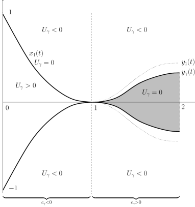
Figure 1: Fattening phenomenon for the functions $U_{\gamma}.$

Appendix: $L^{1}$-viscosity solutions and a stability result for weak convergence in time

We recall that the definition of $L^{1}$-viscosity solutions was introduced in Ishii’s paper [24]. We refer also to Nunziante [27, 28] and Bourgoing [11, 12] for a complete presentation of the theory.

Consider the equation

$$\left\{\begin{array}[]{l}\displaystyle{\frac{\partial v}{\partial t}={\bar{c}}(x,t)|Dv|\quad\mbox{in}\quad\mathbb{R}^{N}\times(0,T)}\\ \\ v(\cdot,0)=u_{0}\quad\mbox{in }\mathbb{R}^{N}\;,\end{array}\right.$$ (37)

where the velocity ${\bar{c}}:\mathbb{R}^{N}\times(0,T)\to\mathbb{R}$ is defined for almost every $t\in(0,T)$. We also assume that ${\bar{c}}$ satisfies
(H3) The function ${\bar{c}}$ is continuous with respect to $x\in\mathbb{R}^{N}$ and measurable in $t.$ For all $x,y\in\mathbb{R}^{N}$ and almost all $t\in[0,T],$

$$|{\bar{c}}(x,t)|\leq M\ \ \ {\rm and}\ \ \ |{\bar{c}}(x,t)-{\bar{c}}(y,t)|\leq L|x-y|.$$

Definition 4.1

($L^{1}$-viscosity solutions)
An upper-semicontinuous (respectively lower-semicontinuous) function $v$ on $\mathbb{R}^{N}\times[0,T]$ is a $L^{1}$-viscosity subsolution (respectively supersolution) of (37), if

$$v(0,\cdot)\leq u_{0}\quad(\mbox{respectively}\quad v(0,\cdot)\geq u_{0}),$$

and if for every $(x_{0},t_{0})\in\mathbb{R}^{N}\times[0,T]$, $b\in L^{1}(0,T)$, $\varphi\in C^{\infty}(\mathbb{R}^{N}\times(0,T))$ and continuous function $G:\mathbb{R}^{N}\times(0,T)\times\mathbb{R}^{N}\to\mathbb{R}$ such that
(i) the function

$$(x,t)\longmapsto v(x,t)-\int_{0}^{t}b(s)ds-\varphi(x,t)$$

has a local maximum (respectively minimum) at $(x_{0},t_{0})$ over $\mathbb{R}^{N}\times(0,T)$ and such that
(ii) for almost every $t\in(0,T)$ in some neighborhood of $t_{0}$ and for every $(x,p)$ in some neighborhood of $(x_{0},p_{0})$ with $p_{0}=D\varphi(x_{0},t_{0})$, we have

$${\bar{c}}(x,t)|p|-b(t)\leq G(x,t,p)\quad(\mbox{respectively}\quad{\bar{c}}(x,t)|p|-b(t)\geq G(x,t,p))$$

then

$$\frac{\partial\varphi}{\partial t}(x_{0},t_{0})\leq G(x_{0},t_{0},p_{0})\quad(\mbox{respectively}\quad\frac{\partial\varphi}{\partial t}(x_{0},t_{0})\geq G(x_{0},t_{0},p_{0})).$$

Finally we say that a locally bounded function $v$ defined on $\mathbb{R}^{N}\times[0,T]$ is a $L^{1}$-viscosity solution of (37), if its upper-semicontinuous (respectively lower-semicontinuous) envelope is a $L^{1}$-viscosity subsolution (respectively supersolution).

Theorem 4.2

(Existence and uniqueness in the $L^{1}$ sense)
For any $T>0$, under assumptions (H0) and (H3), there exists a unique $L^{1}$-viscosity solution to (37).

Finally, let us consider the solutions $v^{\varepsilon}$ to the following equation

$$\left\{\begin{array}[]{l}\displaystyle{\frac{\partial v^{\varepsilon}}{\partial t}={\bar{c}}^{\varepsilon}(x,t)|Dv^{\varepsilon}|\quad\mbox{in}\ \mathbb{R}^{N}\times(0,T)},\\[5.69054pt] v^{\varepsilon}(\cdot,0)=u_{0}\quad\mbox{in}\ \mathbb{R}^{N}\;.\end{array}\right.$$ (38)

The following stability result is a particular case of a general stability result proved by Barles in [6].

Theorem 4.3

($L^{1}$-stability) [6]
Under assumption (H0), let us assume that the velocity ${\bar{c}}^{\varepsilon}$ satisfies (H3) (with some constants $M,L$ independent of $\varepsilon$). Let us consider the $L^{1}$-viscosity solution $v^{\varepsilon}$ to (38). Assume that $v^{\varepsilon}$ converges locally uniformly to a function $v$ and, for all $x\in\mathbb{R}^{N},$

$$\hskip 14.22636pt\int_{0}^{t}{\bar{c}}^{\varepsilon}(x,s)ds\to\int_{0}^{t}{\bar{c}}(x,s)ds\ \ \ {locally\ uniformly\ in}\ (0,T).$$

Then $v$ is a $L^{1}$-viscosity solution of (37).

References

• [1] N. Alibaud. Existence, uniqueness and regularity for nonlinear degenerate parabolic equations with nonlocal terms. To appear in NoDEA Nonlinear Differential Equations Appl.
• [2] O. Alvarez, P. Cardaliaguet, and R. Monneau. Existence and uniqueness for dislocation dynamics with nonnegative velocity. Interfaces Free Bound., 7:415–434, 2005.
• [3] O. Alvarez, P. Hoch, Y. Le Bouar, and R. Monneau. Résolution en temps court d’une équation de Hamilton-Jacobi non locale décrivant la dynamique d’une dislocation. C. R. Math. Acad. Sci. Paris, 338(9):679–684, 2004.
• [4] O. Alvarez, P. Hoch, Y. Le Bouar, and R. Monneau. Dislocation dynamics: short-time existence and uniqueness of the solution. Arch. Ration. Mech. Anal., 181(3):449–504, 2006.
• [5] G. Barles. Solutions de viscosité des équations de Hamilton-Jacobi. Springer-Verlag, Paris, 1994.
• [6] G. Barles. A new stability result for viscosity solutions of nonlinear parabolic equations with weak convergence in time. C. R. Math. Acad. Sci. Paris, 343(3):173–178, 2006.
• [7] G. Barles, P. Cardaliaguet, O. Ley, and R. Monneau. Global existence results and uniqueness for dislocation equations. To appear in SIAM J. Math. Anal.
• [8] G. Barles, P. Cardaliaguet, O. Ley, and A. Monteillet. In preparation, 2007.
• [9] G. Barles and O. Ley. Nonlocal first-order Hamilton-Jacobi equations modelling dislocations dynamics. Comm. Partial Differential Equations, 31(8):1191–1208, 2006.
• [10] G. Barles, H. M. Soner, and P. E. Souganidis. Front propagation and phase field theory. SIAM J. Control Optim., 31(2):439–469, 1993.
• [11] M. Bourgoing. Vicosity solutions of fully nonlinear second order parabolic equations with ${L}^{1}$-time dependence and Neumann boundary conditions. To appear in NoDEA Nonlinear Differential Equations Appl.
• [12] M. Bourgoing. Vicosity solutions of fully nonlinear second order parabolic equations with ${L}^{1}$-time dependence and Neumann boundary conditions. existence and applications to the level-set approach. To appear in NoDEA Nonlinear Differential Equations Appl.
• [13] P. Cannarsa and H. Frankowska. Interior sphere property of attainable sets and time optimal control problems. ESAIM Control Optim. Calc. Var., 12(2):350–370 (electronic), 2006.
• [14] P. Cardaliaguet. On front propagation problems with nonlocal terms. Adv. Differential Equations, 5(1-3):213–268, 2000.
• [15] P. Cardaliaguet. Front propagation problems with nonlocal terms. II. J. Math. Anal. Appl., 260(2):572–601, 2001.
• [16] P. Cardaliaguet and C. Marchi. Regularity of the eikonal equation with Neumann boundary conditions in the plane: application to fronts with nonlocal terms. SIAM J. Control Optim., 45(3):1017–1038 (electronic), 2006.
• [17] Y. G. Chen, Y. Giga, and S. Goto. Uniqueness and existence of viscosity solutions of generalized mean curvature flow equations. J. Differential Geom., 33(3):749–786, 1991.
• [18] M. G. Crandall and P.-L. Lions. Viscosity solutions of Hamilton-Jacobi equations. Trans. Amer. Math. Soc., 277(1):1–42, 1983.
• [19] F. Da Lio, C. I. Kim, and D. Slepčev. Nonlocal front propagation problems in bounded domains with Neumann-type boundary conditions and applications. Asymptot. Anal., 37(3-4):257–292, 2004.
• [20] L. C. Evans and J. Spruck. Motion of level sets by mean curvature. I. J. Differential Geom., 33(3):635–681, 1991.
• [21] Y. Giga. Surface evolution equations, volume 99 of Monographs in Mathematics. Birkhäuser Verlag, Basel, 2006. A level set approach.
• [22] Y. Giga, S. Goto, and H. Ishii. Global existence of weak solutions for interface equations coupled with diffusion equations. SIAM J. Math. Anal., 23(4):821–835, 1992.
• [23] J. R. Hirth and L. Lothe. Theory of dislocations. Krieger, Malabar, Florida, second edition, 1992.
• [24] H. Ishii. Hamilton-Jacobi equations with discontinuous Hamiltonians on arbitrary open sets. Bull. Fac. Sci. Eng. Chuo Univ., 28:33–77, 1985.
• [25] O. Ley. Lower-bound gradient estimates for first-order Hamilton-Jacobi equations and applications to the regularity of propagating fronts. Adv. Differential Equations, 6(5):547–576, 2001.
• [26] F. R. N. Nabarro. Theory of crystal dislocations. Clarendon Press, Oxford, 1969.
• [27] D. Nunziante. Uniqueness of viscosity solutions of fully nonlinear second order parabolic equations with discontinuous time-dependence. Differential Integral Equations, 3(1):77–91, 1990.
• [28] D. Nunziante. Existence and uniqueness of unbounded viscosity solutions of parabolic equations with discontinuous time-dependence. Nonlinear Anal., 18(11):1033–1062, 1992.
• [29] S. Osher and J. Sethian. Fronts propagating with curvature dependent speed: algorithms based on Hamilton-Jacobi formulations. J. Comp. Physics, 79:12–49, 1988.
• [30] D. Rodney, Y. Le Bouar, and A. Finel. Phase field methods and dislocations. Acta Materialia, 51:17–30, 2003.
• [31] D. Slepčev. Approximation schemes for propagation of fronts with nonlocal velocities and Neumann boundary conditions. Nonlinear Anal., 52(1):79–115, 2003.
• [32] P. Soravia and P. E. Souganidis. Phase-field theory for FitzHugh-Nagumo-type systems. SIAM J. Math. Anal., 27(5):1341–1359, 1996.
• [33] A. Srour. Nonlocal second-order Hamilton-Jacobi equations arising in tomographic reconstruction. submitted, 2006.