Transmission through a defect in polyacene: the extreme limit of ultra narrow graphene

Abstract

We compute the transmission of an electron through an impurity in polyacene. For simplicity the disorder is confined to a single unit cell. When the impurity preserves the inversion symmetry around the central axis, the scattering problem can be reduced to that of two independent chains with an alternating sequence of two types of atoms. An analytical expression for the transmission coefficient is derived. On-site and off-diagonal defects are considered and shown to display very different electron scattering properties.

1 Introduction

The study of polyacene started long ago in a pioneering paper by Kivelson and Chapman.[1] The study performed by these two authors was motivated by the investigations of Su, Schreiffer, and Heeger on polyacetylene.[2, 3] They[1] showed that the band structure associated to the $\pi$-orbitals of polyacene is made of four bands, with a valence and a conduction bands touching at the limit of the one-dimensional Brillouin zone. Since polyacene can be considered the extreme case of a narrow graphene[4, 5] ribbon it is instructive to compare the band structure of graphene and polyacene. In both cases one has an electron per carbon atom and in both cases the valence and conduction band touch at the corner of the Brillouin zone. In graphene, however, the bands are linear at the $\bm{K}$ and $\bm{K}^{\prime}$ points of the Brillouin zone, whereas in polyacene the dispersion relation around the momentum $k=\pi/a$ ($a$ the length of the unit cell) is quadratic. As a consequence, graphene has a vanishing density of states at the Fermi energy whereas polyacene displays a square root singularity. It was therefore speculated[1] that the ground state of polyacene could support long range order such as ferromagnetic and superconducting phases. It was further showed that phonon modes in polyacene can lead to a Peierls distortion opening an energy gap at $k=\pi/a$. [1, 6]

Using a Green’s function method, Rosa and Melo[7] studied the density of states of several distorted configurations of polyacene, including the case where a local defect was present. They found that the optical response of polyacene should be very different from that of polyacetylene. The inclusion of many-body effects on the description of the ground state of polyacene was done by Garcia-Bach et al.[8] using a valence-bond treatment. They found that the distorted ground state is degenerate. Using a projector quantum Monte Carlo method, Srinivasan and Ramasesha [9] found, within the Hubbard model, that electron-electron correlations tend to enhance the Peierls instability. With the development of the density matrix renormalization group, the exact study of the ground state of quasi-one-dimensional electronic systems became available. Raghu et al.[10] studied the ground state of polyacene using the Pariser-Parr-Pople Hamiltonian. As in previous studies they found that strong electron-electron interactions can enhance the dimerization. Using a configuration interaction technique, Sony and Shukla [11] studied the optical absorption and the excited states of polyacenes also in the framework of the Pariser-Parr-Pople Hamiltonian.

As interesting as the ground state nature of carbon polymers are their transport properties. Of particular interest to us is the effect of disorder on the electronic tunneling through a portion of a disordered chain. Guinea and Vergés, [12] using a Green’s function method, studied the local density of states and the localization length of a one-dimensional chain coupled to small pieces of laterally linked polymer. They showed that at the band center there is an exact vanishing of the transmission coefficient due to a local antiresonance. Sautet and Joachim [13] studied, within a one-dimensional tight-binding model, the effect of a single impurity which would change both the on-site energy and the hopping to the next-neighbor atoms. Mizes and Conwell [14] consider the effect of a single impurity in the square polymer, showing that a change on the on-site energy has a more pronounced effect in reducing the transmission in the one-dimensional chain than in the square polymer. At the end of the paper[14] these authors speculate that for polyacene there should be four active scattering modes instead of two as in the square polymer. As we show in this paper, this is not the case because the band structure of polyacene is markedly different from that of the square polymer. Gu et al. [15] generalized the study of Ref. [14] by including different types of obstacles as scattering centers. Yu el al. [16] studied the electronic transmission through a conjugate-oligomer using both mode matching and Green’s function methods. They found that the transmission through the conjugate-oligomer possesses several transmission resonances. Farchioni et al.[17] studied the transport properties of emeraldine slats using a Green’s function method, by looking at the effect on the electronic transmission of impurity dimers. The band structure of very narrow carbon nanoribbons was studied by Ezawa. [18] The effect on the conductance of the parity of the number of carbon rows across a zig-zag ribbon has been studied by Akhmerov et al..[19]

In this paper we study the effect of disorder on the electronic transmission in polyacene. This system can be considered the most extreme limit of narrow carbon nanoribbons,[18] and it corresponds to an odd parity situation studied in Ref. [19]. We shall assume that the disorder is limited to a single unit cell. Although this assumption can be relaxed, it allows us however to obtain a full analytical expression for the transmission coefficient. Following Ref. [13] we shall consider both on-site and hopping disorder. The system is therefore characterized by two semi-infinite perfect leads made of polyacene and a scattering region. The Schrödinger equation has to be solved for the three regions and a mode matching technique, first used by Ando [20] to study the conductance of a square lattice in a magnetic field, will be used here. Although, as discussed above, all the theoretical studies point out that polyacene has a gap at the Fermi energy due to phonons and interactions, here we will consider non-distorted polyacene in the independent particle approximation. It should be relatively simple to generalize the calculations below to include the effect of a gap and the effect of electron-electron interactions (at least at the mean field level), but the only expected modification would be a small region near zero energy where the conductance would be zero due to the presence of the gap. In addition, the disorder could add states into the gap of polyacene.

2 Model for disordered polyacene

The model for disordered polyacene can be written in general terms as

$$H = \sum_{n=-\infty}^{\infty}\sum_{i,j=1}^{4}[\delta_{ij}\epsilon(n,i)|n,i\rangle\langle n,j|$$ (1)

$$+ t_{\rm intra}(n,i,j)|n,i\rangle\langle n,j|$$

$$+ t_{\rm inter}(n,i,j)|n,i\rangle\langle n+1,j|]\,,$$

where $\epsilon(n,i)$ represents the on-site energy, $t_{\rm intra}(n,i,j)$ the hopping between the atoms within the unit cell $n$, and $t_{\rm inter}(n,i,j)$ the hopping between atoms in neighboring unit cells. The sum over $n$ runs over the unit cells and the sums over $i$ and $j$ run over the atoms in the unit cell. In our model we shall assume that the on-site energies $\epsilon(0,1)=\epsilon_{0}$ and $\epsilon(0,4)=\epsilon_{0}$ are different from those of the rest of the atoms in the lattice. The on-site energies for atoms to the left of these two are all equal to $\epsilon_{L}$ and, for those to the right, to $\epsilon_{R}$. This difference could be due to a potential bias applied to the system. The hopping parameters are defined in Figs. 1 and 2. Only the hopping energies starting at the atoms 1 and 4 of the zero unit cell are modified. They are named $t_{L}$ and $t_{R}$. We further assume that the hopping energies between atoms 2 and 3 within a given unit cell ($t_{\perp}$) can be different from that between atoms 1 and 2, or 3 and 4 ($t$). The eigenfunctions of this problem have the form

$$|\Psi\rangle=\sum_{n}\sum_{j}c(n,j)|n,j\rangle.$$ (2)

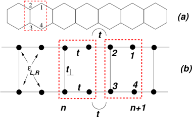
Figure 1: (color online) Representation of polyacene in (a) and its topologically equivalent lattice in (b). Each unit cell has four atoms. The on-site energy is $\epsilon_{L,R}$. The hoping along the chain is $t$ and in the perpendicular direction is $t_{\perp}$.

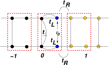
Figure 2: (color online) Characterization of the $n=0$ unit cell, where the disorder is located. Note that the on-site energies for $n<0$ ($\varepsilon_{L}$) are different from those for $n>0$ ($\varepsilon_{R}$). Also the on-site energy of atoms 1 and 4 in the zero unit cell is different from the rest and equals $\epsilon_{0}$.

As it is clear from Fig 2 the problem is divided into three regions: (i) that to the left of the zero unit cell, with $n=-\infty,\ldots,-1$, representing a semi-infinite ordered lead; (ii) the disordered unit cell at $n=0$, which will induce the scattering of the electrons; (iii) the right ordered lead, for $n=1,\ldots,\infty$. We have therefore to solve the problem in these three regions. The method we will use was developed by Ando[20] in the context of quantum point contacts in a magnetic field and generalized by Khomyakov et al. [21] to an arbitrary three-dimensional structure.

The strategy of solution is therefore the following, firstly the problem is solved for the pure leads obtaining the eigenmodes. Then the scattering problem is solved considering an incoming wave described by one of the eigenmodes at a time. This allows for the determination of the transmission matrix elements $t_{\mu\nu}$, and from them the calculation of the conductance follows as [22, 23]

$$G=\frac{2e^{2}}{h}\sum_{\mu\nu}|t_{\mu\nu}|^{2}\,,$$ (3)

where the summation is over propagating channels only.

3 Solution of the scattering problem

As explained above, the problem is separated into the solution in the perfect leads and the solution in the scattering region. In what follows we shall explain how to obtain those solutions.

3.1 Scattering channels

We study here the scattering channels, i.e. stationary solutions in the asympotic leads assuming these are perfect and infinite. Let us start with the left lead. The problem for the right one is solved along the same lines but with $\epsilon_{L}$ replaced by $\epsilon_{R}$. The tight-binding Hamiltonian for $m=-\infty,\ldots,-2$ has the form

$$-\bm{B}\bm{c}_{m-1}+(\bm{I}E-\bm{H}_{L})\bm{c}_{m}-\bm{B}^{\dagger}\bm{c}_{m+1}=0\,,$$ (4)

where $\bm{c}_{m}$ is a 4-vector containing the wave-function coefficients of the unit cell $m$. The matrices $\bm{B}$ and $\bm{H}_{L}$ are given by

$$\bm{B}=\left(\begin{array}[]{cccc}0&0&0&0\\ t&0&0&0\\ 0&0&0&t\\ 0&0&0&0\end{array}\right)\,,$$ (5)

and

$$\bm{H}_{L}=\left(\begin{array}[]{cccc}\epsilon_{L}&t&0&0\\ t&\epsilon_{L}&t_{\perp}&0\\ 0&t_{\perp}&\epsilon_{L}&t\\ 0&0&t&\epsilon_{L}\end{array}\right)\,.$$ (6)

It is important to note that the $\bm{B}$ matrix is singular, not having an inverse. This will be important in what follows. As explained by Ando, [20] the problem for the perfect lead may be solved assuming a Bloch relation between the vectors $\bm{c}_{m}$

$$\bm{c}_{m+1}=\lambda\bm{c}_{m}\,.$$ (7)

For a general problem the vector $\bm{c}_{m}$ has dimension $M$ and the solution of (4) can be obtained by transforming it into an ordinary eigenvalue equation of dimension $2M$.[20] We look for scattering states formed by an incoming wave approaching the scattering region from the left and its resulting outgoing waves. Whether these waves are propagating or evanescent states depends on the nature of the eigenvalues. Propagating states always have $|\lambda|=1$, whereas evanescent ones have $|\lambda|\neq 1$. Another possibility is to transform Eq. (4) into a quadratic eigenvalue equation by repeatedly use of Eq. (7), resulting in

$$-\bm{B}\bm{c}_{m}+(\bm{I}E-\bm{H}_{L})\lambda\bm{c}_{m}-\bm{B}^{\dagger}\lambda^{2}\bm{c}_{m}=0\,.$$ (8)

As before, the determination of the eigenvalues of Eq. (8) will lead, for a problem of dimension $M$, to a polynomial of order $2M$ whose roots are the sought eigenvalues.

Although we can attack the solution of the problem (8) using the matrices given by Eqs. (5) and (6), it is however convenient to perform a unitary transformation of Eq. (8). We define the unitary matrix $\bm{U}$

$$\bm{U}=\frac{1}{\sqrt{2}}\left(\begin{array}[]{cccc}1&0&0&1\\ 0&1&1&0\\ 1&0&0&-1\\ 0&1&-1&0\end{array}\right)\,,$$ (9)

and introduce the transformation $\bm{\tilde{c}}_{m}=\bm{U}\bm{c}_{m}$, and $\bm{\tilde{M}}=\bm{U}\bm{M}\bm{U}^{-1}$. Upon this transformation, the eigenproblem (8) is reduced to two block-diagonal quadratic eigenvalue problems, since the resulting transforms of $\bm{B}$ and $\bm{H}_{L}$ are factorized into two $2\times 2$ matrices which we denote generally as $\bm{b}$ and $\bm{h}_{L}$. Correspondingly, $\bm{\tilde{c}}_{m}$ becomes the direct sum of two 2-vectors which we generically refer to as $\bm{u}_{m}$ and which we assume normalized. The resulting eigenvalue problem reads

$$-\bm{b}\bm{u}_{m}+\lambda(\bm{I}E-\bm{h}_{L})\bm{u}_{m}-\lambda^{2}\bm{b}^{\dagger}\bm{u}_{m}=0\,,$$ (10)

with

$$\bm{b}=\left(\begin{array}[]{cc}0&0\\ t&0\end{array}\right)$$ (11)

and

$$\bm{h}_{L}=\left(\begin{array}[]{cc}\epsilon_{L}&t\\ t&\epsilon_{L}\pm t_{\perp}\end{array}\right)\,.$$ (12)

The decoupled two-dimensional problems describe propagation through the even and odd modes with respect to the central axis of the polyacene. The eigenvalue problem (10) has the same form as that of a linear chain, with hopping energy $t$ between neighboring atoms and with on-site energies alternating between $\epsilon_{L}$ and $\epsilon_{L}\pm t_{\perp}$. As a conclusion, the scattering problem in polyacene can be mapped into that of two independent one-dimensional chains, contrary to the expectations of Mizes and Conwell. [14]

From the general discussion above one would expect that the eigenvalue problem (10) would lead to a quartic polynomial in $\lambda$. In fact because the matrix $\bm{B}$ has no inverse (as happens for $\bm{b}$) the polynomial is only cubic in $\lambda$. One of the solutions is the trivial one $\lambda=0$. This solution has to be disregarded since it would produce a null wave function everywhere. The other two solutions are

$$\lambda = [(E-\epsilon_{L})^{2}+t_{\perp}(E-\epsilon_{L})-2t^{2}]/2t^{2}$$ (13)

$$\pm \frac{1}{2}\sqrt{[(E-\epsilon_{L})^{2}+t_{\perp}(E-\epsilon_{L})-2t^{2}]^{2}/t^{4}-4}\,.$$

When the square root becomes imaginary, Eq. (13) gives the momentum of a propagating Bloch wave. If we now consider the case $t_{\perp}\rightarrow-t_{\perp}$ [see Eq. (12)] two other solutions are obtained.

The fact that we only have two solutions for each sign of $t_{\perp}$, and not four, means that there are always two of the four expected modes that do not contribute to the transport, not even as evanescent waves. This result could have been anticipated if we had considered the energy bands of perfect polyacene. [1] These are given by

$$E-\epsilon_{L}=\pm\frac{t_{\perp}}{2}\pm\frac{1}{2}\sqrt{t_{\perp}^{2}+8t^{2}[1+\cos(ka)]}\,,$$ (14)

where $a$ is the length of the unit cell and $k\in[-\pi/a,\pi/a]$. If we now try to solve for $k$ in Eq. (14) one finds that for a given energy $E$ only two bands give a solution, being it real or complex.

The velocity of the electrons in the modes is given by [21]

$$v=-\frac{2a}{\hbar}\Im[\lambda\bm{u}^{\dagger}\bm{b}^{\dagger}\bm{u}]\,.$$ (15)

For the present problem the velocity has a simple form given by

$$v=-\frac{2at}{\hbar}\Im[\lambda u_{A}u_{B}]\,,$$ (16)

where $u_{A}$ and $u_{B}$ are the components of $\bm{u}_{m}$, orbital $A$ resulting from the (symmetric or antisymmetric) linear combination of sites 2 and 3 within the cell and orbital $B$ stemming from the similar combination of sites 1 and 4 (see Fig. 1). These amplitudes are given by

$$u_{A}=\frac{t|1+\lambda|}{\sqrt{(E-\epsilon_{L})^{2}+t^{2}|1+\lambda|^{2}}}\,,$$ (17)

and

$$u_{B}=\frac{(1+\lambda^{\ast})(E-\epsilon_{L})}{|1+\lambda|\sqrt{(E-\epsilon_{L})^{2}+t^{2}|1+\lambda|^{2}}}\,.$$ (18)

Using Eqs. (17) and (18) the velocity (16) reads

$$v=-\frac{2at}{\hbar}\frac{t(E-\epsilon_{L})}{(E-\epsilon_{L})^{2}+t^{2}|1+\lambda|^{2}}\Im\lambda\,.$$ (19)

Equation (19) allows to identify the right and left moving modes for a given energy $E$. The right lead is solved in the same way with $\epsilon_{L}$ replaced by $\epsilon_{R}$.

3.2 The scattering region

We now want to describe the scattering region. The Schrödinger equation for the unit cell $m=-1$ has the same form as before, except that it couples to $\bm{c}_{0}$. For the unit cell $m=0$ the Schrödinger equation is written as

$$-\bm{B}\bm{c}_{-1}+(\bm{I}E-\bm{H}_{00})\bm{c}_{0}-\bm{B}^{\dagger}_{R}\bm{c}_{1}=0\,$$ (20)

with the matrices $\bm{H}_{00}$ and $\bm{B}_{R}$ given by

$$\bm{H}_{00}=\left(\begin{array}[]{cccc}\epsilon_{0}&t_{L}&0&0\\ t_{L}&\epsilon_{L}&t_{\perp}&0\\ 0&t_{\perp}&\epsilon_{L}&t_{L}\\ 0&0&t_{L}&\epsilon_{0}\end{array}\right)\,,$$ (21)

and

$$\bm{B}_{R}=\left(\begin{array}[]{cccc}0&0&0&0\\ t_{R}&0&0&0\\ 0&0&0&t_{R}\\ 0&0&0&0\end{array}\right)\,.$$ (22)

For the unit cell $m=1$ the Schrödinger equation has the same form as Eq. (4) except that $\bm{B}$ is replaced by $\bm{B}_{R}$, $\epsilon_{L}$ is replaced by $\epsilon_{R}$ and it couples to $\bm{c}_{0}$. As before we can perform a unitary transformation of the Schrödinger equation leading to an effective $2\times 2$ Hamiltonian. The Hamiltonian for unit cell $m=-1$ has the same form as Eq. (10). For the unit cell $m=0$ we obtain

$$-\bm{b}\bm{u}_{-1}+(\bm{I}E-\bm{h}_{00}){\bm{u}_{0}}-\bm{b}_{R}^{\dagger}\bm{u}_{1}=0\,,$$ (23)

and for $m=1$

$$-\bm{b}_{R}\bm{u}_{0}+(\bm{I}E-\bm{h}_{R}){\bm{u}_{1}}-\bm{b}^{\dagger}\bm{u}_{2}=0\,.$$ (24)

The matrix $\bm{b}_{R}$ has the same form as $\bm{b}$ with $t$ replaced by $t_{R}$. The matrix $\bm{h}_{R}$ is obtained from $\bm{h}_{L}$ replacing $\epsilon_{L}$ by $\epsilon_{R}$. The matrix $\bm{h}_{00}$ is given by

$$\bm{h}_{00}=\left(\begin{array}[]{cc}\epsilon_{0}&t_{L}\\ t_{L}&\epsilon_{L}\pm t_{\perp}\end{array}\right)\,.$$ (25)

Since the full problem factorizes into two block-diagonal problems and, furthermore, because in the leads, for each $2\times 2$ block, only one mode is active, the scattering takes place without mode mixing. This is a considerable simplification over the general approach of Refs. [20, 21].

If we define $\bm{u}^{\pm}_{m}$ as the amplitude at cell $m$ of the Bloch wave propagating to the right ($+$) or left ($-$) in perfect polyacene, the following relation holds:

$$\bm{u}^{\pm}_{-m+1}=\lambda^{\pm}\bm{u}^{\pm}_{-m}\,,$$ (26)

where $\lambda^{\pm}=1/\lambda^{\mp}$ is given in Eq. (13) for the asympotic left lead. Using Eq. (26) we can write

$$\bm{u}_{-2}=\left(\lambda^{-}-\lambda^{+}\right)\bm{u}^{+}_{-1}+\lambda^{+}\bm{u}_{-1}\,.$$ (27)

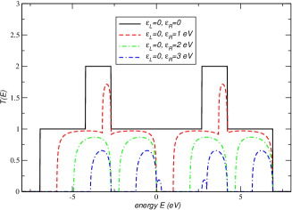
Figure 3: (color on line) Representation of the transmission $T(E)$ for different values of $\epsilon_{R}$. The parameters are $t=t_{\perp}=t_{L}=t_{R}=-2.7$ eV, $\epsilon_{0}=\epsilon_{L}=0$. The solid line corresponds to perfect polyacene.

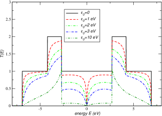
Figure 4: (color on line) Representation of the transmission $T(E)$ for different values of $\epsilon_{0}$. The parameters are $t=t_{\perp}=t_{L}=t_{R}=-2.7$ eV, $\epsilon_{L}=\epsilon_{R}=0$. The solid line corresponds to perfect polyacene.

The boundary conditions require the specification of $\bm{u}^{+}_{-1}$, which will represent an incoming wave function in one of the modes of the left lead. On the right lead we have only a scattered wave propagating to the right, we thus write

$$\bm{u}_{2}=\lambda^{+}\bm{u}_{1}\,.$$ (28)

Using Eqs. (27) and (28), the determination of the wave function on the unit cells $m=-1,0,1$ reduces to the resolution of the following system of linear equations

$$[\bm{I}E-\bm{h}_{L}-\lambda^{+}\bm{b}]\bm{u}_{-1}-\bm{b}^{\dagger}\bm{u}_{0}=(\lambda^{-}-\lambda^{+})\bm{u}^{+}_{-1}\,,$$ (29)

$$-\bm{b}\bm{u}_{-1}+(\bm{I}E-\bm{h}_{00}){\bm{u}_{0}}-\bm{b}^{\dagger}_{R}\bm{u}_{1}=0\,,$$ (30)

$$-\bm{b}_{R}\bm{u}_{0}+(\bm{I}E-\bm{h}_{R}-\bm{b}^{\dagger}\lambda^{+})\bm{u}_{1}=0\,.$$ (31)

Once the system is solved the vector $\bm{u}_{1}$ is determined. We can then write $\bm{u}_{1}$ as

$$\bm{u}_{1}=\bm{u}^{+}_{1}\tau_{\alpha}\,,$$ (32)

where $\alpha$ is an explicit index to label the (odd or even) mode. The physical transmission matrix element is given by[23]

$$t_{\alpha}=\sqrt{\frac{v_{R}}{v_{L}}}\tau_{\alpha}\,,$$ (33)

where $v_{L/R}$ represents the velocity of the considered mode in the left/right lead, given by Eq. (19). The total conductance is obtained by summing the contributions from the symmetric and the antisymmetric mode,

$$G=\frac{2e^{2}}{h}T(E)=\frac{2e^{2}}{h}\sum_{\alpha=1}^{2}|t_{\alpha}|^{2}\,,$$ (34)

assuming that both modes are propagating waves. Solving explicitly the linear system of equations defined above, the expression for $\tau_{\alpha}$ is obtained,

$$\tau_{\alpha}=qt^{3}t_{L}t_{R}u^{+}_{A}\lambda^{-}\frac{\eta}{D}\,,$$ (35)

where

$$q=\lambda^{-}-\lambda^{+}\,,$$ (36)

$$\eta=\frac{E-\epsilon_{R}}{u_{B}^{+}}\,,$$ (37)

and $u^{+}_{A},u^{+}_{B}$ are the $m$-independent parts of the $A$ and $B$ components of $\bm{u}_{m}^{+}$ in the left and right leads, respectively. The denominator $D$ reads

$$D = -t^{2}_{L}[t^{2}+(t^{2}-E(E+t_{\perp})+\epsilon_{L}(2E+t_{\perp}-\epsilon_{L}))\lambda^{-}_{L}]$$ (38)

$$\times [t^{2}-E(E+t_{\perp})+\epsilon_{R}(2E+t_{\perp}-\epsilon_{R})+t^{2}\lambda^{+}_{R}]$$

$$+ (E+t_{\perp}-\epsilon_{L})[-t^{2}+(-2t^{2}+E(E+t_{\perp})-\epsilon_{L}(2E+t_{\perp}-\epsilon_{L}))\lambda^{-}_{L}]$$

$$\times [t^{2}_{R}(-E+\epsilon_{R})+(E-\epsilon_{0})(-t^{2}+E(E+t_{\perp})-\epsilon_{R}(2E+t_{\perp}-\epsilon_{R})-t^{2}\lambda^{+}_{R})]\,.$$

We are now in position to study the transmission coefficient $T(E)$. In Figure 3 we study the transmission of the electrons in a situation that mimics that of a potential step in ordinary quantum mechanics problems. The potential barrier is created by having the sites at the right of the unit cell $n=0$ at a different energy from those at the left. For definiteness we consider $\epsilon_{L}=0$. When $\epsilon_{L}=\epsilon_{R}$, $T(E)$ has a step structure, represented by the solid line in Fig. 3, due to the existence of two possible conducting channels. These two conducting channels are those associated with the two effective one-dimensional chains. For energies where the two channels of the two chains are propagating states, one obtains $T(E)=2$; when only one channel is active one obtains $T(E)=1$. Having now $\epsilon_{L}\neq\epsilon_{R}$ induces some back scattering of the electrons at the interface, reducing the value of $T(E)$. When the difference between $\epsilon_{L}$ and $\epsilon_{R}$ increases we see the appearance of zones of zero transmission, while this is always nonzero for $\epsilon_{L}=\epsilon_{R}$.

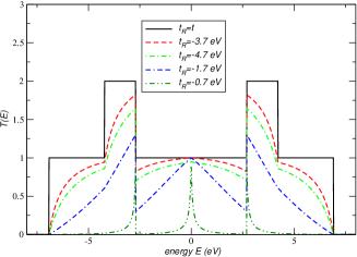
Figure 5: (color on line) Representation of the transmission $T(E)$ for different values of the hopping $t_{R}$ and $t_{L}$. The parameters are $t=t_{\perp}=-2.7$ eV, $\epsilon_{L}=\epsilon_{R}=\epsilon_{0}=0$, $t_{R}=t_{L}$. The solid line corresponds to perfect polyacene.

In Figure 4 we study the effect of changing the value of $\epsilon_{0}$ relatively to that of $\epsilon_{L}$ and $\epsilon_{R}$. Overall there is an effect of diminishing $T(E)$. If the difference between $\epsilon_{0}$ and $\epsilon_{L}$ and $\epsilon_{R}$ is not very large the $T(E)$ curve follows closely that for the non-disordered case. There is however an exception at zero energy, where $T(E)$ tends to zero, leading to a totally reflecting barrier. This can be due to a local antiresonance as in Refs. [12, 24].

On the contrary, if the disorder is induced by changing the hopping, the behavior of $T(E)$ shows almost perfect transmission at $E=0$, as can be seen in Fig. 5. This effect is particularly clear when $t_{L}$ and $t_{R}$, become very small. From Eq. (35) we see that $T(E)$ will vanish as the fourth power of $t_{L}$ ($t_{L}=t_{R}$); nevertheless close to $E=0$ the system has a strong enhancement of its transmission. Away from this special point the curves for $T(E)$ are similar to those of Fig. 4 for on-site disorder.

In the cases of Figs. 4 and 5 the conductance of the system would exhibit conductance oscillations as long as the scattering strength of the defect is not too strong.

4 Conclusions

In this paper we have studied analytically the electronic transmission of polyacene due to on-site and off-diagonal disorder. We have shown that the system is equivalent to two decoupled linear chains of atoms, with alternating on-site energies and a constant hopping parameter. Scattering occurs in the system without mode mixing if inversion symmetry around the central axis is preserved. We find that on-site and hopping disorder have markedly distinct scattering properties close to zero energy. Whereas for on-site disorder the transmission decreases strongly close to zero energy, for hopping disorder the transmission is enhanced. If the system opens up a gap at the Fermi energy, we expect these same characteristics to occur near the gap edge.

References

- [1] S. Kivelson and O. L. Chapman, Phys. Rev. B 28, 7236 (1983).
- [2] W. P. Su, J. R. Schreiffer, and A. J. Heeger, Phys. Rev. Lett. 42, 1698 (1979).
- [3] W. P. Su, J. R. Schreiffer, and A. J. Heeger, Phys. Rev. B 22, 2099 (1980); 28, 1138(E) (1983).
- [4] K. S. Novoselov, A. K. Geim, S. V. Morozov, D. Jiang, Y. Zhang, S. V. Dubonos, I. V. Grigorieva, and A. A. Firsov, Science 306, 666 (2004).
- [5] K. S. Novoselov, D. Jiang, T. Booth, V. V. Khotkevich, S. M. Morozov, A. K. Geim, PNAS 102, 10451 (2005).
- [6] I. Bozovic, Phys. Rev. B 32 8136 (1985).
- [7] A. L. S. Rosa and C. P. de Melo, Phys. Rev. B 38, 5430 (1988).
- [8] M. A. Garcia-Bach, A. Penaranda, and D. J. Klein, Phys. Rev. B 45, 10891 (1992).
- [9] B. Srinivasan and S. Ramasesha, Phys. Rev. B 57, 8927 (1998).
- [10] C. Raghu, Y. Anusooya Pati, and S. Ramasesha, Phys. Rev. B 65, 155204 (2002).
- [11] P. Sony and A. Shukla, Phys. Rev. B 75, 155208 (2007).
- [12] F. Guinea and J. A. Vergés, Phys. Rev. B 35, 979 (1987).
- [13] P. Sautet and C. Joachim, Phys. Rev. B 38, 12238 (1988).
- [14] H. Mizes and E. Conwell, Phys. Rev. B 44, 3963 (1991).
- [15] Ben-yuan Gu, Chong-ru Huo, Zi-zhao Gan, Guo-zhen Yang, and Jian-qing Wang, Phys. Rev. B 46, 13274 (1992).
- [16] Z. G. Yu, L. Smith, A. Saxena, and A. R. Bishop, Phys. Rev. B 56 6494 (1997); Phys. Rev. B 59 16001 (1999).
- [17] R. Farchioni, P. Vignolo, and G. Grosso Phys. Rev. B 60, 15705 (1999)
- [18] M. Ezawa, Phys. Rev. B 73, 045432 (2006).
- [19] A. R. Akhmerov, J. H. Bardarson, A. Rycerz, and C. W. J. Beenakker, arXiv:0712.3233.
- [20] T. Ando, Phys. Rev. B 44, 8017 (1991).
- [21] P. A. Khomyakov, G. Brocks, V. Karpan, M. Zwierzycki, and P. J. Kelly Phys. Rev. B 72, 35450 (2005).
- [22] M. Buttiker, Y. Imry, R. Landauer, S. Pinhas, Phys. Rev. B 31, 6207 (1985).
- [23] S. Datta, Electronic Transport in Mesoscopic Systems, (Cambridge University Press, Cambridge, 1995).
- [24] F. Sols, M. Macucci, U. Ravaioli, and K. Hess, J. Appl. Phys. 66, 3892 (1989).