Pion Compton scattering and bremsstrahlung

Abstract

The pion-polarizability functions are structure functions of pion-Compton scattering. They can be assessed in high-energy pion-nucleus bremsstrahlung reactions, $\pi^{-}+A\rightarrow\pi^{-}+\gamma+A$. We present numerical expectations for pion-nucleus bremsstrahlung cross sections in the Coulomb region, i.e. the small-angle region where the nuclear scattering is dominated by the Coulomb interaction. We investigate the prospects of measuring the polarizability functions for pion-Compton c.m. energies from threshold up to 1 GeV. A meson-exchange model is used for the pion-Compton amplitude.

I Introduction

The cross-section distribution for high-energy pionic bremsstrahlung

$$\pi^{-}+A\rightarrow\pi^{-}+\gamma+A,$$

is at small-momentum transfers to the nucleus dominated by the one-photon-exchange contribution. Hence, by measuring cross-section distributions for pion-nucleus bremsstrahlung at small momentum transfers one gains at the same time information about the cross-section distribution for pion-Compton scattering

$$\gamma+\pi^{-}\rightarrow\gamma+\pi^{-};$$

the photon of the initial state being the virtual photon exchanged between pion and nucleus. In particular, it becomes possible to determine pion polarizabilities.

The theoretical underpinnings of the pion-bremsstrahlung reaction were investigated by Gal’perin et al. 4 , and an experiment was susequently performed by Antipov et al. Ant , which showed that pion polarizabilities could indeed be determined. The COMPASS experiment at CERN COMP is a refinement of the Antipov experiment.

In ref.FT a mathematical expression for the bremsstrahlung cross section was derived assuming a pion-Compton amplitude that in additon to the Born contributions contained also contributions from the $\sigma$, $\rho$, and $a_{1}$, exchanges. The kinematics of the nuclear reaction was defined through

$$\pi^{-}(p_{1})+{\rm A}(p)\rightarrow\pi^{-}(p_{2})+\gamma(q_{2})+{\rm}A(p^{\prime}),$$ (1)

and the kinematics of the related pion-Compton reaction through

$$\pi^{-}(p_{1})+\gamma(q_{1})\rightarrow\pi^{-}(p_{2})+\gamma(q_{2}),$$ (2)

with $q_{1}=p-p^{\prime}$. In terms of these kinematic variables the cross-section distribution can be written as FT

$$\frac{\textrm{d}\sigma}{\textrm{d}^{2}q_{1\bot}\textrm{d}^{2}q_{2\bot}\textrm{d}x} = \frac{4Z^{2}\alpha^{3}}{\pi^{2}m_{\pi}^{4}}\Bigg{[}\frac{\mbox{\boldmath{${q}$}}_{1\bot}^{2}}{(\mbox{\boldmath{${q}$}}_{1\bot}^{2}+q_{min}^{2})^{2}}\Bigg{]}\Bigg{[}\frac{1-x}{x^{3}}\Bigg{]}\Bigg{[}\left(\frac{x^{2}m_{\pi}^{2}}{\mathbf{q}_{2\bot}^{2}+x^{2}m_{\pi}^{2}}\right)^{2}\Bigg{]}\cdot$$ (3)

$$\Bigg{[}\left|A(x,\mathbf{q}_{2\bot}^{2})\right|^{2}\left\{1-\mu^{2}\frac{4x^{2}m_{\pi}^{2}\mathbf{q}_{2\bot}^{2}}{(x^{2}m_{\pi}^{2}+\mathbf{q}_{2\bot}^{2})^{2}}\right\}$$

$$\qquad+2\Re\left(A(x,\mathbf{q}_{2\bot}^{2})B^{\star}(x,\mathbf{q}_{2\bot}^{2})\right)\left\{1-\mu^{2}\frac{2\mathbf{q}_{2\bot}^{2}}{x^{2}m_{\pi}^{2}+\mathbf{q}_{2\bot}^{2}}\right\}$$

$$\qquad+\left|B(x,\mathbf{q}_{2\bot}^{2})\right|^{2}\Bigg{]}.$$

This expression is valid when the transverse momenta of the emerging pion and photon are much smaller than their longitudinal momenta. The parameter $\alpha$ is the fine-structure constant, $m_{\pi}$ the pion mass, $x$ the ratio

$$x=\frac{q_{2z}}{p_{1}}=\frac{\omega_{2}}{E_{1}},$$ (4)

$\mu=\hat{\mathbf{q}}_{1\bot}\cdot\hat{\mathbf{q}}_{2\bot}$, and $q_{min}$ the minimum-longitudinal-momentum transfer

$$q_{min}=\frac{m_{\pi}^{2}}{2E_{1}}\cdot\frac{x}{1-x}.$$ (5)

At high energies $q_{min}$ is extremely small.

The functions $A(x,\mathbf{q}_{2\bot}^{2})$ and $B(x,\mathbf{q}_{2\bot}^{2})$ characterize the pion-Compton amplitude. In the Born approximation

$$A(x,\mathbf{q}_{2\bot}^{2})=1,$$ (6)

$$B(x,\mathbf{q}_{2\bot}^{2})=0;$$ (7)

and generally

$$A(x,\mathbf{q}_{2\bot}^{2}) = 1-\frac{x^{2}}{4(1-x)}\left(\frac{\mathbf{q}_{2\bot}^{2}+x^{2}m_{\pi}^{2}}{x^{2}m_{\pi}^{2}}\right)^{2}\lambda_{1}(x,\mathbf{q}_{2\bot}^{2}),$$ (8)

$$B(x,\mathbf{q}_{2\bot}^{2}) = \frac{x^{2}}{2(1-x)}\left(\frac{\mathbf{q}_{2\bot}^{2}+x^{2}m_{\pi}^{2}}{x^{2}m_{\pi}^{2}}\right)\lambda_{2}(x,\mathbf{q}_{2\bot}^{2}),$$ (9)

with $\lambda_{1}(x,\mathbf{q}_{2\bot}^{2})$ and $\lambda_{2}(x,\mathbf{q}_{2\bot}^{2})$ generalized-polarizability functions. Their mathematical expressions, in the meson-exchange model, are given in FT .

The structure of the cross-section distribution is mainly determined by the inelastic-Coulomb factor

$$\frac{\mbox{\boldmath{${q}$}}_{1\bot}^{2}}{(\mbox{\boldmath{${q}$}}_{1\bot}^{2}+q_{min}^{2})^{2}}$$ (10)

which vanishes when the transverse-momentum transfer $\mbox{\boldmath{${q}$}}_{1\bot}$ to the nucleus vanishes. This is the classic Primakoff factor, which exhibits a maximum at ${q}_{1\bot}=q_{min}$. When the momentum transfer ${q}_{1\bot}$ becomes much larger than $q_{min}$ the Coulomb contribution to the bremsstrahlung cross section becomes small and the hadronic contribution dominates PrimakI . This contribution is not considered in the present paper.

The Mandelstam kinematic variables of the pion-Compton scattering (2) can in our application be approximated as follows;

$$\begin{array}[]{rcl}s-m_{\pi}^{2}&=&\displaystyle{\frac{1}{x(1-x)}}\bigg{[}\mathbf{q}_{2\bot}^{2}+x^{2}m_{\pi}^{2}\bigg{]},\\ \\ t&=&\displaystyle{\frac{-1}{1-x}}\bigg{[}\mathbf{q}_{2\bot}^{2}+x^{2}m_{\pi}^{2}\bigg{]},\\ \\ u-m_{\pi}^{2}&=&\displaystyle{\frac{-1}{x}}\bigg{[}\mathbf{q}_{2\bot}^{2}+x^{2}m_{\pi}^{2}\bigg{]}.\end{array}$$ (11)

II Kinematical considerations

We are interested in studying the pion-Compton-scattering process. In order to do so in a transparent way we need to make specific cuts in the pion-nucleus-bremsstrahlung phase space. To this end a few kinematical observations might be helpful.

Let us first introduce, instead of the pion-Compton c.m. energy and the photon-transverse momentum, the corresponding dimensionless variables

$$w = \sqrt{s}/m_{\pi}$$ (12)

$$y = |\mathbf{q}_{2\bot}|/m_{\pi},$$ (13)

with $w\geq 1$ and $y\geq 0$. The first entry of Eq.(11), defining the pion-Compton c.m. energy squared, can then be reformulated as

$$y^{2}=x[(1-x)w^{2}-1].$$ (14)

Since $y^{2}$ is positive we conclude that for a given fixed value of $w$ the variable $x$ must be in the interval

$$0\leq x\leq x_{max}=1-\frac{1}{w^{2}}.$$ (15)

The maximal value of $y$ occurs at the midpoint of this interval,

$$y_{\rm max}=\frac{w}{2}(1-\frac{1}{w^{2}}).$$ (16)

We may also rewrite Eq.(14) as

$$y^{2}=x(x_{max}-x)w^{2},$$ (17)

showing directly that the photon-transverse momentum vanishes at the kinematic end-points $x=0$ and $x=x_{max}$.

For a fixed value of $x$, on the other hand, it follows from the positivity of $y^{2}$ of Eq.( 14) that the pion-Compton c.m. energy is bounded from below

$$w^{2}\geq 1/(1-x).$$ (18)

The boundary value obtains in the forward direction, where the photon-transverse momentum vanishes.

In Fig.1 the photon-transverse momentum $y(x,w)$ is plotted for a few values of the pion-Compton c.m. energy $w=\sqrt{s}/m_{\pi}$. As an illustration consider $\sqrt{s}=2m_{\pi}$, a mass at which the threshold approximation to the polarizability functions should be acceptable. In this case the maximal value of $x$ is $0.75$ and the maximal value of the photon-transverse momentum $q_{2\bot}$ is $3m_{\pi}/4$.

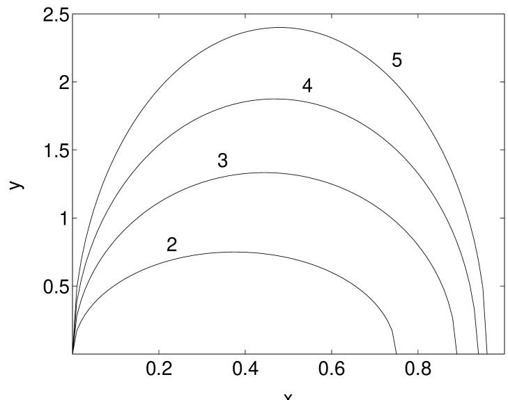
Figure 1: Photon-transverse momentum $y=q_{2\bot}/m_{\pi}$ as a function of $x$ for fixed values of the Compton mass $w=\sqrt{s}/m_{\pi}=2,$ 3, 4, 5. The threshold value, $w=1$, corresponds to the point $y=x=0$.

III Low-mass-Compton region

Hard-pion bremsstrahlung offers a unique possibility of determining pion-threshold polarizabilities. However, this will succeed only if we restrain the c.m. mass in the pion-photon system to masses well below the $\rho$-meson mass, so as to avoid the $s$-channel $\rho$-exchange contribution to the Compton amplitude.

Hence, we first concentrate our efforts on the region $s\ll m_{\rho}^{2}$, where we can confidently approximate the structure functions $A(x,\mathbf{q}_{2\bot}^{2})$ and $B(x,\mathbf{q}_{2\bot}^{2})$ of Eqs.(8) and (9) by their near-threshold values, with

$$\lambda_{1}(x,\mathbf{q}_{2\bot}^{2}) = \frac{m_{\pi}^{3}}{\alpha}\ (\alpha_{\pi}+\beta_{\pi})=0.0006,$$ (19)

$$\lambda_{2}(x,\mathbf{q}_{2\bot}^{2}) = \frac{m_{\pi}^{3}}{\alpha}\ \beta_{\pi}=-0.0131,$$ (20)

and $\alpha_{\pi}$ and $\beta_{\pi}$ the standard pion-electric and pion-magnetic polarizabilities. These values given are obtained in the meson-exchange model when fixing the $\sigma$-meson coupling so that the chiral Lagrangian value Hol of $\lambda_{2}$ is reproduced. Our present knowledge of the pion polarizabilities is reviewed in Ahrens .

The cross-section distribution (3) contains angular dependent terms, through $\mu=\hat{\mathbf{q}}_{1\bot}\cdot\hat{\mathbf{q}}_{2\bot}$. Measured variables are however $\mathbf{q}_{2\bot}$ and $\mathbf{p}_{2\bot}$, but since, $\mathbf{p}_{2\bot}=\mathbf{q}_{1\bot}-\mathbf{q}_{2\bot}$, with ${q}_{1\bot}\ll{q}_{2\bot}$, the angular variations of $\mathbf{q}_{2\bot}$ and $\mathbf{q}_{1\bot}$ are independent. Thus, the integrations over the angles of $\mathbf{q}_{2\bot}$ and $\mathbf{q}_{1\bot}$ in Eq.(3) are unrestricted and we may replace $\mu^{2}$ by its angular average, which is a half, and at the same make the replacement

$$\textrm{d}^{2}q_{1\bot}\textrm{d}^{2}q_{2\bot}=\pi^{2}\textrm{d}q_{1\bot}^{2}\textrm{d}q_{2\bot}^{2}.$$ (21)

After integration over angles the cross-section distribution factorizes into factors that depend either on ${q}_{1\bot}$ and $x$, or on ${q}_{2\bot}$ and $x$. The integration over the inelastic-Coulomb factor (10) is an integration over ${q}_{1\bot}$, but there is an $x$ dependence in $q_{min}$,

$$q_{min}=\frac{m_{\pi}^{2}}{2E_{1}}\cdot\frac{x}{1-x}.$$ (22)

It is tempting to integrate over all possible momentum transfers ${q}_{1\bot}$, but that is not possible since the integral diverges. The reason is that we have neglected pion and nuclear form factors. Also, for large values of ${q}_{1\bot}$ the hadronic-bremsstrahlung contribution dominates the Coulomb contribution. Consequently, we must make a cut so as to avoid the hadronic contribution. The best approach is to make a cut in the same way for all $x$ values. This is achieved by cutting off the integral at $r_{-}q_{min}$ on the low-momentum side and at $r_{+}q_{min}$ on the high-momentum side of the Coulomb peak. From (10) we derive

$$P_{f}\equiv P(r_{-},r_{+})=\int_{r_{-}q_{min}}^{r_{+}q_{min}}\textrm{d}{q}_{1\bot}^{2}\frac{\mbox{\boldmath{${q}$}}_{1\bot}^{2}}{(\mbox{\boldmath{${q}$}}_{1\bot}^{2}+q_{min}^{2})^{2}}.$$ (23)

This integral is obviously independent of $x$. The precise values of $r_{-}$ and $r_{+}$ to be chosen can only be decided after inspection of the experimental distribution.

Next we integrate the cross-section distribution Eq.(3) over transverse-photon momenta in the domain $0\leq q_{2\bot}^{2}\leq q_{2\bot max}^{2}$. Since the polarizability functions $\lambda_{1}$ and $\lambda_{2}$ entering the structure functions $A(x,\mathbf{q}_{2\bot}^{2})$ and $B(x,\mathbf{q}_{2\bot}^{2})$ of Eqs.(8) and (9) are now constants the integration is straightforward, and we get

$$\frac{\textrm{d}\sigma(x,q_{2\bot max})}{\textrm{d}x}=\frac{4Z^{2}\alpha^{3}}{m_{\pi}^{2}}\cdot\frac{1-x}{x}\ P_{f}F(z),$$ (24)

with

$$z(x,q_{2\bot max})=\frac{q_{2\bot max}^{2}}{x^{2}m_{\pi}^{2}}$$ (25)

and the distribution function

$$F(z)=u(z)+\frac{2x^{2}}{1-x}\left(-\frac{1}{4}v(z)\lambda_{1}+\frac{1}{2}w(z)\lambda_{2}\right).$$ (26)

The $x$-dependent prefactor in Eq.(24) is simply the ratio of the final state momenta, $(1-x)/x=E_{2}/\omega_{2}$, and the singularity at $x\approx 0$ is the well-known soft-photon-radiation singularity.

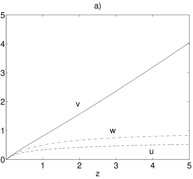
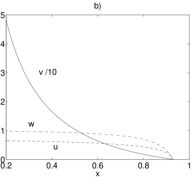
Figure 2: Plots of $u$, $v$, and $w$ as a) functions of $z$; and b) functions of $x$ for $\sqrt{s_{max}}=3.75m_{\pi}$. In b) we have plotted $v/10$ instead of $v$.

The functions $u(z)$, $v(z)$, and $w(z)$, of Eq.(26) are all elementary and given in the Appendix. They are graphed in Fig.2a. For small values of the argument $z$, or transverse momenta such that $q_{2\bot max}^{2}\ll x^{2}m_{\pi}^{2}$, we have

$$u(z)\approx v(z)\approx w(z)\approx z.$$ (27)

For large values of the argument $z$, or transverse momenta such that $q_{2\bot max}^{2}\gg x^{2}m_{\pi}^{2}$, we have instead

$$u(z)\approx\frac{2}{3},\quad v(z)\approx z,\quad w(z)\approx 1.$$ (28)

In particular we note for large values of $z$ the ratio $u(z)/w(z)=2/3$.

An alternative to integrating over transverse-photon momenta is to integrate over Compton masses $\sqrt{s}$ in the domain $m_{\pi}^{2}\leq s\leq s_{max}$. This is simply achieved by making the integration limit $q_{2\bot max}$ depend on $s_{max}$. According to Eq.(17), or (14), the relation between $q_{2\bot max}$ and $s_{max}$ allows us to write

$$z(x,s_{max})=\frac{q_{2\bot max}^{2}}{x^{2}m_{\pi}^{2}}=\frac{s_{max}}{xm_{\pi}^{2}}(x_{max}-x),$$ (29)

with

$$x_{max}=1-\frac{m_{\pi}^{2}}{s_{max}}.$$ (30)

At the same time as being the definition of the variable $z$, Eq.(29) displays the functional relation between $q_{2\bot max}$ and $s_{max}$.

We now specialize to $\sqrt{s_{max}}=3.75m_{\pi}$ which is the cut for the threshold region employed by the COMPASS collaboration. This implies, via Eq.(30), a maximal $x$-value of $x_{max}=0.93$. In Fig.2b the three distribution functions $u$, $v/10$, and $w$ are plotted as functions of $x$ for this value of $s_{max}$. From this figure we draw the following conclusions.

Near the upper end of the $x$-distribution the three functions $u$, $v$, and $w$, may be approximated by their threshold values, Eq.(27). This is a consequence of Eq.(29), which demonstrates that even though the factor $s_{max}/m_{\pi}^{2}=14$ is large, when $x$ is sufficiently close to $x_{max}$ the variable $z$ will be small. This observation leads to a simplification of the cross-section-distribution function $F(z)$ of Eq.(26),

$$F(z)=u(x,s_{max})\left[1+\frac{s_{max}}{m_{\pi}^{2}}(\lambda_{2}-\mbox{${\textstyle\frac{1}{2}}$}\lambda_{1})\right].$$ (31)

Numerically, we expect $\lambda_{2}-\mbox{${\textstyle\frac{1}{2}}$}\lambda_{1}\approx-0.0134$ and small, but enters multiplied by a large factor, $s_{max}/m_{\pi}^{2}$, and therefore makes an important contribution to the cross-section distribution.

In the mid-range $x$-region the value of $z$ is large, due to the large value of $s_{max}/m_{\pi}^{2}$, and we may here approximate the functions $v$ and $w$ by their asymptotic expressions, Eq.(28). This allows us to simplify the expression for the function $F(z)$, yielding the approximate formula

$$F(x,s_{max})=u(x,s_{max})\left[1-\frac{3s_{max}}{4m_{\pi}^{2}}\ x\lambda_{1}+\frac{3x}{2(1-x)}(x\lambda_{2}+\mbox{${\textstyle\frac{1}{2}}$}\lambda_{1})\right].$$ (32)

The function $u(z)$, representing the Born approximation, must be evaluated exactly as we are looking for small deviations from it. The numerical value of the coefficient multiplying the middle $\lambda_{1}$ term in Eq.( 32) is large. Nevertheless, this term has essentially no effect on the cross section since according to Eq.(19) $\lambda_{1}$ is proportional to the sum $\alpha_{\pi}+\beta_{\pi}$ which vanishes, or is very small compared with $\beta_{\pi}$. The important term is the $\lambda_{2}$ term. Over most of the $x$-range its strength is fixed by Eq.(32). But this approximation cannot be used near the upper end-point since it would there overestimate the polarizability contribution by a factor of 3/2, as a comparison with expression (31) would demonstrate.

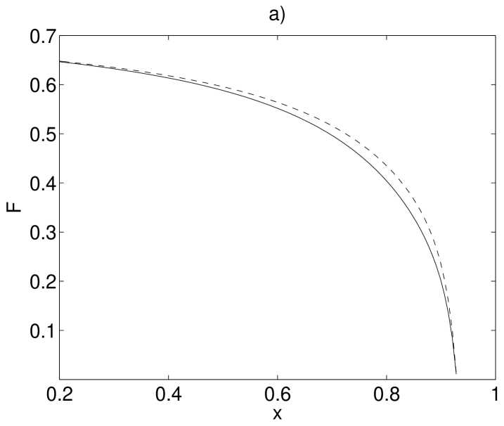
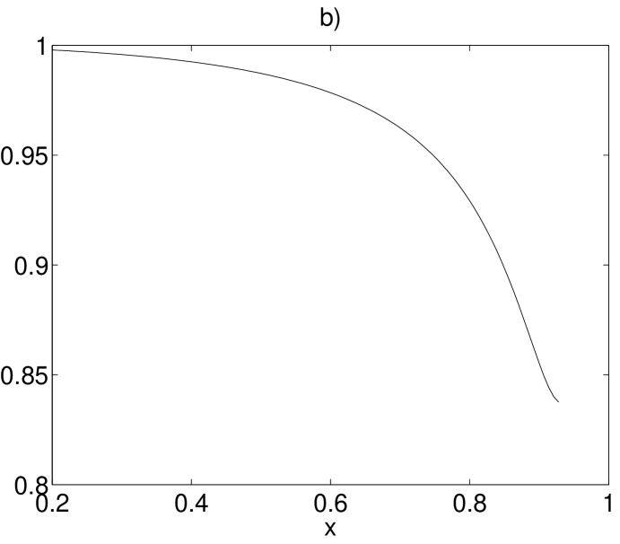
Figure 3: Plots of a) the distribution function $F(z(x,s_{max}))$ of Eq.(26) in the Born approximation (dashed line), and in the full calculation (solid line); and b) the ratio of the two distribution functions.

In Fig.3a the cross-section-distribution function $F(z)$ of Eq.(26) is graphed in the full calculation and in the Born approximation, i.e., when polarizability parameters $\lambda_{1}=\lambda_{2}=0$. In Fig.3b the ratio of the two distributions is plotted. Clearly, the polarizabilities are important only in a region near the end-point of the $x$- distibution, and therefore the experimental efforts are concentrated on this region Ant .

In the COMPASS experiment the apparatus is blind in a small region around the forward direction. The transverse momenta of the final state pions and photons must be larger than $q_{\bot cut}$ to be detected. As a result the distribution function $F(z)$ of Eq.(26) must be replaced by

$$F(z)\rightarrow F(z)-F(z_{0})$$ (33)

where from Eq.(25)

$$z_{0}(x)=\frac{q_{\bot cut}^{2}}{x^{2}m_{\pi}^{2}}\ .$$ (34)

In the COMPASS experiment $q_{\bot cut}=15$ MeV/$c$ and $z_{0}$ is small except when $x$ is near $x=0$. The subtraction procedure of Eq.(33) works unless there are momentum transfers $q_{2\bot}<q_{\bot cut}$ for which $s>s_{max}$. This will not happen as long as $x$ remains in the domain

$$\frac{q_{\bot cut}^{2}}{s_{max}-m_{\pi}^{2}}<x<1-\frac{m_{\pi}^{2}}{s_{max}}-\frac{q_{\bot cut}^{2}}{s_{max}-m_{\pi}^{2}}$$ (35)

which is the case in the COMPASS application. The effect of the cut on the cross section is illustrated in Fig.4.

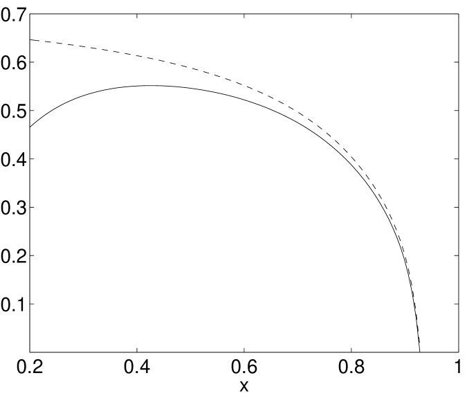
Figure 4: The cross-section-distribution function when small-momentum transfers are cut out according to Eq.(33). The dashed line is the distribution function without the cut, $F(z)$, and the solid line with the cut, $F(z)-F(z_{0})$.

IV Rho-mass-Compton region

At large Compton masses the polarizability functions are complex and depend in a complicated manner on the varables $s$ and $x$. As before, after angular integration, the cross-section distribution factorizes into one factor dependening on $q_{1\bot}$ and $x$, and another one depending on $s$ and $x$.

The integration over the Coulomb-peak factor is unchanged and yields the factor $P_{f}$ of Eq.(23). As the Compton energy $s$ increases and we move closer to the end-point of the $x$ distribution, the minimum-momentum transfer, Eq.(5), increases. The maximal value is obtained at the end-point itself, which is located at $x=1-m_{\pi}^{2}/s$, and where $q_{min}=s/2E_{1}$. At a Compton mass equals the rho mass and an energy $E_{1}=190$ GeV this means $q_{min}=1.5$ MeV$/c$. Away from $x\approx 1$ the value is much smaller.

The angular integration of the right hand side of Eq.(3) is also unchanged. However, it is convenient to replace the variable $q_{2\bot}^{2}$ by $s$, variables which are related by Eq.(11). The cross-section distribution obtained is

$$\frac{\textrm{d}\sigma}{\textrm{d}s\textrm{d}x}=\frac{4Z^{2}\alpha^{3}}{(s-m_{\pi}^{2})^{2}}P_{f}G(x,s).$$ (36)

The distribution function $G(x,s)$ is given by the expresssion

$$G(x,s)=\left|(1-Y(x,s))A(x,s)\right|^{2}+\left|Y(x,s)A(x,s)+B(x,s)\right|^{2},$$ (37)

with $s$ related to $\mathbf{q}_{2\bot}^{2}$ via Eq.(11) and

$$Y(x,s)=\frac{x^{2}m_{\pi}^{2}}{\mathbf{q}_{2\bot}^{2}+x^{2}m_{\pi}^{2}}=\frac{x}{1-x}\cdot\frac{m_{\pi}^{2}}{s-m_{\pi}^{2}},$$ (38)

with the obvious restriction $0\leq Y\leq 1$.

It is instructive to look at the structure functions as functions of $x$ and $s$. From Eqs (8) and (9) we derive the expressions

$$A(x,s) = 1-\frac{1-x}{4}\left(\frac{s-m_{\pi}^{2}}{m_{\pi}^{2}}\right)^{2}\lambda_{1}(x,s),$$ (39)

$$B(x,s) = \frac{x}{2}\left(\frac{s-m_{\pi}^{2}}{m_{\pi}^{2}}\right)\lambda_{2}(x,s).$$ (40)

In the Born approximation $A=1$ and $B=0$, as stated in Eqs.(6) and (7). The Born contribution, which is by far the dominant contribution, is in the cross-section distribution (37) multiplied by the polynomial factor

$$p(Y)=1-2Y+2Y^{2},$$ (41)

with $Y=Y(x,s)$. Since $0\leq Y\leq 1$ it follows that

$$\frac{1}{2}\leq p(Y)\leq 1.$$ (42)

For a fixed value of $s$, the maximal value of the pre-factor, $p(Y)=1$, is obtained at the boundary points $x=0$ and $x=1-m_{\pi}^{2}/s$. The minimum value, $p(Y)=1/2$, is obtained at $x=1-2m_{\pi}^{2}/(s+m_{\pi}^{2})$. Thus, for large values of $s/m_{\pi}^{2}$ there is rapid variation in the kinematical factor $p(Y)$ near the upper end-point of the $x$ region. In the remaining part of phase-space $p(Y)$ is smoothly varying and near to one, since there the variable $Y(x,s)$ itself will be quite small. This is all illustrated in Fig.5.

Figure 5: A contour plot of the kinematic factor $p(Y(x,s))$, or equivalently, the Born approximation to the distribution function $G(x,s)$. Compton mass $s$ in units of $m_{\pi}^{2}$. The dashed line represents the kinematic boundary, where $p(Y)=1$; and the dash-dotted line the minimum, where $p(Y)=1/2$.

The pion structure functions $A$ and $B$ depend on the Mandelstam variables $s$, $t$, and $u$, of the pion-Compton scattering, or equivalently $x$ and $s$. In the region we are considering the Born terms dominate and the polarizability terms mainly come in through their interference with the Born terms. In Fig.6a we plot the quantity $|A-1|^{2}$. From Eq.(39) it is clear that this is a measure of the strength of the $\lambda_{1}$ term. The graph shows that the $\lambda_{1}$ term is small, except for $x$-values near $x=0$, that is grows with $s$ and exhibits a structure related to the $\rho$- and $a_{1}$-meson exchanges.

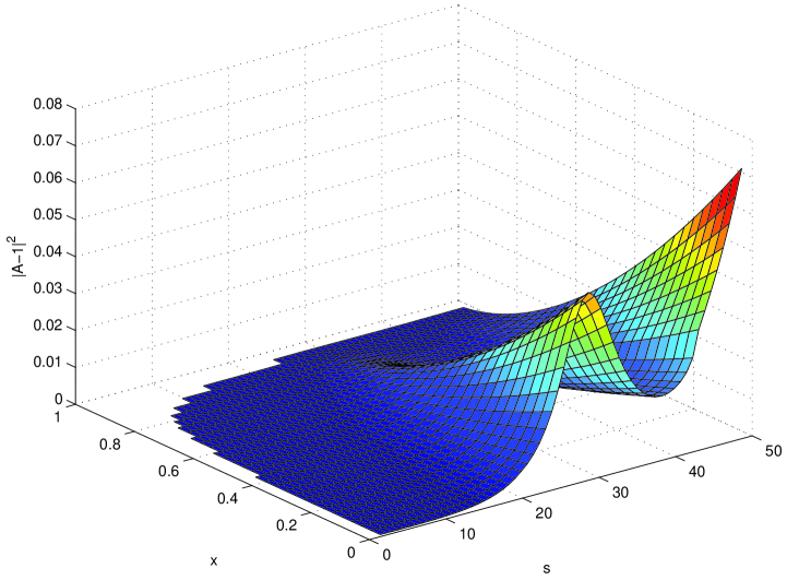
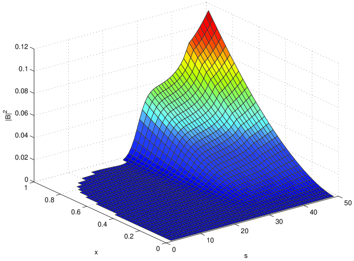
Figure 6: Three-dimensional plots of the functions a) $|A-1|^{2}$ and b) $B^{2}$. Compton mass $s$ in units of $m_{\pi}^{2}$.

In Fig.6b we plot the quantity $|B|^{2}$ which measures the strength of the $\lambda_{2}$ term. The graph demonstrates that $\lambda_{2}$ is important in a region of phase space, essentially disjoint from that of $\lambda_{1}$, namely the region near the upper boundary line of $x$-values. Its strength grows with increasing value of $s$. The structure related to the $\rho$- and $a_{1}$-meson exchanges is visible but less pronounced. It is $\lambda_{2}$ that contains the $\sigma$-meson exchange term. According to Eq.(37) the interference between $B$ and the Born term has an extra factor $Y(x,s)$. This factor results in a sharper structure in the interference term than seen in $B$ alone.

Fig.7 illustrates the behaviour of the dynamic factor $G(x,s)$ of the integrand (37). The plotted quantity is the ratio $G(x,s)/G_{B}(x,s)$, i.e. the ratio of $G(x,s)$ to its Born approximation $G_{B}(x,s)=p(Y)$. We notice that in the overwhelming part of phase space the Born approximation is reasonably accurate. The exceptions are at small $x$-values where the polarizability function $\lambda_{1}$ causes substantial deviations from unity, and at $x$-values near the upper-boundary line where the polarizability function $\lambda_{2}$ contributes to the structure.

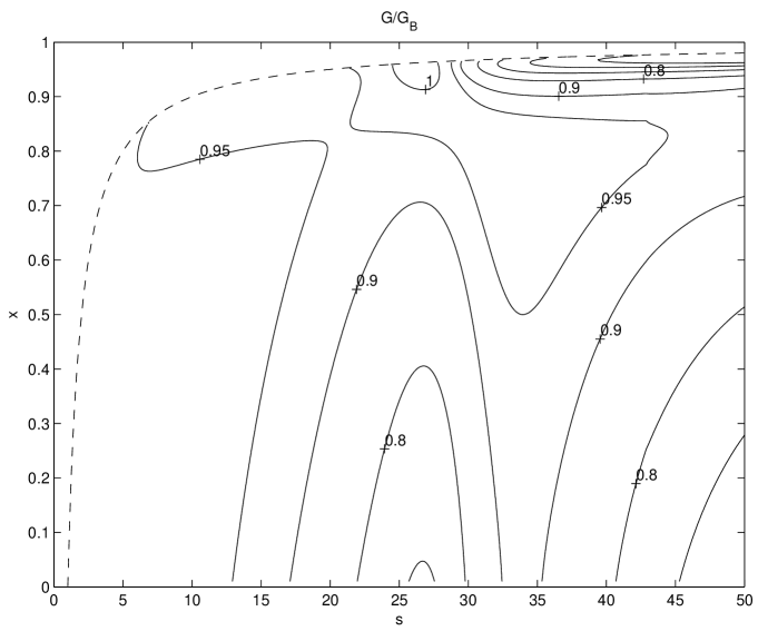
Figure 7: The ratio of the cross-section-distribution function $G(s,x)$ to its Born approximation $G_{B}(x,s)=p(Y)$. The Compton mass $s$ is measured in units of $m_{\pi}^{2}$, and the ratio $x=\omega_{2}/E_{1}$.

Unfortunately, in the latter region precise measurements are complicated by the sharp structure in the distribution function $G(s,x)$.

In Fig.8a the distribution function $G(x,s)$ is graphed as a function of $s$ for fixed $x=0.2$. The dependence on the pion-polarizability functions is strong, with a first dip at the $\rho$-meson mass. As pointed out above this structure is essentially caused by the $\lambda_{1}$ contribution. This is seen already in Eqs.(39) and (40) where the $\lambda_{1}$ contribution is multiplied by the factor $(1-x)$ and the $\lambda_{2}$ contribution by the factor $x$.

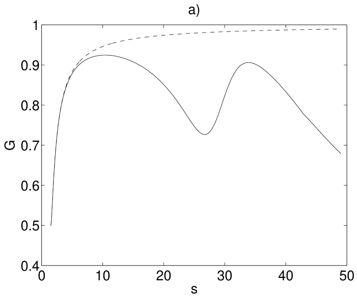
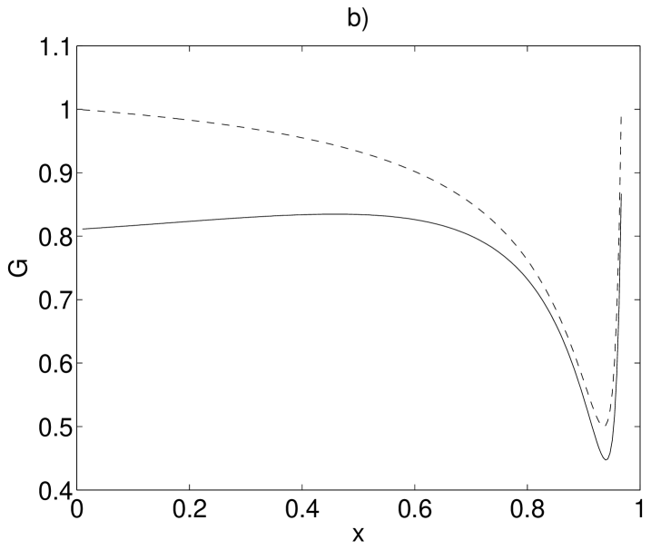
Figure 8: The cross-section-distribution function $G(s,x)$ as a) a function of $s$, in units of $m_{\pi}^{2}$, for $x=0.2$; and as b) a function of $x$ for $s=30$ $m_{\pi}^{2}$.

In Fig.8b the distribution function $G(x,s)$ is instead graphed as a function of $x$ for fixed $s=30$ $m_{\pi}^{2}$. This Compton mass is right on top of the $\rho$-meson mass. Again we observe that the deviation from the Born contribution is larger for small $x$-values than for large $x$-values. Near the upper end-point there is a narrow dip, a structure mainly caused be the $Y$-dependence.

V Summary

Hard bremsstrahlung in high-energy pion-nucleus collisions in the Coulomb region is induced by single photon excitation. Therefore, this reaction can be used to extract information about pion-Compton scattering.

The pion-Compton amplitude is dominated by Born terms that give the exact amplitude for point-like pions. The non-pointlike structure is described by two independent polarizability terms. We describe them in a meson-exchange model with $\sigma$, $\rho$, and $a_{1}$, mesons. The polarizability contributions are small but are important to study. At threshold in the pion-Compton system $\lambda_{1}\propto(\alpha_{\pi}+\beta_{\pi})$ is predicted to vanish and $\lambda_{2}\propto\beta_{\pi}$ predicted to be small. We investigate, through the pion-bremsstrahlung mechanism, the polarizability functions for pion-Compton c.m. energies $s$ below 1 GeV.

In that part of phase space where most of the final-state energy is carried by the photon ($x\approx 1$), the contribution from $\lambda_{1}$ is negligible. The contribution from $\lambda_{2}$ is small but its strength increases with increasing $s$. Some structure caused by the $\rho$-and $a_{1}$-meson exchanges can be seen. At the pion-Compton threshold the contribution from the $\sigma$-exchange term dominates. Experimental efforts to measure the polarizability contributions are at the moment concentrated to this region.

In that part of phase space where most of the final-state energy is carried by the pion ($x\approx 1$), the contribution from $\lambda_{2}$ is negligible. The contribution from $\lambda_{1}$ is clearly seen, and exhibits a strong variation due to the $\rho$-and $a_{1}$-meson exchanges. There is no contribution from $\sigma$ exchange in $\lambda_{1}$.

Our analysis is valid at high energies when the transverse momenta are small compared with the longitudinal momenta. In addition the momentum transfer to the nucleus must be in the Coulomb region, i.e. very small.

VI Acknowledgements

We would like to thank Jan Friedrich for valuable discussions and for information about the COMPASS experiment, and Bengt Karlsson for help with the presentation.

VII Appendix

In Sect.3 we integrate the cross-section distribution Eq.(3) over the photon-transverse momenta $q_{2\bot}$, from the lower limit $q_{2\bot}=0$ up to the upper limit $q_{2\bot}=q_{2\bot max}$. Then, we encounter the following elementary integrals; for the integration of the Born contribution

$$u(z) = z\int_{0}^{q_{2\bot max}^{2}}\frac{\textrm{d}q_{2\bot}^{2}}{q_{2\bot max}^{2}}\left(\frac{x^{2}m_{\pi}^{2}}{\mathbf{q}_{2\bot}^{2}+x^{2}m_{\pi}^{2}}\right)^{2}\left\{1-\frac{2x^{2}m_{\pi}^{2}\mathbf{q}_{2\bot}^{2}}{(x^{2}m_{\pi}^{2}+\mathbf{q}_{2\bot}^{2})^{2}}\right\}$$ (43)

$$= \frac{z}{(1+z)^{2}}+\frac{2z^{3}}{3(1+z)^{3}};$$

for the integration of the $\lambda_{1}$ contribution

$$v(z) = z\int_{0}^{q_{2\bot max}^{2}}\frac{\textrm{d}q_{2\bot}^{2}}{q_{2\bot max}^{2}}\left\{1-\frac{2x^{2}m_{\pi}^{2}\mathbf{q}_{2\bot}^{2}}{(x^{2}m_{\pi}^{2}+\mathbf{q}_{2\bot}^{2})^{2}}\right\}$$ (44)

$$= \frac{2z+z^{2}}{1+z}-\ln(1+z);$$

and for the integration of the $\lambda_{2}$ contribution

$$w(z) = z\int_{0}^{q_{2\bot max}^{2}}\frac{\textrm{d}q_{2\bot}^{2}}{q_{2\bot max}^{2}}\left(\frac{x^{2}m_{\pi}^{2}}{\mathbf{q}_{2\bot}^{2}+x^{2}m_{\pi}^{2}}\right)\left\{1-\frac{\mathbf{q}_{2\bot}^{2}}{x^{2}m_{\pi}^{2}+\mathbf{q}_{2\bot}^{2}}\right\}$$ (45)

$$= \frac{z}{1+z}.$$

The parameter $z$ is defined as

$$z=\frac{q_{2\bot}^{2}}{x^{2}m_{\pi}^{2}}.$$ (46)

References

- (1) A.S. Gal’perin et al., Sov.J.Nucl.Phys. 32 (1980) 545.
- (2) Yu.M. Antipov et al., Phys.Lett. 121B (1983) 445; Yu.M. Antipov et al., Z.Phys. C24 (1984) 39; Yu.M. Antipov et al., Z.Phys. C26 (1984) 495.
- (3) J. Friedrich, Hadron07, Frascati, 8-13 October, 2007.
- (4) G. Fäldt and U. Tengblad, Phys.Rev. C76 (2007) 064607.
- (5) G. Fäldt, Phys.Rev. C76 (2007) 014608.
- (6) J. F. Donoghue and B. R. Holstein, Phys. Rev. D 48, 137 (1993).
- (7) J. Ahrens et al., Eur. Phys. J. A 23, 113 (2005).