UWTHPh-2008-01

Harald Grosse¹, Harold Steinacker², Michael Wohlgenannt³

Fakultät für Physik, Universität Wien
Boltzmanngasse 5, A-1090 Wien, Austria

Erwin Schrödinger International Institute for Mathematical Physics
Boltzmanngasse 9, A-1090 Wien, Austria

Abstract

We verify explicitly that UV/IR mixing for noncommutative gauge theory can be understood in terms of an induced gravity action, as predicted by the identification [1] of gravity within matrix models of NC gauge theory. More precisely, we obtain the Einstein-Hilbert action by integrating out a scalar field in the adjoint. It arises from the well-known UV/IR mixing of NC gauge theory, which is carefully re-analyzed and interpreted in terms of gravity. The matrix model therefore contains gravity as an IR effect, due to UV/IR mixing.

 

 

1 Introduction

The idea that gravity should be related to quantum fluctuations of space-time at the Planck scale is very old. Recently, a specific and concise realization of this idea has been proposed under the name of “emergent (noncommutative) gravity”. The basic observation is that noncommutative (NC) gauge theory, defined through matrix models, contains a specific version of gravity as an intrinsic part, and provides a dynamical theory of noncommutative spaces. Such a connection between gravity and NC gauge theory was first observed in [2], and pushed further in [3] from a somewhat different point of view; see also [4] for subsequent work. A concise form of this idea was then given in [1] using the framework of matrix models. The essential point is a new, geometrical interpretation of the $U(1)$ sector of the standard matrix model action for NC gauge theory. This provides a specific form for the effective metric $G^{ab}$ in terms of a dynamical Poisson structure $\theta^{ab}$, which completely absorbs the “would-be $U(1)$” gauge fields of NC gauge theory. The correct gravitational coupling of the nonabelian gauge fields was also established in [1].

One of the particularly exciting aspects of emergent NC gravity is that it provides a simple prescription for the quantization of gravity, being realized as NC gauge theory resp. Matrix Model. In particular, it was pointed out in [1] that the Einstein-Hilbert action will be induced upon quantization, and that it should amount to the notorious UV/IR mixing in noncommutative gauge theory. This prediction is supported by the fact that both gravity and UV/IR mixing occur only in the $U(1)$ sector of NC gauge theory. It should also explain the strange IR behavior [5] of the “would-be photons”: they are not photons but gravitons defining a non-trivial geometric background. More precisely, the “would-be $U(1)$ gauge fields” are re-interpreted in terms of geometry and absorbed in the effective metric. This metric then couples to all other fields, which explains why the $U(1)$ sector of NC gauge theory cannot be disentangled from the $SU(n)$ sector.

In this paper, we elaborate and verify this explanation of UV/IR mixing in terms of gravity. This provides not only a nontrivial consistency check for emergent NC gravity, it also paves the way towards its quantization. We will perform a one-loop quantization of a scalar field coupled to the matrix model of NC gauge theory resp. gravity in two different ways. In the geometrical point of view, we interpret the action as scalar field coupled to gravity, which leads using standard arguments to an induced Einstein-Hilbert action. Second, we use the more conventional interpretation of the same matrix model in terms of NC gauge theory, where integrating out the scalar field leads to an effective action for the NC gauge fields involving the well-known UV/IR mixing terms [6]. These two computations should agree at least in the IR regime, where the geometrical picture is expected to make sense. We then show in detail that the Einstein-Hilbert action indeed coincides with the effective action for the gauge fields, using the relation between gauge fields and the metric given in [1]. This holds in the IR regime assuming a suitable effective cutoff $\Lambda<\Lambda_{NC}$, where it completely captures the UV/IR mixing. In fact we need to carefully re-analyze the UV/IR mixing terms in this regime, which has not been done in the literature so far.

As a result, we obtain not only a non-trivial check for the basic mechanism of emergent gravity, but also an understanding of UV/IR mixing in NC gauge theory. The latter has been the main obstacle for the physical application of NC gauge theory, because the physical behavior of the trace-$U(1)$ sector forbids an interpretation as a photon. Thus the present point of view opens the way towards the physical application of NC gauge theory resp. the matrix model, and moreover suggests a new approach towards the quantization and unification of gravity and gauge theory. In particular, the effective cutoff is related with the gravitational constant, rather than requiring renormalizability in the traditional sense. This could be realized naturally in a SUSY extension of the model under consideration.

It is interesting to compare our explanation of UV/UR mixing in gauge theory with previous work in the context of string theory, where UV/IR mixing on a brane with $B$-field background was related to the exchange of closed string modes in the bulk [18, 19]. While there are some parallels in the sense that gravity modes are involved, our explanation is certainly simpler and works within the 4-dimensional framework, without additional string modes in some higher-dimensional bulk. Nevertheless, it might be helpful to understand better the relation between these different points of view. Evidence for 4-dimensional gravitons in a quite similar context as ours has been found previously in [28], which is also related to UV/IR mixing.

The paper is organized as follows. We start in section 2 with a recollection of the basic mechanism how geometry and gravity emerges from a matrix model of NC gauge theory. Only $U(1)$ is considered for simplicity. Integrating out a scalar field leads to an induced gravity action as explained in section 3. We then reconsider the same model from the point of view of NC gauge theory in section 4. The geometrical quantities and the induced Einstein-Hilbert action are then expressed in terms of $U(1)$ gauge fields. In section 5, we perform the quantization from the gauge theory point of view, carefully re-analyzing the effective action and UV/IR mixing to $O(A^{2})$. We find indeed complete agreement with the geometrical point of view in a suitable IR regime. Correction terms to the Einstein-Hilbert action are found upon extending this IR regime.

2 Matrix models and effective geometry

Consider the matrix model with action

$$S_{YM}=-Tr[Y^{a},Y^{b}][Y^{a^{\prime}},Y^{b^{\prime}}]g_{aa^{\prime}}g_{bb^{\prime}},$$ (1)

for

$$g_{aa^{\prime}}=\delta_{aa^{\prime}}\quad\mbox{or}\quad g_{aa^{\prime}}=\eta_{aa^{\prime}}$$ (2)

in the Euclidean resp. Minkowski case. While some mathematical aspects of this paper apply mainly to the Euclidean case, we keep the notation general so that the Minkowski case is covered as well at least formally. The ”covariant coordinates” $Y^{a},\,\,a=1,2,3,4$ are hermitian matrices, or equivalently operators acting on a separable Hilbert space ${\cal H}$. We will denote the commutator of 2 matrices as

$$[Y^{a},Y^{b}]=i\theta^{ab}$$ (3)

so that $\theta^{ab}\in L({\cal H})$ is an antihermitian operator-valued matrix, which is not necessarily a multiple of $\mbox{1 \kern-5.89996pt{\rm l}}_{\cal H}$. We focus here on configurations $Y^{a}$ (which need not be solutions of the equation of motion) which can be interpreted via (3) as quantizations of a Poisson manifold $({\cal M},\theta^{ab}(y))$ with general Poisson structure $\theta^{ab}(y)$. This defines the geometrical background under consideration, and conversely essentially any (local) Poisson manifold provides a possible background $Y^{a}$ [7]. More formally, this means that there is an isomorphism of vector spaces

$${\cal C}({\cal M})\to{\cal A}\subset L({\cal H})\,$$ (4)

where ${\cal C}({\cal M})$ denotes some space of functions on ${\cal M}$, and ${\cal A}$ is interpreted as quantized algebra of functions on ${\cal M}$. The map (4) can be used to define a star product on ${\cal C}({\cal M})$. Furthermore, we can then write

$$\left[f,g\right]\sim i\{f(y),g(y)\}$$ (5)

for $f,g\in{\cal A}$, where $\sim$ denotes the leading term in a semi-classical expansion in $\theta^{ab}$, and $\{f,g\}$ the Poisson bracket defined by $\theta^{ab}(y)$. $Y^{a}$ can be interpreted as quantization of a classical coordinate function $y^{a}$ on ${\cal M}$. More importantly, $Y^{a}$ defines a derivation on ${\cal A}$ via

$$[Y^{a},f]\sim i\theta^{ab}(y)\partial_{b}f(y),\qquad f\in{\cal A}.$$ (6)

In this paper, we restrict ourselves to the “irreducible” case, i.e. we assume that the centralizer of ${\cal A}$ in $\cal{H}$ is trivial. Then any reasonable matrix (“function”) in $L({\cal H})$ can be well approximated by a function of $Y^{a}$. From the gauge theory point of view in section 4, it means that we restrict ourselves to the $\mathfrak{u}(1)$ case; this is the case of interest here since the UV/IR mixing happens in the trace-$\mathfrak{u}(1)$ sector. For the general case see [1].

In order to derive the effective metric on ${\cal M}$, let us now consider a scalar field coupled to the matrix model (1). The only possibility to write down kinetic terms for matter fields is through commutators $[Y^{a},\Phi]\sim i\theta^{ab}(y)\frac{\partial}{\partial y^{b}}\Phi$ using (6). Thus consider the action $S=S_{YM}+S[\Phi]$ where

$$S[\Phi] = -(2\pi)^{2}\,Tr\,\frac{1}{2}\,g_{aa^{\prime}}[Y^{a},\Phi][Y^{a^{\prime}},\Phi]$$ (7)

$$\sim \int d^{4}y\,\rho(y)\,\frac{1}{2}\,G^{ab}(y)\,\frac{\partial}{\partial y^{a}}\Phi(y)\frac{\partial}{\partial y^{b}}\Phi(y).$$

Here $\sim$ indicates the leading contribution in a semi-classical expansion in powers of $\theta^{ab}$, and

$$G^{ab}(y)=\theta^{ac}(y)\theta^{bd}(y)\,g_{cd}\,$$ (8)

is the effective metric on ${\cal M}$ in $y$ coordinates, $ds^{2}=G_{ab}(y)\,dy^{a}dy^{b}$. It plays indeed the role of a gravitational metric, because it enters in the kinetic term for any matter coupled to the matrix model (up to certain density factors). This result also holds for nonabelian gauge fields as shown in [1] and for fermions [8]. The density factor

$$\rho(y)=|\det G_{ab}(y)|^{1/4}=(\det\theta^{ab}(y))^{-1/2}\equiv\Lambda_{NC}^{4}(y)$$ (9)

is the symplectic measure on $({\cal M},\theta^{ab}(y))$, which can be interpreted as “local” non-commutative scale $\Lambda_{NC}$. We will assume in this paper that $\theta^{ab}(y)$ is nondegenerate. Notice that the action (7) is invariant under Weyl rescaling of $\theta^{ab}(y)$ resp. $G^{ab}(y)$. We can therefore write the action as

$$S[\Phi]=\int d^{4}y\,\frac{1}{2}\,\tilde{G}^{ab}(y)\,\partial_{y^{a}}\Phi(y)\partial_{y^{b}}\Phi(y)=\int d^{4}y\,\sqrt{|\tilde{G}_{ab}|}\,\,\frac{1}{2}\,\Phi(y)\Delta_{\tilde{G}}\Phi(y)$$ (10)

where $\Delta_{\tilde{G}}$ is the Laplacian for the unimodular metric

$$\tilde{G}^{ab}(y) = (\det G_{ab})^{1/4}\,G^{ab}(y)=\Lambda_{NC}^{4}(y)\,G^{ab}(y)\,,$$

$$\det\tilde{G}^{ab} = 1\,.$$ (11)

We will often use $\tilde{G}^{ab}$; it is important to remember that it is unimodular only in these $y$ coordinates.

Therefore the Poisson manifold ${\cal M}$ naturally acquires a metric structure $({\cal M},\theta^{ab}(y),G^{ab}(y))$, which is determined by the Poisson structure and the constant background metric $g_{ab}$ as above. Note also that $\theta^{ac}(y)$ can be interpreted as a preferred frame or vielbein, which is however gauge-fixed and does not admit the usual local Lorentz resp. orthogonal transformations. This means that we consider a restricted class of metrics and associated coordinates, where the role of the diffeomorphism group is replaced by the symplectomorphisms respecting $\theta^{ab}(y)$. For a related discussion see [3].

A linearized version of (11) was obtained using a similar reasoning in [2], and the full Seiberg-Witten expansion was given in [9] for the case of scalar fields. However the universal role (up to density factors resp. conformal rescaling) of (8) resp. (11) was only recognized in [1]. Note that this metric is not the pull-back of $g^{ab}$ using the change of coordinates (21), and it is indeed curved in general. It is also easy to see that in 4 dimensions, one cannot obtain the most general geometry from metrics of the form (8). However, one does obtain a class of metrics which is sufficient to describe the propagating (“on-shell”) degrees of freedom of gravity, as well as the Newtonian limit for an arbitrary mass distribution. This is discussed in [1] and will not be repeated here. We only point out that the metrics come in a special gauge, which is sufficient of course. The 2 propagating degrees of freedom (helicities) of gravitational waves are recovered from the 2 propagating helicities of $\mathfrak{u}(1)$ gauge fields, taking advantage of the Poisson tensor $\theta^{ab}(y)$ (38).

Equations of motion.

So far we considered arbitrary background configurations $Y^{a}$ as long as they admit a geometric interpretation. The equations of motion derived from the action (1)

$$[Y^{a},[Y^{a^{\prime}},Y^{b}]]\,g_{aa^{\prime}}=0\,$$ (12)

select on-shell geometries among all possible backgrounds, such as the Moyal-Weyl quantum plane (22). In the present geometric form they amount to Ricci-flat spaces $R_{ab}[\tilde{G}]\sim 0$ [2] at least in the linearized case. However since we are interested in the quantization here, we have to consider general off-shell configurations below.

3 Quantization and induced gravity

Now consider the quantization of our matrix model coupled to a scalar field. In principle, the quantization is defined in terms of a (“path”) integral over all matrices $Y^{a}$ and $\Phi$. In 4 dimensions, we can only perform perturbative computations for the “gauge sector” encoded by $Y^{a}$, while the scalars can be integrated out formally in terms of a determinant. Let us focus here on the effective action obtained by integrating out the scalars,

$$e^{-\Gamma_{\Phi}}=\int d\Phi e^{-S[\Phi]}$$ (13)

which for non-interacting scalar fields is given by

$$\Gamma_{\Phi}=\frac{1}{2}{\rm Tr}\log\frac{1}{2}\Delta_{\tilde{G}}\,.$$ (14)

Here $\Delta_{\tilde{G}}$ is the Laplacian of a scalar field on the classical Riemannian manifold $({\cal M},\tilde{G}^{ab}(y))$ with action (10). Later, we will consider an alternative interpretation as Laplacian of a scalar field on ${\mathbb{R}}^{4}_{\bar{\theta}}$ coupled to an adjoint $U(1)$ gauge field. In Feynman diagram language, (14) will then amount to the sum of all one-loop diagrams with arbitrary numbers of external $A$-lines. The subject of this paper is the comparison between these 2 different computations of $\Gamma_{\Phi}$, once from the point of view of gravity (7), and once from the point of view of NC $U(1)$ gauge theory (26). This will provide an interpretation and understanding of the UV/IR mixing for NC gauge theory in terms of an induced gravitational action (Einstein-Hilbert).

Induced gravity.

We first focus on the geometric point of view. We want to compute the one-loop effective action $\Gamma_{\Phi}$ in terms of these classical geometrical data (which will later be expressed in terms of classical $U(1)$ gauge fields $A_{a}(x)$). For this we write

$${\rm Tr}\Big{(}\log\frac{1}{2}\Delta_{\tilde{G}}-\log\frac{1}{2}\Delta_{0}\Big{)} \sim -{\rm Tr}\int_{0}^{\infty}\frac{d\alpha}{\alpha}\,(e^{-\alpha\frac{1}{2}\Delta_{\tilde{G}}}-e^{-\alpha\frac{1}{2}\Delta_{0}})\,\,$$ (15)

$$\equiv \,\,-{\rm Tr}\int_{0}^{\infty}\frac{d\alpha}{\alpha}\,\Big{(}e^{-\alpha\frac{1}{2}\Delta_{\tilde{G}}}-e^{-\alpha\frac{1}{2}\Delta_{0}}\Big{)}\,e^{-\frac{1}{\alpha\tilde{\Lambda}^{2}}}$$

where the small $\alpha$ divergence is regularized using a UV cutoff $\tilde{\Lambda}$, indicating that it is a cutoff for $\Delta_{\tilde{G}}$. Now we can use the heat kernel expansion,

$${\rm Tr}e^{-\frac{1}{2}\alpha\Delta_{\tilde{G}}}\sim\sum_{n\geq 0}\,(\frac{\alpha}{2})^{\frac{n-4}{2}}\int_{{\cal M}}\,d^{4}y\,\sqrt{|\tilde{G}_{ab}|}\,\,a_{n}(y,\Delta_{\tilde{G}})$$ (16)

where we can drop the measure $\sqrt{\det\tilde{G}}=1$. The $a_{n}(y,\Delta_{\tilde{G}})$ are known as Seeley-de Witt (or Duhamel) coefficients, which for the action (10) are given by [11]

$$a_{0}(y) = \frac{1}{16\pi^{2}}\,,$$

$$a_{2}(y) = \frac{1}{16\pi^{2}}\,\Big{(}\frac{1}{6}R[\tilde{G}]\Big{)},$$

$$a_{4}(y) = \frac{1}{16\pi^{2}}\,\frac{1}{360}\,\left(12{{R_{;\mu}}}^{\mu}+5R^{2}-2R_{\mu\nu}R^{\mu\nu}+2R_{\mu\nu\rho\sigma}R^{\mu\nu\rho\sigma}\right),$$ (17)

for the scalar case under consideration here (where ${\cal E}=0$ and $\det\tilde{G}=1$ in [11]). Thus we obtain

$$\Gamma_{\Phi}=\frac{1}{16\pi^{2}}\,\int d^{4}y\,\left(-2\tilde{\Lambda}^{4}-\frac{1}{6}R[\tilde{G}]\,\tilde{\Lambda}^{2}+O(\log\tilde{\Lambda})\right)\,.$$ (18)

Recall that in general relativity, the term $S_{const}\sim\int d^{4}y\;\sqrt{\tilde{G}}\,\tilde{\Lambda}^{4}$ corresponds to a cosmological constant, and its bad scaling behavior usually poses a major problem. Here we have $\det\tilde{G}=1$, which suggests that this term is essentially trivial. While this argument alone is not quite conclusive, we will find additional strong evidence that the cosmological constant problem is either absent or at least much milder in the present framework. This would be great news, and will be discussed later. In particular, (18) suggests that the effective Newton constant is given by the effective cutoff

$$\frac{1}{G}\sim\tilde{\Lambda}^{2}.$$ (19)

The curvature scalar $R[\tilde{G}]$ for the unimodular metric $\tilde{G}^{ab}$ can be expressed in terms of the curvature scalar $R[G]$ for $G^{ab}$ using

$$R[\tilde{G}] = \rho(y)\left(R[G]+3\Delta_{G}\sigma-\frac{3}{2}\,G^{ab}\partial_{a}\sigma\partial_{b}\sigma\right)\,,$$

$$\Delta_{G}\sigma = G^{ab}\partial_{a}\partial_{b}\sigma-\Gamma^{c}\partial_{c}\sigma,$$

$$\Gamma^{a} = G^{bc}\,\Gamma_{bc}^{a}\,,$$

$$e^{-\sigma(y)} = \rho(y)=(\det G_{ab})^{1/4}\,.$$ (20)

4 Geometry from $\mathfrak{u}(1)$ gauge fields

4.1 Moyal-Weyl point of view.

Let us now rewrite the geometric action (7) in terms of the $\mathfrak{u}(1)$ gauge fields on the flat Moyal-Weyl background ${\mathbb{R}}^{4}_{\theta}$ with generators $X^{a}$. This means that we consider “small fluctuation”

$$Y^{a}=X^{a}+{\cal A}^{a}\,$$ (21)

around the Moyal-Weyl generators $X^{a}$, which are solutions of the equations of motion (12) and satisfy

$$[X^{a},X^{b}]=i\bar{\theta}^{ab}\,.$$ (22)

Here $\bar{\theta}^{ab}$ is a constant antisymmetric tensor. More precisely, we assume that the hermitian matrices ${\cal A}^{a}={\cal A}^{a}(X)\sim{\cal A}^{a}(x)$ can be interpreted (at least “locally”) as smooth functions on ${\mathbb{R}}^{4}_{\bar{\theta}}$. Note that the effective geometry (8) for the Moyal-Weyl plane is indeed flat, given by

$$\bar{g}^{ab} = \bar{\theta}^{ac}\,\bar{\theta}^{bd}g_{cd}\,$$

$$\tilde{g}^{ab} = \Lambda_{NC}^{4}\,\bar{g}^{ab}$$

$$\bar{\rho} = |\det\bar{g}_{ab}|^{1/4}=(\det\bar{\theta}^{ab})^{-1/2}\equiv\Lambda_{NC}^{4}\,.$$ (23)

Consider now the change of variables

$${\cal A}^{a}(x)=-\bar{\theta}^{ab}A_{b}(x)\quad(=i\bar{\theta}^{ab}iA_{b})$$ (24)

where $A_{a}$ is hermitian. Using

$$[X^{a}+{\cal A}^{a},f]=i\bar{\theta}^{ab}(\frac{\partial}{\partial x^{b}}f+i[A_{b},f])\equiv i\bar{\theta}^{ab}D_{b}f,$$ (25)

the action (7) can be written as

$$S[\Phi] = {\rm Tr}\,\frac{1}{2}\bar{\theta}^{ab}\,\bar{\theta}^{a^{\prime}c}g_{aa^{\prime}}\,(\frac{\partial}{\partial x^{b}}\Phi+i[A_{b},\Phi])(\frac{\partial}{\partial x^{c}}\Phi+i[A_{c},\Phi])$$ (26)

$$= \int d^{4}x\,\bar{\rho}\,\frac{1}{2}\bar{g}^{ab}\,(\frac{\partial}{\partial x^{a}}\Phi+i[A_{a},\Phi])(\frac{\partial}{\partial x^{b}}\Phi+i[A_{b},\Phi])$$

$$= \int d^{4}x\,\frac{1}{2}\tilde{g}^{ab}\,D_{a}\Phi D_{b}\Phi=\int d^{4}x\,\frac{1}{2}\,\Phi\Delta_{A}\Phi$$

where we define

$$\Delta_{A}=-\tilde{g}^{ab}\,D_{a}D_{b}=-\bar{\rho}\,[Y^{a},[Y_{a},.]]$$ (27)

using (23). Note that these formulas are exact if interpreted as noncommutative gauge theory on ${\mathbb{R}}^{4}_{\bar{\theta}}$, where $D_{a}=\frac{\partial}{\partial x^{a}}+i[A_{a},.]$ is interpreted as covariant derivative with $\mathfrak{u}(1)$ gauge field $A_{a}(x)$.

4.2 Tensors and coordinate transformation $y\to x$

Let us discuss the tensorial nature of the geometric objects and some associated subtleties. The basic object is the dynamical Poisson structure $\theta^{ab}(y)$ given by (3), which is a rank 2 tensor in $y$ coordinates and satisfies the Jacobi identity $\theta^{ad}(y)\partial_{y^{d}}\theta^{bc}(y)+\mbox{cyclic}=0$. Similarly, the effective metric (31) as well as $g_{ab}$ are tensors in $y$ coordinates. The coordinate system defined by the covariant coordinates $Y^{a}$ resp. $y^{a}$ is the natural one for the geometric point of view and hence for gravity.

On the other hand, using the $\mathfrak{u}(1)$ gauge theory point of view and the change of variables (24) we can express the Poisson tensor in terms of the $\mathfrak{u}(1)$ field strength as

$$i\theta^{ab}(Y)=[Y^{a},Y^{b}]=i\bar{\theta}^{ab}-i\bar{\theta}^{ac}\bar{\theta}^{bd}\,\bar{F}_{cd}\,.$$ (28)

Here $\bar{F}_{ab}=\partial_{x^{a}}A_{b}-\partial_{x^{b}}A_{a}+i[A_{a},A_{b}]$ is a rank 2 tensor in $x$ coordinates on ${\mathbb{R}}^{4}_{\theta}$. This relates the Poisson tensor $\theta^{ab}(y)$ in $y$-coordinates with the field strength tensor $\bar{F}_{cd}$ in $x$-coordinates, where

$$y^{a}=x^{a}-\bar{\theta}^{ab}\,A_{b}\,.$$ (29)

In order to avoid confusion we will denote all $x$-tensors with a bar in this section, and write

$$\partial_{a}=\frac{\partial}{\partial y^{a}},\qquad\bar{\partial}_{a}=\frac{\partial}{\partial x^{a}}\,;$$ (30)

we will drop the bar in later sections if no confusion can arise. Similarly, the induced metric $G^{ab}$ in $y$ coordinates can be written in terms of the $\mathfrak{u}(1)$ gauge fields as

$$G^{ab}(y)=\theta^{ac}(y)\theta^{bd}(y)\,g_{cd}=(\bar{\theta}^{ac}-\bar{\theta}^{ae}\bar{\theta}^{ch}\,\bar{F}_{eh})(\bar{\theta}^{bd}-\bar{\theta}^{bf}\bar{\theta}^{dg}\,\bar{F}_{fg})g_{cd}\,.$$ (31)

Notice that while $\bar{F}_{ab}$ and $\bar{\theta}_{ab}$ are tensors in $x$ coordinates, $G^{ab}$ is a tensor in $y$ coordinates. Therefore if we want to compute e.g. Christoffel symbols, we must be careful to implement the change of variables (29), so that

$$\frac{\partial y^{a}}{\partial x^{b}} = \delta^{a}_{b}-\bar{\theta}^{ac}\,\bar{\partial}_{b}A_{c}=\delta^{a}_{b}-V^{a}_{b},$$

$$V_{b}^{a}(x) = \bar{\theta}^{ad}\,\bar{\partial}_{b}A_{d}(x)$$ (32)

and

$$\partial_{a}=\frac{\partial x^{c}}{\partial y^{a}}\frac{\partial}{\partial x^{c}}\approx\bar{\partial}_{a}+V_{a}^{c}\,\bar{\partial}_{c}$$ (33)

to leading order. The Jacobian is given by

$$\left|\frac{\partial y^{a}}{\partial x^{b}}\right| = \left|\delta^{a}_{b}-V^{a}_{b}\,\right|=1-\bar{\theta}^{ac}\,\frac{\partial A_{c}}{\partial x^{a}}+O(\bar{\theta}^{2})$$ (34)

$$= 1-\frac{1}{2}\bar{\theta}^{ac}\,\bar{F}_{ac}+O(\bar{\theta}^{2})\,.$$

This result holds even to $O(A^{2})$ using (40).

Metric and Poisson tensor

Let us now consider the coordinate transformation $x^{a}\to y^{a}$ (29) for some of these tensors. It is easy to see using (28) that the Poisson tensor $\theta^{ab}(y)$ on $y$-space is related to $\bar{\theta}^{ab}$ on $x$-space ${\mathbb{R}}^{4}_{\theta}$ using the diffeomorphism $x^{a}\to y^{a}$ to leading order in $\bar{\theta}$:

$$\theta^{ab}(y)=(\mbox{1 \kern-5.89996pt{\rm l}}+V)^{a}_{a^{\prime}}(\mbox{1 \kern-5.89996pt{\rm l}}+V)^{b}_{b^{\prime}}\bar{\theta}^{a^{\prime}b^{\prime}}\quad+O(\theta^{3}).$$ (35)

This means that $x^{a}$ can be interpreted as (local) Darboux coordinates for $\theta^{ab}(y)$, at least to the leading (semi-classical) order considered here. The relevance of Darboux coordinates for emergent gravity has been emphasized in [3] in the context of the DBI action; see also [13, 14] for related discussion. However, the effective metric $G^{ab}(y)$ (8) is not obtained from either $g^{ab}$ or $\bar{g}^{ab}$ on ${\mathbb{R}}^{4}_{\theta}$ in this manner:

$$G^{ab}(y)=\theta g\theta^{T}=(\mbox{1 \kern-5.89996pt{\rm l}}+V)\bar{\theta}(\mbox{1 \kern-5.89996pt{\rm l}}+V)^{T}g(\mbox{1 \kern-5.89996pt{\rm l}}+V)\bar{\theta}(\mbox{1 \kern-5.89996pt{\rm l}}+V)^{T}\neq(\mbox{1 \kern-5.89996pt{\rm l}}+V)\bar{g}(\mbox{1 \kern-5.89996pt{\rm l}}+V)^{T}$$ (36)

even to leading order. In particular, $\det G^{ab}=(\det(\mbox{1 \kern-5.89996pt{\rm l}}+V))^{4}\det\bar{g}\neq(\det(\mbox{1 \kern-5.89996pt{\rm l}}+V))^{2}\det\bar{g}$. This is essential, since otherwise $G^{ab}$ would be diffeo-equivalent to a constant metric and hence be flat.

4.3 Rewriting the gravity action on ${\mathbb{R}}^{4}_{\theta}$

We will now rewrite the action $\Gamma_{\Phi}$ (18) in terms of gauge fields on ${\mathbb{R}}^{4}_{\theta}$ to $O(A^{2})$. The metric (31) is given by

$$G^{ab} = (\bar{\theta}^{ac}-\bar{\theta}^{ae}\bar{\theta}^{ch}\,\bar{F}_{eh})(\bar{\theta}^{bd}-\bar{\theta}^{bf}\bar{\theta}^{dg}\,\bar{F}_{fg})g_{cd}\,$$ (37)

$$= \bar{g}^{ab}-h^{ab}$$

where

$$h^{ab} = -\bar{g}^{ad}\,\bar{F}_{df}\bar{\theta}^{fb}-\bar{\theta}^{af}\,\bar{F}_{fd}\,\bar{g}^{bd}-\bar{\theta}^{ae}\,\bar{F}_{eh}\bar{g}^{hg}\,\bar{F}_{gf}\bar{\theta}^{fb}$$ (38)

$$= -\bar{g}^{ad}\,\bar{F}_{df}\bar{\theta}^{fb}-\bar{\theta}^{af}\,\bar{F}_{fd}\,\bar{g}^{bd}\,\,+O(A^{2})\,.$$

This gives the linearized fluctuation resp. graviton in terms of the $\mathfrak{u}(1)$ degrees of freedom. The linearized version was essentially found in [2].

An immediate but important observation is that the contributions linear in $A$ to the one-loop effective action (18) vanish identically. This holds because the metric fluctuations $h^{ab}$ are given by derivatives of $A^{a}$, which vanish under the integral $\int d^{4}y$ at $O(A)$ due to Stokes theorem. From the gauge theory point of view, this amounts to the fact that the vacuum $A=0$ is stable under quantization, i.e. the tadpole contributions vanish. This implies that flat space $Y^{a}=X^{a}$ (22) is a solution of emergent gravity even after quantization. Moreover, the same is expected to hold to all loops (using the gauge theory point of view). This observation is very significant, because it is strongly violated in the context of general relativity due to the induced cosmological constant term $\sim\int d^{4}y\Lambda^{4}\sqrt{|g|}$ : in GR, flat space can only be preserved by very precise fine-tuning of the bare cosmological constant. This is the infamous cosmological constant problem. We see here strong evidence that in the context of emergent gravity from matrix models, this problem appears to be resolved or at least much milder. The basic reason is the constraint (8) on the space of metrics.

In order to compute the determinant of the metric, the following form is more useful

$$G^{ab} = \bar{g}^{ar}\left(\delta_{r}^{b}+\bar{F}_{rf}\bar{\theta}^{fb}+\bar{g}_{ra^{\prime}}\bar{\theta}^{a^{\prime}f}\,\bar{F}_{fd}\bar{g}^{db}\,+\bar{g}_{ra^{\prime}}\bar{\theta}^{a^{\prime}e}\,\bar{F}_{eh}\bar{g}^{hg}\bar{F}_{gf}\bar{\theta}^{fb}\right)$$ (39)

$$\equiv \bar{g}^{ar}\left(\delta_{r}^{b}+X_{r}^{b}\right).$$

To compute the determinant, we use

$$\det(\mbox{1 \kern-5.89996pt{\rm l}}+X)=1+trX+\frac{1}{2}\left((trX)^{2}-tr(X^{2})\right)\quad+O(X^{3})\,.$$ (40)

From (37) we have

$$TrX = \,-2\bar{F}_{rf}\bar{\theta}^{rf}-g^{ef}\bar{F}_{eh}\bar{g}^{hg}\bar{F}_{gf}$$ (41)

using $\bar{\theta}^{fb}\bar{g}_{ba}\bar{\theta}^{f^{\prime}a}=g^{ff^{\prime}}$, and one obtains

$$\frac{\det(G^{ab})}{\det(\bar{g}^{ab})} = 1-2\bar{F}_{rf}\bar{\theta}^{rf}+2(\bar{F}_{rf}\bar{\theta}^{rf})^{2}-\bar{F}_{rf}\bar{\theta}^{fb}\bar{F}_{bf^{\prime}}\bar{\theta}^{f^{\prime}r}$$ (42)

to $O(A^{2})$. This can be simplified further in the effective action where we can use partial integration at this order. Using

$$\int d^{4}x\,\bar{F}_{rf}\bar{\theta}^{fb}\bar{F}_{bf^{\prime}}\bar{\theta}^{f^{\prime}r}=\int d^{4}x\,\frac{1}{2}\bar{F}_{rf^{\prime}}\bar{\theta}^{rf^{\prime}}\bar{F}_{bf}\bar{\theta}^{bf}$$ (43)

we can write

$$\det(G^{ab})=\det(\bar{g}^{ab})\Big{(}1-2\bar{F}_{rf}\bar{\theta}^{rf}+\frac{3}{2}(\bar{F}_{rf}\bar{\theta}^{rf})^{2}\Big{)}\,.$$ (44)

This gives

$$e^{\sigma}=(\det G^{ab})^{1/4}=\det(\bar{g}^{ab})^{1/4}\,\Big{(}1-\frac{1}{2}\bar{F}_{rf}\bar{\theta}^{rf}\,+O(\bar{\theta}^{3})\Big{)},$$ (45)

hence

$$\sigma=\frac{1}{4}\log\det(\bar{g}^{ab})\,-\frac{1}{2}\bar{F}_{rf}\bar{\theta}^{rf}-\frac{1}{8}(\bar{F}_{rf}\bar{\theta}^{rf})^{2}$$ (46)

and

$$\bar{g}^{ab}\partial_{a}\sigma\partial_{b}\sigma=\frac{1}{4}\bar{g}^{ab}\bar{\partial}_{a}(\bar{F}_{rf}\bar{\theta}^{rf})\bar{\partial}_{b}(\bar{F}_{r^{\prime}f^{\prime}}\bar{\theta}^{r^{\prime}f^{\prime}})\,.$$ (47)

noting that $\partial_{a}=\partial_{y^{a}}=\bar{\partial}_{a}$ to this order. We also need

$$\Delta_{G}\sigma=-G^{ab}\partial_{a}\partial_{b}\sigma+\Gamma^{c}\partial_{c}\sigma=-\frac{1}{\sqrt{G_{ab}}}\,\partial_{c}\left(\sqrt{G_{ab}}\,G^{cd}\partial_{d}\sigma\right).$$ (48)

To evaluate this, we need

$$\sqrt{\det G_{ab}}=\sqrt{\det\bar{g}_{ab}}\,(1+\bar{\theta}^{ab}\bar{F}_{ab})\quad+O(A^{2})\,.$$ (49)

Therefore

$$\Delta_{G}\sigma = -\frac{1}{\sqrt{G_{ab}}}\,\partial_{c}\left(\sqrt{G_{ab}}\,G^{cd}\partial_{d}\sigma\right)$$ (50)

$$= -(1-\bar{\theta}^{ab}\bar{F}_{ab})(\bar{\partial}_{c}+V_{c}^{l}\bar{\partial}_{l})\left(G^{cd}(1+\bar{\theta}^{ab}\bar{F}_{ab})(\bar{\partial}_{d}+V_{d}^{l}\bar{\partial}_{l})\sigma\right)\quad+O(A^{3})$$

$$= -\bar{\partial}_{c}\left(\bar{g}^{cd}V_{d}^{l}\bar{\partial}_{l}\sigma\right)-V_{c}^{l}\bar{\partial}_{l}\left(\bar{g}^{cd}\bar{\partial}_{d}\sigma\right)-(1-\bar{\theta}^{ab}\bar{F}_{ab})\bar{\partial}_{c}\left(G^{cd}(1+\bar{\theta}^{ab}\bar{F}_{ab})\bar{\partial}_{d}\sigma\right)$$

$$= -\bar{\theta}^{ls}\bar{\partial}_{l}A_{s}\bar{\partial}^{c}\bar{\partial}_{c}\sigma-\bar{\partial}_{c}(G^{cd}\bar{\partial}_{d}\sigma)+\bar{\theta}^{ab}\bar{F}_{ab}\bar{\partial}^{c}\bar{\partial}_{c}\sigma\quad+\partial(O(A^{2}))$$

$$= -\frac{1}{4}\bar{\theta}^{ab}\bar{F}_{ab}\bar{\partial}^{c}\bar{\partial}_{c}F_{de}\theta^{de}+\frac{1}{2}\bar{\partial}^{c}\bar{\partial}_{c}F_{de}\theta^{de}$$

to the order required, omitting total derivatives of order $O(A^{2})$ but not of order $O(A)$. Note that we used (33) in the 2nd line. Therefore

$$3\Delta_{G}\sigma-\frac{3}{2}G^{ab}\partial_{a}\sigma\partial_{b}\sigma = \frac{3}{2}\bar{\partial}^{a}\bar{\partial}_{a}\bar{F}_{rf}\bar{\theta}^{rf}-\frac{3}{8}\bar{F}_{rf}\bar{\theta}^{rf}\bar{\partial}^{a}\bar{\partial}_{a}\bar{F}_{r^{\prime}f^{\prime}}\bar{\theta}^{r^{\prime}f^{\prime}}.$$ (51)

4.3.1 Ricci tensor and scalar curvature

We recall the standard definitions:

$$\Gamma^{e}_{ab} = \frac{1}{2}G^{ce}\left(\partial_{a}G_{bc}+\partial_{b}G_{ca}-\partial_{c}G_{ab}\right),$$ (52)

$$R^{d}_{abc} = \partial_{b}\Gamma^{d}_{ac}-\partial_{c}\Gamma^{d}_{ab}+\Gamma^{s}_{ac}\Gamma^{d}_{sb}-\Gamma^{s}_{ab}\Gamma^{d}_{sc},$$ (53)

$$R_{ac} = R^{d}_{adc},$$ (54)

$$R = G^{ab}R_{ab}\,.$$ (55)

These are tensors in $y$ coordinates. The effective metric is

$$G^{ab}=\bar{g}^{ab}-h^{ab}$$ (56)

with $h^{ab}$ given by (38). The inverse metric is given by

$$G_{ab}=\bar{g}_{ab}+h_{ab}-h_{ac}h^{c}_{a}+\dots\,,$$ (57)

$$\bar{g}_{ab}=(\bar{g}^{cd})^{-1}_{ab}=\bar{\theta}_{ac}^{-1}\bar{\theta}_{bd}^{-1}g^{cd},$$ (58)

with $\bar{\theta}^{ac}\bar{\theta}_{cd}^{-1}=\delta^{a}_{d}$, yielding the identity

$$\bar{\theta}^{ab}\bar{g}_{bc}\bar{\theta}^{dc}=g^{ad}\,.$$ (59)

Indices are shifted with the metric $\bar{g}^{ab}$ and its inverse. Therefore we obtain for the perturbation $h_{ab}$:

$$h_{ab}\equiv\bar{g}_{ac}\bar{g}_{bd}h^{cd}=-\bar{g}_{bu}\bar{\theta}^{uh}\bar{F}_{ha}-\bar{g}_{au}\bar{\theta}^{uh}\bar{F}_{hb}-\bar{g}_{ac}\bar{g}_{bd}\bar{\theta}^{df}\bar{\theta}^{ce}\bar{g}^{hg}\bar{F}_{eh}\bar{F}_{fg}\,.$$ (60)

The terms of second order in $\theta$ in $h^{ab}$ and $h_{ab}$ contribute to the gravity action only to order higher than $\mathcal{O}(A^{2})$ (using partial integration) and can be dropped here.

When computing these quantities we must be careful to take into account the change of variables $x\to y$ (33). For the Christoffel symbols we get

$$\Gamma^{i}_{kl} = \frac{1}{2}\Big{(}\bar{g}^{im}(\bar{\partial}_{l}+V_{l}^{c}\,\bar{\partial}_{c})h_{mk}+\bar{g}^{im}(\bar{\partial}_{k}+V_{k}^{c}\,\bar{\partial}_{c})h_{ml}-\bar{g}^{im}(\bar{\partial}_{m}+V_{m}^{c}\,\bar{\partial}_{c})h_{kl}$$ (61)

$$-h^{im}\bar{\partial}_{l}h_{mk}-h^{im}\bar{\partial}_{k}h_{ml}+h^{im}\bar{\partial}_{m}h_{kl}\quad+\partial(O(A^{2}))\Big{)}$$

$$=: \bar{\Gamma}^{i}_{kl}+\bar{g}^{im}V_{l}^{c}\,\bar{\partial}_{c}h_{mk}+\bar{g}^{im}V_{k}^{c}\,\bar{\partial}_{c}h_{ml}-\bar{g}^{im}V_{m}^{c}\,\bar{\partial}_{c}h_{kl}$$

to $O(A^{2})$, defining the auxiliary object $\bar{\Gamma}^{i}_{kl}$. To second order in $A$ the curvature tensor also picks up additional terms upon rewriting $\partial_{a}$ with $\bar{\partial}_{a}$, and we have

$$R^{d}_{abc} = \partial_{b}\Gamma^{d}_{ac}-\partial_{c}\Gamma^{d}_{ab}+\Gamma^{s}_{ac}\Gamma^{d}_{sb}-\Gamma^{s}_{ab}\Gamma^{d}_{sc}$$ (62)

$$= \bar{\partial}_{b}\Gamma^{d}_{ac}+V_{b}^{e}\bar{\partial}_{e}\Gamma^{d}_{ac}-\bar{\partial}_{c}\Gamma^{d}_{ab}-V_{c}^{e}\bar{\partial}_{e}\Gamma^{d}_{ab}+\Gamma^{s}_{ac}\Gamma^{d}_{sb}-\Gamma^{s}_{ab}\Gamma^{d}_{sc}$$

$$= \bar{\partial}_{b}\bar{\Gamma}^{d}_{ac}+V_{b}^{e}\bar{\partial}_{e}\bar{\Gamma}^{d}_{ac}-\bar{\partial}_{c}\bar{\Gamma}^{d}_{ab}-V_{c}^{e}\bar{\partial}_{e}\bar{\Gamma}^{d}_{ab}+\bar{\Gamma}^{s}_{ac}\bar{\Gamma}^{d}_{sb}-\bar{\Gamma}^{s}_{ab}\bar{\Gamma}^{d}_{sc}\quad+\partial(O(A^{2}))$$

where we omit $O(A^{2})$ terms which are total derivatives, since we are only interested in the action to $O(A^{2})$. Using partial integration we can write

$$V_{b}^{e}\bar{\partial}_{e}\bar{\Gamma}^{d}_{ac}-V_{c}^{e}\bar{\partial}_{e}\bar{\Gamma}^{d}_{ab} = \bar{\theta}^{ef}\,\bar{\partial}_{b}A_{f}\bar{\partial}_{e}\bar{\Gamma}^{d}_{ac}-\bar{\theta}^{ef}\,\bar{\partial}_{c}A_{f}\bar{\partial}_{e}\bar{\Gamma}^{d}_{ab}=\frac{1}{2}\bar{\theta}^{ef}\bar{F}_{ef}\,(\bar{\partial}_{b}\bar{\Gamma}^{d}_{ac}-\bar{\partial}_{c}\bar{\Gamma}^{d}_{ab})$$ (63)

$$= \frac{1}{2}\bar{\theta}^{ed}\bar{F}_{ed}\,R^{(1)d}_{abc}$$

so that

$$R^{d}_{abc}=\bar{\partial}_{b}\bar{\Gamma}^{d}_{ac}-\bar{\partial}_{c}\bar{\Gamma}^{d}_{ab}+\bar{\Gamma}^{s}_{ac}\bar{\Gamma}^{d}_{sb}-\bar{\Gamma}^{s}_{ab}\bar{\Gamma}^{d}_{sc}+\frac{1}{2}\bar{\theta}^{ef}\bar{F}_{ef}\,R^{(1)d}_{abc}$$ (64)

to $O(A^{2})$. We can compute the Riemann tensor as an expansion in the metric perturbation $h$

$$R^{d}_{abc}=R^{(1)d}_{abc}+R^{(2)d}_{abc}+\dots\,.$$

The first order term is

$$R^{(1)d}_{abc}=\frac{1}{2}\bar{g}^{dm}\bar{\partial}_{b}\bar{\partial}_{a}h_{mc}-\frac{1}{2}\bar{g}^{dm}\bar{\partial}_{b}\bar{\partial}_{m}h_{ac}-\frac{1}{2}\bar{g}^{dm}\bar{\partial}_{c}\bar{\partial}_{a}h_{mb}+\frac{1}{2}\bar{g}^{dm}\bar{\partial}_{c}\bar{\partial}_{m}h_{ab}.$$ (65)

We can now compute the second order term of the Riemann tensor:

$$R^{(2)d}_{abc} = \frac{1}{4}\bigg{(}\bar{g}^{sm}\bar{\partial}_{c}h_{ma}+\bar{g}^{sm}\bar{\partial}_{a}h_{mc}-\bar{g}^{sm}\bar{\partial}_{m}h_{ac}\bigg{)}\,\bigg{(}\bar{g}^{dn}\bar{\partial}_{b}h_{ns}+\bar{g}^{dn}\bar{\partial}_{s}h_{nb}-\bar{g}^{dn}\bar{\partial}_{n}h_{sb}\bigg{)}$$ (66)

$$-\frac{1}{4}\bigg{(}\bar{g}^{sm}\bar{\partial}_{b}h_{ma}+\bar{g}^{sm}\bar{\partial}_{a}h_{mb}-\bar{g}^{sm}\bar{\partial}_{m}h_{ab}\bigg{)}\,\bigg{(}\bar{g}^{dn}\bar{\partial}_{c}h_{ns}+\bar{g}^{dn}\bar{\partial}_{s}h_{nc}-\bar{g}^{dn}\bar{\partial}_{n}h_{sc}\bigg{)}\,$$

$$+\frac{1}{2}\bar{\theta}^{fe}\,\bar{F}_{fe}\,R^{(1)d}_{abc}$$

omitting $O(A^{2})$ terms which are total derivatives. A suitable contraction gives the 2nd order Ricci tensor

$$R^{(2)}_{ac} = \frac{1}{4}\bar{g}^{sm}\bar{g}^{dn}\Big{(}\bar{\partial}_{c}h_{ma}\bar{\partial}_{d}h_{ns}+\bar{\partial}_{c}h_{ma}\bar{\partial}_{s}h_{nd}-\bar{\partial}_{c}h_{ma}\bar{\partial}_{n}h_{sd}+\bar{\partial}_{a}h_{mc}\bar{\partial}_{d}h_{ns}$$

$$+\bar{\partial}_{a}h_{mc}\bar{\partial}_{s}h_{nd}-\bar{\partial}_{a}h_{mc}\bar{\partial}_{n}h_{sd}-\bar{\partial}_{m}h_{ac}\bar{\partial}_{d}h_{ns}-\bar{\partial}_{m}h_{ac}\bar{\partial}_{s}h_{nd}$$

$$+\bar{\partial}_{m}h_{ac}\bar{\partial}_{n}h_{sd}-\bar{\partial}_{d}h_{ma}\bar{\partial}_{c}h_{ns}-\bar{\partial}_{d}h_{ma}\bar{\partial}_{s}h_{nc}+\bar{\partial}_{d}h_{ma}\bar{\partial}_{n}h_{sc}$$

$$-\bar{\partial}_{a}h_{md}\bar{\partial}_{c}h_{ns}-\bar{\partial}_{a}h_{md}\bar{\partial}_{s}h_{nc}+\bar{\partial}_{a}h_{md}\bar{\partial}_{n}h_{sc}+\bar{\partial}_{m}h_{ad}\bar{\partial}_{c}h_{ns}$$

$$+\bar{\partial}_{m}h_{ad}\bar{\partial}_{s}h_{nc}-\bar{\partial}_{m}h_{ad}\bar{\partial}_{n}h_{sc}\Big{)}+\frac{1}{2}\bar{\theta}^{fe}\,\bar{F}_{fe}\,R^{(1)}_{ac}.$$

Using partial integration this can be written as

$$R^{(1)}_{ac} = \bar{\partial}^{s}\bar{\partial}_{(a}h_{c)s}-\frac{1}{2}\bar{\partial}_{a}\bar{\partial}_{c}h-\frac{1}{2}\bar{\partial}^{d}\bar{\partial}_{d}h_{ac}\,,$$ (68)

$$R_{ac}^{(2)} = \frac{1}{4}h^{uv}\bar{\partial}_{a}\bar{\partial}_{c}h_{uv}-\frac{1}{2}h_{m(a}\bar{\partial}_{c)}\bar{\partial}^{m}h+\frac{1}{4}h_{ac}\bar{\partial}^{c}\bar{\partial}_{c}h$$

$$+\frac{1}{2}h_{am}\bar{\partial}^{m}\bar{\partial}^{d}h_{dc}-\frac{1}{2}h^{m}_{a}\bar{\partial}^{c}\bar{\partial}_{c}h_{mc}+\frac{1}{2}\bar{\theta}^{fe}\,\bar{F}_{fe}\,R^{(1)}_{ac}$$

where

$$\bar{\partial}_{(a}h_{c)s}=\frac{1}{2}(\bar{\partial}_{a}h_{cs}+\bar{\partial}_{c}h_{as})\,.$$

The Ricci scalar $R=G^{ab}R_{ab}=R^{(1)}+R^{(2)}=\bar{g}^{ab}R_{ab}^{(1)}+\big{(}-h^{ab}R_{ab}^{(1)}+\bar{g}^{ab}R_{ab}^{(2)}\big{)}$ contains the contributions

$$R^{(1)} = \bar{g}^{ab}R^{(1)}_{ab}=\bar{\partial}^{a}\bar{\partial}^{c}h_{ac}-\bar{\partial}^{c}\bar{\partial}_{c}h,$$ (70)

$$\bar{g}^{ab}R^{(2)}_{ab} = -\frac{1}{2}h_{ac}\bar{\partial}^{a}\bar{\partial}^{c}h+\frac{1}{4}h\bar{\partial}^{c}\bar{\partial}_{c}h+\frac{1}{2}h^{c}_{a}\bar{\partial}^{a}\bar{\partial}^{s}h_{sc}-\frac{1}{4}h^{ac}\bar{\partial}^{c}\bar{\partial}_{c}h_{ac}+\frac{1}{2}\bar{\theta}^{fe}\,\bar{F}_{fe}\,R^{(1)}\,,$$

$$h^{ab}R_{ab}^{(1)} = -\frac{1}{2}\bar{g}^{ma}\bar{g}^{cr}\bar{F}_{rm}\bar{\partial}^{2}\bar{F}_{ca}-\frac{3}{4}\bar{F}_{na}\bar{\theta}^{na}\bar{\partial}^{c}\bar{\partial}_{c}\bar{F}_{mf}\bar{\theta}^{mf}$$ (71)

using (113) and partial integration, where

$$\bar{\partial}^{2}=\bar{\partial}_{a}\bar{\partial}_{b}g^{ab}.$$ (72)

One easily computes in a similar way

$$h = \bar{g}^{cd}h_{cd}=2\bar{\theta}^{ab}\bar{F}_{ab}+\mathcal{O}(A^{2})\,,$$

$$\bar{\partial}^{a}\bar{\partial}^{b}h_{ab} = \bar{\partial}^{a}\bar{\partial}_{a}\bar{\theta}^{uh}\bar{F}_{uh}+\mathcal{O}(A^{2})$$ (73)

so that

$$R^{(1)}=-\bar{\partial}^{a}\bar{\partial}_{a}\bar{\theta}^{uh}\bar{F}_{uh}\,.$$ (74)

The contributions to $\bar{g}^{ab}R^{(2)}_{ab}$ are of the following form:

$$-\frac{1}{2}\int d^{4}x\,h_{ac}\bar{\partial}^{a}\bar{\partial}^{c}h = -\int d^{4}x\,\bar{\theta}^{ab}\bar{F}_{ab}\bar{\partial}^{c}\bar{\partial}_{c}\bar{\theta}^{cd}\bar{F}_{cd}\,,$$ (75)

$$\frac{1}{4}\int d^{4}x\,h\bar{\partial}^{c}\bar{\partial}_{c}h = \int d^{4}x\,\bar{\theta}^{ab}\bar{F}_{ab}\bar{\partial}^{c}\bar{\partial}_{c}\bar{\theta}^{cd}\bar{F}_{cd}\,,$$ (76)

$$\int d^{4}x\,\frac{1}{2}h^{c}_{a}\bar{\partial}^{a}\bar{\partial}^{s}h_{sc}-\frac{1}{4}h^{ab}\bar{\partial}^{c}\bar{\partial}_{c}h_{ab} = \int d^{4}x\left(\frac{1}{8}\bar{\theta}^{ab}\bar{F}_{ab}\bar{\partial}^{c}\bar{\partial}_{c}\bar{\theta}^{cd}\bar{F}_{cd}+\frac{1}{4}\bar{g}^{ah}\bar{g}^{mr}\bar{F}_{hm}\bar{\partial}^{2}\bar{F}_{ra}\right)\,.$$

Collecting these terms, we find

$$\int d^{4}xR^{(2)} = \int d^{4}x\left(\frac{3}{8}\bar{\theta}^{ab}\bar{F}_{ab}\bar{\partial}^{c}\bar{\partial}_{c}\bar{\theta}^{cd}\bar{F}_{cd}+\frac{1}{4}\bar{g}^{ma}\bar{g}^{hr}\bar{F}_{hm}\bar{\partial}^{2}\bar{F}_{ra}\right)\,.$$

We can finally write down the one-loop induced action (18)

$$\Gamma_{\Phi} = \frac{1}{16\pi^{2}}\,\int d^{4}y\,\left(-2\tilde{\Lambda}^{4}-\frac{1}{6}\rho(y)\left(R[G]+3\Delta_{G}\sigma-\frac{3}{2}\,G^{ab}\partial_{a}\sigma\partial_{b}\sigma\right)\tilde{\Lambda}^{2}+O(\log\tilde{\Lambda})\right)$$

$$= \frac{1}{16\pi^{2}}\,\int d^{4}y\,\Bigg{(}-2\tilde{\Lambda}^{4}-\frac{1}{6}\rho(y)\Big{(}\frac{1}{2}\bar{\partial}^{a}\bar{\partial}_{a}\bar{\theta}^{uh}\bar{F}_{uh}+\frac{1}{4}\bar{g}^{ma}\bar{g}^{hr}\bar{F}_{hm}\bar{\partial}^{2}\bar{F}_{ra}\Big{)}\tilde{\Lambda}^{2}\,\,+O(\log\tilde{\Lambda})\Bigg{)}\,.$$

In order to compare this with the gauge theory computation on ${\mathbb{R}}^{4}_{\theta}$, we have to rewrite this action on $x$ space. There is a subtlety concerning the cutoffs: $\tilde{\Lambda}$ is the effective cutoff for $\Delta_{\tilde{G}}$, which acts on the Hilbert space of function with inner product $(f,g)=\int d^{4}y\,f(y)^{*}g(y)$. On the gauge theory side, we have an effective cutoff $\Lambda$ for $\Delta_{A}=\bar{\rho}\,[Y^{a},[Y_{a},.]]$ (27) which acts on the Hilbert space of function with inner product $\left<f,g\right>=Trf^{\star}g=\int d^{4}y\,\rho(y)f(y)^{*}g(y)$. To understand the relation between $\Delta_{\tilde{G}}$ and $\Delta_{A}$ we can write the action in 2 equivalent ways (adding a mass term for clarity)

$$S[\Phi] = \int d^{4}y\,\frac{1}{2}\,\Big{(}-\Phi\partial_{y^{a}}\big{(}\tilde{G}^{ab}(y)\partial_{y^{b}}\Phi\big{)}+\rho(y)m^{2}\Phi^{2}\Big{)}=\int d^{4}y\,\frac{1}{2}\,\Big{(}\Phi\Delta_{\tilde{G}}\Phi+\rho(y)m^{2}\Phi^{2}\Big{)}$$ (79)

$$= Tr\frac{1}{2}\,\Big{(}-\Phi[Y^{a},[Y_{a},\Phi]]+m^{2}\Phi^{2}\Big{)}=\int d^{4}y\,\frac{1}{2}\,\frac{\rho(y)}{\bar{\rho}}\Big{(}\Phi\Delta_{A}\Phi+\bar{\rho}m^{2}\Phi^{2}\Big{)}\,.$$

This means that

$$\Delta_{\tilde{G}}=\frac{\rho(y)}{\bar{\rho}}\,\Delta_{A}$$ (80)

in $y$ coordinates (the gauged kinetic term $\Delta_{A}$ is usually written in $x$ coordinates, but expressed in $y$ coordinates here), which reflects the use of the rescaled metric $\tilde{G}$ (11). Since we implement the cutoffs using a Schwinger parameter as in (15) resp. (94), this means that the effective cutoffs are related as

$$\tilde{\Lambda}^{2}=\frac{\rho(y)}{\bar{\rho}}\,\Lambda^{2}\,.$$ (81)

Such a “local cutoff” makes sense provided $\frac{\rho(y)}{\bar{\rho}}\,$ varies only on large scales resp. small momenta $p\ll\Lambda$, which is indeed our working assumption. The same conclusion is found using a Pauli-Villars regularization (or in a softly broken supersymmetric setting), where the mass $m\sim\Lambda$ in (79) plays the role of the cutoff. Noting that

$$d^{4}y\rho(y) = d^{4}x\bar{\rho}\,,$$

$$\frac{\rho(y)}{\bar{\rho}}\, = \Big{(}\frac{\det G_{ab}}{\det\bar{g}_{ab}}\Big{)}^{1/4}=1+\frac{1}{2}\bar{\theta}^{uh}\bar{F}_{uh}+\frac{1}{4}(F_{ab}\bar{\theta}^{ab})^{2}$$ (82)

we finally obtain

$$\Gamma_{\Phi} = \frac{1}{16\pi^{2}}\,\int d^{4}x\,\Bigg{(}-2\Lambda^{4}(1+\frac{1}{4}(F_{ab}\bar{\theta}^{ab})^{2})-\bar{\rho}\,\frac{\Lambda^{2}}{24}\Big{(}\bar{\theta}^{ab}\bar{F}_{ab}\bar{\partial}^{a}\bar{\partial}_{a}\bar{\theta}^{uh}\bar{F}_{uh}+\bar{g}^{ma}\bar{g}^{hr}\bar{F}_{hm}\bar{\partial}^{2}\bar{F}_{ra}\Big{)}$$ (83)

$$\qquad\qquad+O(\log\Lambda)\,\,+O(A^{3})\Bigg{)}$$

dropping terms which vanish under the integral. This has precisely the form obtained from UV/IR mixing (5.5) in the gauge theory approach.

5 Comparison with UV/IR mixing

In this section, we compare the result of the previous section with the one-loop effective action from the gauge theory point of view. The result is of course the same, but the gauge-theory computation sheds new light on the conditions to which extent the semi-classical analysis of the previous section is valid, and allows to compute corrections to (18). In particular, we find indeed - as predicted in [1] - that the well-known but thus far mysterious UV/IR mixing terms in the effective action for NC gauge theory are precisely given by the induced gravity (=Einstein-Hilbert plus $\Lambda^{4}$ term) action (18), in a suitable IR regime. More precisely, this holds provided

$$p\,\Lambda<\Lambda_{NC}^{2}$$ (84)

which amounts to “mild” UV/IR mixing. In particular, we need an explicit, physical momentum cutoff $\Lambda$, which should typically be of order $\Lambda\leq\Lambda_{NC}$ for the above regime to be physically interesting. In that case, (84) follows from

$$p<\Lambda_{NC},$$ (85)

which is very reasonable range of validity for the classical gravity action. Such a cutoff $\Lambda\leq\Lambda_{NC}$ could be provided e.g. by a softly or spontaneously broken supersymmetric completion of the model, which will be discussed later. Dimensional regularization, on the other hand, does not appear to be useful here.

Even though the one-loop effective action for NC gauge theory has been computed in many places [15, 6, 5, 17, 16], the results given in the literature are not sufficiently precise in the IR limit for our purpose. The point is that we need to analyze carefully the IR regime of the well-known effective cutoff $\Lambda_{eff}(p)$ (101) for non-planar graphs as $p\to 0$, keeping $\Lambda$ fixed. In other words, we consider the regime where the non-planar diagrams almost coincide with the planar diagrams, and keep the leading NC corrections. This corresponds precisely to the leading semiclassical terms inherent in e.g. (6). This regime has not been considered in previous attempts to explain UV/IR mixing, e.g. in terms of exchange of closed string modes [18].

To understand the need for an explicit cutoff $\Lambda$, it is instructive to consider a regularization of ${\mathbb{R}}^{4}_{\theta}$ given e.g. by fuzzy tori [20] or fuzzy ${\mathbb{C}}P^{2}$ resp. $S^{2}\times S^{2}$ [21]. One then typically finds in addition to the NC scale $\Lambda_{NC}$ explicit UV- and IR cutoffs,

$$\Lambda_{IR}=\sqrt{\frac{1}{N\theta}}\quad\ll\quad\Lambda_{NC}=\sqrt{\frac{1}{\theta}}\quad\ll\quad\Lambda_{UV}=\sqrt{\frac{N}{\theta}},$$ (86)

where $N$ is related to the dimension ${\cal N}$ of the matrices (typically ${\cal N}\sim N^{2}$ in 4D). Note that $\Lambda_{UV}=\infty$ for ${\mathbb{R}}^{4}_{\theta}$. This type of fuzzy regularization does not suffice here; if we set $\Lambda=\Lambda_{UV}$, then (84) together with the condition (86) for the semiclassical regime would give $p\leq\Lambda_{IR}$, which leaves no room for interesting physics. Then the geometrical action (18) would have to be replaced by a strongly non-commutative one, which would presumably lead to new phase transitions and new phenomena such as striped phases [22, 23]. In this paper, we focus on the semi-classical regime (84).

5.1 One-loop computation

Consider now the action (26) for a scalar coupled to the $\mathfrak{u}(1)$ gauge field, written in Moyal-Weyl space so that $\bar{\theta}^{ab}=const$. We can cast the action in the form

$$S[\Phi] = \int d^{4}x\,\frac{1}{2}\tilde{g}^{ab}(\bar{\partial}_{a}+ig[A_{a},.])\Phi(\bar{\partial}_{b}+ig[A_{b},.])\Phi+\frac{1}{2}m^{2}\Phi^{2}\,\,=\,\,S_{0}[\Phi]+S_{int}[\Phi],$$

$$S_{0}[\Phi] = \int d^{4}x\,\frac{1}{2}\tilde{g}^{ab}\bar{\partial}_{a}\Phi\bar{\partial}_{b}\Phi+\frac{1}{2}m^{2}\Phi^{2}$$ (87)

with the unimodular metric $\tilde{g}^{ab}$ defined in (23). We introduced an explict coupling constant $g$ and a mass $m$ here. The propagators will involve the metric $\tilde{g}^{ab}$, and we will write

$$k\cdot k \equiv k_{i}k_{j}\,\tilde{g}^{ij}\,,$$

$$k^{2} \equiv k_{i}\,k_{j}g^{ij}$$ (88)

from now on. We need the $O(A^{2})$ contribution to the 1-loop effective action obtained by integrating out the scalar $\Phi$:

$$e^{-\Gamma_{\Phi}}=\left<\exp\Big{(}-\int d^{4}x\,(ig\bar{\partial}_{a}\phi[A_{b},\phi]\tilde{g}^{ab}-\frac{g^{2}}{2}[A_{a},\phi][A_{b},\phi]\tilde{g}^{ab})\Big{)}\right>\,.$$ (89)

While this has been considered several times in the literature, the known results are not accurate enough for our purpose, i.e. in the regime $p^{2},\Lambda^{2}<\Lambda_{NC}^{2}$ where the semiclassical geometry is expected to make sense. We therefore compute carefully

$$\Gamma_{\Phi} = \frac{1}{2}{\rm Tr}\log\Delta_{0}-\frac{g^{2}}{2}\left<\int d^{4}x\,i\bar{\partial}_{a}\phi[A_{b},\phi]\tilde{g}^{ab}\int d^{4}y\,i\bar{\partial}_{a}\phi[A_{b},\phi]\tilde{g}^{ab}\right>$$ (90)

$$-\frac{g^{2}}{2}\left<\int d^{4}x\,[A_{a},\phi][A_{b},\phi]\tilde{g}^{ab}\right>$$

$$= \frac{1}{2}{\rm Tr}\log\Delta_{0}+\Gamma_{\Phi}^{(1)}+\Gamma_{\Phi}^{(2)}.$$

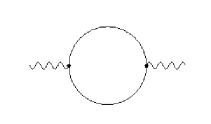
Figure 1:

The contribution from diagram a) in figure 1 is given by

$$\Gamma_{\Phi}^{(1)} = -\frac{g^{2}}{2}\int\frac{d^{4}p}{(2\pi)^{4}}\,A_{a^{\prime}}(p)A_{b^{\prime}}(-p)\tilde{g}^{a^{\prime}a}\tilde{g}^{b^{\prime}b}\int\frac{d^{4}k}{(2\pi)^{4}}\,\frac{4k_{a}k_{b}+2k_{a}p_{b}+2p_{a}k_{b}+p_{a}p_{b}}{(k\cdot k+m^{2})((k+p)\cdot(k+p)+m^{2})}\,$$ (91)

$$\left(1-e^{ik_{i}\theta^{ij}p_{j}}\right)$$

$$= \Gamma_{\Phi}^{(1),P}+\Gamma_{\Phi}^{(1),NP}\,.$$

The contribution from diagram b) in figure 2 is given by

$$\Gamma_{\Phi}^{(2)} = g^{2}\int\frac{d^{4}p}{(2\pi)^{4}}\,A_{a^{\prime}}(p)A_{b^{\prime}}(-p)\tilde{g}^{ab}\int\frac{d^{4}k}{(2\pi)^{4}}\,\frac{1}{(k\cdot k+m^{2})}\,\left(1-e^{ik_{i}\theta^{ij}p_{j}}\right)$$ (92)

$$= \Gamma_{\Phi}^{(2),P}+\Gamma_{\Phi}^{(2),NP}\,.$$

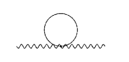
Figure 2:

As a small check, note that the planar and nonplanar parts cancel for $\theta=0$, because $\Phi$ is in the adjoint and decouples for $\theta=0$.

As explained above, in order to compare this with the induced gravity action (18) we must regularize these divergent integrals using a momentum cutoff $\Lambda$. We will do this here “by hand” using a suitable cutoff for the Schwinger parameters. This procedure is applicable for all loops. We will show moreover in Appendix B that precisely this prescription is obtained by carefully implementing the same regularization as in the geometrical action (15). Therefore we should expect to find precise agreement with (18), which is indeed the case.

5.2 Some integrals

We use the Schwinger representation for propagators

$$\frac{1}{k\cdot k+m^{2}} = \int_{0}^{\infty}d\alpha\,e^{-\alpha(k\cdot k+m^{2})},$$

$$\frac{1}{(k\cdot k+m^{2})^{2}} = \int_{0}^{\infty}d\alpha\,\alpha e^{-\alpha(k\cdot k+m^{2})},$$

where $k\cdot k\equiv\tilde{g}^{ij}k_{i}k_{j}$, and put a small mass as an IR regulator. The UV cutoff is conveniently implemented using the following regularization

$$\frac{1}{k\cdot k}\to\int_{0}^{\infty}d\alpha\,e^{-\alpha k\cdot k-\frac{1}{\Lambda^{2}\alpha}}$$ (94)

which removes the UV singularity at $\alpha=0$. For this regularization we need the following integrals:

$$\int_{0}^{\infty}d\alpha\,\frac{1}{\alpha}\,e^{-\alpha m^{2}-\frac{1}{\Lambda^{2}\alpha}} = 2K_{0}\Big{(}2\sqrt{\frac{m^{2}}{\Lambda^{2}}}\Big{)}\,=\,-2\left(\gamma+\log(\sqrt{\frac{m^{2}}{\Lambda^{2}}})\right)\,+O\Big{(}\frac{m^{2}}{\Lambda^{2}}\log(\frac{\Lambda}{m})\Big{)}\,,$$

$$\int_{0}^{\infty}d\alpha\,\frac{1}{\alpha^{2}}\,e^{-\alpha m^{2}-\frac{1}{\Lambda^{2}\alpha}} = 2\sqrt{\Lambda^{2}m^{2}}\,K_{1}(2\sqrt{\frac{m^{2}}{\Lambda^{2}}})$$

$$= \Lambda^{2}-2m^{2}\log(\sqrt{\frac{\Lambda^{2}}{m^{2}}})+m^{2}(2\gamma-1)+O\Big{(}\frac{m^{4}}{\Lambda^{2}}\log(\frac{\Lambda}{m})\Big{)}\,,$$

$$\int_{0}^{\infty}d\alpha\,\frac{1}{\alpha^{3}}\,e^{-\alpha m^{2}-\frac{1}{\Lambda^{2}\alpha}} = 2\Lambda^{2}m^{2}\,K_{2}(2\sqrt{\frac{m^{2}}{\Lambda^{2}}})$$

$$= \Lambda^{4}-m^{2}\Lambda^{2}+m^{4}\log(\sqrt{\frac{\Lambda^{2}}{m^{2}}})-m^{4}(\gamma-\frac{3}{4})+O\Big{(}\frac{m^{6}}{\Lambda^{2}}\log(\frac{\Lambda}{m})\Big{)}$$

where $\gamma$ is the Euler constant. We will drop finite terms which vanish for $m\to 0$, apart from those needed to have dimensionless arguments.

5.3 $\Gamma_{\Phi}^{(1)}$

It is convenient to write (91) using a Feynman parameter

$$\frac{1}{(k\cdot k+m^{2})((k+p)\cdot(k+p)+m^{2})} = \int_{0}^{1}dz\,\frac{1}{(l\cdot l+z(1-z)p\cdot p+m^{2})^{2}}$$ (96)

$$= \int_{0}^{1}dz\,\int_{0}^{\infty}d\alpha\,\alpha e^{-\alpha(l\cdot l+z(1-z)p\cdot p+m^{2})}$$

where

$$l=k+zp\,.$$ (97)

We need

$$\int\frac{d^{4}k}{(2\pi)^{4}}\;\frac{P(k)}{(k\cdot k+m^{2})((k+p)\cdot(k+p)+m^{2})}(1-e^{ik_{i}\theta^{ij}p_{j}})$$

$$= \int\frac{d^{4}k}{(2\pi)^{4}}\;P(k)\int_{0}^{1}dz\,\int_{0}^{\infty}d\alpha\,\alpha e^{-\alpha(l\cdot l+z(1-z)p\cdot p+m^{2})-\frac{1}{\Lambda^{2}\alpha}}(1-e^{ik\theta p})$$

$$= \int_{0}^{1}dz\,\int_{0}^{\infty}d\alpha\,\alpha\,e^{-\alpha(z(1-z)p\cdot p+m^{2})-\frac{1}{\Lambda^{2}\alpha}}\int\frac{d^{4}l}{(2\pi)^{4}}\;P(l-zp)(e^{-\alpha l\cdot l}-e^{-\alpha(l_{i}l_{j}+il_{i}\frac{\tilde{p}_{j}}{\alpha})\tilde{g}^{ij}})$$

$$= \int_{0}^{1}dz\,\int_{0}^{\infty}d\alpha\,\alpha\,e^{-\alpha(z(1-z)p\cdot p+m^{2})-\frac{1}{\Lambda^{2}\alpha}}$$

$$\qquad\int\frac{d^{4}l}{(2\pi)^{4}}\;\left(P(l-zp)e^{-\alpha l\cdot l}-P(l-zp+i\frac{\tilde{p}}{2\alpha})e^{-\alpha l\cdot l-\frac{\tilde{p}\cdot\tilde{p}}{4\alpha}}\right)\,.$$

We completed the square and shifted the integration $l\to l+i\frac{\tilde{p}}{2\alpha}$ in the last expression, where

$$\tilde{p}_{i}=\tilde{g}_{ij}\tilde{p}^{j}=\tilde{g}_{ij}\theta^{jk}p_{k}\,.$$ (98)

For our purpose, $P(k)$ is a polynomial which is at most quadratic. We have

$$\int d^{4}l\;e^{-\alpha l\cdot l} = \pi^{2}\frac{1}{\alpha^{2}},\qquad\int d^{4}l\;l_{i}e^{-\alpha l\cdot l}=0,$$

$$\int d^{4}l\;l_{i}l_{j}e^{-\alpha l\cdot l} = \frac{1}{2}\pi^{2}\tilde{g}_{ij}\,\frac{1}{\alpha^{3}}$$ (99)

since $\det\tilde{g}^{ij}=1$. Therefore

$$\int\frac{d^{4}k}{(2\pi)^{4}}\,\frac{4k_{a}k_{b}+2k_{a}p_{b}+2p_{a}k_{b}+p_{a}p_{b}}{(k\cdot k+m^{2})((k+p)\cdot(k+p)+m^{2})}\,(1-e^{ik\theta p})$$

$$= \frac{1}{16\pi^{2}}\,\int_{0}^{1}dz\,\int_{0}^{\infty}d\alpha\,e^{-\alpha(z(1-z)p\cdot p+m^{2})-\frac{1}{\Lambda^{2}\alpha}}\,\Big{(}p_{a}p_{b}\frac{1}{\alpha}(1-4z+4z^{2})+2g_{ab}\frac{1}{\alpha^{2}}$$

$$-\Big{(}p_{a}p_{b}(1-4z+4z^{2})\frac{1}{\alpha}+i(p_{a}\tilde{p}_{b}+\tilde{p}_{a}p_{b})\frac{1-2z}{\alpha^{2}}-\tilde{p}_{a}\tilde{p}_{b}\frac{1}{\alpha^{3}}+2\tilde{g}_{ab}\frac{1}{\alpha^{2}}\Big{)}e^{-\frac{\tilde{p}\cdot\tilde{p}}{4\alpha}}\Big{)}$$

$$= \frac{1}{16\pi^{2}}\,\int_{0}^{1}dz\,\Big{(}2p_{a}p_{b}(1-4z+4z^{2})\,\Big{(}K_{0}\big{(}{\textstyle 2\sqrt{\frac{z(1-z)p\cdot p+m^{2}}{\Lambda^{2}}}}\big{)}-K_{0}\big{(}{\textstyle 2\sqrt{\frac{z(1-z)p\cdot p+m^{2}}{\Lambda_{eff}^{2}}}}\big{)}\Big{)}$$

$$-\big{(}i(p_{a}\tilde{p}_{b}+\tilde{p}_{a}p_{b})(1-2z)+2\tilde{g}_{ab}\big{)}2\sqrt{(z(1-z)p\cdot p+m^{2})\Lambda_{eff}^{2}}\,K_{1}\big{(}{\textstyle 2\sqrt{\frac{z(1-z)p\cdot p+m^{2}}{\Lambda_{eff}^{2}}}}\big{)}$$

$$+2\tilde{p}_{a}\tilde{p}_{b}(z(1-z)p\cdot p+m^{2})\Lambda_{eff}^{2}\,K_{2}\big{(}{\textstyle 2\sqrt{\frac{z(1-z)p\cdot p+m^{2}}{\Lambda_{eff}^{2}}}}\big{)}$$

$$+2\tilde{g}_{ab}\sqrt{(z(1-z)p\cdot p+m^{2})\Lambda^{2}}\,2K_{1}\big{(}{\textstyle 2\sqrt{\frac{z(1-z)p\cdot p+m^{2}}{\Lambda^{2}}}}\big{)}\Big{)}\Big{)}.$$

This is exact. Note that the term proportional to $(p_{a}\tilde{p}_{b}+\tilde{p}_{a}p_{b})$ vanishes identically under $\int dz$ (as it must, because it is not gauge invariant). Here

$$\Lambda_{eff}^{2} = {1\over 1/\Lambda^{2}+\frac{1}{4}\tilde{p}\cdot\tilde{p}}={1\over 1/\Lambda^{2}+\frac{1}{4}\frac{p^{2}}{\Lambda_{NC}^{4}}}=\Lambda_{eff}^{2}(p)$$ (101)

is the “effective” cutoff for non-planar graphs, noting that

$$\tilde{p}\cdot\tilde{p}=\tilde{p}_{i}\tilde{p}_{j}\tilde{g}^{ij}=\bar{\theta}^{ii^{\prime}}\bar{\theta}^{jj^{\prime}}p_{i^{\prime}}p_{j^{\prime}}\tilde{g}_{ij}=g^{i^{\prime}j^{\prime}}\,p_{i^{\prime}}p_{j^{\prime}}\,(\det\bar{g}^{ab})^{1/4}\equiv\frac{p^{2}}{\Lambda_{NC}^{4}}\,.$$ (102)

Now we consider the IR regime

$$\frac{p^{2}\Lambda^{2}}{\Lambda_{NC}^{4}}<1\,,$$ (103)

see figure 3.

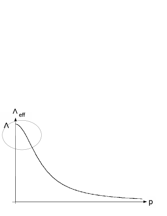
Figure 3: relevant IR regime of $\Lambda_{eff}(p)$

Then both $\Lambda$ and $\Lambda_{eff}$ are large, and we can use the asymptotic expansions (LABEL:K-asymptotics). Thus

$$\int\frac{d^{4}k}{(2\pi)^{4}}\,\frac{4k_{a}k_{b}+2k_{a}p_{b}+2p_{a}k_{b}+p_{a}p_{b}}{(k\cdot k+m^{2})((k+p)\cdot(p+k)+m^{2})}\,(1-e^{ik\theta p})$$

$$\qquad=\frac{1}{16\pi^{2}}\int_{0}^{1}dz\,\Big{(}-p_{a}p_{b}(1-2z)^{2}\,\log\Big{(}\frac{\Lambda_{eff}^{2}}{\Lambda^{2}}\Big{)}$$

$$\qquad\qquad-2\tilde{g}_{ab}\Big{(}\Lambda_{eff}^{2}-\Lambda^{2}+2(z(1-z)p\cdot p+m^{2})\log(\sqrt{\frac{\Lambda^{2}}{\Lambda_{eff}^{2}}})+...\Big{)}$$

$$\qquad\qquad+\tilde{p}_{a}\tilde{p}_{b}\Big{(}\Lambda_{eff}^{4}-(z(1-z)p\cdot p+m^{2})\Lambda_{eff}^{2}$$

$$\qquad\qquad-(z(1-z)p\cdot p+m^{2})^{2}\log\Big{(}\sqrt{{\textstyle\frac{z(1-z)p\cdot p+m^{2}}{\Lambda_{eff}^{2}}}}\Big{)}+...\Big{)}\Big{)}$$

$$\qquad=\frac{1}{16\pi^{2}}\Big{(}-\frac{1}{3}(p_{a}p_{b}-\tilde{g}_{ab}\,p\cdot p)\,\log\Big{(}\frac{\Lambda_{eff}^{2}}{\Lambda^{2}}\Big{)}-2g_{ab}\Big{(}\Lambda_{eff}^{2}-\Lambda^{2}\Big{)}$$

$$\qquad\qquad+\tilde{p}_{a}\tilde{p}_{b}\Big{(}\Lambda_{eff}^{4}-\frac{1}{6}p\cdot p\Lambda_{eff}^{2}+\frac{(p\cdot p)^{2}}{1800}\,(47-30\log({\textstyle\frac{p\cdot p}{\Lambda_{eff}^{2}}}))\Big{)}\Big{)}\,,$$

dropping finite terms vanish for $m\to 0$.

5.4 $\Gamma_{\Phi}^{(2)}$

Here we have

$$\int\frac{d^{4}k}{(2\pi)^{4}}\frac{(e^{ik_{i}\theta^{ij}p_{j}}-1)}{(k\cdot k+m^{2})}\, = \int\frac{d^{4}k}{(2\pi)^{4}}\;\int_{0}^{\infty}d\alpha\,e^{-\alpha(k\cdot k+m^{2})-\frac{1}{\Lambda^{2}\alpha}}(e^{ik\theta p}-1)$$ (104)

$$= \int_{0}^{\infty}d\alpha\,e^{-\alpha m^{2}-\frac{1}{\Lambda^{2}\alpha}}\int\frac{d^{4}k}{(2\pi)^{4}}\;(e^{-\alpha(k-i\frac{\tilde{p}}{2\alpha})\cdot(k-i\frac{\tilde{p}}{2\alpha})-\frac{\tilde{p}\cdot\tilde{p}}{4\alpha}}-e^{-\alpha k\cdot k})$$

$$= \frac{1}{16\pi^{2}}\,2\Big{(}\sqrt{m^{2}\Lambda_{eff}^{2}}K_{1}(2\sqrt{\frac{m^{2}}{\Lambda_{eff}^{2}}})-\sqrt{m^{2}\Lambda^{2}}K_{1}(2\sqrt{\frac{m^{2}}{\Lambda^{2}}})\Big{)}$$

$$\sim \frac{1}{16\pi^{2}}\,\Big{(}\Lambda_{eff}^{2}-\Lambda^{2}+2m^{2}\log(\sqrt{\frac{m^{2}}{\Lambda_{eff}^{2}}})-2m^{2}\log(\sqrt{\frac{m^{2}}{\Lambda^{2}}}\Big{)}$$

$$= \frac{1}{16\pi^{2}}\,\left(\Lambda_{eff}^{2}-\Lambda^{2}\right)$$

up to terms of order $O(m^{2}\frac{p^{2}\Lambda^{2}}{\Lambda_{NC}^{4}})$ which vanish for $m\to 0$.

5.5 Effective action

Combining the above results and using

$$\bar{F}_{ab}(p)\bar{F}_{a^{\prime}b^{\prime}}(-p)\tilde{g}^{aa^{\prime}}\tilde{g}^{bb^{\prime}} = 2\left(p_{a}p_{a^{\prime}}A_{b}(p)A_{b^{\prime}}(-p)-p_{a}p_{b^{\prime}}A_{b}(p)A_{a^{\prime}}(-p)\right)\tilde{g}^{aa^{\prime}}\tilde{g}^{bb^{\prime}}$$

$$(\theta\bar{F}(p))(\theta\bar{F}(-p)) = 4(\tilde{p}^{a}A_{a}(p))(\tilde{p}^{b}A_{b}(-p))$$ (105)

we obtain the induced action

$$\Gamma_{\Phi} = \Gamma_{\Phi}^{(1)}+\Gamma_{\Phi}^{(2)}$$

$$= -\frac{g^{2}}{2}\frac{1}{16\pi^{2}}\,\int\frac{d^{4}p}{(2\pi)^{4}}\,\,\Big{(}-\frac{1}{6}\bar{F}_{ab}(p)\bar{F}_{a^{\prime}b^{\prime}}(-p)\tilde{g}^{a^{\prime}a}\tilde{g}^{b^{\prime}b}\,\log(\frac{\Lambda^{2}}{\Lambda_{eff}^{2}})$$

$$\qquad+\frac{1}{4}(\theta\bar{F}(p))(\theta\bar{F}(-p))\Big{(}\Lambda_{eff}^{4}-\frac{1}{6}p\cdot p\,\Lambda_{eff}^{2}+\frac{(p\cdot p)^{2}}{1800}\,(47-30\log({\textstyle\frac{p\cdot p}{\Lambda_{eff}^{2}}}))\Big{)}\Big{)}$$

up to finite terms vanish for $m\to 0$. This is manifestly gauge invariant.

To make contact with the geometrical action (83), we use the expansions

$$\Lambda_{eff}^{2} = \Lambda^{2}-p^{2}\frac{\Lambda^{4}}{4\Lambda_{NC}^{4}}+...\,,$$

$$\Lambda_{eff}^{4} = \Lambda^{4}-p^{2}\frac{\Lambda^{6}}{2\Lambda_{NC}^{4}}+...\,,$$

$$\log(\frac{\Lambda^{2}}{\Lambda_{eff}^{2}}) = \frac{1}{4}\frac{p^{2}\Lambda^{2}}{\Lambda_{NC}^{4}}+...$$ (107)

which are valid in the IR regime (103). Now assume first

$\Lambda\ll\Lambda_{NC}$.

In this case

$$\Lambda^{6}\frac{p^{2}}{\Lambda_{NC}^{4}}=\frac{\Lambda^{4}}{\Lambda_{NC}^{4}}\Lambda^{2}p^{2}\,\,\ll\,\,\Lambda^{2}p^{2}\,\,\sim\,\,\Lambda^{2}p\cdot p$$ (108)

so that we can replace

$$\Lambda_{eff}^{4}-\frac{1}{6}p\cdot p\Lambda_{eff}^{2}\,\,\sim\,\,\Lambda^{4}-\frac{1}{6}p\cdot p\Lambda^{2}\,.$$ (109)

Then the leading terms are

$$\Gamma_{\Phi} \sim -\frac{g^{2}}{2}\frac{1}{16\pi^{2}}\,\int\frac{d^{4}p}{(2\pi)^{4}}\,\Big{(}\frac{\Lambda^{4}}{4}(\theta\bar{F}(p))(\theta\bar{F}(-p))-\frac{\Lambda^{2}}{24}\bar{F}_{ab}(p)\,\bar{F}_{a^{\prime}b^{\prime}}(-p)\frac{p^{2}}{\Lambda_{NC}^{4}}\tilde{g}^{a^{\prime}a}\tilde{g}^{b^{\prime}b}$$

$$\qquad\qquad\quad-\frac{\Lambda^{2}}{24}(\theta\bar{F}(p))(\theta\bar{F}(-p))p\cdot p\Big{)}$$

$$= -\frac{g^{2}}{2}\frac{1}{16\pi^{2}}\,\int d^{4}x\,\Big{(}\frac{\Lambda^{4}}{4}(\theta\bar{F})(\theta\bar{F})+\bar{\rho}\,\frac{\Lambda^{2}}{24}\Big{(}\bar{F}_{ab}\,\bar{\partial}^{2}\,\bar{F}_{a^{\prime}b^{\prime}}\bar{g}^{a^{\prime}a}\bar{g}^{b^{\prime}b}+(\theta\bar{F})\bar{\partial}^{a}\bar{\partial}_{a}(\theta\bar{F})\Big{)}$$

$$\qquad\qquad+O(\log(\Lambda))\,\,+\rm{finite}\Big{)}\,,$$

using (23) and the notation (72) and (88). This coincides precisely with the effective action obtained from the induced gravity action (83), upon replacing $\Lambda^{2}\to 2\Lambda^{2}$ and absorbing $g$ in $A$. We will show moreover in Appendix B that precisely this prescription is obtained by carefully implementing the same regularization as in the geometrical action (15).

If desired, the $O(\log(\Lambda))$ and finite terms can be obtained from (LABEL:ind-action-gauge). They involve higher derivative expressions, and should reproduce (17); we will not verify this here. Finally, the constant term $-\frac{1}{8\pi^{2}}\int d^{4}x\,\Lambda^{4}$ in (83) represents the phase space volume of states with $\Delta_{0}<\Lambda$, but is physically irrelevant here. It can be obtained if desiresd using the same regularization as above (inserting a test function $f$ for mathematical rigor)

$$-\frac{1}{2}{\rm Tr}\log(\frac{1}{2}\Delta_{0})f = \frac{1}{2}Tr\int_{0}^{\infty}d\alpha\,\frac{1}{\alpha}e^{-\alpha\frac{1}{2}\Delta_{0}}\,e^{-\frac{1}{\Lambda^{2}\alpha}}\,f$$ (110)

$$= -\frac{1}{2}\int\frac{d^{4}k}{(2\pi)^{4}}\,f(k)\int_{0}^{\infty}d\alpha\,\frac{1}{\alpha}e^{-\alpha\frac{1}{2}k\cdot k-\frac{1}{\Lambda^{2}\alpha}}$$

$$= -\frac{1}{2}\Lambda^{4}\,\int\frac{d^{4}k}{(2\pi)^{4}}\,f(k\Lambda)\int_{0}^{\infty}d\alpha\,\frac{1}{\alpha}e^{-\alpha\frac{1}{2}k\cdot k-\frac{1}{\alpha}}$$

$$= -\frac{1}{8\pi^{2}}\Lambda^{4}\,\int d^{4}k\,f(k)\,\delta^{(4)}(k)=-\frac{1}{8\pi^{2}}\Lambda^{4}\,\int d^{4}x\,f(x)$$

using a standard rescaling argument, since $\int d^{4}k\int_{0}^{\infty}d\alpha\,\frac{1}{\alpha}e^{-\alpha\frac{1}{2}k\cdot k-\frac{1}{\alpha}}=4\pi^{2}$. This can also be seen from a theorem by H. Weyl [24] on the asymptotics of eigenvalue distributions.

Let us summarize the main result from the gauge theory point of view. We obtained a simple geometrical explanation of the “strange” IR behavior of NC gauge theory. In particular, the hitherto mysterious $\Lambda^{4}$ divergence reflects the leading term in the density of states of a Laplacian coupled to a background metric, and the $\Lambda^{2}$ terms correspond precisely to the Einstein-Hilbert action. From the gravity point of view, perhaps the most remarkable point is that the $\Lambda^{4}$ term is compatible here with the existence of flat space, unlike in general relativity.

Even though we focused on the IR regime here in order to make contact with the classical geometry, there is nothing which prevents us from considering the effective action also for higher energies. In particular, we obtain a first correction beyond the classical Einstein-Hilbert by assuming

$\Lambda\sim\Lambda_{NC}$.

If $\Lambda\ll\Lambda_{NC}$ does not hold, we cannot neglect $\Lambda^{6}\frac{p^{2}}{\Lambda_{NC}^{4}}$ compared to $\Lambda^{2}p\cdot p$ (108), leading to correction terms in the gravitational action compared with the classical result. For $\Lambda\sim\Lambda_{NC}$, we find

$$\Gamma_{\Phi} \sim -\frac{g^{2}}{2}\frac{1}{16\pi^{2}}\,\int d^{4}x\,\Big{(}\frac{\Lambda^{4}}{4}(\bar{F}\theta)^{2}+\frac{\Lambda^{6}}{4}(\bar{F}\theta)\frac{\bar{\partial}^{2}}{\Lambda_{NC}^{4}}(\bar{F}\theta)$$

$$\qquad\qquad\quad+\bar{\rho}\,\frac{\Lambda^{2}}{24}\Big{(}\bar{F}_{ab}\,\bar{\partial}^{2}\,\bar{F}_{a^{\prime}b^{\prime}}\bar{g}^{a^{\prime}a}\bar{g}^{b^{\prime}b}+(\bar{F}\theta)\bar{\partial}^{a}\bar{\partial}_{a}(\bar{F}\theta)\Big{)}\Big{)}\,.$$

The additional term can be written e.g. as

$$\frac{1}{4}(\bar{F}\theta)\bar{\partial}^{2}(\bar{F}\theta)\sim\sigma\bar{\partial}^{2}\sigma$$ (111)

using (46). Note that its $\Lambda^{6}$ coefficient is somewhat misleading, since it is simply a term in the Taylor expansion of $\Lambda_{eff}^{4}\leq\Lambda^{4}$. Finally, terms quartic in momentum will arise in the action as soon as we violate the IR regime (103), due to higher-order terms in the Taylor expansion of $\Lambda_{eff}$. In that case, one would enter an entirely new regime which is suspected to lead to new types of phenomena and phase transitions (“striped phase”) such as those discussed in [22, 23]. Whether this can be understood in suitably generalized geometrical terms remains to be seen.

6 Conclusion and outlook

In this paper we perform a nontrivial check for the basic result in [1], which gives an interpretation of the $\mathfrak{u}(1)$ sector of NC gauge theory (in the Matrix-Model formulation) in terms of gravity. This provides an explanation of the well-known “strange” IR behavior of the NC gauge theory at the quantum level in terms of an induced Einstein-Hilbert action. We verified this prediction explicitly by comparing the one-loop effective action induced by a scalar field from the geometrical and from the gauge theory point of view. We are able to match and explain the precise form of the UV/IR mixing terms of NC gauge theory to $O(A^{2})$ in the IR limit, including the leading $\Lambda^{4}$ divergence. This confirms the geometric form (18) for the one-loop effective action in the semiclassical limit, as well as the formula (8) for the effective metric. In particular, (18) provides much more information than the 2-particle sector usually considered in NC gauge theory.

The geometric interpretation in terms of an Einstein-Hilbert action applies in the semi-classical IR regime. We therefore consider the IR limit $p\to 0$ of the gauge theory where the well-known “effective cutoff” for the non-planar diagrams $\Lambda_{eff}^{2}=\frac{1}{\frac{1}{\Lambda^{2}}+\frac{1}{4}\tilde{p}\cdot\tilde{p}}$ can be expanded in a Taylor series around $p=0$. The geometrical picture resp. the Einstein-Hilbert action turns out to be valid for momenta $p\Lambda<\Lambda_{NC}^{2}$. This allows a physically reasonable range of momenta $p\leq\Lambda_{NC}$, provided we assume a cutoff $\Lambda<\Lambda_{NC}$. This is a scaling regime which apparently has not been considered in the literature up to now. Moreover, we obtain correction terms to the Einstein-Hilbert action for an extended range of momenta resp. cutoff.

While the gravitational point of view provides an interpretation and understanding of UV/IR mixing, it does not by itself render the theory renormalizable. If we remove the cutoff $\Lambda$ resp. set $\Lambda=\Lambda_{UV}$, the induced gravitational action diverges and cannot be absorbed by adjusting the bare parameters. However, this insight does suggest a way how to make these models well-defined and physically meaningful, by ensuring that there really is a cutoff $\Lambda\leq\Lambda_{NC}$. One natural way to achieve this is to make the model supersymmetric, with spontaneously or softly broken supersymmetry. This should result in a well-defined NC quantum field theory, which contains (emergent) quantized gravity as an intrinsic part. There is indeed an obvious candidate for such a model, namely the IKKT model [25], interpreted as $N=4$ NCSYM in 4 dimensions. This model can be modified e.g. by adding soft SUSY breaking terms. Interestingly enough this provides a direct link with string theory, which may provide further new insights; see also [26, 27] for related work.

Emergent NC gravity therefore provides a new, rather direct link between gravity and gauge theory in 4 dimensions. Some aspects of this relation have been discussed in [3]. We make this relation explicit by expressing the curvature scalar $R[\tilde{G}]$ in terms of $U(1)$ gauge fields. This could be extended to arbitrary $n$-graviton scattering amplitudes, as long as the class of geometries covered by (8) is appropriate. Whether this can be related to other proposed relations between gravity and gauge theory such as [29] remains to be seen. UV/IR mixing for NC gauge theory can now be understood as a relation between the gravitational IR regime of the model and the UV regime which is interpreted in terms of gauge theory. A possible relation with different attempts [30] to identify gravity within the IKKT matrix model is unclear at present.

While some considerations in this paper are mathematically justified only in the Euclidean case, the main ideas apply equally well to the case of Minkowski signature. Therefore the issue of Wick rotation should be re-investigated using the specific assumptions in our context, in particular the restriction to the IR regime (103). Furthermore, we only consider the $U(1)$ case in this paper for simplicity (which means pure gravity); the extension to nonabelian gauge fields was given in [1]. Nevertheless the one-loop quantization of a nonabelian scalar field should be worked out explicitly in the same regime, since it will not only lead to an induced gravity action but also to the (standard) renormalization of the $SU(n)$ gauge fields. We recall that the UV/IR mixing is restricted to the $U(1)$ sector.

Finally, the present computation is a first step towards a complete one-loop computation of the effective action, which then allows to study the physical aspects and viability of emergent gravity. In particular, the cosmological constant problem is expected not to be present or much milder, since flat space remains to be a vacuum solution at one loop. This should provide enough motivation for further work.

Acknowledgments

H.S. would like to thank M. Buric, J. Madore, P. Schupp, and H-S. Yang for discussions, and in particular to L. Freidel and L. Smolin for discussions and hospitality at the Perimeter Institute for theoretical physics. The work of H.S. was supported by the FWF Project P18657, and the work of M.W. was supported in part by the FWF Project P20017 and in part by the Erwin-Schrödinger Institute for mathematical physics.

7 Appendix A: Computation of $h^{ab}R_{ab}$

We compute the leading contribution to $h^{ab}R_{ab}$. To first order in $A$, one finds

$$R^{(1)}_{ab}=-\frac{1}{2}\bar{\theta}^{uh}\bar{\partial}_{a}\bar{\partial}_{b}\bar{F}_{uh}+\frac{1}{2}\bar{\theta}_{a}^{\,\,\,h}\bar{\partial}^{c}\bar{\partial}_{h}\bar{F}_{cb}+\frac{1}{2}\bar{\theta}_{b}^{\,\,\,h}\bar{\partial}^{c}\bar{\partial}_{h}\bar{F}_{ca}\,.$$ (112)

Contraction with the fluctuation of the metric gives

$$\!\!\!\!\!\!\!\!2\int d^{4}xh^{ab}R^{(1)}_{ab}$$ (113)

$$= -\int d^{4}x(\bar{g}^{am}\bar{F}_{mn}\bar{\theta}^{nb}+\bar{g}^{bm}\bar{F}_{mn}\bar{\theta}^{na})(\bar{\theta}_{a}^{\,\,\,h}\bar{\partial}^{c}\bar{\partial}_{h}\bar{F}_{cb}+\bar{\theta}_{b}^{\,\,\,h}\bar{\partial}^{c}\bar{\partial}_{h}\bar{F}_{ca}-\bar{\theta}^{uh}\bar{\partial}_{a}\bar{\partial}_{b}\bar{F}_{uh})$$

$$= -2\int d^{4}x\Big{(}-\bar{g}^{ma}g^{nh}\bar{F}_{mn}\bar{\partial}^{c}\bar{\partial}_{h}\bar{F}_{ca}+\bar{\theta}^{na}\bar{\theta}^{mf}\bar{F}_{mn}\bar{\partial}^{c}\bar{\partial}_{f}\bar{F}_{ca}+\bar{\theta}^{na}\bar{\theta}^{mf}\bar{F}_{cn}\bar{\partial}^{c}\bar{\partial}_{a}\bar{F}_{fm}\Big{)}$$

$$= -\int d^{4}x\Big{(}\bar{g}^{ma}\bar{g}^{cr}\bar{F}_{rm}\bar{\partial}^{2}\bar{F}_{ca}+\frac{3}{2}\bar{F}_{na}\bar{\theta}^{na}\bar{\partial}^{c}\bar{\partial}_{c}\bar{F}_{mf}\bar{\theta}^{mf}\Big{)}$$

where we have used (up to 2nd order in $A$)

• $$\!\!\!\!\!\!\!\!\int d^{4}x\,\bar{g}^{ma}g^{nh}\bar{F}_{mn}\bar{\partial}^{c}\bar{\partial}_{h}\bar{F}_{ca} = -\int d^{4}x\,\bar{g}^{ma}g^{nh}\bar{g}^{cr}\bar{\partial}_{r}\bar{F}_{mn}\bar{\partial}_{h}\bar{F}_{ca}$$

  $$= \int d^{4}x\,\bar{g}^{ma}g^{nh}\bar{g}^{cr}(\bar{\partial}_{m}\bar{F}_{nr}+\bar{\partial}_{n}\bar{F}_{rm})\bar{\partial}_{h}\bar{F}_{ca}$$

  $$= \int d^{4}x\,g^{nh}\bar{g}^{am}\bar{F}_{nm}\bar{\partial}^{c}\bar{\partial}_{h}\bar{F}_{ca}-\bar{g}^{ma}\bar{g}^{cr}\bar{F}_{rm}\bar{\partial}^{2}\bar{F}_{ca}$$

  hence

  $$2\int d^{4}x\,\bar{g}^{ma}g^{nh}\bar{F}_{mn}\bar{\partial}^{c}\bar{\partial}_{h}\bar{F}_{ca}=-\int d^{4}x\,\bar{g}^{ma}\bar{g}^{cr}\bar{F}_{rm}\bar{\partial}^{2}\bar{F}_{ca}$$ (115)

• $$2\int d^{4}x\bar{\theta}^{na}\bar{\theta}^{mf}\bar{F}_{mn}\bar{\partial}^{c}\bar{\partial}_{f}\bar{F}_{ca} = -2\int d^{4}x\bar{\theta}^{na}\bar{\theta}^{mf}\bar{\partial}_{f}\bar{F}_{mn}\bar{\partial}^{c}\bar{F}_{ca}$$

  $$=\int d^{4}x\bar{\theta}^{na}\bar{\theta}^{mf}\bar{\partial}_{n}\bar{F}_{fm}\bar{\partial}^{c}\bar{F}_{ca}=\int d^{4}x\bar{\theta}^{na}\bar{\theta}^{mf}\bar{\partial}^{c}\bar{F}_{fm}\bar{\partial}_{n}\bar{F}_{ca}$$

  $$=\frac{1}{2}\int d^{4}x\bar{\theta}^{na}\bar{\theta}^{mf}\bar{\partial}^{c}\bar{F}_{fm}\bar{\partial}_{c}\bar{F}_{na}=\frac{1}{2}\int d^{4}x\bar{\theta}^{na}\bar{\theta}^{mf}\bar{\partial}^{c}\bar{\partial}_{c}\bar{F}_{mf}\bar{F}_{na}$$

• $$2\int d^{4}x\bar{\theta}^{na}\bar{\theta}^{mf}\bar{F}_{cn}\bar{\partial}^{c}\bar{\partial}_{a}\bar{F}_{fm} = -2\int d^{4}x\bar{\theta}^{na}\bar{\theta}^{mf}\bar{\partial}_{a}\bar{F}_{cn}\bar{\partial}^{c}\bar{F}_{fm}$$

  $$=-\int d^{4}x\bar{\theta}^{na}\bar{\theta}^{mf}\bar{\partial}_{c}\bar{F}_{an}\bar{\partial}^{c}\bar{F}_{fm}=\int d^{4}x\bar{\theta}^{na}\bar{\theta}^{mf}\bar{\partial}^{c}\bar{\partial}_{c}\bar{F}_{na}\bar{F}_{mf}$$

8 Appendix B: Regularization for the gauge theory

Consider the one-loop effective action in terms of the gauge field $A$:

$$\Gamma_{\Phi}=\frac{1}{2}{\rm Tr}\Big{(}\log\frac{1}{2}\Delta_{A}-\log\frac{1}{2}\Delta_{0}\Big{)}\equiv\,\,-\frac{1}{2}{\rm Tr}\int_{0}^{\infty}\frac{d\alpha}{\alpha}\,\Big{(}e^{-\alpha\frac{1}{2}\Delta_{A}}-e^{-\alpha\frac{1}{2}\Delta_{0}}\Big{)}\,e^{-\frac{1}{\alpha\Lambda^{2}}}$$

where the small $\alpha$ divergence is regularized as in (15) using a UV cutoff $\Lambda$. To obtain the expansion in $A$ we use the Duhamel formula (cf. [31])

$$e^{-\alpha H}-e^{-\alpha H^{0}} = -\int_{0}^{\alpha}dt_{1}e^{-t_{1}H^{0}}Ve^{-(\alpha-t_{1})H^{0}}$$ (116)

$$+\int_{0}^{\alpha}dt_{1}\int_{0}^{t_{1}}dt_{2}e^{-t_{2}H^{0}}Ve^{-(t_{1}-t_{2})H^{0}}Ve^{-(\alpha-t_{1})H^{0}}+\dots$$

where $H=H_{0}+V$. Now

$$\int_{0}^{\infty}\frac{d\alpha}{\alpha}\,\int_{0}^{\alpha}dt_{1}\int_{0}^{t_{1}}dt_{2}Tr\Big{(}e^{-t_{2}H^{0}}Ve^{-(t_{1}-t_{2})H^{0}}Ve^{-(\alpha-t_{1})H^{0}}\Big{)}\,e^{-\frac{1}{\alpha\Lambda^{2}}}$$

$$=\int_{0}^{\infty}\frac{d\alpha}{\alpha}\,\int_{0}^{\alpha}dt^{\prime}\,\int_{t^{\prime}}^{\alpha}dt_{1}Tr\Big{(}Ve^{-t^{\prime}H^{0}}Ve^{-(\alpha-t^{\prime})H^{0}}\Big{)}\,e^{-\frac{1}{\alpha\Lambda^{2}}}$$

$$=\int_{0}^{\infty}\frac{d\alpha}{\alpha}\,\int_{0}^{\alpha}dt^{\prime}\,(\alpha-t^{\prime})Tr\Big{(}Ve^{-t^{\prime}H^{0}}Ve^{-(\alpha-t^{\prime})H^{0}}\Big{)}\,e^{-\frac{1}{\alpha\Lambda^{2}}}$$

$$=\int_{0}^{\infty}\frac{d\alpha}{\alpha}\,\int_{0}^{\alpha}dt^{\prime\prime}\,t^{\prime\prime}Tr\Big{(}Ve^{-t^{\prime\prime}H^{0}}Ve^{-(\alpha-t^{\prime\prime})H^{0}}\Big{)}\,e^{-\frac{1}{\alpha\Lambda^{2}}}$$ (117)

where $t^{\prime}=t_{1}-t_{2}$ and $t^{\prime\prime}=\alpha-t^{\prime}$. Combining the two last lines we obtain

$$\int_{0}^{\infty}\frac{d\alpha}{\alpha}\,\int_{0}^{\alpha}dt_{1}\int_{0}^{t_{1}}dt_{2}Tr\Big{(}e^{-t_{2}H^{0}}Ve^{-(t_{1}-t_{2})H^{0}}Ve^{-(\alpha-t_{1})H^{0}}\Big{)}\,e^{-\frac{1}{\alpha\Lambda^{2}}}$$

$$=\frac{1}{2}\,\int_{0}^{\infty}d\alpha\,\int_{0}^{\alpha}dt^{\prime\prime}Tr\Big{(}Ve^{-t^{\prime\prime}H^{0}}Ve^{-(\alpha-t^{\prime\prime})H^{0}}\Big{)}\,e^{-\frac{1}{\alpha\Lambda^{2}}}$$ (118)

so that

$$\Gamma_{\Phi} = \frac{1}{2}\,\int_{0}^{\infty}d\alpha\,{\rm Tr}(Ve^{-\alpha H^{0}})e^{-\frac{1}{\alpha\Lambda^{2}}}-\frac{1}{4}\int_{0}^{\infty}d\alpha\int_{0}^{\alpha}dt^{\prime}\,\,{\rm Tr}\Big{(}Ve^{-t^{\prime}H^{0}}Ve^{-(\alpha-t^{\prime})H^{0}}\Big{)}e^{-\frac{1}{\alpha\Lambda^{2}}}\,.$$

Here ${\rm Tr}$ denotes the trace of operators acting on the scalar field on ${\mathbb{R}}^{4}_{\theta}$, which is conveniently written in momentum basis $\Phi(x)=\int\frac{d^{4}p}{(2\pi)^{4}}\,\Phi(p)\,e^{ip_{a}x^{a}}$. Using

$$(H_{0})_{p,q}=\frac{1}{2}(\Delta_{0})_{p,q}=\frac{1}{2}p^{2}\,\delta_{p,q}$$ (119)

and

$$e^{ikx}e^{ilx}=e^{-\frac{i}{2}k\theta l}\,e^{i(k+l)x}$$ (120)

on ${\mathbb{R}}^{4}_{\theta}$, the interaction term becomes

$$\langle\phi|V|\phi\rangle = \int d^{4}x\,\Big{(}ig\bar{\partial}_{a}\phi[A_{b},\phi]\tilde{g}^{ab}-\frac{g^{2}}{2}[A_{a},\phi][A_{b},\phi]\tilde{g}^{ab}\Big{)}$$ (121)

$$= \int\frac{d^{4}p\,d^{4}q}{(2\pi)^{4}(2\pi)^{4}}\,\Big{(}\phi(p)^{*}\Big{(}\frac{1}{2}g\,(p_{a}+q_{a})A_{b}(p-q)\tilde{g}^{ab}2i\sin(-\frac{1}{2}p\theta q)\Big{)}\phi(q)$$

$$\!\!\!+\int\frac{d^{4}l}{(2\pi)^{4}}\,\phi(p)^{*}\Big{(}\frac{g^{2}}{2}\,A_{a}(l)A_{b}(p-l-q)\tilde{g}^{ab}2\sin(\frac{1}{2}l\theta p)2\sin(-\frac{1}{2}(p-l)\theta q)\Big{)}\phi(q)\Big{)}$$

$$\equiv \int\frac{d^{4}p\,d^{4}q}{(2\pi)^{4}(2\pi)^{4}}\,\Phi(p)^{*}V_{p,q}\Phi(q)\,.$$

Keeping only quadratic expressions in $A$, we obtain

$${\rm Tr}(Ve^{-\alpha H^{0}})=\frac{g^{2}}{2}\,\int\frac{d^{4}l}{(2\pi)^{4}}A_{a}(l)A_{b}(-l)\tilde{g}^{ab}\int\frac{d^{4}p}{(2\pi)^{4}}\,(4\sin^{2}(\frac{1}{2}l\theta p))e^{-\frac{1}{2}p^{2}\,\alpha}$$ (122)

and

$${\rm Tr}\Big{(}Ve^{-t^{\prime}H^{0}}Ve^{-(\alpha-t^{\prime})H^{0}}\Big{)} = \int\frac{d^{4}p\,d^{4}q}{(2\pi)^{4}(2\pi)^{4}}\Big{(}g\,(p_{a}+q_{a})A_{b}(p-q)\tilde{g}^{ab}i\sin(-\frac{1}{2}p\theta q)\Big{)}\,e^{-\frac{1}{2}q^{2}\,t^{\prime}}$$ (123)

$$\Big{(}g\,(p_{a}+q_{a})A_{b}(q-p)\tilde{g}^{ab}i\sin(-\frac{1}{2}q\theta p)\Big{)}\,e^{-\frac{1}{2}p^{2}\,(\alpha-t^{\prime})}$$

$$= g^{2}\int\frac{d^{4}p}{(2\pi)^{4}}A_{b}(p)\tilde{g}^{ab}A_{b^{\prime}}(-p)\tilde{g}^{a^{\prime}b^{\prime}}\int\frac{d^{4}q}{(2\pi)^{4}}(p_{a}+2q_{a})(p_{a^{\prime}}+2q_{a^{\prime}})$$

$$\qquad\sin^{2}(-\frac{1}{2}p\theta q)\,e^{-\frac{1}{2}q^{2}\,t^{\prime}-\frac{1}{2}(p+q)^{2}\,(\alpha-t^{\prime})}\,.$$

Altogether we obtain

$$\Gamma_{\Phi} = g^{2}\int\frac{d^{4}p}{(2\pi)^{4}}A_{a}(p)A_{b}(-p)\tilde{g}^{ab}\int\frac{d^{4}k}{(2\pi)^{4}}\,\sin^{2}(\frac{1}{2}p\theta k)\int_{0}^{\infty}d\alpha\,e^{-\frac{1}{2}k^{2}\,\alpha-\frac{1}{\alpha\Lambda^{2}}}$$ (124)

$$-\frac{g^{2}}{4}\int\frac{d^{4}p}{(2\pi)^{4}}A_{b}(p)\tilde{g}^{ab}A_{b^{\prime}}(-p)\tilde{g}^{a^{\prime}b^{\prime}}\int\frac{d^{4}k}{(2\pi)^{4}}\,(p_{a}+2k_{a})(p_{a^{\prime}}+2k_{a^{\prime}})\sin^{2}(\frac{1}{2}p\theta k)$$

$$\qquad\int_{0}^{\infty}d\alpha\int_{0}^{\alpha}dt^{\prime}\,\,e^{-\frac{1}{2}k^{2}\,t^{\prime}-\frac{1}{2}(p+k)^{2}\,(\alpha-t^{\prime})}e^{-\frac{1}{\alpha\Lambda^{2}}}\,.$$

The first term contains the expected Schwinger parameter, and the second term involves

$$\int_{0}^{\infty}d\alpha\int_{0}^{\alpha}dt^{\prime}\,\,e^{-\frac{1}{2}k^{2}\,t^{\prime}-\frac{1}{2}(p+k)^{2}\,(\alpha-t^{\prime})-\frac{1}{\alpha\Lambda^{2}}}=\int_{0}^{\infty}d\alpha\int_{0}^{\alpha}d\beta\,\,e^{-\frac{1}{2}\alpha(k+\frac{\beta}{\alpha}\,p)^{2}+\frac{1}{2}(\frac{\beta^{2}}{\alpha}-\beta)p\cdot p\,-\frac{1}{\alpha\Lambda^{2}}}$$

where $\beta=\alpha-t^{\prime}$. Define

$$l\equiv k+z\,p,\qquad z=\frac{\beta}{\alpha}\,$$ (125)

so that

$$\int_{0}^{\infty}d\alpha\int_{0}^{\alpha}dt^{\prime}\,\,e^{-\frac{1}{2}k^{2}\,t^{\prime}-\frac{1}{2}(p+k)^{2}\,(\alpha-t^{\prime})}e^{-\frac{1}{\alpha\Lambda^{2}}}=4\int_{0}^{\infty}d\alpha^{\prime}\,\alpha^{\prime}\int_{0}^{1}dz\,\,e^{-\alpha^{\prime}(l^{2}+z(1-z)\,p\cdot p)-\frac{1}{2\alpha^{\prime}\Lambda^{2}}}$$

where

$$\alpha^{\prime}=\alpha/2.$$ (126)

Now

$$\sin^{2}(\frac{1}{2}k\theta p)=\frac{1}{2}(1-\cos(k\theta p))\sim\frac{1}{2}(1-e^{ik\theta p})$$ (127)

provides the distinction between planar and non-planar diagrams; the latter replacement is justified under the integrals in the present context. Thus we end up exactly with the regularization in section 5,

$$\Gamma_{\Phi} = g^{2}\int\frac{d^{4}k}{(2\pi)^{4}}A_{a}(p)A_{b}(-p)\tilde{g}^{ab}\int\frac{d^{4}k}{(2\pi)^{4}}\,(1-e^{ik\theta p})\int_{0}^{\infty}d\alpha^{\prime}\,e^{-k^{2}\,\alpha^{\prime}-\frac{1}{2\alpha^{\prime}\Lambda^{2}}}$$ (128)

$$-\frac{g^{2}}{2}\int\frac{d^{4}p}{(2\pi)^{4}}A_{b}(p)\tilde{g}^{ab}A_{b^{\prime}}(-p)\tilde{g}^{a^{\prime}b^{\prime}}\int\frac{d^{4}k}{(2\pi)^{4}}\,(p_{a}+2k_{a})(p_{a^{\prime}}+2k_{a^{\prime}})(1-e^{ik\theta p})$$

$$\qquad\int_{0}^{\infty}d\alpha^{\prime}\alpha^{\prime}\int_{0}^{1}dz\,\,e^{-\alpha^{\prime}(l^{2}+z(1-z)\,p\cdot p)-\frac{1}{2\alpha^{\prime}\Lambda^{2}}}\,,$$

with $\Lambda^{2}$ replaced by $2\Lambda^{2}$.

References

• [1] H. Steinacker, “Emergent Gravity from Noncommutative Gauge Theory,” JHEP 12, (2007) 049; [arXiv:0708.2426 [hep-th]].
• [2] V. O. Rivelles, “Noncommutative field theories and gravity,” Phys. Lett.  B 558 (2003) 191 [arXiv:hep-th/0212262].
• [3] H. S. Yang, “Instantons and emergent geometry,” arXiv:hep-th/0608013; H. S. Yang, “Emergent gravity from noncommutative spacetime,” arXiv:hep-th/0611174; H. S. Yang, “On The Correspondence Between Noncommuative Field Theory And Gravity,” Mod. Phys. Lett.  A 22 (2007) 1119 [arXiv:hep-th/0612231].
• [4] B. Muthukumar, “U(1) gauge invariant noncommutative Schroedinger theory and gravity,” Phys. Rev.  D 71 (2005) 105007 [arXiv:hep-th/0412069].
• [5] A. Matusis, L. Susskind and N. Toumbas, “The IR/UV connection in the non-commutative gauge theories,” JHEP 0012 (2000) 002 [arXiv:hep-th/0002075].
• [6] S. Minwalla, M. Van Raamsdonk and N. Seiberg, “Noncommutative perturbative dynamics,” JHEP 0002 (2000) 020 [arXiv:hep-th/9912072].
• [7] M. Kontsevich, “Deformation quantization of Poisson manifolds, I,” Lett. Math. Phys.  66 (2003) 157 [arXiv:q-alg/9709040].
• [8] in preparation
• [9] R. Banerjee and H. S. Yang, “Exact Seiberg-Witten map, induced gravity and topological invariants in noncommutative field theories,” Nucl. Phys.  B 708 (2005) 434
• [10] M. Buric, J. Madore and G. Zoupanos, “The Energy-momentum of a Poisson structure,” arXiv:0709.3159 [hep-th]; J. Madore and J. Mourad, “Quantum space-time and classical gravity,” J. Math. Phys.  39 (1998) 423 [arXiv:gr-qc/9607060]
• [11] P. B. Gilkey, “Invariance theory, the heat equation and the Atiyah-Singer index theorem,” Wilmington, Publish or Perish, 1984
• [12] N. Seiberg and E. Witten, “String theory and noncommutative geometry,” JHEP 9909 (1999) 032 [arXiv:hep-th/9908142].
• [13] L. Cornalba, “D-brane physics and noncommutative Yang-Mills theory,” Adv. Theor. Math. Phys.  4 (2000) 271 [arXiv:hep-th/9909081].
• [14] B. Jurco and P. Schupp, “Noncommutative Yang-Mills from equivalence of star products,” Eur. Phys. J.  C 14 (2000) 367 [arXiv:hep-th/0001032].
• [15] M. Hayakawa, “Perturbative analysis on infrared and ultraviolet aspects of noncommutative QED on ${\mathbb{R}}^{4}$,” arXiv:hep-th/9912167.
• [16] V. V. Khoze and G. Travaglini, “Wilsonian effective actions and the IR/UV mixing in noncommutative gauge theories,” JHEP 0101, 026 (2001) [arXiv:hep-th/0011218].
• [17] M. Van Raamsdonk, “The meaning of infrared singularities in noncommutative gauge theories,” JHEP 0111 (2001) 006 [arXiv:hep-th/0110093].
• [18] A. Armoni and E. Lopez, “UV/IR mixing via closed strings and tachyonic instabilities,” Nucl. Phys.  B 632 (2002) 240 [arXiv:hep-th/0110113]; A. Armoni, E. Lopez and A. M. Uranga, “Closed strings tachyons and non-commutative instabilities,” JHEP 0302 (2003) 020 [arXiv:hep-th/0301099].
• [19] S. Sarkar and B. Sathiapalan, “Aspects of open-closed duality in a background B-field,” JHEP 0505 (2005) 062 [arXiv:hep-th/0503009]; S. Sarkar and B. Sathiapalan, “Aspects of open-closed duality in a background B-field. II,” JHEP 0511 (2005) 002 [arXiv:hep-th/0508004]; S. Sarkar, “Closed string exchanges on C**2/Z(2) in a background B-field,” JHEP 0605 (2006) 020 [arXiv:hep-th/0602147]; S. Sarkar, “UV / IR mixing in noncommutative field theories and open closed string duality,” Int. J. Mod. Phys.  A 21 (2006) 4763 [arXiv:hep-th/0606002].
• [20] J. Ambjorn, Y. M. Makeenko, J. Nishimura and R. J. Szabo, “Finite N matrix models of noncommutative gauge theory,” JHEP 9911 (1999) 029 [arXiv:hep-th/9911041].
• [21] H. Grosse and H. Steinacker, “Finite gauge theory on fuzzy ${\mathbb{C}}P^{2}$,” Nucl. Phys.  B 707 (2005) 145 [arXiv:hep-th/0407089]; W. Behr, F. Meyer and H. Steinacker, “Gauge theory on fuzzy $S^{2}\times S^{2}$ and regularization on noncommutative ${\mathbb{R}}^{4}$,” JHEP 0507 (2005) 040 [arXiv:hep-th/0503041].
• [22] S. S. Gubser and S. L. Sondhi, “Phase structure of non-commutative scalar field theories,” Nucl. Phys.  B 605 (2001) 395 [arXiv:hep-th/0006119]
• [23] W. Bietenholz, J. Nishimura, Y. Susaki and J. Volkholz, “A non-perturbative study of 4d U(1) non-commutative gauge theory: The fate of one-loop instability,” JHEP 0610 (2006) 042 [arXiv:hep-th/0608072].
• [24] H. Weyl, ”Das asymptotische Verteilungsgesetz der Eigenwerte linearer partieller Differentialoperatoren.” Math. Ann. 71 (1911), 441
• [25] N. Ishibashi, H. Kawai, Y. Kitazawa and A. Tsuchiya, “A large-N reduced model as superstring,” Nucl. Phys.  B 498 (1997) 467 [arXiv:hep-th/9612115].
• [26] H. Aoki, N. Ishibashi, S. Iso, H. Kawai, Y. Kitazawa and T. Tada, “Noncommutative Yang-Mills in IIB matrix model,” Nucl. Phys.  B 565 (2000) 176 [arXiv:hep-th/9908141].
• [27] N. Ishibashi, S. Iso, H. Kawai and Y. Kitazawa, “String scale in noncommutative Yang-Mills,” Nucl. Phys.  B 583 (2000) 159 [arXiv:hep-th/0004038].
• [28] Y. Kitazawa and S. Nagaoka, “Graviton propagators on fuzzy G/H,” JHEP 0602 (2006) 001 [arXiv:hep-th/0512204]. Y. Kitazawa and S. Nagaoka, “Graviton propagators in supergravity and noncommutative gauge theory,” Phys. Rev.  D 75 (2007) 046007 [arXiv:hep-th/0611056].
• [29] Z. Bern, “Perturbative quantum gravity and its relation to gauge theory,” Living Rev. Rel.  5 (2002) 5 [arXiv:gr-qc/0206071]; H. Kawai, D. C. Lewellen and S. H. H. Tye, “A Relation Between Tree Amplitudes Of Closed And Open Strings,” Nucl. Phys.  B 269 (1986) 1.
• [30] T. Azuma and H. Kawai, “Matrix model with manifest general coordinate invariance,” Phys. Lett.  B 538 (2002) 393 [arXiv:hep-th/0204078]; M. Hanada, H. Kawai and Y. Kimura, “Describing curved spaces by matrices,” Prog. Theor. Phys.  114 (2006) 1295 [arXiv:hep-th/0508211]; K. Furuta, M. Hanada, H. Kawai and Y. Kimura, “Field equations of massless fields in the new interpretation of the matrix model,” Nucl. Phys.  B 767 (2007) 82 [arXiv:hep-th/0611093].
• [31] H. Grosse and M. Wohlgenannt, “Induced Gauge Theory on a Noncommutative Space,” Eur. Phys. J.  C 52 (2007) 435 [arXiv:hep-th/0703169].