Polarization in Hyperon Photo- and Electro- Production

Abstract

Multiple polarization observables must be measured to access the amplitude structure of pseudoscalar meson photoproduction off the proton. The hyperon-producing reactions are especially attractive to study, since the weak decays allow straightforward measurement of the induced and recoil polarization observables. In this paper we emphasize $\gamma+p\rightarrow K^{+}+\Lambda$, discussing recent measurements of $C_{x}$, $C_{z}$, and $P$ for this reaction. An empirical constraint on the helicity amplitudes is obtained. A simplified model involving spin-flip and spin non-flip amplitudes is presented. Finally, a semi-classical model of how the polarization may arise is presented.

1 Introduction

There are exactly four independent amplitudes that contribute to pseudoscalar meson photoproduction on the nucleon, and they represent the totality of what may be gleaned from a set of measurements of any given reaction channel. All possible observable quantities are encoded by bilinear combinations of the four amplitudes, leading to sixteen observables quantities. A complete, model-independent description of a reaction is achieved if enough experimental information is on hand to uniquely determine these amplitudes, meaning that no assumptions are made about the underlying dynamics of the process.

The amplitudes may be picked in a variety of ways, but the commonly-adopted formulation uses helicity amplitudes, which correspond to basis states in which all the particles in the reaction have well-defined spin-projections along their direction of motion, and the reaction has well-defined total angular momentum states $J$ jacobwick . At very high energies, or in the limit of massless particles, helicity of particles is conserved. In this discussion we use the helicity amplitudes in the notation of Barker, Donnachie, and Storrow (BDS) bds . These will be itemized below.

Recently bradford , the CLAS collaboration published results for the polarization transfer from circularly polarized photons to the recoiling hyperon in $\gamma+p\to K^{+}+\Lambda$ on an unpolarized proton target. The energies ranged from threshold at $W=1.6$ GeV up to about $W=2.4$ GeV. Two observations were made that indicate that this reaction proceeds very far from the helicity conserving limit. First, the spin polarization of the photons was, to first order, transferred to the hyperons along the same axis as the photon polarization, which we will refer to as the “$z$-spin axis”. Second, combining these results with earlier results published for the induced polarization mcnabb , the total magnitude of the hyperon polarization vector was unity, irrespective of the energy or angle of the production schumachercxcz . This latter result is shown in Fig. 1, while Ref. bradford exhibits the recoil polarization observables components in detail. Even at energies and angles where the photon polarization was not transferred fully along the $z$-spin axis, the magnitude was preserved while the direction of the polarization vector was changed.

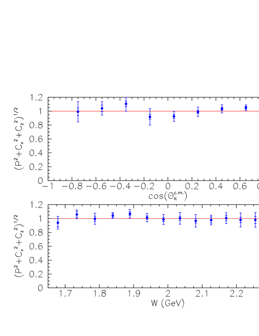
Figure 1: (color online) Magnitude of the polarization of the $\Lambda$ hyperon when averaging over all measured energies and given as a function of angle (top), and alternatively when averaged over all angles given as a function of c.m. energy (bottom). The magnitude is consistent with unity everywhere. The vector components $C_{x}$, $C_{z}$, and $P$ are discussed in the text and given in terms of helicity amplitudes in Table 1.

In this paper we will discuss some implications of these observations for other observables that have been measured already at GRAAL lleres , and LEPS zegers , or which are due to be measured at CLAS frost or ELSA bonn . We begin with a brief review of the formalism that defined the observables in a helicity basis. We will also discuss a toy model that arises under some simplifying assumptions. After discussing the measurements, we then show what conclusions may be drawn about the amplitude structure of this reaction. Finally we discuss a heuristic semi-classical picture of how hyperon polarization could arise in this reaction.

2 Formalism

2.1 Helicity basis observables

Considerable progress has been made to working out how many measurements of related observables are needed to uniquely define the four relevant amplitudes  bds ; goldstein ; worden ; tabakin ; Artru:2006xf . The intricate algebraic relations among the observables and amplitudes made this a challenging exercise. Table 1 lists the set of 16 observables relevant to this discussion. It is now known that all three of the single spin observables and the cross section must be measured, plus a judiciously-chosen set of 4 double polarization observables tabakin . The observables are given in terms of the helicity basis, in which quantization axes are taken along the momentum direction of initial and final state particles, shown as the “primed” variables in Fig. 2.

In the helicity basis, the meaning of the amplitudes is as follows. Consider $f_{0,\Lambda;\gamma,N}$ to be the amplitude that takes a photon in helicity state $\gamma$ and proton in helicity state $N$ into a final state with a spinless meson (kaon) and a recoiling baryon ($\Lambda$ hyperon) in helicity state $\Lambda$. (The notation of Goldstein et al. goldstein has been adopted.) There are eight such combinations, forming a $2\times 4$ matrix connecting the $2\times 2$ direct product space of helicities in the initial state to the 2-fold final helicity space. Parity considerations reduce the number to four, and the following naming scheme is defined:

$$f_{0,-\frac{1}{2};1,\frac{1}{2}} =N =-f_{0,\frac{1}{2};-1,-\frac{1}{2}},$$ (1)

$$f_{0,\frac{1}{2};1,-\frac{1}{2}} =D =-f_{0,-\frac{1}{2};-1,\frac{1}{2}}$$ (2)

$$f_{0,-\frac{1}{2};1,-\frac{1}{2}} =S_{1} =+f_{0,\frac{1}{2};-1,\frac{1}{2}},$$ (3)

$$f_{0,\frac{1}{2};1,\frac{1}{2}} =S_{2} =+f_{0,-\frac{1}{2};-1,-\frac{1}{2}}$$ (4)

The overall helicity flip of each of the amplitudes (defined as $|\gamma-(N-\Lambda)|$) is either none ($N$), single ($S_{1}$ and $S_{2}$) or double ($D$). It is straightforward to compute the observables in terms of these amplitudes, and the results are as summarized in Table 1. Below, we present what the CLAS measurements imply for a constraint among these amplitudes.

Observable	Helicity Representation	Beam	Target	Hyperon
Single Polarization & Cross Section
$|A|^{2}\sim d\sigma/dt$	$|N|^{2}+|S|^{2}+|S|^{2}+|D|^{2}$	-	-	-
$\Sigma\frac{d\sigma}{dt}$	$2Re(S_{1}^{*}S_{2}-ND^{*})$	linear	-	-
$T\frac{d\sigma}{dt}$	$2Im(S_{1}^{*}N-S_{2}D^{*})$	-	transverse	-
$P\frac{d\sigma}{dt}$	$2Im(S_{2}N^{*}-S_{1}D^{*})$	-	-	along $y^{\prime}$
Beam and Target Polarization
$G\frac{d\sigma}{dt}$	$-2Im(S_{1}S_{2}^{*}+ND^{*})$	linear	along $z^{\prime}$	-
$H\frac{d\sigma}{dt}$	$-2Im(S_{2}N^{*}+S_{1}D^{*})$	linear	along $x^{\prime}$	-
$E\frac{d\sigma}{dt}$	$|S_{1}|^{2}-|S_{2}|^{2}-|D|^{2}+|N|^{2}$	circular	along $z^{\prime}$	-
$F\frac{d\sigma}{dt}$	$2Re(S_{1}N^{*}+S_{2}D^{*})$	circular	along $x^{\prime}$	-
Beam and Recoil Baryon Polarization
$O_{x^{\prime}}\frac{d\sigma}{dt}$	$-2Im(S_{2}D^{*}+S_{1}N^{*})$	linear	-	along $x^{\prime}$
$O_{z^{\prime}}\frac{d\sigma}{dt}$	$-2Im(S_{2}S_{1}^{2}+ND^{2})$	linear	-	along $z^{\prime}$
$C_{x^{\prime}}\frac{d\sigma}{dt}$	$-2Re(S_{2}N^{*}+S_{1}D^{*})$	circular	-	along $x^{\prime}$
$C_{z^{\prime}}\frac{d\sigma}{dt}$	$|S_{2}|^{2}-|S_{1}|^{2}-|N|^{2}+|D|^{2}$	circular	-	along $z^{\prime}$
Target and Recoil Baryon Polarization
$T_{x^{\prime}}\frac{d\sigma}{dt}$	$2Re(S_{1}S_{2}^{*}+ND^{*})$	-	along $x^{\prime}$	along $x^{\prime}$
$T_{z^{\prime}}\frac{d\sigma}{dt}$	$2Re(S_{1}N^{*}+S_{2}D^{*})$	-	along $x^{\prime}$	along $z^{\prime}$
$L_{x^{\prime}}\frac{d\sigma}{dt}$	$2Re(S_{2}N^{*}-S_{1}D^{*})$	-	along $z^{\prime}$	along $x^{\prime}$
$L_{z^{\prime}}\frac{d\sigma}{dt}$	$|S_{1}|^{2}+|S_{2}|^{2}-|N|^{2}-|D|^{2}$	-	along $z^{\prime}$	along $z^{\prime}$

Table 1: The set of all observables for pseudoscalar meson photoproduction using helicity amplitudes. The meaning of the amplitudes $N$, $S_{1}$, $S_{2}$ and $D$ is discussed in the text. The table is adapted from Ref. bds .

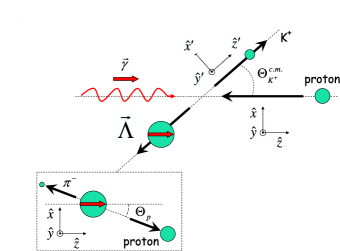
Figure 2: (color online) In the overall reaction center of mass frame, the coordinate system can be oriented along the outgoing $K^{+}$ meson $\{\hat{x}^{\prime},\hat{y}^{\prime},\hat{z}^{\prime}\}$ (helicity basis), or along the incident photon direction $\{\hat{x},\hat{y},\hat{z}\}$ ($z$-spin basis). The dotted box represents the rest frame of the hyperon, and the coordinate system used for specifying the polarization components. The short thick red arrows represent polarization vectors.

2.2 $z$-Spin Basis Model

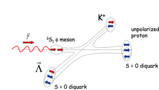
Figure 3: (color online) Quark-line picture of how full polarization of the $\Lambda$ may be achieved. An $\overline{s}s$ quark pair produced from the photon hadronizes such that the $s$ quark in the $\Lambda$ retains its full polarization after precessing due to spin-orbit or spin-spin interactions, while the $\overline{s}$ quark ends up in the spinless kaon.

In lieu of working with the four helicity amplitudes, we next consider a simplified picture in which a spin 1/2 object scatters from a spinless target schumachercxcz . The ansatz for this picture is that the incoming virtual photon fluctuates into a ${}^{3}S_{1}$ pair of $\overline{s}s$ quarks, as shown in Fig. 3. The strange quark which determines the spin of the $\Lambda$ is formed fully polarized, but during hadronization has its polarization direction precessed. This will be the case if the hadronization process is of the spin-orbit or spin-spin form, because in both quantum and classical physics such interactions preserve the magnitude of a spin, but precess its direction. In a $z$-spin basis, we can model this with two amplitudes. Let $g(\theta)$ represent the amplitude for no flip of the $s$-quark spin as a function of production angle $\theta$, and $h(\theta)$ be the amplitude that does flip the spin. The scattering matrix, $S$, that acts on an initial two-component $s$-quark spinor $\chi_{0}$ in the $z$-spin basis, has the form

$$S=\left(\begin{array}[]{cc}g(\theta)&h(\theta)e^{-i\xi}\\ -h(\theta)e^{i\xi}&g(\theta)\end{array}\right),$$ (5)

where $\xi$ is the azimuthal production angle with respect to a fixed coordinate basis. If the initial spin 1/2 density matrix is $\rho_{0}=\chi_{0}\chi_{0}^{\dagger}$, then the polarization vector $\vec{P}_{f}$ of the final state hyperon is evaluated using the spin operator $\vec{\sigma}$ via

$$\vec{P}_{f}=\frac{Tr(\rho_{0}S^{\dagger}\vec{\sigma}S)}{Tr(\rho_{0}S^{\dagger}S)}$$ (6)

In terms of the amplitudes $g$ and $h$, the polarization vector components can be written as

$$|A|^{2}= g^{*}g+h^{*}h$$ (7)

$$P_{fx}= \frac{g^{*}h+h^{*}g}{g^{*}g+h^{*}h}P_{\odot} \equiv-C_{x}P_{\odot}$$ (8)

$$P_{fy}= i\frac{g^{*}h-h^{*}g}{g^{*}g+h^{*}h} \equiv P$$ (9)

$$P_{fz}= \frac{g^{*}g-h^{*}h}{g^{*}g+h^{*}h}P_{\odot} \equiv C_{z}P_{\odot}$$ (10)

where $P_{\odot}$ is the circular polarization of the incoming photon beam. Measurement of $\vec{P}_{f}$, plus knowledge of $P_{\odot}$ and the cross section bradforddsdo then leads to a set of four observables $P,C_{x},C_{z}$, and $d\sigma/d\Omega$.

In order to make the amplitudes $g$ and $h$ dimensionless, we write the cross section as a product of a phase space factor, dimensional factors, and the magnitude of a dimensionless matrix element $A(\theta)$.

$$\frac{d\sigma}{d\Omega}=\frac{1}{4}(\hbar c)^{2}\alpha f\frac{p_{f}}{p_{i}}\frac{1}{W^{2}}|A(\theta)|^{2},$$ (11)

where $\alpha$ is the fine structure constant, and $f$ is a corresponding strong decay strength scale that was arbitrarily set equal to 1 in this calculation. $p_{f}$ and $p_{i}$ are the final and initial state momenta in the reaction center of mass frame, and $W$ is the invariant energy of the system. The combined angle-independent factors multiplying $A(\theta)$ range from 0.22 to 0.14 from low to high values of $W$ in the results discussed below. Using the four experimentally determined quantities $|A|^{2}$, $C_{x}$, $C_{z}$, and $P$, we can then solve for the magnitudes of $g$ and $h$, as well as the phase difference $\Delta\phi$ between these two complex amplitudes. The overall phase is unimportant. The result is

$$|g| = \left(\textstyle\frac{1}{2}|A|^{2}(1+C_{z})\right)^{1/2},$$ (12)

$$|h| = \left(\textstyle\frac{1}{2}|A|^{2}(1-C_{z})\right)^{1/2},$$ (13)

$$\Delta\phi = \tan^{-1}\frac{P}{C_{x}}$$ (14)

$$= \sin^{-1}\frac{P}{\sqrt{1-C_{z}^{2}}}=\cos^{-1}\frac{C_{x}}{\sqrt{1-C_{z}^{2}}}.$$ (15)

The constraint of having four observables and three unknowns allows for alternative ways of evaluating the phase difference $\Delta\phi$; we pick the one for which the propagated measurement uncertainty is most favorable.

3 Results

The CLAS measurements of $C_{x}$, $C_{z}$, and $P$ were combined to construct the magnitude of the $\Lambda$ hyperon recoil polarization when the hyperon is created from a circularly polarized photon beam. Defining the magnitude as

$$|\vec{R}_{\Lambda}|\equiv\sqrt{P^{2}+C_{x}^{2}+C_{z}^{2}},$$ (16)

it was expected that $|\vec{R}_{\Lambda}|<1$ on the physical ground that the photon spin polarization could be shared between the recoiling hyperon and the orbital angular momentum contained in the $K^{+}\Lambda$ final state. If the final state were entirely $S$-wave, as from the decay of an intermediate nucleon resonance such as the $S_{11}(1650)$, then one would expect $|\vec{R}_{\Lambda}|=1$. But there is no reason to expect the final state to be dominated by $S$-wave, and indeed most hydrodynamics models include $P$- and sometimes $D$- wave intermediate nucleon resonances. It was unexpected, therefore, when the overall average magnitude was found to be

$$\overline{R}_{\Lambda}=1.01\pm 0.01,$$ (17)

where the uncertainty is that of the weighted mean of the points in Fig. 1. The estimated systematic uncertainty is about $\pm 0.03$. A more complete presentation of the data is given in Ref bradford .

The precision of the result is limited by the CLAS data on transferred polarization $C_{x}$ and $C_{z}$. The CLAS data for induced $P$ have recently be seen to be in excellent agreement with results from GRAAL lleres . But incorporating those values for $P$ into the calculation of $\vec{R}_{\Lambda}$ does not lead to smaller uncertainties. Thus, a new experiment for $C_{x}$ and $C_{z}$ would be needed to improve the overall precision of $\vec{R}_{\Lambda}$.

In electroproduction, the $K^{+}\Lambda$ final state has been studied in the range $0.3<Q^{2}<1.5$ (GeV/c)², integrated over all kaon production angles carman . The electron beam was longitudinally polarized, allowing extraction of the spin transfer to the hyperon in a manner analogous to the photoproduction analysis. The hyperon spin was found to be dominantly in the direction of the photon momentum, that is, along the $z$ axis of virtual photon. The phenomenology away from $Q^{2}=0$ was thus seen to be quite similar to the photoproduction result emphasized in this paper.

The other recent measurements of polarization observables were for the beam spin asymmetry, $\Sigma$, using linearly polarized photons. Measurements from threshold up to 1.5 GeV photon energy made at GRAAL lleres are in good agreement with measurements made at LEPS/SPring8  zegers at energies from 1.5 to 2.4 GeV. The observable $\Sigma$ can not be predicted on the basis of the constraint implied by the CLAS results, unfortunately, as discussed below.

3.1 Helicity Amplitudes Constraint

Combining the experimental result discussed above with the helicity amplitude relations summarized in Table 1, we can derive an expression relating the helicity amplitudes. We find that

$$S_{1}S_{2}=ND.$$ (18)

That is, the product of the two single-helicity-flip amplitudes is equal to the product of the the no-flip and the double-flip amplitudes. This is the empirical constraint implied by the data. The next step would be to make predictions for what this constraint imposes on observables that have been (or soon will be) measured, such as $\Sigma$, $O_{x}$, $O_{z}$, or $T$  lleres2 ; althoff . However, this seems to be fruitless based on this constraint alone. Note that Eq. 18 is for products of amplitudes, while the observables are constructed out of bilinear products of an amplitude and an complex conjugate amplitude. In an earlier paper schumachercxcz we speculated that if a linearly polarized beam were used to measure $O_{x}$ and $O_{z}$, then in combination with $P$ one might again find a magnitude of the polarization vector to be unity, that is,

$$O_{x}^{2}+O_{z}^{2}+P^{2}=1.$$ (19)

But this does not follow; the constraint given by Eq. 18 does not lead to this conclusion. The conjecture given by Eq. 19 may or may not be true, but the information in hand does not predict either one outcome or the other. There are results coming from GRAAL for these observables lleres2 , and so we may have some insight in this area soon.

3.2 $z$-Spin Basis Model

In terms of the two-amplitude model discussed in the previous section, Fig. 4 shows the squared-magnitudes of the amplitudes $g(\theta)$ and $h(\theta)$. The squares are shown since, as seen in Eq. 13, $|h|^{2}$ can be negative in regions where the $C_{z}$ measurement exceeds the physical limit of $C_{z}=1$ due to fluctuations. This representation amplifies the main message: the non-flip amplitude $g$ is the dominant one at forward angles, while the spin-flip amplitude $h$ plays a significant role mainly at higher energies in the backward hemisphere. This reaction is occurring very far from the limit of quark helicity conservation, and is indeed much closer to the limit of $s$-channel spin conservation at the baryon level.

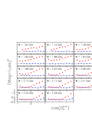
Figure 4: (color online) The squared magnitudes of the spin non-flip $|g|^{2}$ (red circles) and spin flip $|h|^{2}$ (blue triangles) amplitudes for the reaction $\gamma+p\rightarrow K^{+}+\Lambda$. Each panel for a bin in $W$ is given as a function of c.m. kaon production angle. Note the displaced zero on the vertical axis, and that the points are slightly shifted in angle to avoid overlaps.

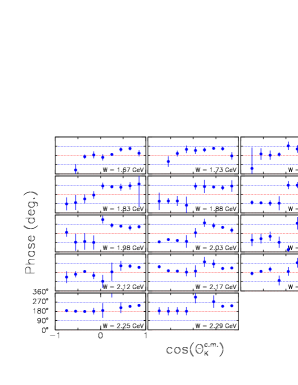
Figure 5: (color online) The phase difference of the spin non-flip $g$ and spin flip $h$ amplitudes, $\Delta\phi=\phi_{g}-\phi_{h}$, for the reaction $\gamma+p\rightarrow K^{+}+\Lambda$. The binning and the various $W$ panels match those of the previous figure.

The relative phase, $\Delta\phi=\phi_{g}-\phi_{h}$ is shown in Fig. 5. For each datum, the form of Eq. 15 that resulted in the smallest propagated error was adopted. Qualitatively, we see that with increasing $W$ the relative phase evolves from being nearer $\pm\pi/2$ to being nearer to $\pi$. The discontinuities seen near $W=2.00$ GeV arise when the value of $P$ passes through zero while $C_{x}$ remains small and negative. The trends are of limited statistical significance, unfortunately. There are no model-based expectations available with which to compare the results of this simple two-amplitude model. It’s main value is to underscore the dominance of the spin non-flip nature of this reaction.

3.3 Semi-Classical Model

In a magnetic field, the expectation value of a quantum mechanical spin with magnetic moment $\vec{\mu}$ evolves in time the same way as a classical “spin” angular momentum vector does merz . In a constant magnetic field, a spin $\vec{\mu}$ will precess at its Larmor frequency due to a torque $\vec{\mu}\times\vec{B}$. Starting from this observation, one can build a qualitative picture of the reaction mechanism discussed in this paper. We take literally the head-to-tail triplet orientation of the initial state configuration of a virtual $\overline{s}s$ quark pair shown in Fig. 3. Their spin-spin dipole interaction is taken to be of the classical form $\vec{\mu}\cdot\vec{B}$, where the field of one dipole at the location of the other at relative location $\vec{r}$ is $\vec{B}=\frac{1}{r^{3}}\left[3(\vec{\mu}\cdot\hat{r})\hat{r}-\vec{\mu}\right]$. The strength scale of the field is not that of the electromagnetic interaction, since we expect the color-magnetic (gluonic) force to be dominant. Indeed, in the result shown below the value of the effective fine structure constant $\alpha_{eff}$ was increased by a factor of 30 to get qualitatively reasonable behavior. The dipole strength of the strange quark was written as $|\vec{\mu}|=\alpha_{eff}\frac{(\frac{2}{3}e)\hbar}{2m_{s}}\sqrt{\frac{1}{2}(\frac{1}{2}+1)}$ where the strange quark mass, $m_{s}$, was taken as 150 MeV. The spacing of the initial-state quarks was set to half the wavelength of the incoming photon in the overall c.m. frame.

As long as the quark pair remains axially aligned there is no dipole-dipole torque. But then one considers the motional (color-) magnetic field of a proton charge distribution as it interacts with the quark pair. Modeling a proton as a spinless charge distribution with a root-mean-square radius of $R_{rms}=0.86$ fm, the collision of moving proton and quark magnetic dipoles first precesses the dipoles off their alignment axis. The spin-spin interaction then serves to precess the quarks further. The semi-classical model system can be allowed to interact in this way for some characteristic “hadronization time” which was taken to be 1 fm/$v_{cm}$, where $v_{cm}$ is the speed of the quark pair in the overall c.m. system. After this “hadronization time” the strange quark is presumed to have formed a $\Lambda$ hyperon, to have moved out of range of the strong force, hence freezing its orientation. The production-angle dependence of the model is built into a mapping of the classical collisional impact parameter, $b$, onto scattering angle. Parameter $b$ affects the motional (color-) magnetic field and hence degree of quark precession. We used a Rutherford-like mapping $\theta=2\tan^{-1}(2b/r_{0})$ where $r_{0}=R_{rms}/\sqrt{12}$.

A numerical simulation was developed to compute the resultant hyperon polarization as a function is scattering angle. The result is shown in Fig. 6 for the typical case of $W=2.0$ GeV. It was remarkably simple to find a set of model parameters that mimic the observed phenomenology. That is, $C_{z}$ is large and positive, meaning that the strange quark spin was not much perturbed from its initial direction. $C_{x}$ remains small and negative across the range of production angles. Finally, the out-of-plane polarization component $P$ is negative at forward production angles and positive and backward production angles. This is what is seen in the measurements bradford . By construction, $\vec{R}_{\Lambda}=1$ in this model.

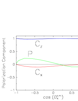
Figure 6: (color online) Results of a semi-classical model of $\Lambda$ hyperon polarization for a total c.m. energy of $W=2$ GeV. The three projections of the polarization vector are shown as a function of kaon production angle. The model is based on the spin-spin and spin-orbit interaction of an $\overline{s}s$ quark pair and the (color-) magnetic field of a proton charge distribution.

We cannot expect this semi-classical picture to be developed into a realistic model of this reaction. There are many free parameters in this model that cannot be connected in any useful way to measured properties of the particles involved. Its main value is to offer a possible physical explanation of how, classically, a spin can be created and made to partially point “out of plane” with respect to the beam polarization axis. It offers heuristic support to the hypothesis that the observed $\Lambda$ polarization arises from the creation of a strange quark pair in a triplet state that is acted upon by a spin-magnitude preserving color-magnetic hadronization process.

4 Further Discussion and Conclusions

The CLAS results on $C_{x}$, $C_{z}$, and $P$ have recently been satisfactorily fit in coupled-channel baryon-resonance model by the Bonn-Gachina group bg . In that model, the quark-level dynamics advocated here are not relevant, but instead a well-defined set of $s$-channel isobars are made to interfere to explain the $K^{+}\Lambda$ results, together with a number of other reaction channels. A new $P_{13}$ resonance near 1860 MeV was introduced to fit the $C_{x}$ and $C_{z}$ results. Their approach could be the most profitable one for explaining the broad array of reaction channels in terms of a unified model framework. But it is worth keeping in mind that the apparently “simple” result that $|\vec{R}_{\Lambda}|=1$ across energy and angle may signal a more fundamental dynamic about how the reaction mechanism proceeds, something other than the interference of multiple baryon resonances.

In this discussion we have ignored the less-precise data available for the polarization components of the $\Sigma^{0}$ hyperon bradford ; mcnabb . In the flavor SU(3) quark model, the magnetic moment of the $\Sigma^{0}$ is opposite to that of the $\Lambda$, and indeed it is seen that observables $P$ for the two hyperons are roughly opposites of each other. The $C_{z}$ and $C_{z}$ behaviors are not similar, but the data are consistent with the requirement that $C_{z}$ for the $\Sigma^{0}$ goes to unity at forward angles. The phenomenological models discussed in this paper have yet to be adapted to the $\Sigma^{0}$ case.

We have discussed the observables available in hyperon photoproduction, in particular $K^{+}\Lambda$ photoproduction from the proton, in light of recent measurements by the CLAS collaboration of $C_{x}$, $C_{z}$, and $P$. In the helicity basis, one obtains a product relationship among the four amplitudes. By itself, this empirical constraint does not lead algebraically to predictions for the other spin observables. But the observation that the $\Lambda$ hyperon is produced fully polarized from a photon of definite helicity suggests a physical picture in which a virtual $s$ quark is created with full polarization, and that the hadronization process preserves the full magnitude but not the direction. In a two-amplitude model in a $z$-spin basis, the result says that the spin non-flip amplitude is by far the dominant one over the spin-flip amplitude. We computed the magnitudes and relative phase of these amplitudes, which showed smooth trends across energy and production angle. A semi-classical model of spin-spin and spin-orbit interactions of (color-) magnetic moments with their associated fields was seen to reproduce the qualitative features of the data. Further work to interpret these results is needed, as well as additional constraints from other observables.

In closing, it is encouraging to note that experimental work at CLAS frost , Crystal Barrel/TAPS at Bonn bonn , and GRAAL lleres2 is underway to measure additional spin observables in hyperon photoproduction and related reactions in pseudoscalar meson photoproduction. Therefore, progress in unraveling the amplitude-level structure of these reactions can be expected. It will be interesting to see to what extent the physical mechanisms discussed in this paper will be supported.

References

- (1) M. Jacob and G. C. Wick, Annals of Physics 7, (1959) 404.
- (2) I. S. Barker, A. Donnachie, and J. K. Storrow, Nucl. Phys. B95, (1975) 347.
- (3) R. Bradford, R. A. Schumacher et al. [CLAS Collaboration], Phys. Rev. C 75, (2007) 035205.
- (4) J. W. C. McNabb, R. A. Schumacher, L. Todor, et al. [CLAS Collaboration], Phys. Rev. C 69, (2004) 042201(R).
- (5) R. A. Schumacher, HYP2006 Proceedings, to be published by Springer Verlag; arXiv:nucl-ex/0611035.
- (6) A. Lleres et al. [GRAAL Collaboration], Eur. Phys. J. A 31, (2007) 79.
- (7) R. G. T. Zegers et al. [LEPS Collaboration], Phys. Rev. Lett. 91, (2003) 092001.
- (8) F. J. Klein, Proc. of the Workshop on the Physics of Excited Nucleons, “NStar2005”, Tallahassee, FL, Oct. 2005, S. Capstick, V. Crede, P. Eugenio, Eds., World Scientific, 159 (2006); arXiv:nucl-ex/0602004 (2006).
- (9) H. Schmieden, “Physics at ELSA”, these proceedings.
- (10) G. R. Goldstein, J. F. Owens, J. P. Rutherfoord, M. J. Moravcsik, Nucl. Phys. B80 (1974) 164.
- (11) R. P. Worden, Nucl. Phys. B37, (1972) 253.
- (12) Wen-Tai Chiang and Frank Tabakin, Phys. Rev. C 55, (1997) 2054.
- (13) X. Artru, J. M. Richard and J. Soffer, Phys. Rev. C 75, (2007) 024002.
- (14) R. Bradford, R.A. Schumacher, J. W. C. McNabb, L. Todor, et al. [CLAS Collaboration], Phys. Rev. C 73 (2006) 035202.
- (15) D. S. Carman et al. [CLAS Collaboration], Phys. Rev. Lett. 90, 131804 (2003). See also P. Ambrozewicz et al. [CLAS Collaboration], Phys. Rev. C 75, (2007) 045203.
- (16) A. Lleres (GRAAL Experiment), private communication.
- (17) K. H. Althoff et al. Nucl. Phys. B137, (1978) 269.
- (18) See for example Eugen Merzbacher, Quantum Mechanics, 2nd Ed. (John Wiley and Sons, New York, 1970) p281.
- (19) These proceedings; see also: A. V. Sarantsev, V. A. Nikonov, A. V. Anisovich, E. Klempt, and U. Thoma, Eur. Phys. J. A 25, 441 (2005), and references therein.