Genericity of blackhole formation in the gravitational collapse of homogeneous self-interacting scalar fields

Abstract.

The gravitational collapse of a wide class of self-interacting homogeneous scalar fields models is analyzed. The class is characterized by certain general conditions on the scalar field potential, which, in particular, include both asymptotically polynomial and exponential behaviors. Within this class, we show that the generic evolution is always divergent in a finite time, and then make use of this result to construct radiating star models of the Vaidya type. It turns out that blackholes are generically formed in such models.

1. Introduction

Scalar fields attracted a great deal of attention in cosmology and in relativistic astrophysics in the last twenty years. It is, indeed, worth mentioning the fundamental role that they play in modeling the early universe and, on the other hand, the relevance of the self-gravitating scalar field model as a test-bed for the Cosmic Censorship conjecture, that is, whether the singularities which form at the end state of the gravitational collapse are always covered by an event horizon, or not [8, 17]. In particular, in an important series of papers, Christodolou studied massless scalar field sources minimally coupled to gravity. For this very special case the formation of some naked singularities has been shown, but it has been also shown that such singularities are non generic with respect to the choice of the initial data [3, 4].

The massless scalar field is a useful model in studies of gravitational collapse since its evolution equation in absence of gravity - the massless Klein-Gordon equation on Minkowski spacetime - is free of singular solutions. However, of course, the general case in which the field has non-zero self-interaction potential (which of course include the massive scalar field as a quadratic potential) is worth inspecting from the theoretical point of view. Further to this, in recent years, interest in models with non vanishing potentials aroused from string theory, since, for instance, dimensional reduction of fundamental theories to four dimensions typically gives rise to self-interacting scalar fields with exponential potentials, coupled to four-dimensional gravity. In this context, the case of potentials which have a negative lower bound plays a special role, since such potentials generate the anti De Sitter space as equilibrium solutions [14, 15].

As a consequence of their ”fundamental” origin, exponential potentials have been widely considered in the cosmologically-oriented literature (see [25] and references therein) also with the aim of uncovering possible large-scale observable effects [6, 20, 21, 26]. A few examples of non trivial potentials (to be discussed in full details in the sequel) have been studied in the gravitational collapse scenario as well. In these papers formation of naked singularities has been found [9, 12].

So motivated, in the present paper we study the dynamical behavior of FRW (spatially flat) scalar field models, imposing only very general conditions on the scalar field potential; our hypotheses essentially reduce to ask the potential to be bounded from below and divergent when the field diverges. The evolution of collapsing solutions or, equivalently, time backwards expanding solutions, has been studied previously in the literature mainly making use of dynamical system approaches. From this point of view Foster’s work is worth noticing; indeed, in [7] existence of past singularities of expanding, spatially flat cosmologies are found in terms of sufficient conditions on the (nonnegative) potential $V(\phi)$ – in particular, the proof relies on the existence of a coordinate transformation that brings $[\phi_{0},+\infty[$ in $]0,\epsilon]$ , and satisfies some other regularity conditions together with the transformed potential (see [7, Definition 2]). In these cases, the behavior is proved to be essentially similar to the behavior in the massless case, and so a past singularity exists and it is stable with respect to the choice of the data.

Other worth-mentioning works are those related to the case of non-minimal coupling, such as [2], in which flat FRW model are studied using conformal transformations that bring the models into the standard form, and [5], where singularity formation for non minimal coupling models is analyzed for some specific form of the potential.

As mentioned above, in this paper we consider a class of potentials $\mathfrak{C}$ which is quite more general with respect to those previously considered. In particular, we weaken assumptions about the behavior of the potential at infinity (which are necessary in the dynamical systems approach) thanks to an accurate use of the Implicit Function Theorem. Indeed a suitable estimate of the involved neighborhoods is used to obtain a result of existence, uniqueness, and instability of solution for a particular kind of ordinary differential equation of first order to which the standard theory does not apply straightforwardly (Theorem 3.6). Another key difference with previously published results is that the potentials may assume negative values. Non negativity of the potential means that the total energy of the scalar field has a positive lower bound (using this constraint many results for scalar field cosmologies have been actually found [7, 18, 19, 22, 23, 24]; see also [11]); however, in many issues and especially when string theory comes into play, it becomes relevant to inspect spacetimes in which the potential still has a lower bound but this bound is negative; under certain conditions indeed, potentials of this kind generate solutions with positive total energy [16]. Since, in particular , a constant negative potential generates an ”equilibrium” state which is just the Anti de Sitter solution, within this framework models which are asymptotically anti-De Sitter can be inspected [11, 14, 15].

Within the class $\mathfrak{C}$ of potentials (to be defined in precise technical terms in the section below) we prove that - except for a zero measure set of initial data - all the solutions become singular in a finite time. Considering such solutions as sources for models of collapsing objects (with generalized Vaidya solutions as the exterior) we study the nature - blackhole or naked singularity - of such objects. It turns out that, except possibly for a zero-measure set of initial data, all these ”scalar field stars” collapse to black holes. It follows that the existing examples of naked singularities which occur in the literature must be non-generic within the set of possible solutions, and indeed we show in details how this occurs.

Homogeneous scalar field models with self-interacting potentials thus respect the weak cosmic censorship hypothesis, at least for a wide class of potentials. Of course, however, the problem of extending this result to the non-homogeneous case remains open.

2. Collapsing models

We are going to consider here homogeneous, spatially flat spacetimes

(2.1) $$g=-\mathrm{d}t\otimes\mathrm{d}t+a^{2}(t)\left[\mathrm{d}x^{1}\otimes\mathrm{d}x^{1}+\mathrm{d}x^{2}\otimes\mathrm{d}x^{2}+\mathrm{d}x^{3}\otimes\mathrm{d}x^{3}\right]$$

where gravity is coupled to a scalar field $\phi$, self-interacting with a scalar potential $V(\phi)$. Assigning this function is equivalent to assign the physical properties of the matter source, and thus the choice of the potential can be seen as a choice of the equation of state for the matter model. Therefore, as occurs in models with ”ordinary” matter (e.g., perfect fluids), the choice of the ”equation of state” must be restricted by physical considerations. Stability of energy, in particular, requires the potential to have a lower bound. We shall thus consider here potentials of class $C^{2}(\mathds{R})$ bounded from below; the lower bound of the potential need not be positive however, so that class of solutions which include AdS minima can be considered. Further, we need a set of technical assumptions.

We say that $V$ belongs to the set $\mathfrak{C}$ if the following conditions are satisfied:

A1) (Structure of the set of critical points) The critical points of $V$ are isolated and they are either minimum points or non-degenerate maximum points

A2) (Existence of a suitable bounded ”sub-level” set) There exists $\alpha<\beta\in\mathds{R}$ such that

$$\phi\geq\beta\Longrightarrow V^{\prime}(\phi)>0,\,\phi\leq\alpha\Longrightarrow V^{\prime}(\phi)<0.$$

Moreover, setting $V_{*}=\max_{[\alpha,\beta]}V$, it is

$$\lim_{\phi\rightarrow-\infty}V(\phi)>V_{*},\,\lim_{\phi\rightarrow+\infty}V(\phi)>V_{*}.$$

A3) (Growth condition) The function defined in terms of $V$ and its first derivative $V^{\prime}$ as

(2.2) $$u(\phi):=\frac{V^{\prime}(\phi)}{2\sqrt{3}V(\phi)},$$

satisfies to

(2.3) $$\limsup_{\phi\to\pm\infty}|u(\phi)|<1,$$

(2.4) $$\exists\lim_{\phi\to\pm\infty}{u^{\prime}(\phi)}\,(=0).$$

We stress that the set $\mathfrak{C}$ defined in terms of the above conditions is sufficiently large to contain all the potentials which have been considered in physical applications so far. For instance, it contains the standard quartic potential ($V(\phi)=\frac{1}{2}m^{2}\phi^{2}+\lambda^{2}\phi^{4}$) and, more generally, all the potentials bounded from below whose asymptotic behavior is polynomial (i.e. $\phi^{2n}$ for $|\phi|\to\infty$, $n\geq 1$).

Once a potential has been chosen, the Einstein field equations allow, in principle, to obtain the dynamics of the coupled system composed by the field and the metric. These equations are given by

(2.5a) $$(G^{0}_{0}=8\pi T^{0}_{0}):\qquad-\frac{3\dot{a}^{2}}{a^{2}}=-(\dot{\phi}^{2}+2V(\phi)),$$

(2.5b) $$(G^{1}_{1}=8\pi T^{1}_{1}):\qquad-\frac{\dot{a}^{2}+2a\ddot{a}}{a^{2}}=(\dot{\phi}^{2}-2V(\phi)),$$

the Bianchi identity is of course, due to the Noether theorem, equivalent to the equation of motion for the field:

(2.6) $$T^{\mu}_{\,\,0;\mu}=-2\dot{\phi}\left(\ddot{\phi}+V^{\prime}(\phi)+3\frac{\dot{a}}{a}\dot{\phi}\right)=0.$$

Denoting the energy density of the scalar field by

(2.7) $$\epsilon=\dot{\phi}^{2}+2V(\phi),$$

We will actually consider the following system:

(2.8a) $$\left(\frac{\dot{a}}{a}\right)^{2}={\frac{\epsilon}{3}}.$$

(2.8b) $$\ddot{\phi}+V^{\prime}(\phi)=-3\frac{\dot{a}}{a}\,\dot{\phi},$$

Of course, it is mandatory to extract the square root in the first equation. Since we are considering the collapsing model we choose $\dot{a}$ to be negative and therefore our final system is composed by

(2.9a) $$\frac{\dot{a}}{a}=-\sqrt{\frac{\epsilon}{3}}.$$

(2.9b) $$\ddot{\phi}+V^{\prime}(\phi)=\sqrt{3}\sqrt{\epsilon}\,\dot{\phi}.$$

Let us observe that, using (2.7) and (2.9b), the following relation can be seen to hold:

(2.10) $$\dot{\epsilon}=2\sqrt{3}\sqrt{\epsilon}\,\,\dot{\phi}^{2},$$

that is $\epsilon(t)$ is monotone. Observe that the two cases - expansion and collapse - are connected by the fact that, in the expanding case, there might be the possibility of reaching a vanishing value of $\epsilon$ in a finite time $t_{0}$. If this occurs, the model will be ruled from $t_{0}$ onward by the equations for the collapsing situation. Actually, it will be proved that all such solutions are divergent at some finite time for almost every choice of the initial data, thus yielding a singularity as well.

In what follows, we are going to focus on solutions of the equations (2.8a)–(2.8b) – or, better, (2.9a)–(2.9b). Actually, it can be proved [10] that, if $a\neq 0$ for all $t\geq 0$ and $(a,\phi)$ are $\mathcal{C}^{2}$ functions that solve (2.5a)–(2.5b) (with a non-constant $\phi(t)$) then they are solutions of (2.8a)–(2.8b) as well. To prove the converse, it suffices to derive (2.8a) w.r.t. time and use (2.8b) to deduce that if (in some interval $[a,b]$), $\dot{a}$ is not identically zero – that is, $\epsilon\neq 0$ – then solutions of (2.8a)–(2.8b) are also solutions of (2.5a)–(2.5b). Finally, the unique case in which $\epsilon(t)=0,\forall t>0$ and the Einstein Field Equations are satisfied is given by the trivial solution $a(t)=a_{0}$, $\phi(t)=\phi_{0}$, with $V(\phi_{0})=0$.

3. Qualitative analysis of the collapsing models

The aim of the present section is to study the qualitative behavior of the solutions of (2.9a)–(2.9b) whenever $V\in\mathfrak{C}$. The initial data (on $t=0$, say) for the system can be fully characterized in terms of the values of the scalar field $\phi_{0}=\phi(0)$ and of its first derivative. In what follows we will be mainly interested in constructing models of collapsing object and therefore we consider only solutions which satisfy the weak energy condition on the initial data surface. Therefore, we assume

(3.1) $$\epsilon_{0}=\epsilon(0)=\dot{\phi}^{2}(0)+2V(\phi(0))\geq 0.$$

Given a solution $\phi(t)$, let $\mathds{I}\subseteq[0,+\infty)$ be the maximal right neighborhood of $t=0$ where the solution is defined, and call $t_{s}=\sup\mathds{I}$. The main result of this section is that the solution $\phi(t)$ diverges in a finite time for almost every choice of the initial data satisfying (3.1), that is $t_{s}$ is finite for almost all solutions. This result will in turn allow us (next section) to construct models of collapsing objects by matching these solutions with suitable Vaidya metrics.

To proceed further, we start by considering only data such that $\epsilon_{0}$ is ”sufficiently large”, more precisely

(3.2) $$\epsilon_{0}>2V^{*},$$

where, for each choice of the potential $V$ in $\mathfrak{C}$, the constant $V^{*}$ is the chosen as the same which appears in (A2). Once the result will be proven for these data, we will extend its validity by removing the restriction (3.2).

We start our study with the following lemma.

Lemma 3.1.

If $\phi(t)$ is bounded, also $\dot{\phi}(t)$ is bounded, and $t_{s}=+\infty$.

Proof.

Let $K$ a bounded set such that $\phi(t)\in K,\,\forall t\in\mathds{I}$, and argue by contradiction, assuming $\dot{\phi}$ not bounded, and supposing that $\sup_{\mathds{I}}\dot{\phi}(t)=+\infty$ – the same argument can be used if $\dot{\phi}$ is unbounded only below. Let $\bar{t}$ such that

$$\dot{\phi}(\bar{t})>\frac{\sup_{K}V^{\prime}(\phi)}{\sqrt{3\epsilon_{0}}},$$

therefore (2.9b) implies that $\ddot{\phi}(\bar{t})>0$, and this means that $\dot{\phi}$ is increasing in $\bar{t}$, so (2.9b) shows that $\ddot{\phi}\geq 0,\,\forall t\geq\bar{t}$, and then $\dot{\phi}$ is eventually increasing, namely $\lim_{t\to t_{s}}\dot{\phi}(t)=+\infty$. This shows that $t_{s}<+\infty$, otherwise it would be $\phi(t)-\phi_{0}=\int_{0}^{t}\dot{\phi}(\tau)\,\mathrm{d}\tau$, which would diverge as $t\to+\infty$. Then $t_{s}\in\mathds{R}$.

With the position

$$\lambda(t)=\frac{1}{\dot{\phi}(t)},$$

equation (2.9b) implies

$$\dot{\lambda}(t)=\frac{V^{\prime}(\phi(t))}{\dot{\phi}(t)^{2}}-\sqrt{3}\sqrt{1+\frac{2V(\phi(t))}{\dot{\phi}(t)^{2}}}\xrightarrow{t\to t_{s}^{-}}-\sqrt{3},$$

and then $\lambda(t)$, near $t=t_{s}$, behaves like $\sqrt{3}(t_{s}-t)$. Since $\dot{\phi}(t)$ positively diverges, $\lim_{t\to t_{s}}\phi(t)=\phi^{*}$ exists, and is finite since $\phi(t)$ is bounded by hypothesis. But the quantity

$$\phi(t)-\phi^{*}=\int_{t_{s}}^{t}\dot{\phi}(\tau)\,\mathrm{d}\tau=\int_{t_{s}}^{t}\frac{1}{\lambda(\tau)}\,\mathrm{d}\tau$$

diverges, which is absurd. This shows that $\dot{\phi}(t)$ must be bounded too.

To prove that $t_{s}=+\infty$, we proceed again by contradiction. Let $t_{k}\to t_{s}$ be a sequence such that the sequence $(\phi(t_{k}),\dot{\phi}(t_{k}))$ converges to a finite limit $(\phi_{*},\dot{\phi}_{*})$. Solving the Cauchy problem (2.9b) with initial data $(\phi_{*},\dot{\phi}_{*})$ shows that the solution $\phi(t)$ is $\mathcal{C}^{1}$, the solution could be prolonged on a right neighborhood of $t_{s}$. ∎

Proposition 3.2.

The function $\phi(t)$ is unbounded.

Proof.

Let by contradiction $\phi(t)$ be bounded. Then, by Lemma 3.1, $|\dot{\phi}(t)|\leq M$ for a suitable constant $M$, and $t_{s}=\sup\mathds{I}=+\infty$. In particular $V(\phi(t)),V^{\prime}(\phi(t)),\epsilon(t),\ddot{\phi}(t)$ are bounded also. Then Lemma A.1 in Appendix A says that $\lim_{t\to+\infty}\dot{\phi}(t)=0$, that implies $\lim_{t\to+\infty}2V(\phi(t))=\lim_{t\to+\infty}\epsilon(t)\geq\epsilon_{0}>2V_{*}$, and so $V(\phi(t))>V_{*}$ for any $t$ sufficiently large. Then, by assumption A2), for large $t$, $\phi(t)$ moves outside the interval $[\alpha,\beta]$ described in assumption A2), namely in a region where $V$ is invertible. Since $V(\phi(t))$ converges this happen also for $\phi(t)$ which converges to a point $\phi_{*}\not\in]\alpha,\beta[$. Then by (2.9b), $\ddot{\phi}(t)\to-V^{\prime}(\phi_{*})\neq 0$ (since $\dot{\phi}(t)\rightarrow 0$), that is absurd. Then $\limsup_{t\to t_{s}}|\phi(t)|=+\infty$. ∎

We have shown that $\phi(t)$ is not bounded. Now we want to show that, actually, $\phi(t)$ monotonically diverges in the approach to $t_{s}$.

Remark 3.3.

We observe that the quantity

(3.3) $$\rho(t):=\frac{2V(\phi(t))}{\dot{\phi}(t)^{2}},$$

satisfies the equation

(3.4) $$\dot{\rho}=2\sqrt{3}\dot{\phi}\,\rho\sqrt{(1+\rho)}\left(u(\phi)\sqrt{1+\rho}-\mathrm{sgn}\,(\dot{\phi})\right).$$

Proposition 3.4.

Let $V\in\mathfrak{C}$, and let $\phi:\mathds{I}\subseteq\mathds{R}\to\mathds{R}$ the solution of (2.9b). Then $\dot{\phi}(t)$ is eventually nonzero, and

$$\lim_{t\to\sup\mathds{I}}|\phi(t)|=+\infty.$$

Proof.

Note that $\dot{\phi}(t)=0$ imply $V(\phi(t))=\frac{1}{2}\epsilon(t)\geq\frac{1}{2}\epsilon_{0}>V_{*}$, so $\phi\not\in[\alpha,\beta]$. Moreover if $\phi(t)>\beta$ , it is $V^{\prime}(\phi(t))>0$ so $\ddot{\phi}(t)<0$, while if $\phi(t)<\alpha$ it is $\ddot{\phi}(t)>0$, Therefore if by contradiction, $\dot{\phi}(t)=0$ for infinitely many values of $t$, we see that $\phi(t)$ crosses the interval $[\alpha,\beta]$ infinitely many times.

Then there exist sequences $\sigma_{k}<\tau_{k}$ going to $t_{s}$ such that

$$\phi(\sigma_{k})=\alpha,\qquad\phi(\tau_{k})=\beta,\qquad\phi([\sigma_{k}\tau_{k}])\subseteq[\alpha,\beta],$$

and

$$\beta-\alpha=\phi(\tau_{k})-\phi(\sigma_{k})=\int_{\sigma_{k}}^{\tau_{k}}\dot{\phi}(t)\mathrm{d}t\leq M(\tau_{k}-\sigma_{k}),$$

and so $\tau_{k}-\sigma_{k}\geq\tfrac{\beta-\alpha}{M}$. Moreover, since $\phi([\sigma_{k},\tau_{k}])\subseteq[\alpha,\beta]$ it is

$$\epsilon_{0}\leq\epsilon(t)=(\dot{\phi}(t))^{2}+2V(\phi(t))\leq(\dot{\phi}(t))^{2}+2V_{*}$$

for any $t\in[\sigma_{k},\tau_{k}]$. Then

$$(\dot{\phi}(t))^{2}\geq\epsilon_{0}-2V_{*}>0$$

for any $t\in[\sigma_{k},\tau_{k}]$.

Therefore, by (2.10),

$$\sqrt{\epsilon(\tau_{k})}-\sqrt{\epsilon(\sigma_{k})}=\int_{\sigma_{k}}^{\tau_{k}}\frac{\dot{\epsilon}}{2\sqrt{\epsilon}}\,\mathrm{d}t=\sqrt{3}\int_{\sigma_{k}}^{\tau_{k}}\dot{\phi}^{2}\,\mathrm{d}t\geq(\epsilon_{0}-2V_{*})\sqrt{3}(\tau_{k}-\sigma_{k})\geq(\epsilon_{0}-2V_{*})\sqrt{3}\tfrac{\beta-\alpha}{M},$$

and then $\epsilon(t)$ must diverge.

Now, recalling (2.3), let $\theta>0$ be a sufficiently small constant, and let $r_{k}\to t_{s}$ a sequence such that $\phi(r_{k})=\bar{\phi}$, with $u(\phi)\leq 1-\theta$ as $\phi\geq\bar{\phi}$. Then $\dot{\phi}(r_{k})^{2}=\epsilon(r_{k})-2V(\bar{\phi})\to+\infty$. Let us suppose that $\dot{\phi}(r_{k})$ is unbounded above – analogously one can argue if it is only unbounded below. Up to subsequences, we can suppose that $\dot{\phi}(r_{k})$ positively diverges. Moreover, recalling (3.3), $\rho(r_{k})\to 0$ and then, if $k$ is sufficiently large,

$$|\rho(r_{k})|<\left(\frac{1}{1-\theta}\right)^{2}-1,$$

so that, since $\phi(r_{k})=\bar{\phi}$ and $u(\bar{\phi})\leq 1-\theta$, we have

$$u(\phi(r_{k}))\sqrt{1+\rho(r_{k})}-1<0.$$

Then, $\dot{\rho}(r_{k})<0$, that is $\rho(t)$ is decreasing at $r_{k}$. But we can observe that $\phi(t)$ is increasing in $r_{k}$, ensuring $u(\phi(t))<1-\theta$, and so, in a right neighborhood of $r_{k}$,

$$u(\phi(t))\sqrt{1+\rho(t)}-1<(1-\theta)\sqrt{1+\rho(t)}-1$$

that is decreasing. We conclude that the function $\rho(t)=\tfrac{2V(\phi(t))}{\dot{\phi}^{2}(t)}$ decreases for $t>r_{k}$, until $t$ equals a local maximum $t_{k}$, where $\dot{\phi}$ vanishes. Then there exists $\kappa>0$ such that $2V(\phi(t))\leq\kappa\dot{\phi}(t)^{2}$ until $t$ equals a local maximum $t_{k}$. But this would imply $\epsilon(\phi(t_{k}))=0$, getting a contradiction. Then $\dot{\phi}$ is eventually non zero. This implies that there exists $\lim\limits_{t\rightarrow+\infty}|\phi(t)|$ so, by Proposition 3.2, it is $+\infty$. ∎

We have shown so far that $\phi(t)$ diverges, as $t$ approaches $t_{s}=\sup\mathds{I}$. In the following, we will show that $t_{s}\in\mathds{R}$ for almost every solution, in the sense that there exists a set of initial data, whose complement has zero Lebesgue measure, such that the solution is defined until a certain finite comoving time $t_{s}$ (depending on the data).

Henceforth we will suppose (just to fix ideas) $\phi(t)$ positively diverging and $\dot{\phi}(t)>0$ $\forall t\geq\bar{t}$. Then, in the interval $[\bar{t},+\infty)$, $\rho$ can be seen as a function of $\phi$, that satisfies by (3.4) the ODE

(3.5) $$\frac{\mathrm{d}\rho}{\mathrm{d}\phi}=2\rho\sqrt{3(1+\rho)}\left(u(\phi)\sqrt{1+\rho}-1\right).$$

Notice that considering $\phi$ as positively diverging is not restrictive, since it can be easily shown that $\rho(-\phi)$ satisfies the same equation as $\rho$.

We now state the following crucial result:

Lemma 3.5.

Except at most for a measure zero set of initial data, the function $\rho(t)$ goes to zero for $t\to\sup\mathds{I}$.

To obtain the proof we need a result of of existence, uniqueness, and instability of solution for a particular kind of ordinary differential equation of first order to which the standard theory does not apply straightforwardly. The proof of such a result is based on a suitable estimate of the involved neighborhoods when applying Implicit Function Theorem.

Theorem 3.6.

Let us consider the Cauchy problem

$$h(s)\dot{z}(s)=f(s,z(s))+g(s),\qquad z(0)=0.$$

and $\beta$ is a positive constant such that the following conditions hold:

1. $h\in{\mathcal{C}}^{0}([0,\beta],\mathds{R})$ such that $h(0)=0$, $h(s)>0$ in $]0,\beta]$, and $h(s)^{-1}$ is not integrable in $]0,\beta]$;

2. $g\in{\mathcal{C}}^{0}([0,\beta],\mathds{R})$ such that $g(0)=0$;

3. $f\in{\mathcal{C}}^{0,1}([0,\beta]\times\mathds{R},\mathds{R})$ such that $f(s,0)\equiv 0$, $\tfrac{\partial f}{\partial z}(0,0)<0$, and

4. $\exists\rho>0$ such that $\tfrac{\partial f}{\partial z}(s,z)$ is uniformly Lipschitz continuous with respect to $z$ in $[0,\beta]\times[-\rho,\rho]$, that is $\exists L>0$ such that, if $|z_{1}|,|z_{2}|\leq\rho$, $s\in[0,\beta]$, then $|\tfrac{\partial f}{\partial z}(s,z_{1})-\tfrac{\partial f}{\partial z}(s,z_{2})|\leq L|z_{1}-z_{2}|$.

Then, there exists $\alpha<\beta$ such that the above Cauchy problem admits a unique solution $z(s)$ in $[0,\alpha]$. Moreover, this solution is the only function solving the differential equation $h(s)\dot{z}(s)=f(s,z(s))+g(s)$ with the further property $\liminf_{s\to 0}|z(s)|=0$.

Proof.

Let us set $\alpha<\beta$ free to be determined later, and let ${\mathcal{X}}_{\alpha}$ be the space

$${\mathcal{X}}_{\alpha}=\{z\in{\mathcal{C}}^{0}([0,\alpha])\cap{\mathcal{C}}^{1}(]0,\alpha])\,:\,z(0)=0,\,\lim_{s\to 0^{+}}h(s)\dot{z}(s)=0\}.$$

It can be proved that ${\mathcal{X}}_{\alpha}$ is a Banach space, endowed with the norm $\|z\|_{\alpha}=\|z\|_{\infty}+\|h\dot{z}\|_{\infty}$.

Let also be

$${\mathcal{Y}}_{\alpha}=\{\lambda\in{\mathcal{C}}^{0}([0,\alpha])\,:\,\lambda(0)=0\}$$

a (Banach) space endowed with the $L^{\infty}$–norm and let us consider the functional

$${\mathcal{F}}:{\mathcal{X}}_{\alpha}\to{\mathcal{Y}}_{\alpha},\qquad{\mathcal{F}}(z)(s)=h(z)\dot{z}(s)-f(s,z(s)).$$

It is easily verified that $\mathcal{F}$ is a $\mathcal{C}^{1}$ functional, with tangent map at a generic element $z\in\mathcal{X}_{\alpha}$ given by

$$\left(\text{d}\mathcal{F}(z)[\xi]\right)(s)=h(s)\dot{\xi}(s)-\frac{\partial f}{\partial z}(s,z(s))\xi(s),$$

where $\xi\in X_{\alpha}$. Observing that $g\in{\mathcal{Y}}_{\alpha}$, we want to find $\alpha$ such that the equation

(3.6) $$\mathcal{F}(z)=g$$

has a unique solution $z\in X_{\alpha}$. To this aim, we will exploit an Inverse Function scheme, and we will prove that $\mathcal{F}$ is a local homeomorphism from a neighborhood of $z_{0}\equiv 0$ in $\mathcal{X}_{\alpha}$ onto a neighborhood of $\mathcal{F}(z_{0})\equiv 0$ in $\mathcal{Y}_{\alpha}$, that includes $g$. This will be done using neighborhoods with radius independent of $\alpha$ and this will be crucial to obtain the uniqueness result.

In the following we review the classic scheme (see for instance [1]) for reader’s convenience. Let $R(z)=\mathcal{F}(z)-\mathcal{F}(0)-\text{d}\mathcal{F}(0)[z]$; then (3.6) is equivalent to find $z$ such that $R(z)+\text{d}\mathcal{F}(0)[z]=g$, and therefore, if $d\mathcal{F}(0)$ is invertible, to prove the existence of a unique fixed point of the application $T$ on $\mathcal{X}_{\alpha}$,

(3.7) $$T(z)=(d\mathcal{F}(0))^{-1}[g-R(0,z)].$$

We first show that $T$ is a contraction map from the ball $B(0,\delta)\subseteq\mathcal{X}_{\alpha}$ in itself, provided that $\delta$ and $\|g\|_{\infty}$ are sufficiently small (independently by $\alpha$). The following facts must be proven to this aim:

1. there exists a constant $M$, independent on $\alpha$, such that, $\forall z_{1},z_{2}\in\mathcal{X}_{\alpha}$ with $\|z_{1}\|_{\alpha},\|z_{2}\|_{\alpha}\leq 1$, it is

   (3.8) $$\|\text{d}\mathcal{F}(z_{1})-\text{d}\mathcal{F}(z_{2})\|\leq M\|z_{1}-z_{2}\|_{\alpha}$$

   (the norm on the left hand side refers to the space of linear applications from $\mathcal{X}_{\alpha}$ to $\mathcal{Y}_{\alpha}$).

2. there exists a constant $C$, independent on $\alpha$, such that

   (3.9) $$\|\text{d}\mathcal{F}(0)^{-1}\|\leq C$$

   (here the norm refers to the space of linear applications from $\mathcal{Y}_{\alpha}$ to $\mathcal{X}_{\alpha}$).

If the above facts hold, given $z_{1},z_{2}\in\mathcal{X}_{\alpha}$, then

$$\text{d}\mathcal{F}(0)[T(z_{1})-T(z_{2})]\\ =R(z_{2})-R(z_{1})=\mathcal{F}(z_{2})-\mathcal{F}(z_{1})-\text{d}\mathcal{F}(0)[z_{2}-z_{1}]\\ =\int_{0}^{1}\left(\text{d}\mathcal{F}(tz_{2}+(1-t)z_{1})-\text{d}\mathcal{F}(0)\right)[z_{2}-z_{1}]\,\text{d}t,$$

hence, if in addition $z_{1},z_{2}\in B(0,\delta)$,

$$\|T(z_{1})-T(z_{2})\|_{\alpha}\leq\\ \|(\text{d}\mathcal{F}(0))^{-1}\|\left(\int_{0}^{1}\|\left(\text{d}\mathcal{F}(tz_{2}+(1-t)z_{1})-\text{d}\mathcal{F}(0)\right)\|\,\text{d}t\right)\,\|z_{1}-z_{2}\|_{\infty}\leq 2M\,C\,\delta\|z_{1}-z_{2}\|_{\alpha}.$$

and therefore:

• $T$ is a contraction, taking $\delta$ such that $K:=2MC\delta<1$;

• since $\|T(z)\|_{\alpha}\leq\|T(z)-T(0)\|_{\alpha}+\|T(0)\|_{\alpha}\leq K\|z\|_{\alpha}+\|(d\mathcal{F}(0))^{-1}[g]\|_{\alpha}\leq K\|z\|_{\alpha}+C\|g\|_{\infty}$, then $T$ maps $B(0,\delta)$ in itself, provided that $\|g\|_{\infty}\leq C^{-1}(1-K)\delta$.

Observe that the first of these two facts fixes the value of $\delta$, whilst the last inequality holds choosing $\alpha$ – free so far – small enough. This is one of the reasons why the constants $M$ and $C$ must be independent on $\alpha$. Then $T$ admits a unique fixed point on $B(0,\delta)$, which is the solution to our problem (3.6) on the interval $[0,\alpha]$. In other words, the function $\mathcal{F}$ is a local homeomorphism from $B(0,\delta)\subseteq\mathcal{X}_{\alpha}$ to $B(0,C^{-1}(1-K)\delta)\subseteq\mathcal{Y}_{\alpha}$.

To see that the solution is globally unique on $\mathcal{X}_{\alpha}$, let us argue as follows. Suppose $\bar{z}\in\mathcal{X}_{\alpha}\setminus B(0,\delta)$ $(\bar{z}\neq z)$ solves the problem, and let $\alpha_{1}\leq\bar{\alpha}$ sufficiently small such that $\|\bar{z}\|_{\alpha_{1}}\leq\delta$. Then, observing $\|g\|_{L^{\infty}([0,\alpha_{1}])}\leq\|g\|_{L^{\infty}([0,\alpha])}\leq C^{-1}(1-K)\delta$, and recalling that estimates (3.8)–(3.9) do not depend on $\alpha$, one can argue as before to find that $\bar{z}|_{[0,\alpha_{1}]}$ is the unique element of $B(0,\delta)\subseteq\mathcal{X}_{\alpha_{1}}$ mapped into $g|_{[0,\alpha_{1}]}\in B(0,C^{-1}(1-K)\delta)\subseteq\mathcal{Y}_{\alpha_{1}}$. But, of course, $\|z\|_{\alpha_{1}}\leq\|z\|_{\alpha}<\delta$, so $z$ and $\bar{z}$ coincide on $[0,\alpha_{1}]$, and therefore on all $[0,\alpha]$.

Therefore, to complete the proof of the existence and uniqueness for the given Cauchy problem, just (3.8)–(3.9) are to be proven. The first equation is a consequence of local uniform Lipschitz continuity of $f_{,z}$. The second one needs some more care: taken $\lambda\in\mathcal{Y}_{\alpha}$, we must consider the Cauchy problem

(3.10) $$h(s)\dot{\xi}(s)=\ell(s)\xi(s)+\lambda(s),\qquad\xi(0)=0,$$

where $\ell(s):=\tfrac{\partial f}{\partial z}(s,0)$, that without loss of generality we can suppose negative, $\forall s\in[0,\beta]$. First, it is easily seen that (3.10) admits the unique solution $\xi\in\mathcal{X}_{\alpha}$,

$$\xi(s)=e^{-\int_{s}^{\alpha}{\ell(t)}{h(t)^{-1}}\,\text{d}t}\int_{0}^{s}\frac{\lambda(t)}{h(t)}e^{\int_{t}^{\alpha}{\ell(\tau)}{h(\tau)^{-1}}\,\text{d}\tau}\,\text{d}t.$$

Then $\|(\text{d}\mathcal{F}(0))^{-1}[\lambda]\|_{\alpha}=\|\xi\|_{\alpha}\leq(1+\ell_{1})\|\xi\|_{\infty}+\|\lambda\|_{\infty}$, where $\ell_{1}=\|\ell\|_{L^{\infty}{[0,\beta]}}$. Moreover, called $\ell_{0}=\sup_{[0,\beta]}\ell(s)<0$, it is easily seen that $\|\xi\|_{\infty}\leq-\tfrac{1}{\ell_{0}}\|\lambda\|_{\infty}$, so it suffices to choose $C=1-\tfrac{\ell_{1}+1}{\ell_{0}}$, and (3.9) is proven.

To prove last claim of the Theorem, let us suppose that $w(s)$ is a function defined in $[0,\alpha]$ such that $h(s)\dot{w}(s)=f(s,w(s))+g(s)$, and that $s_{k}$ is an infinitesimal and monotonically decreasing sequence such that $w(s_{k})\to 0$ as $k\to\infty$. We want to prove that $w=z$, and therefore, it will suffice to show that $\lim_{s\to 0}w(s)=0$.

First of all, observe that from the hypotheses, the equation $f(s,z)+g(s)=0$ defines a continuous function $\zeta(s):[0,\delta]\to\mathds{R}$, such that $\zeta(0)=0$. In particular, since $\frac{\partial f}{\partial z}(0,0)<0$, $\exists\rho>0$ such that, in the rectangle $[0,\delta]\times[-\rho,\rho]$, it must be $f(s,z)+g(s)<0$ (resp.: $>0$) if $z>\zeta(s)$ (resp.:$z<\zeta(s)$).

Let us now argue by contradiction, supposing the existence of an infinitesimal sequence $\sigma_{k}$, that can be chosen with the property $\sigma_{k}<s_{k}$, such that $|w(\sigma_{k})|>\theta$ for some given constant $\theta$. Now, up to taking a smaller constant $\delta$, then $|\zeta(s)|<\tfrac{\theta}{2},\,\forall s\in[0,\delta]$. Then, for $k$ sufficiently large, $|w(\sigma_{k})|\geq\theta>\tfrac{\theta}{2}\geq\sup_{[0,\delta]}|\zeta(s)|$. Therefore, $\forall s<\sigma_{k}$, $|w(s)|>|w(\sigma_{k})|$, which is a contradiction since $w(s_{k})\to 0$. Then $\lim_{s\to 0}w(s)=0$, and the proof is complete.

∎

Proof of Lemma 3.5..

Thanks to Proposition 3.4 we can carry on the proof by studying qualitatively the solutions of the ODE (3.5). We will be interested in those solutions which can be indefinitely prolonged on the right. With the variable change $y=\sqrt{1+\rho}$, (3.5) becomes

(3.11) $$\frac{\mathrm{d}y}{\mathrm{d}\phi}={\sqrt{3}}(y^{2}-1)\left(u(\phi)y-1\right),$$

where we recall that $u(\phi)$ is given by (2.2).

Let us consider solutions of (3.11) defined in $[\phi_{0},+\infty)$. If $\liminf_{\phi\to+\infty}{|y(\phi)}{u(\phi)-1|}>0$ then, necessarily, $u(\phi)y(\phi)-1<0$ (and $y(\phi)$ decreases, and goes to 1), otherwise the solution would not be defined in a neighborhood of $+\infty$. In short, if $y(\phi)$ is a solution defined in a neighborhood of $+\infty$, the following behaviors are allowed:

1. either $y(\phi)$ is eventually weakly decreasing, and tends to 1 (so that $\rho$ tends to 0),

2. or $\liminf_{\phi\to+\infty}{|y(\phi)}{u(\phi)-1|}=0$.

With the variable and functions changes

$$s=e^{-{\sqrt{3}}\phi},\qquad z=uy-1,$$

equation (3.11) takes the form

(3.12) $$(s\,u)\dot{z}(s)=-(z+1)^{2}z+(u^{2}+s\,\dot{u})z+s\,\dot{u}.$$

But it can be easily seen, using (2.4), and the identity

$$s\,\dot{u}(s)=-\tfrac{1}{\sqrt{3}}u^{\prime}(\phi),$$

that (3.12) satisfies the assumption of Theorem 3.6, and so there exists a unique solution for the Cauchy problem given by (3.12) with the initial condition $z(0)=0$, that is furthermore the only possible solution of the ODE (3.12) with $\liminf_{s\to 0}|z(s)|=0$, and this fact results in a unique solution satisfying case (2) above, whereas all other situations lead to case (1). ∎

Now, we are ready to prove the main result:

Theorem 3.7.

If $V(\phi)\in\mathfrak{C}$ then, except at most for a measure zero set of initial data, there exists $t_{s}\in\mathds{R}$ such that the scalar field solution becomes singular at $t=t_{s}$, that is $\lim_{t\to t_{s}^{-}}\epsilon(t)=+\infty,$ and $\lim_{t\to t_{s}^{-}}a(t)=0.$ Moreover $\lim_{t\to t_{s}^{-}}\dot{\phi}(t)=+\infty.$

Proof.

We divide the proof into two parts, depending on the value of the initial energy.

$\imath)$ case $\epsilon_{0}>2V_{*}.$

From (2.7) and (2.9a)–(2.9b), it easily follows that

(3.13) $$\dot{\epsilon}(t)=2\sqrt{3}\epsilon^{3/2}\frac{1}{1+\rho(t)}.$$

But Lemma 3.5 ensures that $\rho$ (defined in (3.3)) goes to zero for almost every choice of initial data. For this choice, $\dot{\epsilon}(t)>\epsilon^{3/2}$ in a left neighborhood of $\sup\mathds{I}$. Then $t_{s}<+\infty$ and $\lim_{t\to t_{s}^{-}}\epsilon(t)=+\infty$ easily follows, using comparison theorems in ODE. To prove that $\lim_{t\to t_{s}^{-}}\dot{\phi}(t)=+\infty$, it suffices to observe that

$$\frac{\epsilon(t)}{\dot{\phi}(t)^{2}}=\rho(t)+1\to 1.$$

Finally, to show that $\lim_{t\to t_{s}^{-}}a(t)=0$, we first prove that

(3.14) $$\lim_{t\to t_{s}^{-}}\int_{0}^{t}\sqrt{\epsilon}\,\mathrm{d}\tau=+\infty.$$

Indeed, recalling that $\rho(t)$ is eventually bounded, $\exists\bar{t}>0$ such that $\epsilon(t)=\dot{\phi}^{2}(t)(1+\rho(t))\geq\kappa^{2}\dot{\phi}(t)^{2}$, for some suitable constant $\kappa>0$, so $\sqrt{\epsilon(t)}>\kappa\dot{\phi}(t)$, $\forall t>\bar{t}$, and then

$$\int_{\bar{t}}^{t}\sqrt{\epsilon}\,\mathrm{d}\tau\geq\kappa\int_{\bar{t}}^{t}\dot{\phi}(\tau)\,\mathrm{d}\tau=\kappa(\phi(t)-\phi(\bar{t})).$$

The righthand side above diverges, so that (3.14) is proved; but, using (2.9a), we get

$$\log\frac{a(t)}{a(0)}=\int_{0}^{t}\frac{\dot{a}}{a}\,\mathrm{d}\tau=-\frac{1}{\sqrt{3}}\int_{0}^{t}\sqrt{\epsilon}\,\mathrm{d}\tau,$$

from which $\lim_{t\to t_{s}^{-}}a(t)=0$ follows, since by the righthand side is negatively divergent.

$\imath\imath)$ case $0\leq\epsilon_{0}\leq 2V_{*}$.

Suppose $\epsilon_{0}=0$. If the initial data are not at the zero level of $V$ (which consists only of a finite number of points because of assumption (A1)), thanks to Lemma B.1 in Appendix B, where a result of local existence and uniqueness for the solutions of equation (2.9b) satisfying $\epsilon(0)=0$, but such that $\epsilon(t)>0$ for $t>0$, we can assume $\epsilon_{0}>0$ without loss of generality.

Now suppose that $0<\epsilon_{0}\leq\epsilon(t)\leq 2V_{*}$ $\forall t\in\mathds{I}$ (otherwise the previously obtained results would apply).We shall show that the solutions for which this holds are non-generic.

To show this fact we observe that in this case $\phi(t)\in[\alpha,\beta]$ for any $t\geq 0$ and, since $\dot{\phi}$ is bounded, $\sup\mathds{I}=+\infty$. Then Lemma A.1 in Appendix A applies and we have

$$\lim_{t\to+\infty}\dot{\phi}(t)=0,\,\lim_{t\to+\infty}V^{\prime}(\phi(t))=0.$$

Moreover by assumption (A1) there exists $\phi_{*}$ critical point of $V$ such that $\lim_{t\to+\infty}\phi(t)=\phi_{*}$, (with critical value $V(\phi_{*})=\lim_{t\to+\infty}\epsilon(t)\in]0,2V_{*}]$.) Whenever $\phi_{*}$ is a (nondegenerate) maximum point we can study the linearization of the first order system equivalent to (2.9b) in a neighborhood of the equilibrium point $(0,\phi_{*})$ (such that $V(\phi_{*})\geq 0$) , as done in [11], obtaining that there are only two solutions $\phi_{1}$ and $\phi_{2}$ of (2.9b) such that $\lim\limits_{t\rightarrow+\infty}\phi_{i}(t)=\phi_{*}$, $\lim\limits_{t\rightarrow+\infty}\dot{\phi}_{i}(t)=0$, $i=1,2$. Moreover there exists $t_{*}>0$ such that $\phi_{1}(t)>\phi_{*}$ for all $t\geq t_{*}$ and $\phi_{2}(t)<\phi_{*}$ for all $t\geq t_{*}$. It can be shown [11] that, if $\phi_{*}$ is a minimum point and $\phi$ starts with initial data close to $(0,\phi_{*})$, then $\phi$ moves far away from $\phi_{*}$. Therefore, under the assumptions made, for almost every choice of the initial data, the function $\phi(t)$ must be such that its evolution cannot be contained in the bounded closed interval $[\alpha,\beta]$, namely, $\epsilon(t_{1})\geq 2V_{*}$ for some $t_{1}>0$, which allows us to apply the theory we already know to show that the singularity forms for almost every choice of the initial data. ∎

Remark 3.8.

Since the potential can be negative the energy $\epsilon$, could in principle vanish ”dynamically” (namely $\phi$ could be a solution of $\dot{\phi}(t)^{2}=-2V(\phi(t)),\,\forall t$). However, these functions are not solutions of Einstein field equations (2.5a)–(2.5b), since $\epsilon(t)\equiv 0$ implies $a(t)=a_{0}$ and then $\dot{\phi}(t)=0,\,V(\phi(t))=V(\phi_{0})=0$. Thus, one is left with a set of constant solutions with zero energy of the form $(a_{0},\phi_{0})$, with $a_{0}$ positive constant and $V(\phi_{0})=0$. By the results obtained in Lemma B.1 in appendix B.1 we therefore see that at the ”boundary of the weak energy condition”, local uniqueness of the field equations may be violated if $V^{\prime}(\phi_{0})\neq 0$ and $V(\phi)=0$. However the set of the initial data for the expanding equations intersecting such solutions in a finite time has zero measure (note that the points $\phi_{0}$ such that $V(\phi_{0})=0$ and $V^{\prime}(\phi_{0})\neq 0$ are isolated).

3.1. Examples

Example 3.9.

The above results hold for all potentials with polynomial leading term at infinity (i.e. $\lambda^{2}\phi^{2n}$).

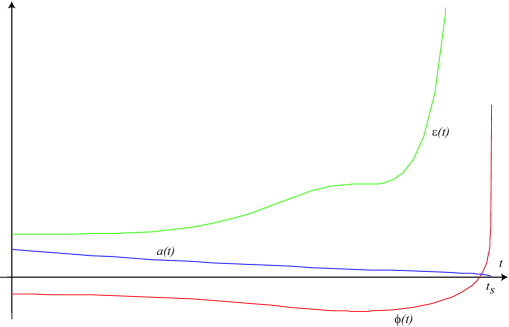
Figure 1. Behavior of the function $\phi(t),\epsilon(t)$, and $a(t)$ with potential given by $V(\phi)=1-\phi^{2}+\phi^{4}$. The initial conditions are $\phi_{0}=-0.6,\,\dot{\phi}_{0}=0,\,a_{0}=1$. The time of collapse $t_{s}$ approximately equals $t_{s}=2.1$.

For instance, for a quartic potential $V(\phi)=-\frac{1}{2}m^{2}\phi^{2}+\lambda^{2}\phi^{4}$, with $\lambda,m\neq 0$, the function $u(\phi)$ goes as $\tfrac{2}{\sqrt{3}\phi}$ for $\phi\to+\infty$, and all conditions listed above hold. The behavior for a particular example from this class of potential is given in Figure 1.

Example 3.10.

In the case of exponential potentials, the results hold for asymptotic behaviors with leading term at infinity of the form $V_{0}e^{2\sqrt{3}\lambda|\phi|}$ with $\lambda<1$. Consider for instance $V(\phi)=V_{0}\cosh(2\sqrt{3}\lambda\phi)$, where $V_{0},\lambda>0$: the quantity $u(\phi)$ goes like $\lambda$, and so (2.3) is verified if $\lambda<1$.

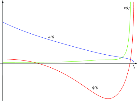
Figure 2. Same as Figure 1, but now the potential is given by $V(\phi)=\cosh(\sqrt{6}\phi)/100$. The initial conditions are $\phi_{0}=0.1,\,\dot{\phi}_{0}=0,\,a_{0}=1$. The time of collapse $t_{s}$ approximately equals $t_{s}=18.6$.

See a particular situation from this class represented in Figure 2.

Example 3.11.

Decaying exponential potentials can be considered as well. For instance for $V(\phi)=(1-e^{-\alpha\sqrt{\phi^{2}+\gamma^{2}}})^{2}$ the function $u(\phi)$ behaves like $e^{-\alpha|\phi|}$, so it goes to zero at $\pm\infty$.

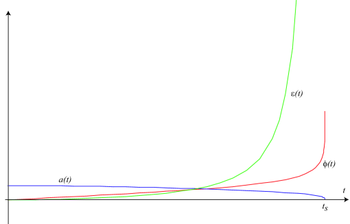
Figure 3. Same as Figure 1, where now $V(\phi)=2(1-e^{-\sqrt{x^{2}+1}})^{2}-\tfrac{1}{6}e^{-(x+4)^{2}}-\tfrac{1}{2}e^{-(x-4)^{2}}+1$. The initial conditions are $\phi_{0}=0,\,\dot{\phi}_{0}=\sqrt{-2V(0)},\,a_{0}=1$. The time of collapse $t_{s}$ approximately equals $t_{s}=1.8$.

Figure 3 represent a situation where some corrections terms have been added in order to obtain a potential with more than one critical points. Even choosing initial data such that $\epsilon_{0}=0$, the solution diverges in a finite amount of time, as showed in general in the second part of the proof of Theorem 3.7.

4. Gravitational collapse models

In what follows, we construct models of collapsing objects composed by homogeneous scalar fields. To achieve this goal we must match a collapsing solution (considered as the interior solution in matter) with an exterior spacetime. The natural choice for the exterior is the so–called generalized Vaidya solution

(4.1) $$\text{d}s_{\mathrm{ext}}^{2}=-\left(1-\frac{2M(U,Y)}{Y}\right)\,\mathrm{d}U^{2}-2\,\mathrm{d}Y\,\mathrm{d}U+Y^{2}\,\mathrm{d}\Omega^{2},$$

where $M$ is an arbitrary (positive) function (we refer to [27] for a detailed physical discussion of this spacetime, which is essentially the spacetime generated by a radiating object). The matching is performed along a hypersurface $\Sigma$ which, in terms of a spherical system of coordinates for the interior, has the simple form $r=r_{b}=const$. The Israel junction conditions at the matching hypersurface read as follows [9]:

(4.2) $$M(U(t),Y(t))=\frac{1}{2}r_{b}^{2}a(t)\dot{a}(t)^{2},$$

(4.3) $$\frac{\partial M}{\partial Y}(U(t),Y(t))=\frac{1}{2}r_{b}^{3}(\dot{a}(t)^{2}+2a(t)\ddot{a}(t)),$$

where the functions $(Y(t),U(t))$ satisfy

(4.4) $$Y(t)=r_{b}a(t),\qquad\frac{\text{d}U}{\text{d}t}(t)=\frac{1}{1+\dot{a}(t)r_{b}}.$$

The two equations (4.2)–(4.3) are equivalent to require that Misner–Sharp mass $M$ is continuous and $\tfrac{\partial M}{\partial U}=0$ on the junction hypersurface $\Sigma$ (using (4.2)–(4.4) together with (2.5a)–(2.6), it can be seen that in this way also the equation of motion for the scalar field remains smooth on the matching hypersurface).

The endstate of the collapse of these “homogeneous scalar field stars” is analyzed in the following theorem.

Theorem 4.1.

Except at most for a measure zero set of initial data, a scalar field ”star” collapses to a black hole.

Proof.

It is easy to check that the equation of the apparent horizon for the metric (2.1) is given by $r^{2}\dot{a}(t)^{2}=1$. If $\dot{a}$ is bounded, one can choose the junction surface $r=r_{b}$ sufficiently small such that $\dot{a}^{2}(t)<\tfrac{1}{r^{2}}$, $\forall(t,r)\in[0,t_{s}]\times[0,r_{b}]$, and so $\left(1-\tfrac{2M}{R}\right)$ is bounded away from zero near the singularity. As a consequence, one can find in the exterior portion of the spacetime (4.1), null radial geodesics which meet the singularity in the past, and therefore the singularity is naked; otherwise, if $\dot{a}^{2}$ is unbounded, the trapped region forms and the collapse ends into a black hole [9]. Now, we have proved in Lemma 3.5 the existence of $\rho_{\infty}=\lim_{\phi\to\infty}\rho(\phi)$ (which is also equal to $\lim_{t\to t_{s}^{-}}\rho(t)$), and that, actually, $\rho_{\infty}$ vanishes except for a zero–measured set of initial data. On the other hand, using (2.5b), we get

(4.5) $$\ddot{a}=-\frac{\dot{a}^{2}}{a}\left(\frac{2-\rho}{1+\rho}\right),$$

and therefore $\ddot{a}\leq-\tfrac{\dot{a}^{2}}{a}$ eventually holds in a left neighborhood of $t_{s}$, say $[t_{0},t_{s}[$, where $\dot{a}$ is decreasing. It follows that $\forall t\in]t_{0},t_{s}[$, $\dot{a}(t)\leq\dot{a}(t_{0})$, which is negative by hypotheses. Then

$$\dot{a}(t)-\dot{a}(t_{0})=\int_{t_{0}}^{t}\ddot{a}(\tau)\,\mathrm{d}\tau\leq-\int_{t_{0}}^{t}\frac{\dot{a}(\tau)^{2}}{a(\tau)}\,\mathrm{d}\tau\leq-\dot{a}(t_{0})\int_{t_{0}}^{t}\frac{\dot{a}(\tau)}{a(\tau)}\,\mathrm{d}\tau,$$

that diverges to $-\infty$. Then $\dot{a}(t)$ is unbounded. ∎

5. Naked singularities as examples of non-generic situations

As we have seen, the formation of naked singularities in the above discussed models is generically forbidden by theorem 4.1. Thus, the theorem does not exclude the existence of initial data which give rise to naked singularities for the given potential, it only assures that such data are non-generic. Actually, there are examples of such solutions containing naked singularities in the literature, and it is our aim here to show how they fit in this scenario.

To discuss this issue, it is convenient to reformulate the dynamics in the following form [9]. Since $a(t)$ is strictly decreasing in the collapsing case, we re-write equations (2.7), (2.9a) and (2.9b) using $a$ instead of $t$ as the independent variable. Setting

(5.1) $$\epsilon(a)=3\left(\frac{\psi(a)}{a}\right)^{2},$$

we get:

(5.2a) $$\dot{a} =-\psi(a),$$

(5.2b) $$\left(\frac{\text{d}\phi}{\text{d}a}\right)^{2} =\frac{1}{a^{2}}\left(1-a\frac{\psi^{\prime}(a)}{\psi(a)}\right),$$

(5.2c) $$V =\left(\frac{\psi(a)}{a}\right)^{2}\left(1+\frac{1}{2}a\frac{\psi^{\prime}(a)}{\psi(a)}\right),$$

In the above equations, $V(\phi)$ plays of course the same role of ”equation of state” as before. However, one can try to prescribe a part of the dynamics and then search if there is a choice of the potential and a set of data which assure that this dynamics is actually an admissible one for the system at hand (of course, in this way, only the ”on shell” value of the potential can be reconstructed). In particular, a somewhat natural approach can be that of prescribing the energy ($\epsilon(a)$ or equivalently $\Psi(a)$).

In [12], the case in which the energy density behaves like $a^{-\nu}$ with $\nu$ positive constant is considered. It is then shown that for $\nu<2$ the system forms a naked singularity, and the existence of an interval of values of $\nu$ is interpreted as a generic violation of cosmic censorship (that is anyway restored when loop quantum gravity modifications are taken into account, see [13]). However, due to the equation (5.2c) above, the on shell functional form of the potential for this example can be calculated to be $V(\phi)=V_{0}e^{2\sqrt{3}\lambda|\phi|}$ with $\lambda=\sqrt{\nu/6}$. This potential belongs to the class which has been treated in our previous example 3.10, and therefore we know that a generic choice of data must give rise to a blackhole (for this class the function $u(\phi)=V^{\prime}/(2\sqrt{3}V)$ behaves like a strictly positive constant $\lambda<1$). However, as we know from the proof of Lemma 3.5, a non generic situation can occur, when $\lim_{t\to t_{s}^{-}}u\sqrt{1+\rho}=1$ (where $\rho=2V/\dot{\phi}^{2}$); which means that $\lim_{\phi\to\infty}\rho(\phi)=\tfrac{1}{\lambda^{2}}-1=6/\nu-1$. Evaluating the function $\rho$ for the solution under study, we get exactly $\rho=6/\nu-1$. Therefore, the case discussed in [12, 13] is precisely the non-generic one. The constraint on the data which implies non-genericity comes, of course, from the fact that imposing a certain behavior on the function $\psi(a)$ selects a two-dimensional set in the space of the data, characterized by the algebraic constraint $\dot{\phi}(0)^{2}+2V(\phi(0))=3(\psi(a(0))/a(0))^{2}$.

To complete the analysis, we observe that, although the evolution of non generic data is not predicted by Theorem 3.7, we can easily obtain information also in this case. To this aim, observe that, since $\rho$ is finite, equation (3.13) can be used to prove singularity formation in a finite amount of comoving time with an argument similar to that used in the proof of Theorem 3.7. Moreover, the metric function $a(t)$ behaves asymptotically as $a_{0}(t_{s}-t)^{1/(3\lambda^{2})}$: then, if $\lambda<\sqrt{3}/3$, the function $\dot{a}(t)$ is bounded near the singularity, confirming naked singularity formation (this choice of $\lambda$ corresponds exactly to the choice of $\nu<2$ in [12]).

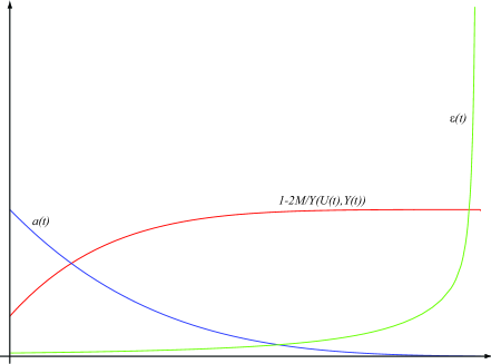
Figure 4. An example of naked singularity for $V(\phi)=0.01e^{\phi}$ for $\phi\geq 0$. The initial conditions are $\phi_{0}=0,\,\dot{\phi}_{0}=550^{-1/2},\,a_{0}=1$. The matching with external solution is performed at $r_{b}=100$. The time of collapse $t_{s}$ approximately equals $t_{s}=38.8$.

Figure 4 sketches an example of this kind: the initial data are chosen in the non generical way such that $\rho$ goes like a positive constant as $t\to t_{s}$. The singularity forms (i.e. $\epsilon(t)$ diverges in a finite time), but choosing $r_{b}$ not too large, the function $1-2M/Y$ on the junction hypersurface $r=r_{b}$ remains strictly positive along the evolution up to the singularity.

The above example suggests that hypotheses on the asymptotic behavior of the function $u(\phi)$ can be added, to obtain singularity formation also in the non generic case: indeed, if the potential $V(\phi)$ satisfies the condition

(5.3) $$\liminf_{\phi\to\pm\infty}|u(\phi)|>0,$$

i.e. $u(\phi)$ is definitely bounded away from zero, then $\rho$ is finite also in the non generic case, and equation (3.13) in the proof of Theorem 3.7 can be used to prove the formation of the singularity in a finite amount of time. To analyze the nature of this singularity observe that, if

(5.4) $$\liminf_{\phi\to\pm\infty}|u(\phi)|>\tfrac{\sqrt{3}}{3},$$

the argument in the proof of Theorem 4.1 applies, and therefore the collapse ends into a black hole. On the other side, if

(5.5) $$\limsup_{\phi\to\pm\infty}|u(\phi)|<\tfrac{\sqrt{3}}{3},$$

then $\ddot{a}$ is eventually positive, and this implies that $\dot{a}$ is bounded, so that the formation of the apparent horizon is forbidden. As a consequence, the collapse ends into a naked singularity.

6. Discussion and Conclusions

We have discussed here the qualitative behavior of the solutions of the Einstein field equations with homogeneous scalar fields sources in dependence of the choice of the self-interacting potential. It turns out that whenever a potential satisfies a certain set of general conditions singularity formation occurs for almost every choice of initial data. Matching these singular solutions with a Vaidya ”radiating star” exterior we obtained models of gravitational collapse which can be viewed as the scalar-field generalization of the Oppenheimer-Snyder collapse model, in which a dust homogeneous universe is matched with a Schwarzschild solution (the Schwarzschild solution can actually be seen as a special case of Vaidya).

The Oppenheimer-Snyder model, as is well known, describes the formation of a covered singularity, i.e. a blackhole; it is actually the first and simplest model of blackhole formation ever discovered. The same occurs here: indeed we show that homogeneous scalar field collapse generically forms a blackhole. The examples of naked singularities which were found in recent papers [9, 12], turn out to correspond to very special cases which, mathematically, are not generic. Therefore, our results here support the weak cosmic censorship conjecture, showing that naked singularities are not generic in homogeneous, self-interacting scalar field collapse.

Non-genericity was already well known for non self-interacting (i.e. $V(\phi)=0$) spherically symmetric scalar fields. Whether the results obtained here can actually be shown to hold also in the much more difficult case of both inhomogeneous and self-interacting scalar fields remains an open problem.

Appendix A Some properties of global solutions

We give here the proof that velocity and acceleration of solutions which extend indefinitely in the future must vanish asymptotically, if the values of the derivatives of the potential remain bounded on the corresponding flow.

Lemma A.1.

Let $\phi(t)$ a finite-energy solution of (2.9b), with $V\in\mathfrak{C}$. Then:

1) $\phi$ can be extended for all $t>0$,

2) if $V^{\prime}$ is bounded on the flow, then $\lim_{t\to+\infty}\dot{\phi}(t)=0$,

3) if also $V^{\prime\prime}$ is bounded on the flow then $\lim_{t\to+\infty}\ddot{\phi}(t)=0$.

Proof.

Since $\epsilon$ is bounded and $V$ is bounded from below, $\dot{\phi}$ is bounded as well, and thus $\phi$ can be extended for all $t$ (actually the existence of a lower bound for $V$ is the unique condition among A1)-A3) used here and below).

Using (2.10) we have

$$\int_{0}^{+\infty}\dot{\phi}(t)^{2}\,\mathrm{d}t=\int_{0}^{\infty}\frac{\dot{\epsilon}(t)}{2\sqrt{3}\sqrt{\epsilon(t)}}\,\mathrm{d}t<+\infty,$$

so there exists a sequence $t_{k}\to+\infty$ such that $\dot{\phi}(t_{k})\to 0$. By contradiction, suppose that $\exists\rho>0$, and a sequence $s_{k}\to t_{k}$ – that can be taken such that $s_{k}>t_{k}$ – with $|\dot{\phi}(s_{k})|>\rho$. Let $\bar{k}$ such that $|\dot{\phi}(t_{k})|<\tfrac{\rho}{2},\,\forall k\geq\bar{k}$, and let $\tau_{k},\sigma_{k}$ sequences such that $t_{k}\leq\tau_{k}<\sigma_{k}\leq s_{k}$, and

$$|\dot{\phi}(\tau_{k})|=\frac{\rho}{2},\qquad|\dot{\phi}(\sigma_{k})|=\rho,\qquad\frac{\rho}{2}\leq\dot{\phi}([\tau_{k},\sigma_{k}])|\leq\rho.$$

Note that $\epsilon$ bounded implies $\dot{\phi}$ bounded, while by assumption, $V^{\prime}(\phi(t))$ is bounded. Therefore by (2.8b), there exists $M>0$ such that

$$|\ddot{\phi}(t)|\leq M\qquad\forall t.$$

Therefore

$$\frac{\rho}{2}\leq|\dot{\phi}(\sigma_{k})-\dot{\phi}(\tau_{k})|\leq\int_{\tau_{k}}^{\sigma_{k}}|\ddot{\phi}(t)|\,\mathrm{d}t\leq M(\sigma_{k}-\tau_{k}),$$

that is $\sigma_{k}-\tau_{k}\geq\tfrac{\rho}{2M}$, and therefore

$$\int_{0}^{+\infty}\dot{\phi}(t)^{2}\,\mathrm{d}t\geq\sum_{k}\int_{\tau_{k}}^{\sigma_{k}}\dot{\phi}(t)^{2}\,\mathrm{d}t\geq\sum_{k}(\sigma_{k}-\tau_{k})\cdot\left(\frac{\rho}{2}\right)^{2}\geq\sum_{k}\frac{\rho^{3}}{8M},$$

that diverges. This is a contradiction, and therefore it must be $\lim_{t\to+\infty}\dot{\phi}(t)=0$.

To prove that the acceleration also vanish, let us first observe that $\exists t_{k}\to+\infty$ such that $V^{\prime}(\phi(t_{k}))\to 0$ – otherwise, there would exists $\kappa>0$ such that $|V^{\prime}(\phi(t))|\geq\kappa$ definitely, which would imply, in view of (2.8b), that $|\ddot{\phi}(t)|\geq\kappa/2$, that is absurd since $\lim_{t\to+\infty}\dot{\phi}(t)=0$.

Then, let us suppose by contradiction the existence of a constant $\rho>0$, and a sequence $s_{k}\to+\infty$ such that $t_{k}<s_{k}$ and $|V^{\prime}(\phi(s_{k}))|\geq\rho$. Therefore, one can choose $\sigma_{k},\tau_{k}$ sequences such that $t_{k}\leq\tau_{k}<\sigma_{k}\leq s_{k}$, and

$$|V^{\prime}(\phi(\tau_{k}))|=\frac{\rho}{2},\qquad|V^{\prime}(\phi(\sigma_{k}))|=\rho,\qquad\frac{\rho}{2}\leq|V^{\prime}(\phi(t))|\leq\rho,\,\forall t\in[\tau_{k},\sigma_{k}].$$

Then, since by assumption $V^{\prime\prime}(\phi(t))$ is bounded, there exists a constant $L>0$ such that

$$\frac{\rho}{2}=|V^{\prime}(\phi(\sigma_{k}))-V^{\prime}(\phi(\tau_{k}))|\leq\int_{\tau_{k}}^{\sigma_{k}}|V^{\prime\prime}(\phi(t))|\,|\dot{\phi}(t)|\,\text{d}t\leq L(\sigma_{k}-\tau_{k}).$$

But for sufficiently large $k$ let us observe that (2.8b) implies $|\ddot{\phi}(t)|\geq\rho/4$, $\forall t\in[\tau_{k},\sigma_{k}]$, and therefore $|\dot{\phi}(\sigma_{k})-\dot{\phi}(\tau_{k})|=|\int_{\tau_{k}}^{\sigma_{k}}\ddot{\phi}(t)\text{d}t|\geq\frac{\rho^{2}}{8L}$ that is a contradiction since $\dot{\phi}\to 0$. Thus $\lim_{t\to+\infty}V^{\prime}(\phi(t))=0$ vanishes, and equation (2.8b) implies that also $\ddot{\phi}$ vanishes in the same limit.

∎

Appendix B Local existence/uniqueness of solutions with initial zero–energy

Lemma B.1.

Let $\phi_{0},\,v_{0}$ such that $v_{0}^{2}+2V(\phi_{0})=0$. Then, there exists $t_{*}>0$ such that the Cauchy problem

(B.1) $$\begin{cases}&\ddot{\phi}(t)=-V^{\prime}(\phi(t))+\sqrt{3(\dot{\phi}(t)^{2}+2V(\phi(t)))}\,\dot{\phi}(t),\\ &\phi(0)=\phi_{0},\\ &\dot{\phi}_{0}=v_{0},\end{cases}$$

has a unique solution $\phi(t)$ defined in $[0,t_{*}]$ with the property

(B.2) $$\epsilon(t)=3\left(\int_{0}^{t}\dot{\phi}(s)^{2}\,\text{d}s\right)^{2},\,\forall t\in]0,t_{*}].$$

Moreover if $(\phi_{0,m},v_{0,m})\rightarrow(\phi_{0},v_{0})$, $(v_{0,m})^{2}+2V(\phi_{0,m})=0$ and $\phi_{m}$ is the solution of (B.1) with initial data $(\phi_{0,m},v_{0,m})$ satisfying condition (B.2), it is $\phi_{m}\rightarrow\phi$ with respect to the $C^{2}$-norm in the interval $[0,t_{*}]$.

Proof.

Let us consider the ”penalized” problem

(B.3) $$\begin{cases}&\ddot{\phi}(t)=-V^{\prime}(\phi(t))+\sqrt{3(\dot{\phi}(t)^{2}+2V(\phi(t))+\frac{1}{n^{2}})}\,\dot{\phi}(t),\\ &\phi(0)=\phi_{0},\\ &\dot{\phi}_{0}=v_{0},\end{cases}$$

that has a unique local solution $\phi_{n}$. If $\phi_{n}$ is not defined $\forall t\geq 0$, let $\mathds{I}_{n}$ be the set

$$\mathds{I}_{n}=\{t\in\mathds{R}\,:\,|\phi_{n}(s)|\leq|\phi_{0}|+1,\,|\dot{\phi}_{n}(s)|\leq|v_{0}|+1,\,\forall s\geq t\}.$$

Of course, $\mathds{I}_{n}\neq\emptyset$ and, called $t_{n}=\sup\mathds{I}_{n}$, if $t_{n}$ is finite, then $|\dot{\phi}_{n}(t_{n})|=|v_{0}|+1$, or $|\phi_{n}(t_{n})|=|\phi_{0}|+1$. Now assume $|\phi_{n}(t_{n})|=|\phi_{0}|+1$. Then

$$1=|\phi_{n}(t_{n})-\phi_{0}|\leq\int_{0}^{t_{n}}|\dot{\phi}_{n}(s)|\,\text{d}s\leq(|v_{0}|+1)t_{n}.$$

Analogously if $|\dot{\phi}_{n}(t_{n})|=|v_{0}|+1$ we have

$$1=|\dot{\phi}_{n}(t_{n})-v_{0}|\leq\int_{0}^{t_{n}}|\ddot{\phi}_{n}(s)|\,\text{d}s.$$

Since $|\phi_{n}(t)|\leq|\phi_{0}|+1$ and $|\dot{\phi}_{n}(s)|\leq|v_{0}|+1$ for all $t\in[0,t_{n}]$, and $\phi_{n}$ solves (B.3), we see that there exists $C$ independent of $n$ such that $|\ddot{\phi}(t)|\leq C$ for all $t\in[0,t_{n}]$. Therefore in this second case we obtain $1\leq Ct_{n}$.

Then $t_{*}:=\inf_{n}t_{n}>0$ (we set $t_{*}=1$ if $t_{n}=+\infty$ $\forall n$). Moreover $|\ddot{\phi}_{n}|$ is uniformly bounded in $[0,t_{*}]$, then up to subsequences, there exists a $\mathcal{C}^{1}$ function $\phi(t)$, solution of (B.1), such that $\phi_{n}\to\phi$ and $\dot{\phi}_{n}\to\dot{\phi}$ uniformly on $[0,t_{*}]$.

Now, consider $\epsilon_{n}(t):=\dot{\phi}_{n}(t)^{2}+2V(\phi_{n}(t))+\tfrac{1}{n^{2}}$. We have

(B.4) $$\dot{\epsilon}_{n}(t)=2\sqrt{3}\sqrt{\epsilon_{n}(t)}\dot{\phi}_{n}(t)^{2}.$$

Then $\epsilon$ is not decreasing, while $\epsilon(0)=\frac{1}{n}$. Then is uniformly bounded away from zero and therefore by (B.4), dividing by $\sqrt{\epsilon_{n}}$ and integrating gives $\sqrt{\epsilon_{n}(t)}=\tfrac{1}{n^{2}}+\sqrt{3}\int_{0}^{t}\dot{\phi}_{n}(s)^{2}\,\text{d}s$. Therefore passing to the limit in $n$ we obtain $\epsilon(t)=\dot{\phi}(t)^{2}+2V(\phi(t))=3\left(\int_{0}^{t}\dot{\phi}(s)^{2}\,\text{d}s\right)^{2}$ for all $t\in[0,t_{*}]$ obtaining the proof of the existence of a solution.

The uniqueness of such a solution can be obtained by a contradiction argument. Assuming $\phi$ and $\psi$ solutions, and called $\theta=\phi-\psi$, one can obtain, using (B.1), the estimate

$$|\dot{\theta}(t)|\leq K_{1}\int_{0}^{t}|\theta(s)|\,\text{d}s+K_{2}\int_{0}^{t}|\dot{\theta}(s)|\,\text{d}s,$$

for suitable constants $K_{1},K_{2}$. Setting $\rho(t)=|\theta(t)|+|\dot{\theta}(t)|$, and observing that $\rho(0)=0$, it is not hard to get the estimate $\rho(t)\leq(K_{1}+K_{2}+1)\int_{0}^{t}\rho(s)\,\text{d}s$, and then $\rho\equiv 0$ from Gronwall’s inequality.

Finally using Gronwall’s Lemma as above we obtain also the continuity with respect to the initial data. ∎

Remark B.2.

Reversing time direction in the above discussed problem (B.1) yields a results of genericity for expanding solutions such that the energy $\epsilon(t)$ vanishes at some finite time $T$.

References

- [1] M.S. Berger, Nonlinearity and Functional Analysis, Academic Press: New York, 1977.
- [2] M. Bojowald, M. Kagan Class.Quant.Grav. 23 (2006) 4983-4990
- [3] D. Christodoulou, Ann. Math. 140 607 (1994).
- [4] D. Christodoulou, Ann. Math. 149 183 (1999).
- [5] V. Faraoni, M.N. Jensen, S.A. Theuerkauf Class.Quant.Grav. 23 (2006) 4215-4230
- [6] Foster, S. arXiv:gr-qc/9806113 Scalar Field Cosmological Models With Hard Potential Walls
- [7] Foster, S. Class.Quant.Grav. 15 (1998) 3485-3504
- [8] R. Giambò, F. Giannoni, G. Magli, P. Piccione, Comm. Math. Phys. 235(3) 545-563 (2003)
- [9] R. Giambò, Class. Quantum Grav. 22 (2005) 1-11
- [10] R. Giambò, F. Giannoni, G. Magli, J. Math. Phys., 47 112505 (2006)
- [11] R. Giambò, F. Giannoni, G. Magli, arXiv:0802.0157 [gr-qc]
- [12] P. S. Joshi, Gravitational collapse and spacetime singularities, Cambridge University Press, 2007
- [13] R. Goswami, P. S. Joshi, P. Singh, Phys. Rev. Lett. 96, 031302 (2006)
- [14] Hertog,T., Horowitz, G.T., and Maeda K., Phys. Rev. Lett. 92, 131101 (2004)
- [15] Hertog,T., Horowitz, G.T., and Maeda K., arXiv:gr-qc/0405050v2
- [16] Hertog, T. Phys.Rev. D74 (2006) 084008
- [17] P. S. Joshi, Modern Phys. Lett. A 17 1067–1079 (2002)
- [18] J. Miritzis, J. Math. Phys. 44 (2003) 3900-3910
- [19] J. Miritzis, J. Math. Phys. 46 (2005) 082502
- [20] C. Rubano, J. D. Barrow, Phys.Rev. D64 (2001) 127301
- [21] C. Rubano, P. Scudellaro Gen.Rel.Grav. 34 (2002) 307-328
- [22] A.D. Rendall Class.Quant.Grav. 21 (2004) 2445-2454
- [23] A.D. Rendall Class.Quant.Grav. 24 (2007) 667-678
- [24] A.D. Rendall, Gen.Rel.Grav. 34 (2002) 1277-1294
- [25] Russo, J. G. Phys. Lett. B 600 p- 185-190 (2004)
- [26] Toporensky A.V., Internat. J. Modern Phys. D, 1999, V.8, 739?750.
- [27] A. Wang and Y. Wu, 1999 Gen. Rel. Grav. 31 107