A note on the violation of the Einstein relation in a driven moderately dense granular gas

Abstract

The Einstein relation for a driven moderately dense granular gas in $d$-dimensions is analyzed in the context of the Enskog kinetic equation. The Enskog equation neglects velocity correlations but retains spatial correlations arising from volume exclusion effects. As expected, there is a breakdown of the Einstein relation $\epsilon=D/(T_{0}\mu)\neq 1$ relating diffusion $D$ and mobility $\mu$, $T_{0}$ being the temperature of the impurity. The kinetic theory results also show that the violation of the Einstein relation is only due to the strong non-Maxwellian behavior of the reference state of the impurity particles. The deviation of $\epsilon$ from unity becomes more significant as the solid volume fraction and the inelasticity increase, especially when the system is driven by the action of a Gaussian thermostat. This conclusion qualitatively agrees with some recent simulations of dense gases [Puglisi et al., 2007 J. Stat. Mech. P08016], although the deviations observed in computer simulations are more important than those obtained here from the Enskog kinetic theory. Possible reasons for the quantitative discrepancies between theory and simulations are discussed.

I Introduction

The generalization of the fluctuation-response relation to non-equilibrium systems has received a considerable attention in the past few years. In this context, granular matter can be considered as a good example of a system that inherently is in a non-equilibrium state. Granular systems are constituted by macroscopic grains that collide inelastically so that the total energy decreases with time. On the other hand, a non-equilibrium steady state (NESS) is reached when the system is heated by the action of an external driving force (thermostat) that does work to compensate for the collisional loss of energy. In these conditions, some attempts to formulate a fluctuation-response theorem based on the introduction of an effective temperature have been carried out PBL02 ; SD04 ; SBL06 ; BSL08 . However, a complete analysis of the validity of the theorem requires the knowledge of the full dependence of the response and correlation functions on frequency $\omega$ L89 . Given that this dependence is quite difficult to evaluate in general, the corresponding limit $\omega\to 0$ is usually considered. In this limit, the classical relation between the coefficients of diffusion $D$ (autocorrelation function) and mobility $\mu$ (linear response) is known as the Einstein relation.

The Einstein relation for heated granular fluids has been widely analyzed recently. First, some computer simulation results for dilute systems BLP04 have shown the validity of the Einstein relation ($\epsilon=D/T_{0}\mu=1$) in NESS when the temperature of the bath $T$ is replaced by the temperature of the impurity $T_{0}$. This has an interesting consequence in the case of mixtures (where the different species have different temperatures GD99 ; nonequip ; exp ) since a linear response experiment on a massive intruder or tracer particle to obtain a temperature measurement yields the temperature of the intruder and not the temperature of the surrounding gas. On the other hand, from an analytical point of view, kinetic theory calculations based on the Boltzmann equation have shown the violation of the Einstein relation ($\epsilon\neq 1$) in the free cooling case DG01 as well as for driven granular gases G04 . These deviations are in general very small in the driven case (less than $1\%$ when the system is driven by a stochastic thermostat) and are related to non-Gaussian properties of the distribution function of the impurities. This is the reason why such deviations cannot be detected in computer simulations of very dilute gases.

However, a recent computer simulation study of Puglisi et al. PBV07 at high densities has provided evidence that the origin of the violation of the Einstein formula is mainly due to spatial and velocity correlations between the particles that are about to collide rather than the deviation from the Maxwell-Boltzmann statistics. These correlations increase as excluded volume and energy dissipation occurring in collisions are increased. The simulation results obtained by Puglisi et al. PBV07 motivate the present paper and, as in the case of a dilute gas G04 , kinetic theory tools will be used to analyze the effect of density on the possible violation of the Einstein relation. For a moderately dense gas, the Enskog kinetic equation for inelastic hard spheres BDS97 can be considered as an accurate and practical generalization of the Boltzmann equation. As in the case of elastic collisions, the Enskog equation takes into account spatial correlations through the pair correlation function but neglects velocity correlations (molecular chaos assumption) F72 . Although the latter assumption has been shown to fail for inelastic collisions as the density increases ML98 ; SM01 ; PTNE02 , there is substantial evidence in the literature for the validity of the Enskog theory for densities outside the Boltzmann limit (moderate densities) and values of dissipation beyond the quasielastic limit. This evidence is supported by the good agreement found at the level of macroscopic properties (such as transport coefficients) between the Enskog theory GD99b ; L05 ; GDH07 and simulation L01 ; LBD02 ; DHGD02 ; MGAL06 ; LLC07 and experimental YHCMW02 ; HYCMW04 results. In this context, one can conclude that the Enskog equation provides a unique basis for the description of dynamics across a wide range of densities, length scales, and degrees of dissipation. No other theory with such generality exists.

II Description of the problem

Let us consider a granular gas composed by smooth inelastic disks ($d=2$) or spheres ($d=3$) of mass $m$, diameter $\sigma$, and interparticle coefficient of restitution $\alpha$ in a homogeneous state. At moderate densities, we assume that the velocity distribution function $f({\bf v})$ obeys the Enskog kinetic equation BDS97 . Due to dissipation in collisions, the gas cools down unless a mechanism of energy input is externally introduced to compensate for collisional cooling. In experiments the energy is typically injected through the boundaries yielding an inhomogeneous steady state. To avoid the complication of strong temperature heterogeneities, it is usual to consider the action of homogeneous external (driving) forces acting locally on each particle. These forces are called thermostats and depend on the state of the system. In this situation, the steady-state Enskog equation reads

$${\cal F}f({\bf v})=\chi J[{\bf v}|f,f],$$ (1)

where $J[{\bf v}|f,f]$ is the inelastic Boltzmann collision operator, $\chi$ denotes the equilibrium configurational pair correlation function evaluated at contact, and ${\cal F}$ is an operator representing the effect of the external force. Two types of external forces (thermostats) are usually considered: (a) a deterministic force proportional to the particle velocity (Gaussian thermostat), and (b) a white noise external force (stochastic thermostat). The use of these kinds of thermostats has attracted the attention of granular community in the past years to study different problems. In the case of the Gaussian thermostat, ${\cal F}$ has the form EM90 ; H91 ; MS00

$${\cal F}f({\bf v})=\frac{1}{2}\zeta\frac{\partial}{\partial{\bf v}}\cdot\left[{\bf v}f({\bf v})\right],$$ (2)

where $\zeta$ is the cooling rate due to collisions. In the case of the stochastic thermostat, the operator ${\cal F}$ has the Fokker-Planck form NE98

$${\cal F}f({\bf v})=-\frac{1}{2}\frac{T}{m}\zeta\left(\frac{\partial}{\partial{\bf v}}\right)^{2}f({\bf v}).$$ (3)

The exact solution to the Enskog equation (1) is not known, although a good approximation for $f$ in the region of thermal velocities can be obtained from an expansion in Sonine polynomials. For practical purposes, one selects a finite number of terms in the expansion. In the leading order $f({\bf v})$ is given by

$$f({\bf v})\to n\pi^{-d/2}v_{\text{th}}^{-d}e^{-v^{*2}}\left[1+\frac{c}{4}\left(v^{*4}-(d+2)v^{*2}+\frac{d(d+2)}{4}\right)\right],$$ (4)

where ${\bf v}^{*}={\bf v}/v_{\text{th}}$, $v_{\text{th}}=\sqrt{2T/m}$ being the thermal velocity. Moreover, $c$ is the fourth cumulant of the velocity distribution function $f$ defined as

$$c=\frac{8}{d(d+2)}\left(\frac{m^{2}}{4nT^{2}}\int\;d{\bf v}\;v^{4}f-\frac{d(d+2)}{4}\right).$$ (5)

In the approximation (4), cumulants of higher order have been neglected. Inserting Eq. (4) into the Enskog equation and neglecting nonlinear terms in $c$, one gets the following expression for the cooling rate $\zeta$ NE98

$$\zeta=\frac{\sqrt{2}\pi^{(d-1)/2}}{d\Gamma\left(\frac{d}{2}\right)}\chi n\sigma^{d-1}v_{\text{th}}(1-\alpha^{2})\left(1+\frac{3}{32}c\right).$$ (6)

The value of $c$ depends on the thermostat used. In the case of the Gaussian thermostat, $c$ is approximately given by NE98

$$c(\alpha)=\frac{32(1-\alpha)(1-2\alpha^{2})}{9+24d-(41-d)\alpha+30\alpha^{2}(1-\alpha)},$$ (7)

while

$$c(\alpha)=\frac{32(1-\alpha)(1-2\alpha^{2})}{73+56d-3(35+8d)\alpha+30\alpha^{2}(1-\alpha)}$$ (8)

for the stochastic thermostat. It is interesting to remark that in the homogeneous problem the results obtained with the Gaussian thermostat are completely equivalent to those derived in the free cooling case when one scales the particle velocity with respect to the thermal velocity $v_{\text{th}}$ MS00 . In addition, although the expressions (6)–(8) have been derived by neglecting nonlinear terms in the coefficient $c$, the estimates (7) and (8) present quite a good agreement with Monte Carlo simulations of the Boltzmann equation MS00 ; BMC96 for moderate values of dissipation (say for instance, $\alpha\gtrsim 0.5$). However, more recent results BP06 ; NBSG07 for the homogeneous (undriven) cooling state have shown that for very large inelasticity ($\alpha\lesssim 0.5$), the higher-order cumulants may not be neglected since they can be of the same order of magnitude as $c$. The breakdown of the Sonine polynomial expansion is caused by the increasing impact of the overpopulated high-energy tail of the velocity distribution $f$ PBF06 .

We assume now that a few impurities or tracer particles of mass $m_{0}$ and diameter $\sigma_{0}$ are added to the system. Given that their concentration is very small, the state of the gas is not affected by the presence of impurities. As a consequence, the velocity distribution function $f$ of the gas still verifies the (homogeneous) Enskog equation (1). Moreover, one can also neglect collisions among impurities themselves versus the impurity-gas collisions, which are characterized by the coefficient of restitution $\alpha_{0}$. Diffusion of impurities is generated by a weak concentration gradient $\nabla n_{0}$ and/or a weak external field ${\bf E}$ (e.g. gravity or an electric field) acting only on the impurity particles. Under these conditions, the velocity distribution function $f_{0}({\bf r},{\bf v},t)$ of impurities verifies the Enskog-Lorentz equation

$$\partial_{t}f_{0}+{\bf v}\cdot\nabla f_{0}+\frac{{\bf E}}{m_{0}}\cdot\frac{\partial}{\partial{\bf v}}f_{0}+{\cal F}f_{0}=\chi_{0}J[{\bf v}|f_{0},f],$$ (9)

where $J\left[f_{0},f\right]$ is the (inelastic) Boltzmann-Lorentz collision operator and $\chi_{0}$ represents the equilibrium pair correlation function for impurity-fluid pairs at contact. Given that the gas is in a homogeneous state, it follows that $\chi_{0}$ is uniform. At a kinetic level, an interesting quantity is the partial temperature of impurities $T_{0}$. It is defined as

$$\frac{d}{2}n_{0}T_{0}=\int\,d{\bf v}\,\frac{m_{0}}{2}v^{2}f_{0}({\bf v}),$$ (10)

where $n_{0}$ is the number density of impurities. The corresponding cooling rate $\zeta_{0}$ associated with the partial temperature $T_{0}$ of impurities is defined as

$$\zeta_{0}=-\frac{\chi_{0}}{dn_{0}T_{0}}\int d{\bf v}m_{0}v^{2}J[{\bf v}|f_{0},f].$$ (11)

Figure 1: Plot of the temperature ratio $T_{0}/T$ versus the coefficient of restitution $\alpha=\alpha_{0}$ for $d=3$ in the case $m_{0}/m=\sigma_{0}/\sigma=0.5$ for the Gaussian thermostat (a) and the stochastic thermostat (b). The solid lines correspond to a dilute gas ($\phi=0$) while the dashed lines refer to a moderately dense gas ($\phi=0.2$).

Figure 2: Plot of the coefficient $c_{0}$ versus the coefficient of restitution $\alpha=\alpha_{0}$ for $d=3$ in the case $m_{0}/m=\sigma_{0}/\sigma=0.5$ for the Gaussian thermostat (a) and the stochastic thermostat (b). The solid lines correspond to a dilute gas ($\phi=0$) while the dashed lines refer to a moderately dense gas ($\phi=0.2$).

In the absence of diffusion (homogeneous steady state), Eq. (9) becomes

$${\cal F}f_{0}=\chi_{0}J[{\bf v}|f_{0},f].$$ (12)

This equation has been widely analyzed by using both types of thermostats DHGD02 ; G04 for hard spheres ($d=3$). The results show that the temperatures of the gas ($T$) and impurities ($T_{0}$) are clearly different and so the energy equipartition is broken down. In general, the temperature ratio $\gamma\equiv T_{0}/T$ presents a complex dependence on the parameters of the problem. The condition for determining the temperature ratio $\gamma$ is different for each type of thermostat. In the case of the Gaussian thermostat, the temperature ratio is obtained by equating the cooling rates GM04 ; GD99

$$\zeta=\zeta_{0},$$ (13)

while for the stochastic thermostat $\gamma$ is obtained from the condition DHGD02

$$\frac{\zeta T}{m}=\frac{\zeta_{0}T_{0}}{m_{0}}.$$ (14)

Requirements (13) and (14) lead to a different dependence of the temperature ratio $T_{0}/T$ on the control parameters, namely, the mass ratio $m_{0}/m$, the size ratio $\sigma_{0}/\sigma$, the coefficients of restitution $\alpha$ and $\alpha_{0}$, and the solid volume fraction

$$\phi\equiv\frac{\pi^{d/2}}{2^{d-1}d\Gamma\left(\frac{d}{2}\right)}n\sigma^{d}.$$ (15)

Apart from the temperature ratio, an interesting quantity is the fourth cumulant $c_{0}$. It is defined as

$$c_{0}=\frac{8}{d(d+2)}\left(\frac{m_{0}^{2}}{4n_{0}T_{0}^{2}}\int\;d{\bf v}\;v^{4}f_{0}-\frac{d(d+2)}{4}\right).$$ (16)

As in the case of the coefficient $c$, the cumulant $c_{0}$ measures the deviation of $f_{0}$ from its Maxwellian form

$$f_{0,M}({\bf v})=n_{0}\left(\frac{m_{0}}{2T_{0}}\right)^{d/2}\exp\left(-\frac{m_{0}v^{2}}{2T_{0}}\right).$$ (17)

In order to determine the coefficients $\zeta_{0}$ and $c_{0}$ one has to expand the velocity distribution function $f_{0}$ in terms of the orthogonal Sonine polynomials. As in the case of the granular gas distribution $f$, a good estimate of $\zeta_{0}$ and $c_{0}$ can be obtained from the leading Sonine approach to $f_{0}$:

$$f_{0}({\bf v})\to n_{0}\pi^{-d/2}v_{\text{th}}^{-d}\theta^{d/2}e^{-\theta v^{*2}}\left[1+\frac{c_{0}}{4}\left(\theta^{2}v^{*4}-(d+2)\theta v^{*2}+\frac{d(d+2)}{4}\right)\right],$$ (18)

where $\theta=m_{0}T/mT_{0}$ is the mean square velocity of the gas particles relative to that of impurities. Expressions for $\zeta_{0}$ and $c_{0}$ have been derived in Appendix A for an arbitrary number of dimensions $d$ by considering only linear terms in $c$ and $c_{0}$. These expressions extend previous results derived in Ref. G04 for hard spheres. Once $\zeta_{0}$ and $c_{0}$ are known, the temperature ratio can be obtained from the constraints (13) and (14) for the Gaussian and stochastic thermostats, respectively. To get this explicit dependence, the form of the pair correlation functions $\chi$ and $\chi_{0}$ in terms of the size ratio $\sigma_{0}/\sigma$ and the solid volume fraction $\phi$ must be given. For a three-dimensional gas ($d=3$), a good approximation for these functions is GH72

$$\chi=\frac{1-\frac{1}{2}\phi}{(1-\phi)^{3}},$$ (19)

$$\chi_{0}=\frac{1}{1-\phi}+\frac{3}{2}\frac{\sigma_{0}}{\overline{\sigma}}\frac{\phi}{(1-\phi)^{2}}+\frac{1}{2}\left(\frac{\sigma_{0}}{\overline{\sigma}}\right)^{2}\frac{\phi^{2}}{(1-\phi)^{3}},$$ (20)

where $\overline{\sigma}=(\sigma+\sigma_{0})/2$. For a two-dimensional gas ($d=2$), $\chi$ and $\chi_{0}$ are approximately given by JM87

$$\chi=\frac{1-\frac{7}{16}\phi}{(1-\phi)^{2}},$$ (21)

$$\chi_{0}=\frac{1}{1-\phi}+\frac{9}{16}\frac{\sigma_{0}}{\overline{\sigma}}\frac{\phi}{(1-\phi)^{2}}.$$ (22)

Obviously, $\chi=\chi_{0}$ if $\sigma=\sigma_{0}$. Thus the temperature ratio and the kurtosis $c_{0}$ become independent of density for equal–size particles. The dependence of $T_{0}/T$ on the (common) coefficient of restitution $\alpha=\alpha_{0}$ is illustrated in Fig. 1 for $d=3$ in the case $m_{0}/m=\sigma_{0}/\sigma=0.5$ and for two values of the solid volume fraction $\phi$. We consider the two types of thermostats discussed before. There is an evident breakdown of the energy equipartition in both thermostats, especially in the case of the stochastic driving force (3). However, the influence of density is more significant for the Gaussian thermostat than for the stochastic one. The dependence of $c_{0}$ on $\alpha_{0}$ is plotted in Fig. 2 for the same cases as considered in Fig. 1. It is apparent that for both thermostats the value of $c_{0}$ is quite small for not too inelastic systems. This means that in this range of values of $\alpha_{0}$ the distribution $f_{0}$ of the homogeneous state is quite close to a Maxwellian at the temperature of the impurity particle $T_{0}$. However, the magnitude of $c_{0}$ increases significantly as the dissipation increases, especially in the case of the Gaussian thermostat. This is a signal of the strong non-Maxwellian behavior of the reference homogeneous state of impurities for quite extreme values of inelasticity. As a consequence, cumulants of higher order than the fourth cumulant $c_{0}$ should be considered to assess the deviation of $f_{0}$ from its Maxwellian form $f_{0,M}$ for very small values of $\alpha$ and $\alpha_{0}$. Finally, with respect to the influence of density, we observe that it is more relevant for the Gaussian thermostat than for the stochastic thermostat, being practically negligible in the latter case.

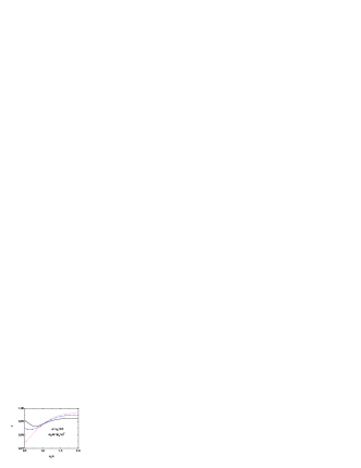
Figure 3: (Color online) Plot of the Einstein ratio $\epsilon=D/T_{0}\mu$ versus the size ratio $\sigma_{0}/\sigma$ in the case of the Gaussian thermostat for $d=3$ and $\alpha=\alpha_{0}=0.5$ when the impurities have the same mass density as the gas particles. Three different values of the solid volume fraction are considered: $\phi=0$ (solid line), $\phi=0.2$ (dashed line), and $\phi=0.4$ (dotted line).

III The Einstein relation

The Einstein ratio $\epsilon$ is defined as

$$\epsilon=\frac{D}{T_{0}\mu},$$ (23)

where $D$ and $\mu$ are the diffusion and mobility coefficients, respectively. If the Einstein relation would hold, one would have $\epsilon=1$. I want here to analyze the influence of density on $\epsilon$. The transport coefficients $D$ and $\mu$ can be determined by solving the (inelastic) Enskog-Lorentz equation (9) by means of the Chapman-Enskog method CC70 . In the first order of the expansion, the current of impurities ${\bf j}_{0}$ has the form G04

$${\bf j}_{0}=-D\nabla\ln n_{0}+\mu{\bf E}.$$ (24)

Given that $\chi$ and $\chi_{0}$ are uniform in this problem, it is evident that, when properly scaled, the previous solution obtained in Ref. G04 for a dilute gas can be directly translated to the Enskog equation by making the changes $J[f,f]\to\chi J[f,f]$ and $J[f_{0},f]\to\chi_{0}J[f_{0},f]$. Technical details on the calculation of $D$ and $\mu$ by means of the Chapman-Enskog expansion CC70 up to the second Sonine approximation can be found in Ref. G04 for inelastic hard spheres ($d=3$). The extension to an arbitrary number of dimensions is straighforward. Taking into account these results, the dependence of the Einstein ratio $\epsilon$ on the parameter space of the problem can be obtained. In the case of the Gaussian thermostat, the result is

$$\epsilon=1-\frac{c_{0}}{2}\frac{\nu_{2}}{\nu_{4}-\frac{3}{2}\zeta},$$ (25)

where the collision frequencies $\nu_{2}$ and $\nu_{4}$ are explicitly given in Appendix A for an arbitrary number of dimensions $d$. The result for the case of the stochastic thermostat is

$$\epsilon=1-\frac{c_{0}}{2}\frac{\nu_{2}}{\nu_{4}}.$$ (26)

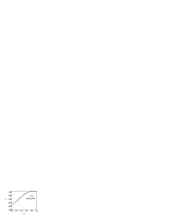
Figure 4: (Color online) Plot of the Einstein ratio $\epsilon=D/T_{0}\mu$ versus the coefficient of restitution $\alpha=\alpha_{0}$ in the case of the Gaussian thermostat for $d=2$, $m_{0}/m=\sigma_{0}/\sigma=0.5$ and three different values of the solid volume fraction: $\phi=0$ (solid line), $\phi=0.2$ (dashed line), and $\phi=0.4$ (dotted line).

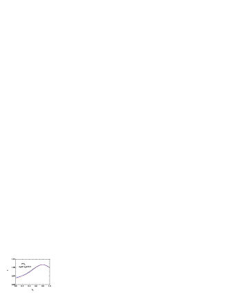
Figure 5: (Color online) Plot of the Einstein ratio $\epsilon=D/T_{0}\mu$ versus the coefficient of restitution $\alpha=\alpha_{0}$ in the case of the stochastic thermostat for $d=2$, $m_{0}/m=\sigma_{0}/\sigma=0.5$ and three different values of the solid volume fraction: $\phi=0$ (solid line), $\phi=0.2$ (dashed line), and $\phi=0.4$ (dotted line).

Figure 6: Plot of the ratio $\epsilon(\phi)/\epsilon(0)$ versus the solid volume fraction $\phi$ for $\alpha=\alpha_{0}=0.5$, $m_{0}/m=2$ and $\sigma_{0}/\sigma=0.25$ in the case of the Gaussian thermostat for spheres ($d=3$) and disks ($d=2$).

It is clear that $\epsilon$ becomes independent of the density $\phi$ when $\sigma=\sigma_{0}$. As in the case of dilute gases G04 , Eqs. (25) and (26) show that the violation of the Einstein relation in a heated moderately dense granular gas is basically due to the departures of $f_{0}$ from its Maxwellian form $f_{0,M}$. At this level of approximation (second Sonine approximation to the coefficients $D$ and $\mu$), the deviation of $f_{0}$ from $f_{0,M}$ is only accounted for by the fourth cumulant $c_{0}$. However, the coefficient $c_{0}$ depends on the solid volume fraction $\phi$ through its dependence on the temperature ratio $T_{0}/T$. To assess the influence of density on the Einstein ratio $\epsilon$, Fig. 3 shows a plot of $\epsilon$ versus the size ratio $\sigma_{0}/\sigma$ in the case of the Gaussian thermostat for $d=3$ and $\alpha=\alpha_{0}=0.5$ when the impurities have the same mass density as the gas particles [namely, $m_{0}/m=(\sigma_{0}/\sigma)^{3}$]. Three different values of the solid volume fraction $\phi$ have been considered: $\phi=0$ (dilute gas), $\phi=0.2$ (moderate dense gas), and $\phi=0.4$ (quite dense gas). The corresponding plot for the stochastic thermostat has not been included since the deviation of $\epsilon$ from 1 is less than $1\%$ for all the cases analyzed. It is apparent that the degree of violation of the Einstein relation is more important when the impurities are lighter and/or smaller than the gas particles, especially for high densities. To confirm this trend, the Einstein ratio has been plotted in Figs. 4 and 5 as a function of the (common) coefficient of restitution $\alpha=\alpha_{0}$ for $d=2$, $m_{0}/m=\sigma_{0}/\sigma=0.5$, and for the same values of $\phi$ as considered before. Figure 4 shows the results obtained by using the Gaussian thermostat and Fig. 5 refers to the results obtained for the stochastic thermostat. While $\epsilon$ is close to 1 in the case of the stochastic thermostat for all the densities considered, significant deviations form unity are observed for the Gaussian thermostat. In this latter case, it is apparent that the degree of violation of the Einstein formula increases with the volume fraction and the inelasticity.

This latter conclusion qualitatively agrees with the results obtained by Puglisi et al. PBV07 from computer simulations since they observe a significant violation of the Einstein formula when excluded volume effects and dissipation are increased. However, at a quantitative level, the deviations observed by Puglisi et al. PBV07 are larger than those found here [see Fig. 3 of Ref. PBV07 ]. The quantitative disagreement between simulations PBV07 and the Enskog theory results (25) and (26) could be due to two different and independent reasons. First, as noted before in Section II, the expression of the fourth cumulant $c_{0}$ used here has been obtained by neglecting cumulants of higher order and considering only linear terms in $c$ and $c_{0}$. On the other hand, according to the previous results BP06 ; NBSG07 obtained in the free cooling case for a monocomponent gas, the value of $c_{0}$ could change significantly for very strong dissipation when cumulants of higher order were taken into account in the form of the homogeneous distribution. In this context, the estimate of $c_{0}$ obtained in this paper could be not reliable for this range of values of inelasticity and so, the quantitative deviations of $\epsilon$ from $1$ observed in Figs. 3 and 4 for the Gaussian thermostat when $\alpha_{0}\lesssim 0.5$ could be questionable. As a second reason of discrepancy between simulations and theory, one could argue that the velocity correlations (absent in the Enskog equation but present in computer simulations) play a more important role than spatial correlations (excluded volume effects) in the violation of the Einstein formula. In this case, one should correct the Enskog equation by incorporating recollision events (“ring” collisions) that take into account multiparticle collisions.

Finally, since the results derived in this paper holds for a $d$-dimensional system, it is interesting to investigate the influence of dimensionality on the violation of the Einstein relation. To illustrate this effect, Fig. 6 shows the dependence of the ratio $\epsilon(\phi)/\epsilon(0)$ on the solid volume fraction $\phi$ for $\alpha=\alpha_{0}=0.5$, $m_{0}/m=2$ and $\sigma_{0}/\sigma=0.25$ in the case of the Gaussian thermostat. I have considered the physical cases of hard spheres ($d=3$) and hard disks ($d=2$). Here, $\epsilon(0)$ corresponds to the value of the Einstein ratio for a dilute gas. Although the qualitative dependence of the ratio $\epsilon(\phi)/\epsilon(0)$ on $\phi$ is quite similar in both systems, we observe that the violation of the Einstein ratio is stronger for $d=3$ than for $d=2$ for moderate densities. However, this trend changes as density becomes larger.

IV Conclusions

In this paper I have analyzed the validity of the Einstein relation $\epsilon=D/T_{0}\mu=1$ for driven moderately $d$-dimensional dense granular gases in the framework of the Enskog equation. This work extends a previous study carried out by the author G04 in the case of a dilute gas ($\phi=0$) of inelastic hard spheres ($d=3$). To achieve a NESS, two types of thermostats (external forces) have been considered: (i) an “anti-drag” force proportional to the particle velocity (Gaussian force), and (b) a stochastic force, which give frequent kicks to each particle between collisions. The present work has been motivated by recent computer simulation results by Puglisi et al. PBV07 where the spatial and velocity correlations between the particles have shown to be the most important ingredient in a strong violation of the Einstein relation. It is shown that $\epsilon\neq 1$, especially in the case of the Gaussian thermostat when the impurity is lighter and/or smaller than particles of the gas. As in the case of a dilute gas G04 , the violation of the Einstein relation is connected to the strong non-Maxwellian behavior of the homogeneous velocity distribution function of impurities, which is mainly measured through its fourth cumulant $c_{0}$. The results also show that the deviation of the Einstein ratio from 1 is more important as both the density and dissipation increase, which is consistent with the observations made by Puglisi et al. PBV07 . However, at a quantitative level, the deviations of the Einstein formula obtained here from the Enskog equation are smaller than those found in computer simulations. As discussed before, this quantitative disagreement between theory and simulation could be due to (i) the possible lack of convergence of the Sonine polynomial expansion for the reference Gaussian driven state, and/or (ii) the influence of velocity correlations which are absent in the Enskog description (molecular chaos hypothesis). With respect to the first source of discrepancy, one perhaps should include cumulants of higher order as well as nonlinear terms in $c$ and $c_{0}$ to get an accurate estimate of the fourth cumulant $c_{0}$ for very small values of the coefficients of restitution $\alpha$ and $\alpha_{0}$. However, given that perhaps the absolute value of the higher order cumulants increases with inelasticity, the Sonine expansion could be not relevant in the sense that one would need an infinite number of Sonine coefficients to characterize the reference state. In this case, a possible alternative would be the use of the Direct Simulation Monte Carlo (DSMC) method B94 to numerically solve the Enskog equation in the homogenous driven problem. Regarding the influence of velocity correlations, the inclusion of this new ingredient in the Enskog collision operator makes analytic calculations intractable since higher-order correlations must be included in the evaluation of the collision integrals. This contrasts with the explicit results reported in this paper, where the transport coefficients $D$ and $\mu$ have been explicitly obtained in terms of the parameters of the system (masses, sizes and coefficients of restitution).

Finally, it must be noted that the theoretical results derived here have been obtained by considering the second Sonine approximation to the Chapman-Enskog solution. Exact results can be obtained if one considers the inelastic Maxwell model (IMM) for a dilute gas. This model has been widely used by several authors as a toy model to characterize the influence of the inelasticity of collisions of the physical properties of the granular fluids. The fact the the collision rate for the IMM is velocity independent allows one to exactly compute the transport coefficients of the system. In particular, the coefficients $D$ and $\mu$ have been evaluated GA05 from the Chapman-Enskog method for undriven systems. The extension of such calculations to driven systems is straightforward. Thus, in the case of the Gaussian thermostat, one gets

$$D=\frac{n_{0}T_{0}}{m_{0}}\left(\nu_{D}-\frac{1}{2}\zeta\right)^{-1},\quad\mu=\frac{n_{0}}{m_{0}}\left(\nu_{D}-\frac{1}{2}\zeta\right)^{-1},$$ (27)

while

$$D=\frac{n_{0}T_{0}}{m_{0}\nu_{D}},\quad\mu=\frac{n_{0}}{m_{0}\nu_{D}}$$ (28)

in the case of the stochastic thermostat. Here,

$$\nu_{D}=\frac{w_{0}}{d}\frac{m}{m+m_{0}}(1+\alpha_{0}),\quad\zeta=\frac{w}{2d}(1-\alpha^{2}),$$ (29)

where $w$ and $w_{0}$ are effective collision frequencies of the model. According to Eqs. (27) and (28), $\epsilon=D/T_{0}\mu=1$ for both thermostats so that, the Einstein relation holds for the inelastic Maxwell model in any dimension. This conclusion agrees with previous independent results obtained for $d=1$ SBL06 ; BBALMP05 , $d=2$ PBV07 and $d=3$ BSL08 .

Appendix A Expressions of $\zeta_{0}$, $c_{0}$, $\nu_{2}$ and $\nu_{4}$

The explicit expressions of the partial cooling rate $\zeta_{0}$, the kurtosis $c_{0}$ and the collision frequencies $\nu_{2}$ and $\nu_{4}$ are displayed in this Appendix for an arbitrary number of dimensions $d$. In order to get these expressions, we consider the leading Sonine approximations (4) for the granular gas distribution $f$ and (18) for the impurity distribution $f_{0}$. The cooling rate $\zeta_{0}$ can be obtained by following the same mathematical steps as those used before in previous papers G04 ; GM04 . The final expression can be written as

$$\zeta_{0}=\lambda_{00}+\lambda_{01}c_{0}+\lambda_{02}c,$$ (30)

where

$$\lambda_{00}=\frac{4\pi^{(d-1)/2}}{d\Gamma\left(\frac{d}{2}\right)}\chi_{0}n\overline{\sigma}^{d-1}v_{\text{th}}M\left(\frac{1+\theta}{\theta}\right)^{1/2}(1+\alpha_{0})\left[1-\frac{M}{2}(1+\alpha_{0})(1+\theta)\right],$$ (31)

$$\lambda_{01}=\frac{\pi^{(d-1)/2}}{8d\Gamma\left(\frac{d}{2}\right)}\chi_{0}n\overline{\sigma}^{d-1}v_{\text{th}}M\frac{(1+\theta)^{-3/2}}{\theta^{1/2}}(1+\alpha_{0})\left[2(3+4\theta)-3M(1+\alpha_{0})(1+\theta)\right],$$ (32)

$$\lambda_{02}=-\frac{\pi^{(d-1)/2}}{8d\Gamma\left(\frac{d}{2}\right)}\chi_{0}n\overline{\sigma}^{d-1}v_{\text{th}}M\left(\frac{1+\theta}{\theta}\right)^{-3/2}(1+\alpha_{0})\left[2+3M(1+\alpha_{0})(1+\theta)\right].$$ (33)

Here, $\theta=m_{0}T/mT_{0}$ and $M=m/(m+m_{0})$.

In order to get the coefficient $c_{0}$, one substitutes Eqs. (4) and (18) into the Enskog-Lorentz equation (12), multiplies it by $v^{4}$ and integrates over the velocity. After some algebra and neglecting nonlinear terms in $c$ and $c_{0}$, the result in the case of the Gaussian thermostat is

$$c_{0}=-\frac{\lambda_{00}+\lambda_{02}c+\frac{2}{d(d+2)}M_{0}^{-2}\theta^{2}\left(\Omega_{00}+\Omega_{02}c\right)}{\frac{1}{2}\lambda_{00}+\lambda_{01}+\frac{2}{d(d+2)}M_{0}^{-2}\theta^{2}\Omega_{01}},$$ (34)

while

$$c_{0}=-\frac{\lambda_{00}+\lambda_{02}c+\frac{2}{d(d+2)}M_{0}^{-2}\theta^{2}\left(\Omega_{00}+\Omega_{02}c\right)}{\lambda_{01}+\frac{2}{d(d+2)}M_{0}^{-2}\theta^{2}\Omega_{01}}$$ (35)

for the stochastic thermostat. In Eqs. (34) and (35), $M_{0}=m_{0}/(m+m_{0})$ and the quantities

$$\Omega_{00} = \frac{\pi^{(d-1)/2}}{\Gamma\left(\frac{d}{2}\right)}\chi_{0}n\overline{\sigma}^{d-1}v_{\text{th}}M_{0}^{2}M\frac{\left(1+\theta\right)^{-1/2}}{\theta^{5/2}}\left(1+\alpha_{0}\right)$$ (36)

$$\times\left\{-2\left[d+3+(d+2)\theta\right]+M\left(1+\alpha_{0}\right)\left(1+\theta\right)\left(11+d+\frac{d^{2}+5d+6}{d+3}\theta\right)\right.$$

$$\left.-8M^{2}\left(1+\alpha_{0}\right)^{2}\left(1+\theta\right)^{2}+2M^{3}\left(1+\alpha_{0}\right)^{3}\left(1+\theta\right)^{3}\right\}\;,$$

$$\Omega_{01} = \frac{\pi^{(d-1)/2}}{16\Gamma\left(\frac{d}{2}\right)}\chi_{0}n\overline{\sigma}^{d-1}v_{\text{th}}M_{0}^{2}M\frac{\left(1+\theta\right)^{-5/2}}{\theta^{5/2}}\left(1+\alpha_{0}\right)$$ (37)

$$\times\left\{-2\left[45+15d+(114+39d)\theta+(88+32d)\theta^{2}+(16+8d)\theta^{3}\right]\right.$$

$$+3M\left(1+\alpha_{0}\right)\left(1+\theta\right)\left[55+5d+9(10+d)\theta+4(8+d)\theta^{2}\right]$$

$$\left.-24M^{2}\left(1+\alpha_{0}\right)^{2}\left(1+\theta\right)^{2}\left(5+4\theta\right)+30M^{3}\left(1+\alpha_{0}\right)^{3}\left(1+\theta\right)^{3}\right\}\;,$$

$$\Omega_{02} = \frac{\pi^{(d-1)/2}}{16\Gamma\left(\frac{d}{2}\right)}\chi_{0}n\overline{\sigma}^{d-1}v_{\text{th}}M_{0}^{2}M\frac{\left(1+\theta\right)^{-5/2}}{\theta^{1/2}}\left(1+\alpha_{0}\right)$$ (38)

$$\times\left\{2\left[d-1+(d+2)\theta\right]+3M\left(1+\alpha_{0}\right)\left(1+\theta\right)\left[d-1+(d+2)\theta\right]\right.$$

$$\left.-24M^{2}\left(1+\alpha_{0}\right)^{2}\left(1+\theta\right)^{2}+30M^{3}\left(1+\alpha_{0}\right)^{3}\left(1+\theta\right)^{3}\right\}\;,$$

have been introduced. Equations (31)–(33) and (36)–(38) are consistent with the results G04 ; GD99 obtained for hard spheres ($d=3$). Once the coefficient $c_{0}$ is given in terms of $\gamma=M_{0}/M\theta$, the parameters of the mixture and the solid volume fraction, the temperature ratio $\gamma$ can be explicitly obtained by numerically solving the condition (13) for the Gaussian thermostat or the condition (14) for the stochastic thermostat.

Finally, the collision frequencies $\nu_{2}$ and $\nu_{4}$ are given by

$$\nu_{2}=\frac{\pi^{(d-1)/2}}{d\Gamma\left(\frac{d}{2}\right)}n\overline{\sigma}^{d-1}v_{\text{th}}\chi_{0}M(1+\alpha_{0})[\theta(1+\theta)]^{-1/2},$$ (39)

$$\nu_{4}=\frac{\pi^{(d-1)/2}}{d(d+2)\Gamma\left(\frac{d}{2}\right)}n\overline{\sigma}^{d-1}v_{\text{th}}\chi_{0}M(1+\alpha_{0})\left(\frac{\theta}{1+\theta}\right)^{3/2}\left[A-(d+2)\frac{1+\theta}{\theta}B\right],$$ (40)

where

$$A = 2M^{2}\left(\frac{1+\theta}{\theta}\right)^{2}\left(2\alpha_{0}^{2}-\frac{d+3}{2}\alpha_{0}+d+1\right)\left[d+5+(d+2)\theta\right]$$ (41)

$$-M(1+\theta)\left\{\beta\theta^{-2}[(d+5)+(d+2)\theta][(11+d)\alpha_{12}-5d-7]\right.$$

$$\left.-\theta^{-1}[20+d(15-7\alpha_{0})+d^{2}(1-\alpha_{0})-28\alpha_{0}]-(d+2)^{2}(1-\alpha_{0})\right\}$$

$$+3(d+3)\beta^{2}\theta^{-2}[d+5+(d+2)\theta]+2\beta\theta^{-1}[24+11d+d^{2}+(d+2)^{2}\theta]$$

$$+(d+2)\theta^{-1}[d+3+(d+8)\theta]-(d+2)(1+\theta)\theta^{-2}[d+3+(d+2)\theta],$$

$$B = (d+2)(1+2\beta)+M(1+\theta)\left\{(d+2)(1-\alpha_{0})-[(11+d)\alpha_{0}-5d-7]\beta\theta^{-1}\right\}$$ (42)

$$+3(d+3)\beta^{2}\theta^{-1}+2M^{2}\left(2\alpha_{0}^{2}-\frac{d+3}{2}\alpha_{0}+d+1\right)\theta^{-1}(1+\theta)^{2}$$

$$-(d+2)\theta^{-1}(1+\theta).$$

Here, $\beta=M_{0}-M\theta=M_{0}(1-\gamma^{-1})$. For $d=3$, Eqs. (39) and (40) coincide with those previously reported G04 for hard spheres.

References

- (1) Puglisi A, Baldasarri A and Loreto V, 2002 Phys. Rev. E 66 061305
- (2) Srebro Y and Levine D, 2004 Phys. Rev. Lett. 93 240601
- (3) Shokef Y, Bunin G and Levine D, 2006 Phys. Rev. E 73 046132
- (4) Bunin G, Shokef Y and Levine D, 2007 Preprint arXiv: 0712.0779 [cond-mat.soft]
- (5) McLennan J A, 1989 Introduction to Nonequilibrium Statistical Mechanics (Englewood Cliffs, NJ: Prentice-Hall)
- (6) Barrat A, Loreto V and Puglisi A, 2004 Physica A 334 513
- (7) Garzó V and Dufty J W, 1999 Phys. Rev. E 60 5706
-
(8)
Montanero J M and Garzó V, 2002 Gran. Matt. 4 17
Barrat A and Trizac E, 2002 Gran. Matt. 4 52
Marconi U M B and Puglisi A, 2002 Phys. Rev. E 65 011301
Marconi U M B and Puglisi A, 2002 Phys. Rev. E 65 051305
Montanero J M and Garzó V, 2003 Phys. Rev. E 67 021308
Krouskop P and Talbot T, 2003 Phys. Rev. E 68 021304
Wang H, Jin G and Ma Y, 2003 Phys. Rev. E 68 031301
Brey J J, Ruiz-Montero M J and Moreno F, 2005 Phys. Rev. Lett. 95 098001
Brey J J, Ruiz-Montero M J and Moreno F, 2006 Phys. Rev. E 73 031301
Schröter M, Ulrich S, Kreft J, Swift J B and Swinney H L, 2006 Phys. Rev. E 74 011307 -
(9)
Wildman R D and Parker D J, 2002 Phys. Rev. Lett. 88 064301
Feitosa K and Menon N, 2002 Phys. Rev. Lett. 88 198301 - (10) Dufty J W and Garzó V, 2001 J. Stat. Phys. 105 723
- (11) Garzó V, 2004 Physica A 343 105
- (12) Puglisi A, Baldasarri A and Vulpiani A, 2007 J. Stat. Mech. P08016
- (13) Brey J J, Dufty J W and Santos A, 1997 J. Stat. Phys. 87 1051
- (14) Ferziger J and Kaper H, 1972 Mathematical Theory of Transport Processes in Gases (North Holland, Amsterdam)
- (15) McNamara S and Luding S, 1998 Phys. Rev. E 58 2247
- (16) Soto R and Mareschal M, 2001 Phys. Rev. E 63 041303
- (17) Pagonabarraga I, Trizac E, van Noije T P C and Ernst M H, 2002 Phys. Rev. E 65 011303
- (18) Garzó V and Dufty J W, 1999 Phys. Rev. E 59 5895
- (19) Lutsko J, 2005 Phys. Rev. E 72 021306
-
(20)
Garzó V, Dufty J W and Hrenya C M, 2007 Phys. Rev. E 76 031303
Garzó V, Hrenya C M and Dufty J W, 2007 Phys. Rev. E 76 031304 - (21) Lutsko J, 2001 Phys. Rev. E 67 061101
- (22) Lutsko J, Brey J J and Dufty J W, 2002 Phys. Rev. E 65 051304
- (23) Dahl S R, Hrenya C, Garzó V and Dufty J W, 2002 Phys. Rev. E 66 041301
- (24) Montanero J M, Garzó V, Alam M and Luding S, 2006 Gran. Matt. 8 103
- (25) Lois G, Lemaître A and Carlson J M, 2007 Phys. Rev. E 76 021303
- (26) Yang X, Huan C, Candela D, Mair R W and Walsworth R L, 2002 Phys. Rev. Lett. 88 044301
- (27) Huan C, Yang X, Candela D, Mair R W and Walsworth R L, 2002 Phys. Rev. E 69 041302
- (28) Evans D J and Morriss G P, 1990 Statistical Mechanics of Nonequilibrium Liquids (Academic Press, London)
- (29) Hoover W G, 1991 Computational Statistical Mechanics (Elsevier, Amsterdam)
- (30) Montanero J M and Santos A, 2000 Gran. Matt. 2 53
- (31) van Noije T P C and Ernst M H, 1998 Gran. Matt. 1 57
- (32) Brey J J, Ruiz-Montero M J and Cubero D, 1996 Phys. Rev. E 54 3664
-
(33)
Pöschel T and Brilliantov N, 2006 Europhys. Lett. 74
424
Pöschel T and Brilliantov N, 2006 Europhys. Lett. 75 188 (Erratum) - (34) Noskowicz S H, Bar-Lev O, Serero D and Goldhirsch I, 2007 Europhys. Lett. 79 60001
-
(35)
Pöschel T, Brilliantov N and Formella A, 2006 Phys. Rev. E
74 041302
Pöschel T, Brilliantov N and Formella A, 2007 Int. J. of Mod. Phys. C 18 701 - (36) Garzó V and Montanero J M, 2004 Phys. Rev. E 69 021301
-
(37)
Boublik T, 1970 J. Chem. Phys. 53 471
Grundke E W and Henderson D, 1972 Mol. Phys. 24 269
Lee L L and Levesque D, 1973 Mol. Phys. 26 1351 - (38) Jenkins J T and Mancini F, 1987 J. Appl. Mech. 54 27
- (39) Chapman S and Cowling T G, 1970 The Mathematical Theory of Nonuniform Gases (Cambridge University Press, Cambridge)
- (40) G. Bird, 1994 Molecular Gas Dynamics and the Direct Simulation of Gas Flows (Clarendon, Oxford).
- (41) Garzó V and Astillero A, 2005 J. Stat. Phys. 118 935
- (42) Baldasarri A, Barrat A, D’Anna G, Loreto V, Mayor P and Puglisi A, 2005 J. Phys.: Condens. Matter 17 S2405