Large scale vector modes and the first
CMB temperature multipoles

Abstract

Recent observations have pointed out various anomalies in some multipoles (small $\ell$) of the cosmic microwave background (CMB). In this paper, it is proved that some of these anomalies could be explained in the framework of a modified concordance model, in which, there is an appropriate distribution of vector perturbations with very large spatial scales. Vector modes are associated with divergenceless (vortical) velocity fields. Here, the generation of these modes is not studied in detail (it can be done “a posteriori”); on the contrary, we directly look for the distributions of these vector modes which lead to both alignments of the second and third multipoles and a planar octopole. A general three-dimensional (3D) superimposition of vector perturbations does not produce any alignment, but we have found rather general 2D superimpositions leading to anomalies similar to the observed ones; in these 2D cases, the angular velocity has the same direction at any point of an extended region and, moreover, this velocity has the same distribution in all the planes orthogonal to it. Differential rotations can be seen as particular cases, in which, the angular velocity only depends on the distance to a rotation axis. Our results strongly suggest that appropriate mixtures of scalar and vector modes with very large spatial scales could explain the observed CMB anomalies.

1 Introduction

The analysis of the data obtained by the Wilkinson Microwave Anisotropy Probe (WMAP) has pointed out some anomalies in the temperature distribution of the Cosmic Microwave Background (CMB). These anomalies have not been explained in the framework of the concordance model, which is an inflationary flat universe with cold dark matter, dark energy, and reionization. For appropriate values of the involved parameters, this model explains most of the current cosmological observations, e.g., the magnitude-redshift relation satisfied by far supernovae, the statistical properties of galaxy surveys, and the CMB anisotropies; nevertheless, some aspects of these observations remain controversial. Among them, the WMAP anomalies deserve attention. Some of these anomalies could be due to unexpected systematic errors associated to foreground subtraction, galactic cuts, statistical analysis, and so on; however, other anomalies could be true effects requiring new physics. Future experiments as PLANCK should distinguish between physical effects and systematic errors. Let us now list the main anomalies: (i) the amplitude of the $C_{2}$ multipole is lower than it was expected, (ii) there is an asymmetry between the North and South ecliptic hemispheres, (iii) the multipole $C_{3}$ is too planar, and (iv) the multipoles $C_{2}$ and $C_{3}$ are too aligned. Other anomalies concerning $\ell>3$ multipoles have been also described.

The importance of the anomaly (i) was initially overestimated. The probability assigned by Spergel et al. (2003) to the $C_{2}$ value obtained from the first year WMAP data was $\sim 1.5\times 10^{-3}$. Afterward, other authors (Efstathiou, 2003; Gaztañaga et al., 2003; Efstathiou, 2004; Slosar et al., 2004) obtained greater probabilities by using different methods for data analysis. Finally, Hinshaw et al. (2006) used the data from the first three years of the WMAP sky survey, plus appropriate statistical and foreground subtraction techniques, to conclude that the probability of the measured $C_{2}$ multipole is $\sim 0.16$. In conclusion, the observed value of $C_{2}$ is currently considered small but compatible with the concordance model. Nevertheless, a lack of correlations at the largest angular scales appears to be statistically significant in cut-sky maps (see Spergel et al. (2003); Copi et al. (2007); Hajian (2007))

The anomaly (ii) was studied in detail by Eriksen et al. (2004a, b); Hansen et al. (2004a, b). The hemispherical power asymmetry is nowadays considered substantial and robust, nevertheless, more study is necessary to get definitive conclusions (Eriksen et al., 2007).

Mathematical methods to quantify the alignment of $C_{2}$ and $C_{3}$ as well as the planar character of $C_{3}$ were depicted by de Oliveira-Costa et al. (2004) [vectors $\vec{n}_{2}$, $\vec{n}_{3}$ and parameter $t$] and Copi et al. (2004) [multipole vectors]. For the sake of simplicity, we have designed a code to compute $\vec{n}_{2}$, $\vec{n}_{3}$ and $t$, whereas multipole vectors will be considered elsewhere. Vectors $\vec{n}_{2}$ and $\vec{n}_{3}$ make maximum quantity

$$\Psi=\sum_{m}m^{2}|a_{\ell m}(\vec{n})|^{2}$$ (1)

for $\ell=2$ and $\ell=3$, respectively. In this last equation, quantities $a_{\ell m}(\vec{n})$ are the spherical harmonic coefficients of the CMB map in a coordinate system where $\vec{n}$ coincides with the $z$-axis. See de Oliveira-Costa et al. (2004) for the explicit definition of parameter $t$. Anomalies (iii) and (iv) have been studied in many papers (Schwarz et al., 2004; Bielewicz et al., 2004; Copi et al., 2006, 2007). The planar shape of $C_{3}$ has been confirmed in the bibliography, but this characteristic of the octopole is not very unlikely in the concordance model. More problematic is the strong alignment of $C_{2}$ and $C_{3}$. Some authors state that the multipole alignment is actually anomalous and also that the alignment extends up to $\ell=5$. They suggest the existence of a symmetry axis (Land & Magueijo, 2005, 2006; Bernui et al., 2007; Cho, 2007). Other authors (Rackić & Schwarz, 2007) propose the existence of a preferred plane without rotational symmetry. This proposal suggests either a differential rotation viewed from an arbitrary point of the space, which should be outside the rotation axis, or a more complicated vortical motion with aligned angular velocities. Motions of this type –in extended regions– can be simulated with appropriate combinations of large scale vector modes.

Finally, let us mention another CMB anomaly which has been found at smaller angular scales: a non Gaussian cold spot ($\sim 10^{\circ}$ size) located in the South hemisphere (Vielva et al., 2004; Cruz et al., 2005; Martínez-González et al., 2006).

An anisotropic Bianchi $VII_{h}$ model has been recently considered (Jaffe et al., 2005; Bridges et al., 2005; Jaffe et al., 2006a, b; Ghosh et al., 2007) with the essential aim of explaining most of the above WMAP anomalies; however, the authors recognize that their model does not explain the observed acoustic peaks. Other authors have studied the anisotropy produced by big voids with appropriate locations (Inoue & Silk, 2006a, b) to account for the mentioned anomalies. Motivated by the above considerations about symmetries and vortical (divergenceless) motions, we propose here another possibility which may contribute to explain the large angular scale CMB structure: the existence of vector perturbations with large enough spatial scales. Here, the main features of the first $\ell$ multipoles produced by these vector modes are estimated in the framework of a concordance model.

By using appropriate large scales, only their contribution to the first multipoles are significant and, consequently, there are no problems with the acoustic peaks. In the linear regime, scalar, vector and tensor modes (Bardeen, 1980) do not couple among them; hence, vector modes can be separately studied. Vector modes are vortical peculiar velocity fields which do not appear in standard inflation; nevertheless, large scale vector modes may appear in brane-world cosmologies (Maartens, 2000) and also in models with appropriate topological defects (Bunn, 2002). Whatever the origin of the vector modes may be, we are interested in their possible effects on the CMB when their amplitudes are appropriately normalized. Two effects produced by the same type of large scale vector perturbations were studied in Morales & Sáez (2007). Some basic aspects concerning these perturbations can be found in this reference (hereafter, paper I).

Our background is the so-called concordance cosmological model, with a reduced Hubble constant $h=10^{-2}H_{0}=0.71$ (where $H_{0}$ is the Hubble constant in units of $Km\ s^{-1}Mpc^{-1}$). The density parameters of vacuum energy and matter (baryonic plus dark) are $\Omega_{\Lambda}=0.73$ and $\Omega_{m}=0.27$, respectively. All these parameters are compatible with the analysis of the three first year WMAP data recently published (Spergel et al., 2006).

Along this paper, Greek (Latin) indexes run from $0$ to $3$ ($1$ to $3$). Units are defined in such a way that $c=\kappa=1$ where $c$ is the speed of light and $\kappa=8\pi G/c^{4}$ is the Einstein constant. The unit of length is the Megaparsec. Symbols $a$, $\eta$, and $z$ stand for the scale factor, the conformal time, and the redshift, respectively. Whatever quantity $A$ may be, $A_{0}$ ($A_{e}$) stands for the value of $A$ at present (CMB emission) time. Quantity $a_{0}$ is assumed to be unity. This choice is always possible in a flat background.

2 CMB anisotropy

The most general vector perturbation of a FRW universe is a fluctuation of the metric $g_{\alpha\beta}$, the four-velocity $u^{\alpha}$, and the traceless tensor $E_{\alpha\beta}$ describing anisotropic stresses.

In the absence of scalar and tensor perturbations, the gauge can be chosen in such a way that the line element reduces to

$$ds^{2}=a^{2}(-d\eta^{2}+2h_{i}dx^{i}d\eta+\delta_{ij}dx^{i}dx^{j})\ ,$$ (2)

where the perturbations of the $g_{0i}$ metric components have been written in the form $h_{i}=(h_{1},h_{2},h_{3})=\vec{h}$.

From the matter four-velocity, $u^{\alpha}=(u^{0},\vec{u})$, one defines the peculiar velocity $\vec{v}=\vec{u}/u^{0}$.

Finally, the condition $E_{ij}=0$ is assumed along the paper, which means that there are no anisotropic stresses conditioning the evolution of $\vec{v}$ and $\vec{h}$.

Let us now calculate the CMB temperature contrast, $\Delta T/T$, due to the above linear vector perturbations. From the equations of the null geodesics, the following formula can be easily obtained:

$$\frac{\Delta T}{T}=\vec{v}_{c0}\cdot\vec{n}-\vec{v}_{ce}\cdot\vec{n}-n^{i}n^{j}\int^{\eta_{e}}_{\eta_{0}}\frac{\partial h_{j}}{\partial x^{i}}d\eta\ ,$$ (3)

where $\vec{n}$ is the unit vector in the observation direction and $\vec{v}_{c}=\vec{v}+\vec{h}$. In the case of linear vector modes, the integral can be calculated along radial null geodesics of the FRW background, whose equations are $\dot{\eta}=-\dot{r}$, $\dot{\theta}=\dot{\phi}=0$ (in terms of the spherical coordinates $r$, $\theta$ and $\phi$ associated to $x^{i}$). The dots stand for derivatives with respect to the affine parameter.

Functions $\vec{h}(\eta,\vec{r})$ and $\vec{v}(\eta,\vec{r})$ can be expanded in terms of an appropriate basis (the fundamental harmonic vectors, see Bardeen (1980) and Hu & White (1997)) to write

$$\vec{h}(\vec{r},\eta)=-\int[B^{\,+}(\vec{k},\eta)\vec{\epsilon}^{\,+}(\vec{\kappa})+B^{\,-}(\vec{k},\eta)\vec{\epsilon}^{\,-}(\vec{\kappa})]\exp(i\vec{k}\cdot\vec{r})\,d^{3}k\ ,$$ (4)

where $\vec{k}$ is the wavenumber vector, $\vec{\kappa}$ is the unit vector $\vec{k}/k$, and functions $B^{\,+}$ and $B^{\,-}$ are the coefficients of the $\vec{h}$-expansion. A representation of vectors $\vec{\epsilon}^{\,+}$ and $\vec{\epsilon}^{\,-}$ is

$$\epsilon^{\pm}_{1}=(\pm k_{1}k_{3}/k-ik_{2})/\sigma\sqrt{2}\ ,$$ (5)

$$\epsilon^{\pm}_{2}=(\pm k_{2}k_{3}/k+ik_{1})/\sigma\sqrt{2}\ ,$$ (6)

$$\epsilon^{\pm}_{3}=\mp\sigma/k\sqrt{2}\ ,$$ (7)

where $\sigma=(k_{1}^{2}+k_{2}^{2})^{1/2}$ (see paper I). Hereafter, the following compact notation is used $B^{\,+}(\vec{k},\eta)\vec{\epsilon}^{\,+}(\vec{\kappa})+B^{\,-}(\vec{k},\eta)\vec{\epsilon}^{\,-}(\vec{\kappa})=B^{\,\pm}\vec{\epsilon}^{\,\pm}$. Vector $\vec{v}(\eta,\vec{r})$ is expanded in the same way using the coefficients $v^{\,\pm}(\vec{k},\eta)$. Quantities $v_{c}^{\,\pm}=v^{\,\pm}-B^{\,\pm}$ are gauge invariant (Bardeen, 1980). Under the condition $E_{ij}=0$, quantities $B^{\,\pm}(\vec{k},\eta)$ decrease as $a^{-2}$ in both the radiation dominated and the matter dominated eras (see paper I). Therefore, vector metric perturbations being significant at decoupling (the end of inflation) would be negligible today (at decoupling). During matter domination, the following formula holds: $B^{\,\pm}(\vec{k},\eta)=6H_{0}^{2}\Omega_{m}v_{c0}^{\,\pm}(\vec{k})/k^{2}a^{2}(\eta)$. Furthermore, functions $v_{c}^{\,\pm}$ are proportional to $a^{-1}$ (constant) in the matter (radiation) dominated era. According to these comments, vector modes producing significant effects on the CMB should not freely evolve from the early universe. Either they are produced by exotic processes (brane-worlds, strings, and so on) close enough to recombination-decoupling or they must be maintained by some field producing an appropriate $E_{ij}\neq 0$ vector component (see paper I). Using the above expansions and evolution laws, the relative temperature variation due to the last term of Eq. (3) can be rewritten as follows:

$$\frac{\Delta T}{T}=6H_{0}^{2}\Omega_{m}\,\int_{0}^{r_{e}}\frac{dr}{a^{2}(r)}F(\vec{r}),$$ (8)

where $F(\vec{r})=F_{pq}(\vec{r})n^{p}n^{q}$ and

$$F_{pq}(\vec{r})=-i\int\frac{k_{p}}{k^{2}}\,v_{c0}^{\,\pm}(\vec{k})\,\epsilon^{\,\pm}_{q}(\vec{\kappa})\,\exp(i\vec{k}\cdot\vec{r})\,d^{3}k\ .$$ (9)

This last equation can be seen as a Fourier transform for each pair $(p,q)$ of indexes. After these transforms are performed for appropriate boxes and resolutions, function $F(\vec{r})$ and the integral in Eq. (8) can be easily calculated for a set of directions defining a sky CMB map. A HEALPIx (Hierarchical Equal Area Isolatitude Pixelisation of the Sphere, see Górski et al. (1999) ) pixelisation covering the sky with 3072 pixels is used in our simulations.

Apart from the above CMB temperature effects, vector modes produce a rotation of the polarization direction (Skrotskii effect). As it was proved in paper I, the rotation angle is

$$\delta\psi=3H_{0}^{2}\Omega_{m}\,\int_{0}^{r_{e}}\frac{dr}{a^{2}(r)}[\vec{n}\cdot\vec{G}(\vec{r})],$$ (10)

where

$$\vec{G}(\vec{r})=\int\frac{v_{c0}^{\,+}\,\vec{\epsilon}^{\,\,+}(\vec{\kappa})-v_{c0}^{\,-}\,\vec{\epsilon}^{\,\,-}(\vec{\kappa})}{k}\exp(i\vec{k}\cdot\vec{r})\,d^{3}k.$$ (11)

For the line element (2), the components of the angular velocity in momentum space are $W_{i}=a^{3}\epsilon_{ijk}W^{jk}$. From this relation and the $W_{mn}$ components given by Bardeen (1980), one easily gets –at first order– the following formulas:

$$W_{1}=iv_{c}^{\,\pm}(\epsilon_{2}^{\,\pm}k_{3}-\epsilon_{3}^{\,\pm}k_{2})\ ,$$ (12)

$$W_{2}=iv_{c}^{\,\pm}(\epsilon_{3}^{\,\pm}k_{1}-\epsilon_{1}^{\,\pm}k_{3})\ ,$$ (13)

$$W_{3}=iv_{c}^{\,\pm}(\epsilon_{1}^{\,\pm}k_{2}-\epsilon_{2}^{\,\pm}k_{1})\ ;$$ (14)

hence, the equation $k_{i}W_{i}=0$ is identically satisfied. The resulting components only depend on the gauge invariant quantities $v_{c}^{\,\pm}=v_{c0}^{\,\pm}(\vec{k})/a$ and, consequently, the angular velocity is an appropriate vector field in order to discuss the properties of the vector modes and their superimpositions in a gauge invariant way (it is not the case of the peculiar velocity).

Various appropriate choices of $v_{c0}^{\,\pm}(\vec{k})$ are considered in next sections. In each case, the angular velocity and the resulting $\Delta T/T$ and $\delta\psi$ maps are analyzed. For the $\Delta T/T$ maps, the angle formed by vectors $\vec{n}_{2}$ and $\vec{n}_{3}$ (giving the directions of the quadrupole and octopole) and the parameter $t$ defining the planar character of the octopole (see de Oliveira-Costa et al. (2004)) are calculated.

3 CMB anisotropy produced by a single vector mode

An unique vector mode $\vec{k}_{u}$ is first considered. In this way, some ideas –which are basic in next sections to understand the CMB effects produced by superimpositions of these modes– are pointed out. For an unique mode, we can write:

$$v^{\pm}_{cu}(\vec{k})=v^{\pm}_{cu}\delta(\vec{k}-\vec{k}_{u})-(v^{\pm}_{cu})^{*}\delta(\vec{k}+\vec{k}_{u}),$$ (15)

where the complex numbers $v^{\pm}_{cu}=v^{\pm}_{cuR}+iv^{\pm}_{cuI}$ fix the amplitude of the chosen mode and $\delta(\vec{k}-\vec{k}_{u})$ and $\delta(\vec{k}+\vec{k}_{u})$ are Dirac-distributions. Equation (15) implies the relation [$v^{\pm}_{cu}(\vec{k})]^{*}=-v^{\pm}_{cu}(-\vec{k})$, which ensures that the components of the angular velocity in position space, as well as the temperature contrast $\Delta T/T$ and the Skrotskii rotation angle $\delta\psi$ are real numbers. Moreover, for an unique mode, the coordinate axis in momentum space can be chosen in such a way that $\vec{k}_{u}=(k_{u1},0,0)$ with $k_{u1}=k_{u}>0$ and, then, Eqs. (5)–(7) leads to:

$$\epsilon^{\pm}_{1}=0;\,\,\,\,\epsilon^{\pm}_{2}=i/\sqrt{2};\,\,\,\,\epsilon^{\pm}_{3}=\mp 1/\sqrt{2}\ .$$ (16)

For the sake of simplicity in the notation, the $x_{1}$, $x_{2}$, and $x_{3}$ components of the angular velocity are hereafter denoted $W_{x}$, $W_{y}$, and $W_{z}$, respectively. The same notation is used for the components of any other vector in position space. From Eqs. (12)–(16) one easily gets:

$$W_{x}=0$$ (17)

$$W_{y}=k_{u}\sqrt{2}\,\,\Big{[}(v_{cuR}^{+}-v_{cuR}^{-})\sin{\xi}+(v_{cuI}^{+}-v_{cuI}^{-})\cos{\xi}\Big{]}$$ (18)

$$W_{z}=k_{u}\sqrt{2}\,\,\Big{[}(v_{cuR}^{+}+v_{cuR}^{-})\cos{\xi}-(v_{cuI}^{+}+v_{cuI}^{-})\sin{\xi}\Big{]}$$ (19)

where $\xi=\vec{k}_{u}\cdot\vec{r}=k_{u}\,r\sin\theta\cos\phi$ and variables $r$, $\theta$, and $\phi$ are spherical coordinates in position space. Analogously, From Eqs. (9), (15) and (16) one proves that the only non-vanishing components of $F_{pq}(\vec{r})$ are $F_{12}=W_{z}/k_{u}^{2}$ and $F_{13}=-W_{y}/k_{u}^{2}$. As it follows from these relations and Eqs. (18)–(19), functions $F_{12}$ and $F_{13}$ depend on our choice of the complex numbers $v_{cu}^{+}$ and $v_{cu}^{-}$. Once these numbers have been chosen, the integral of the r.h.s. of Eq. (8) can be easily written as follows:

$$\frac{\Delta T}{T}=\frac{6\sqrt{2}H_{0}^{2}\Omega_{m}n^{1}}{k_{u}}\Big{[}(A\,n^{2}+B\,n^{3})I_{c}+(C\,n^{2}+D\,n^{3})I_{s}\Big{]}\ ,$$ (20)

where $A=v_{cuR}^{+}+v_{cuR}^{-}$, $B=v_{cuI}^{-}-v_{cuI}^{+}$, $C=-(v_{cuI}^{+}+v_{cuI}^{-})$, $D=v_{cuR}^{-}-v_{cuR}^{+}$,

$$I_{s}=\int_{0}^{r_{e}}a^{-2}(r)\sin\xi\,dr\ ,$$ (21)

$$I_{c}=\int_{0}^{r_{e}}a^{-2}(r)\cos\xi\,dr\ ,$$ (22)

$n^{1}=\sin{\theta}\cos{\phi}$, $n^{2}=\sin{\theta}\sin{\phi}$, and $n^{3}=\cos{\theta}$. The integrals (21) and (22) are to be performed along each of the 3072 directions configuring our HEALPIx map from emission ($r_{e}$) to observation ($r=0$). Afterward, the resulting map can be analyzed by using our numerical code specially designed to get $\vec{n}_{2}$, $\vec{n}_{3}$, and $t$.

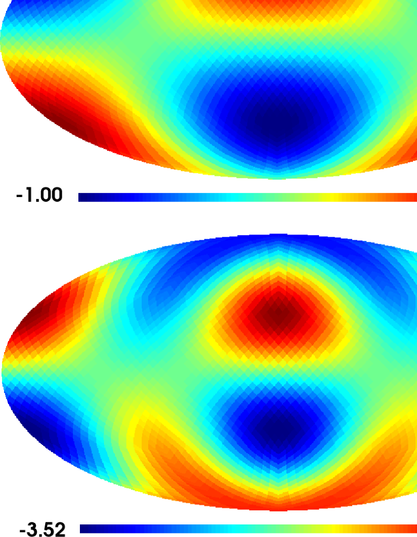
Figure 1: Top panel shows the HEALPIx map of $(\Delta T/T)\times 10^{5}$ for the vector mode [1] (see text). Middle (bottom) panel displays the quadrupole (octopole) of this map. The alignment of $C_{2}$ and $C_{3}$ is evident. The octopole looks planar. Normalization is irrelevant.

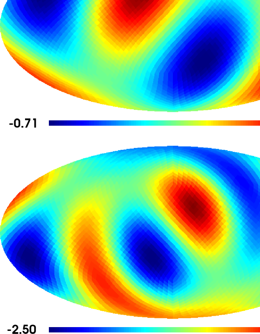
Figure 2: Same as in Fig. 1 for vector mode [2] (see text). There is no alignment in this case, but the octopole is visibly planar. Vectors $\vec{n}_{2}$ and $\vec{n}_{3}$ are almost orthogonal

The value $k_{u}=2\pi/L_{u}$ with $L_{u}=4\times 10^{4}\ Mpc$ has been fixed and, then, for $A=C=0$ and $B=D=6.6\times 10^{-10}$ (mode [1]), vectors $\vec{n}_{2}$ and $\vec{n}_{3}$ appear to be perfectly aligned in the direction (0,1,0) and the octopole is rather planar ($t=0.93$). The total $\Delta T/T$ map is displayed in the top panel of Fig. 1. The central and bottom panels of the same figure show the quadrupolar and octopolar components of this map. Figure 2 has the same structure but it corresponds to $A=B=-C=D=3.3\times 10^{-10}$ (mode [2]). In this last case, there is no alignment. The angle formed by the vectors $\vec{n}_{2}=(0.037,0.706,0.707)$ and $\vec{n}_{3}=(-0.037,0.706,-0.707)$ is very close to $90^{\circ}$ and parameter $t$ takes on the value $t=0.93$ (as in the first case). Other angles and $t$ values appear for other choices of parameters $A,B,C$ and $D$. These results strongly suggest that random superimpositions of arbitrary vector modes should not lead to aligned $\vec{n}_{2}$ and $\vec{n}_{3}$ vectors. This fact is verified in next section by considering a rather general 3D superimposition.

Finally, another type of vector modes (hereafter called $w$-modes) deserves particular attention (see § 5 for applications). In this case, the coordinate axis in momentum space are chosen in such a way that $\vec{k}_{u}=(k_{u1},k_{u2},0)$ and, then, the conditions $v_{cu}^{+}=v_{cu}^{-}=v_{cu}$ are assumed. Complex number $v_{cu}$ can be put in the form $v_{cu}=|v_{cu}|\cos{\beta}+i\,|v_{cu}|\sin{\beta}$. Similarly, we can write $k_{u1}=\sigma_{u}\cos{\alpha}$ and $k_{u2}=\sigma_{u}\sin{\alpha}$. The effect of an unique $w$-mode is now considered. By performing the same kind of calculations as for previous isolated modes, one easily get:

$$W_{x}=W_{y}=0$$ (23)

$$W_{z}=2\sqrt{2}\sigma_{u}|v_{cu}|\,\,(\cos{\beta}\cos{\xi}-\sin{\beta}\sin{\xi})\ ,$$ (24)

where $\xi=\vec{k}_{u}\cdot\vec{r}=\,\sigma_{u}\,r\,(n^{1}\cos{\alpha}+n^{2}\sin{\alpha})$. Furthermore, the associated temperature contrast is:

$$\frac{\Delta T}{T}=\frac{12\sqrt{2}H_{0}^{2}\Omega_{m}|v_{cu}|}{\sigma_{u}}\Big{[}I_{c}\cos{\beta}-I_{s}\sin{\beta}\Big{]}\Big{[}(n^{2}n^{2}-n^{1}n^{1})\frac{\sin{2\alpha}}{2}+n^{1}n^{2}\cos{2\alpha}\,\Big{]}\ .$$ (25)

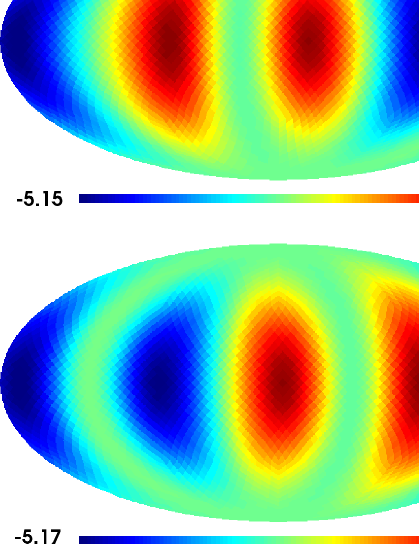
Figure 3: Each panel shows the HEALPIx map of $(\Delta T/T)\times 10^{5}$ produced by a different $w$-mode (see text). The equatorial alignment and the planar character of the octopole are evident in the three panels. Normalization is irrelevant.

Thousands of maps, $M_{i}$, corresponding to different values of $\alpha$ and $\beta$ have been obtained and analyzed. Parameters $\sigma_{u}$ and $|v_{cu}|$ have been fixed. Their values are $\sigma_{u}=\pi/(2\times 10^{4})\ Mpc^{-1}$ and $|v_{cu}|=3.3\times 10^{-10}$. In Fig. 3 we display three of these maps corresponding to distinct $w$-modes; they are different, but the spots are always aligned along the equatorial zone and, consequently, as it has been verified, vectors $\vec{n}_{2}$ and $\vec{n}_{3}$ are aligned along the direction $(0,0,1)$ and, moreover, the octopole is very planar $t\simeq 0.94$. This type of alignment and a high $t$ value (planar octopole) appear in all the maps. Other values of $\sigma_{u}$ and $|v_{cu}|$ have been considered with the same result. If we superimpose many of these maps, the vectors $\vec{n}_{2}$ and $\vec{n}_{3}$ of the resulting map are not always aligned; in other words, any combination of linear modes lying in the plane $(k_{1},k_{2})$ with $v_{c0}^{+}=v_{c0}^{-}=v_{c0}$ does not lead to multipole alignments.

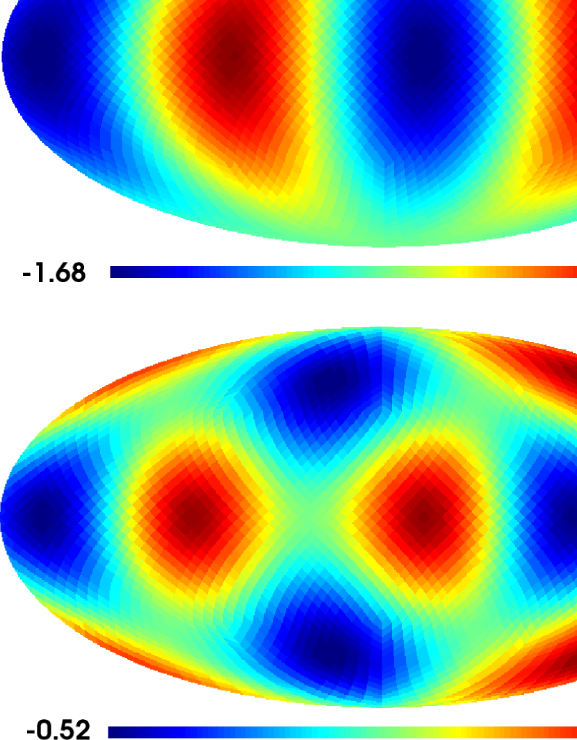
Figure 4: Same as in Fig 1 for the superimposition of $w$-modes $N_{1126}$ (see § 3). Vector $\vec{n}_{2}$ has the direction (0,0,1) and the octopole is not planar. Calculations indicate that vectors $\vec{n}_{2}$ and $\vec{n}_{3}$ are orthogonal; hence, direction $\vec{n}_{3}$ is contained in the equatorial plane. Normalization is irrelevant.

This fact is not surprising taking into account that, for a given map, directions $\vec{n}_{2}$ and $\vec{n}_{3}$ maximize the quantity $\Psi$ defined in Eq. (1), which is nonlinear with respect to the $a_{\ell m}$ coefficients. Superimpositions of $w$-modes have been numerically analyzed in a simple way, we have taken 1521 maps $M_{i}$ and, then, other 1521 maps $N_{j}$ have been obtained according to the following formula: $N_{j}=\sum_{i=1}^{j}M_{i}$. From the analysis of the $N_{j}$ maps, the following conclusions have been obtained: (i) vectors $\vec{n}_{2}$ and $\vec{n}_{3}$ are aligned in the direction (0,0,1) for 1314 of these maps, which appear to have rather planar octopoles, (ii) in the remaining 207 cases, there are no alignments and the octopole is less planar. In Fig. 4, one of these cases is displayed, the spots of the bottom panel are not aligned in the equatorial zone ($t=0.46$) and, then, the direction $\vec{n}_{3}$ is not parallel to (0,0,1). Indeed, it has been numerically verified that these directions are almost orthogonal to (0,0,1) in most of the above $207$ cases. A theoretical proof of this orthogonality is not easy as a result of the particular form of the nonlinear definition of $\vec{n}_{2}$, $\vec{n}_{3}$, and $t$. In § 5, this type of vector modes ($w$-modes) will be superimposed to simulate differential rotations and other symmetric divergenceless motions. Then, the fraction of the superimpositions leading to $\vec{n}_{2}$ and $\vec{n}_{3}$ alignments will be experimentally found.

4 3D superimpositions of vector modes

According to Eq. (9), functions $F_{pq}(\vec{r})$ can be calculated by using the 3D Fast Fourier Transform (FFT). In order to do that, $512^{3}$ cells are considered inside a big box with a size of $2\times 10^{5}\ Mpc$. In this way, the cell size is $\sim 390\ Mpc$ and, consequently, vector modes with spatial scales between $10^{4}\ Mpc$ and $5\times 10^{4}\ Mpc$ can be well described in the simulation. We can then calculate function $F(\vec{r})$ to perform the integral in Eq. (8); in order to do that, the observer is placed at an arbitrary point located in the central part of the simulation box, where the Fourier transform is expected to be well calculated and, then, the integration is performed for each of the $3072$ directions of the pixel centers. The variations of $F(\vec{r})$ along the photon trajectories are smooth and, consequently, the integrations giving $\Delta T/T$ can be easily performed. Furthermore, in a central cube with $1.2\times 10^{5}\ Mpc$ per edge ($60$ % of the box size in our simulations), we can place $5^{3}$ observers uniformly distributed and separated by a distance of $3\times 10^{4}\ Mpc$. Then, quantity $\Delta T/T$ can be calculated for each of these observers; thus, from a given simulation, the information we obtain is greater than in the case of one unique observer located, e.g., at the box center.

In this section, it is assumed (as in paper I) that $v^{\pm}_{c0R}$ and $v^{\pm}_{c0I}$ are four statistically independent Gaussian variables with vanishing mean, and also that each of these numbers has the same power spectrum. The form of this common spectrum is $P(k)=Ak^{n_{v}}$, where $n_{v}$ is the spectral index of the vector modes and $A$ is a normalization constant. Two values of the spectral index: $n_{v}=1$ and $n_{v}=2$ have been considered. The spatial scales are varied from $10^{4}\ Mpc$ to $5\times 10^{4}\ Mpc$ in all cases (only very small wavenumbers are considered). Four realizations of this 3D random superimposition of vector modes have been performed for each spectrum and, then, 125 observers have been located as described above in each of the simulation boxes. Thus, $500$ simulations of the CMB relative temperature variations obtained from the last term of Eq. (3) have been obtained. Moreover, the corresponding $500$ simulations of the term $-\vec{v}_{ce}\cdot\vec{n}$ have been also found. In all cases, linearity conditions $|\vec{h}(\vec{r})|<<<1$ and $|\vec{v}_{c}(\vec{r})|<<<1$) have been verified using the relations:

$$\vec{h}(\eta,\vec{r})=-6H_{0}^{2}\Omega_{m}\,a^{-2}(\eta)\,\int\frac{v_{c0}^{\pm}(\vec{k})}{k^{2}}\,\vec{\epsilon}^{\,\pm}(\vec{\kappa})\exp(i\vec{k}\cdot\vec{r})\,d^{3}k$$ (26)

and

$$\vec{v}^{\pm}_{c}(\eta,\vec{r})=a^{-1}(\eta)\int v_{c0}^{\pm}(\vec{k})\,\vec{\epsilon}^{\,\pm}(\vec{\kappa})\exp(i\vec{k}\cdot\vec{r})\,d^{3}k.$$ (27)

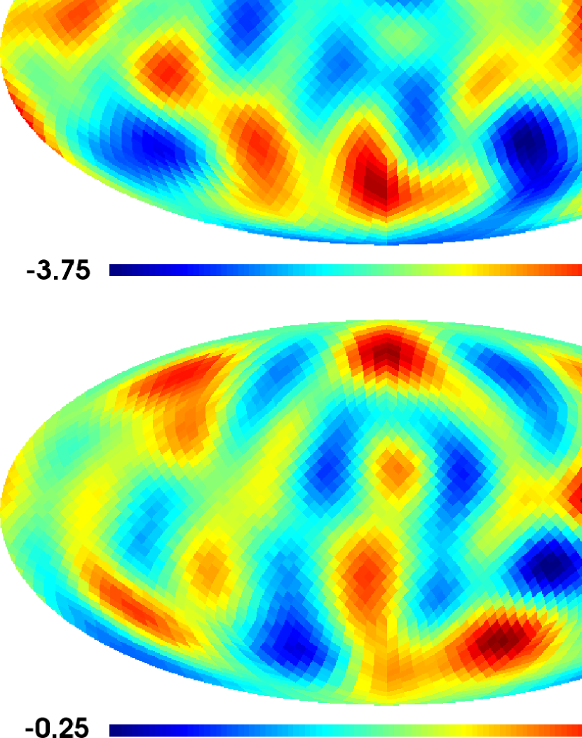
Figure 5: Both panels are HEALPIx maps of quantity $(\Delta T/T)\times 10^{5}$. Top panel shows the part of this quantity due to the last term of Eq. (3), whereas the part obtained from the term $-\vec{v}_{ce}\cdot\vec{n}$ is displayed in the bottom panel. The second part is much smaller than the first one. That is independent on the power spectrum normalization.

The analysis of all these simulations have let to the following main results: (i) the term $-\vec{v}_{ce}\cdot\vec{n}$ is negligible against the last term of Eq. (3). In Fig. 5, we present one simulation of each of these terms for $n_{v}=1$. Numbers in the bottom panel ($-\vec{v}_{ce}\cdot\vec{n}$ term) are much smaller than those of the top panel [last term of Eq. (3)]. Obviously, this comparison is independent on the spectrum normalization. We have verified that the average $\langle C_{2}\rangle$ corresponding to the $500$ maps of the term $-\vec{v}_{ce}\cdot\vec{n}$ is $\sim 1/600$ times smaller than the average calculated from Eqs. (8)–(9); therefore, the term $-\vec{v}_{ce}\cdot\vec{n}$ is hereafter neglected and our study is restricted to the maps obtained from Eqs. (8)–(9); (ii) the angle $\alpha_{23}$ subtended by directions $\vec{n}_{2}$ and $\vec{n}_{3}$ is smaller than $10^{\circ}$ in nine of the $500$ simulations for both spectral indexes: $n_{v}=1$ and $n_{v}=2$. These numbers are compatible with the $8.33$ cases expected for a random distribution of direction $\vec{n}_{3}$ around a fixed $\vec{n}_{2}$ (see de Oliveira-Costa et al. (2004)); (iii) parameter $t$ appears to be greater than $0.94$ in $40$ and $42$ simulations in the cases $n_{v}=1$ and $n_{v}=2$, respectively. These numbers are to be compared with $35$, which is the corresponding number obtained by de Oliveira-Costa et al. (2004) in the case of an isotropic Gaussian random field. All these considerations are independent on the normalization of the spectra.

We can conclude that 3D random superimpositions of large scale vector models do not explain either the observed alignment of $C_{2}$ and $C_{3}$ ($\alpha_{23}\simeq 10^{\circ}$) or the unusually planar octopole ($t\simeq 0.94$). However, the study of some 2D distributions of modes is worthwhile.

5 2D superimpositions of vector modes

Special superimposition of vector modes are now considered. They are 2D superimpositions leading to divergenceless motions in long sized zones, which are hereafter called parallel vorticity regions (PVRs). In each of these regions there is a privileged direction. Inside the region, the angular velocity (describing the local vorticity there) is parallel to the privileged direction everywhere. The $x_{3}$-axis (hereafter $z$-axis) can be chosen to be parallel to the privileged direction. Finally, the PVRs are assumed to be uniform along this axis in the sense that all the orthogonal planes are equivalent. In short, inside the PVRs, the components of the angular velocity are $W_{x}=0$, $W_{y}=0$ and $W_{z}=W_{z}(x^{1},x^{2})$. This configuration appears if functions $v_{c0}^{\pm}(\vec{k})$ are chosen as follows:

$$v_{c0}^{+}(\vec{k})=v_{c0}^{-}(\vec{k})=v_{c0}(\vec{k})\,\delta(\theta_{k}-\frac{\pi}{2})\ .$$ (28)

In this equation, angle $\theta_{k}$ is one of the spherical coordinates in momentum space ($k$ and $\phi_{k}$ being the other two) and $\delta$ stands for the Dirac distribution. By substituting the distributions in Eq. (28) into Eqs. (12)–(14), the following relations are obtained in position space:

$$W_{x}=W_{y}=0$$ (29)

$$W_{z}(x_{1},x_{2})=\sqrt{2}\int v_{c0}(k_{1},k_{2},0)\,\sigma^{2}e^{i(k_{1}x_{1}+k_{2}x_{2})}\,dk_{1}\,dk_{2}\ .$$ (30)

Analogously, from Eqs. (28) and (9), the non-vanishing components of $F_{pq}$ appear to be:

$$F_{11}=-F_{22}=-\sqrt{2}\int\frac{k_{1}k_{2}}{\sigma^{2}}\,v_{c0}(k_{1},k_{2},0)\,e^{i(k_{1}x_{1}+k_{2}x_{2})}\,dk_{1}\,dk_{2}\ ,$$ (31)

$$F_{12}=\sqrt{2}\int\frac{k_{1}^{2}}{\sigma^{2}}\,v_{c0}(k_{1},k_{2},0)\,e^{i(k_{1}x_{1}+k_{2}x_{2})}\,dk_{1}\,dk_{2}\ ,$$ (32)

$$F_{21}=-\sqrt{2}\int\frac{k_{2}^{2}}{\sigma^{2}}\,v_{c0}(k_{1},k_{2},0)\,e^{i(k_{1}x_{1}+k_{2}x_{2})}\,dk_{1}\,dk_{2}\ .$$ (33)

Finally, vector $\vec{G}(\vec{r})$ involved in Eqs. (10)–(11) has the following components:

$$G_{x}=G_{y}=0$$ (34)

$$G_{z}(x_{1},x_{2})=-\sqrt{2}\int v_{c0}(k_{1},k_{2},0)\,e^{i(k_{1}x_{1}+k_{2}x_{2})}\,dk_{1}\,dk_{2}\ .$$ (35)

As it follows from Eq. (28), our 2D superimpositions are combinations of the $w$-modes studied at the end of § 3 ($k_{3}=0$ and $v_{c0}^{+}=v_{c0}^{-}=v_{c0}$) and, consequently, vectors $\vec{n}_{2}$ and $\vec{n}_{3}$ are expected to be either parallel or orthogonal (almost in all cases). The proportions between alignments and no alignments will be numerically obtained from the analysis of simulations.

5.1 Differential rotations

A present angular velocity of the form $W_{z}=W_{z}(\rho)$ is assumed, where $\rho=\sqrt{x_{1}^{2}+x_{2}^{2}}$. This velocity describes a particular PVR, which could be interpreted as a big region undergoing a differential rotation. The local vorticity only depends on the distance to the $z$-axis, which plays the role of the rotation axis. Then, from Eq. (30) one easily finds

$$v_{c0}(k_{1},k_{2},0)=\frac{\sqrt{2}}{8\,\pi^{2}\,\sigma^{2}}\int W_{z}(\rho)\,e^{-i(k_{1}x_{1}+k_{2}x_{2})}\,dx_{1}\,dx_{2}\ .$$ (36)

Function $v_{c0}(k_{1},k_{2},0)$ is calculated by using the last equation and, then, this function is substituted into Eqs. (31)–(33), to get the $F_{pq}$ components. It is also substituted into Eq. (35) to obtain $G_{z}$. All these functions only depend on the coordinates $x_{1}$ and $x_{2}$. They are easily extended inside a 3D cube (where photons move) taking into account that the planes orthogonal to the $z$-axis are indistinguishable. For example, in the case of function $F_{12}$, its value at any point with coordinates $(x^{1},x^{2},x^{3})$ located inside the 3D cube would be $F_{12}(x^{1},x^{2},x^{3})=F_{12}(x^{1},x^{2},0)$. These extended functions allow us to calculate either $\Delta T/T$ (from Eq. (8)) or the polarization rotation angle $\delta\psi$ (from Eq. (10)). These calculations can be performed for any observer located well inside the cube; in other words, for any observer whose last scattering surface is fully localized inside the cube.

It is worthwhile to notice that, in the case of the rigid rotation of a big region, the angular velocity $W_{z}$ vanish in a certain gauge, in which the observer rotates with the region. In this gauge, Eq. (36) gives: $v_{c}(k_{1},k_{2},0)=0$ and, taking into account that this quantity is gauge invariant, it vanishes in any gauge; therefore, according to Eqs. (31)–(35) plus Eqs. (8) and (10), quantities $\Delta T/T$ and $\delta\psi$ vanish. In short, there is no either CMB anisotropy or Skrotskii rotations associated to rigid rotations (the same is valid for rotations of the spatial coordinates in the absence of vector modes). These effects only appear in the case of differential rotations, which cannot be globally avoided by any rotation of the reference frame.

Two functions $W_{z}=W_{z}(\rho)$ have been used: the first one is

$$W^{{}^{N}}_{z}(\rho)=\cases{N_{1}\Big{[}e^{-(\rho^{2}/2m^{2})}-e^{-2}\Big{]}&\,\,\,\,\, $\rho\leq 2m$\cr 0&\,\,\,\,\, $\rho>2m$\cr}\ ,$$ (37)

where $N_{1}$ is a normalization constant. The length $m$ defines the spatial size of the PVR. The values $m=5\times 10^{3}\ Mpc$ (case NI) and $m=3\times 10^{3}\ Mpc$ (case NII) have been tried. Evidently, the spatial scales involved in this differential rotation are very large. The second function is:

$$W^{{}^{C}}_{z}(\rho)=\cases{N_{2}\cos{(\pi\rho/2\rho_{max})}&\,\,\,\, $\rho\leq\rho_{max}$\cr 0&\,\,\,\, $\rho>\rho_{max}$\cr}\ ;$$ (38)

quantities $N_{2}$ and $\rho_{max}$ being the normalization constant and the parameter defining the spatial profile of the angular velocity, respectively. Two values of $\rho_{max}$ have been studied: $\rho_{max}=6.8\times 10^{3}\ Mpc$ (case CI) and $\rho_{max}=4\times 10^{3}\ Mpc$ (case CII).

Once an angular velocity profile $W_{z}=W_{z}(\rho)$ has been assumed (cases NI, NII, CI, and CII), only two elements remain free: (i) the normalization constant, and (ii) the location of the observer in the simulation square. The square is that appropriate for the Fourier transforms in Eqs. (31)–(35). For the above profiles, a square size of $5\times 10^{4}\ Mpc$ is used and, then, 81 observers are uniformly located in a central square of $2\times 10^{4}\ Mpc$ size. The separation between neighboring observers is $2.5\times 10^{3}\ Mpc$; therefore, once parameter $m$ ($\rho_{max}$) is fixed in the profile $W^{{}^{N}}_{z}$ ($W^{{}^{C}}_{z}$), $81$ simulations of $\Delta T/T$ and $\delta\psi$ can be obtained as it has been described in the first paragraph of § 5.1. Each map corresponds to a localization of the observer characterized by its distance to the rotation axis ($x_{1}=x_{2}=0$ line). The analysis of the resulting HEALPIx maps has let to the following main conclusions: (1) the $C_{2}$-$C_{3}$ alignment is perfect for any of the above $W_{z}$ profiles and observers ($\alpha_{23}=0$), (2) the inequality $t>0.94$ also is satisfied in all cases. These results are encouraging. The proposed differential rotations plus appropriate large scale scalar modes could easily lead to the observed angle $\alpha_{23}\simeq 10^{\circ}$ and also to the parameter $t\simeq 0.94$. Of course, the large scale vector modes under consideration should dominate against the scalar ones. Thus, the alignment produced by the differential rotation (vector modes) would not be hidden by the effects of standard scalar modes. The amplitude of the scalar perturbations contributing to small $\ell$ multipoles (very large scales) should be smaller than those corresponding to the standard flat spectrum (compatible with the remaining observed $C_{\ell}$ quantities). Either a certain cutoff or a damping of the scalar fluctuations would be necessary on very large scales. Details about the possible cutoff scale or the gradual damping are out of the scope of this paper; however, the general considerations of this paragraph are important to normalize the $W_{z}$ profiles.

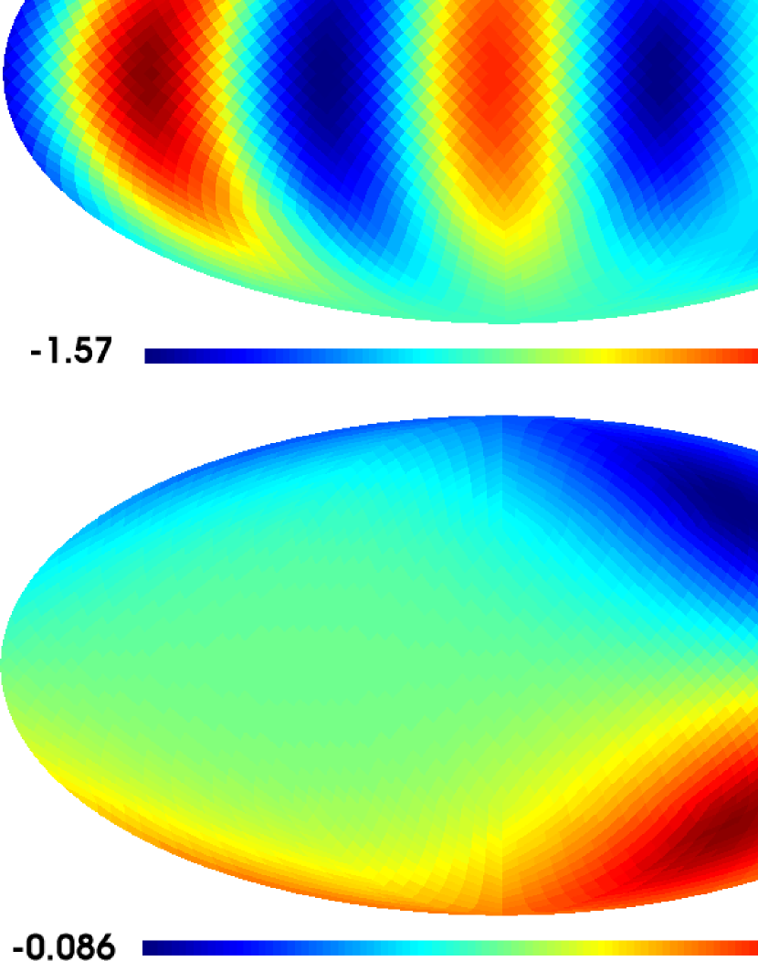
Figure 6: Top panel is a HEALPIx map of $(\Delta T/T)\times 10^{5}$ for case NI and observer $i=1$ (see Table 1). A strong $C_{2}$–$C_{3}$ alignment and a high $t$ value are evident. The corresponding $\delta\psi$ map is displayed in the bottom panel, where the angles are given in degrees.

A few considerations about recent CMB observations are necessary before describing our normalization method. According to Hinshaw et al. (2006) (WMAP three years data analysis), the CMB quadrupole is $C^{{}^{WMAP}}_{2}\simeq 2.96\times 10^{-11}$ whereas the octopole is $C^{{}^{WMAP}}_{3}\simeq 7.38\times 10^{-11}$; hence, if it is assumed that the contribution of scalar and vector modes to these multipoles are to be added (statistical independence of the scalar modes and the differential rotation) and, moreover, it is taken into account that the contribution of the vector modes must dominate (see previous paragraph), such a vector contribution should roughly satisfy the following conditions: (a) $C_{2}$ must be a little smaller than $2.96\times 10^{-11}$ and, (b) $2C_{2}<C_{3}<3C_{2}$; hence, the following method is used to normalize in each of the cases NI, NII, CI, and CII: in a first step, the $C_{2}$ and $C_{3}$ multipoles of the 81 maps are calculated for an arbitrary normalization and, then, the maps (observers) compatible with condition (b) –which is independent on normalization– are found. The total number, $N_{b}$, of these maps is given –for each case– in Table 1. Some of these maps correspond to observers located at the same distance from the rotation axis and, consequently, their normalizations are identical except for small numerical errors. This fact has been verified. The total number of distinct distances (observers), $N_{d}$, and the distances themselves, $d_{or}(i)$ with $i:1,N_{d}$, are also given in Table 1. In a second step, the normalization constant is chosen to have $C_{2}=2.5\times 10^{-11}$ for each of the above $N_{d}$ observers and, then, the resulting octopoles, $C_{3}(i)$, are calculated and shown in Table 1 for $i:1,N_{d}$. A number $N_{d}$ of different normalizations is thus obtained. Each of these normalizations is separately considered. The $\Delta T/T$ and $\delta\psi$ maps corresponding to one of the two observers of case NI ($i=1$ in Table 1) are displayed in Fig. 6. Top panel shows a $\Delta T/T$ map which seems to be clearly compatible with a planar octopole (estimated value: $t\simeq 0.9979$) and a perfect alignment ($\alpha_{23}=0$, with possible small errors due to the limited angular resolution of the HEALPIx maps). Bottom panel displays the corresponding $\delta\psi$ map. Angles close to $0.1$ degrees are reached in some directions, the angles are similar (a little smaller) than those obtained in paper I, which were estimated by using a rather arbitrary normalization.

Table 1: 2D simulations based on $W_{z}$ profiles.

CASE	$N_{b}$	$N_{d}$	$C_{3}(1)\times 10^{11}$	$C_{3}(2)\times 10^{11}$	$d_{or}(1)\times 10^{-3}$	$d_{or}(2)\times 10^{-3}$	$A_{wz}(1)\times 10^{9}$	$A_{wz}(2)\times 10^{9}$
NI	12	2	$7.23$	$5.94$	$7.9\ Mpc$	$9.0\ Mpc$	$0.99$	$0.95$
NII	8	1	$6.58$	–	$7.9\ Mpc$	–	$2.51$	–
CI	12	2	$7.04$	$5.33$	$7.9\ Mpc$	$9.0\ Mpc$	$1.51$	$1.41$
CII	8	1	$5.77$	–	$7.9\ Mpc$	–	$3.94$	–

Note. — First column lists the four $W_{z}$ profiles defined in the text. In each case, 81 observers are uniformly distributed in the central part of the simulation box

Note. — $C_{3}(1)$ is the octopole (after normalization by the condition $C_{2}=2.5\times 10^{-11}$) of one of the $N_{d}$ observers, whereas $C_{3}(2)$ corresponds to the second of these observers (if it exists). The same for $d_{or}$ and for the dimensionless ratio $W_{z}(\rho=0)/H_{0}$

After the above normalization method has been applied, any of the $N_{d}$ normalizations corresponds to an observer (characterized by its distance to the rotation center) whose $C_{2}$ and $C_{3}$ multipoles satisfy the following conditions: (i) they are appropriate to explain the values observed by the WMAP satellite with the help of a certain contribution due to scalar modes (to be estimated), (ii) these multipoles are fully aligned, and (iii) the octopole is very planar ($t>0.94$). The distances from the observers to the rotation axis are different from zero (see Table 1) and, consequently, these observers are not placed on the rotation axis but in another position, which is so much probable as any other position in the space.

Normalizations lead to the values of the constants $N_{1}$ and $N_{2}$ involved in Eqs. (37)–(38), from which, the dimensionless amplitude of the angular velocity profile $A_{wz}=W_{z}(\rho=0)/H_{0}$ can be found in each case. The resulting $A_{wz}$ values are given in Table 1 for the normalizations included in it. They are a few times greater than the value $4.3\times 10^{-10}$ reported by (Jaffe et al., 2005) in the framework of a fully different model.

5.2 Statistical parallel vorticity fields

In this section, a PVR region is simulated by using statistical methods. The components $v_{c0R}$ and $v_{c0I}$ of the complex numbers $v_{c0}(k_{1},k_{2},0)$ are generated as two statistically independent Gaussian variables with the same power spectrum and zero mean. The form of the spectrum is the same as in the 3D simulations; namely, $P(\sigma)=A\sigma^{n_{v}}$, and the chosen spectral indexes and spatial scales are also the same as in the 3D statistical realizations.

Ten realizations of these 2D random superimposition of vector modes have been performed for each spectrum ($n_{v}=1$ and $n_{v}=2$) and, then, 81 observers have been uniformly located in the simulation square using the same method as in the 2D simulations with $W_{z}$ profiles; however, the sizes of the simulation square and the central square are $2\times 10^{5}\ Mpc$ and $1.28\times 10^{5}\ Mpc$, respectively, and the distance between observers is $1.6\times 10^{3}\ Mpc$. Thus, $810$ simulations of the CMB relative temperature variations produced by PVRs have been obtained. The corresponding $\delta\psi$ maps have been also found. All these maps have been analyzed. Results from this analysis are now described; we begin with various conclusions which are independent on the spectrum normalizations: ($\alpha$) the angle $\alpha_{23}$ is zero in the $48.64\%$ ($48.4\%$) of the $810$ simulations for $n_{v}=1$ ($n_{v}=2$), ($\beta$) parameter $t$ appears to be greater than $0.94$ in the $18.64\%$ ($19.88\%$) of the simulations for $n_{v}=1$ ($n_{v}=2$), and ($\gamma$) the conditions $t>0.94$ and $\alpha_{23}=0$ are simultaneously satisfied in the $\sim 11\%$ ($\sim 12\%$) of the simulations for $n_{v}=1$ ($n_{v}=2$). These last percentages can be found from Table 2, where the number of cases, $n_{at}$, satisfying the two relations $t>0.94$ and $\alpha_{23}=0$ is given for each of the ten 2D realizations. We have counted these cases because, as it has been discussed in § 3, conditions $t>0.94$ and $\alpha_{23}=0$ do not seem to be independent and, consequently, the probability of the realizations satisfying the two relations is not a priori the product of the individual probabilities.

The spectra are normalized as follows: first, all the simulations satisfying the conditions $t>0.94$ and $\alpha_{23}=0$ are normalized by the condition $C_{2}=2.5\times 10^{-11}$ and, then, those of them satisfying the inequalities $2C_{2}<C_{3}<3C_{2}$ are identified and counted. Their total number, $n_{obs}$, is given in Table 2 for each of our ten 2D realization. It is worthwhile to notice that, each of the normalized simulations corresponds to one of the ten 2D statistical realizations and also to an observer located at a certain position in the simulation cube. Since there is no a rotation axis, coordinates $x^{1}$ and $x^{2}$ are both necessary to fix the observer position in the plane orthogonal to the vorticity direction of the PVR.

For $n_{v}=1$ ($n_{v}=2$), number $n_{obs}$ appears to be zero in five (one) of our ten 2D statistical superimpositions of vector modes. In these five (one) cases, conditions $t>0.94$ and $\alpha_{23}=0$ are satisfied (see Table 2), but there are no observers measuring a quadrupole $C_{2}=2.5\times 10^{-11}$ and an octopole satisfying the relations $2C_{2}<C_{3}<3C_{2}$. It is then easily calculated the probability of having at least an observer whose measurements satisfy the four conditions $t>0.94$, $\alpha_{23}=0$, $C_{2}=2.5\times 10^{-11}$ and, $2C_{2}<C_{3}<3C_{2}$, namely, whose measurements may be compatible with current observations after introducing appropriate sub-dominant scalar modes. This probability is close to $\sim 5.5\%$ ($\sim 10.8\%$) for $n_{v}=1$ ($n_{v}=2$). With these probabilities we cannot say that we live in a very special zone of the PVR, but in a reasonably probable one, which is equally probable than any other positions inside the PVR.

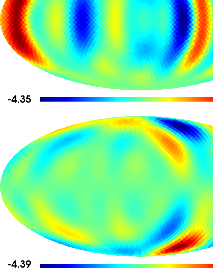
Figure 7: Top: same as in Fig. 6 for one of the two observers measuring multipoles $C_{2}$ and $C_{3}$ compatible with current observations in the realization number $9$ of the case $n_{v}=2$ (see Table 2 and text). Bottom: the corresponding Skrotskii angles, $\delta\psi$, are given in units of $10^{-3}$ degrees.

For $n_{v}=2$ and the 2D realization number $9$ of Table 2, there are two observers ($n_{obs}=2$) whose measurements are compatible with the four above conditions. One of these observers, located at $\sim 5\times 10^{4}\ Mpc$ from the cube center, would measure $t\simeq 0.9631$, $\alpha_{23}=0$, $C_{2}=2.5\times 10^{-11}$, and $C_{3}=6.45\times 10^{-11}$. The $\Delta T/T$ and $\delta\psi$ maps corresponding to this observer are shown in Fig. 7. Top panel displays the $\Delta T/T$ map, which looks like those compatible with a planar octopole and a perfect alignment. The corresponding $\delta\psi$ map is exhibited in the bottom panel. The largest angles – close to $\sim 4.4\times 10^{-3}$ degrees– are much smaller (by a factor $\sim 1/50$) than those based on the normalization of paper I. Of course, these angles are too small to produce any currently significant $B$-polarization of the CMB.

Table 2: Statistical 2D simulations.

CASES ($n_{v}=1$)	$n_{at}$	$n_{obs}$	CASES ($n_{v}=2$)	$n_{at}$	$n_{obs}$
1	7	1	1	11	3
2	9	0	2	10	1
3	6	2	3	12	2
4	9	1	4	12	2
5	9	0	5	11	2
6	7	3	6	10	1
7	9	0	7	12	2
8	4	0	8	12	1
9	11	1	9	12	2
10	17	0	10	12	0

Note. — Ten 2D statistical simulations corresponding to the spectral indexes $n_{v}=1$ and $n_{v}=2$ are numbered in the first and fourth columns, respectively

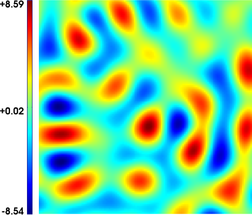
Figure 8: Map of the dimensionless quantity $(W_{z}/H)_{0}\times 10^{9}$ in the plane orthogonal to the angular velocity. The size of the represented square is $50\ Mpc$

Finally, Fig. 8 shows a dimensionless quantity proportional to the present angular velocity $W_{z}$. The represented zone is located inside the simulation square and centered in it. The normalization is the same as in Fig. 7 (same 2D simulation and observer). Red and blue spots correspond to regions which are rotating in opposite senses. A boundary with $W_{z}=0$ separates them. The mean value of $(W_{z}/H)_{0}$ is negligible by construction and the typical deviation is $\langle|W_{z}|^{2}\rangle^{1/2}/H_{0}=3.\times 10^{-9}$. Many realizations (as that of the Figure) have been considered to conclude that the typical value of $(W_{z}/H)_{0}$ is always a few times $10^{-9}$.

6 Discussion and conclusions

Appropriate combinations of large scale vector perturbations have been introduced in the concordance model and, then, their effects on the CMB anisotropy have been studied in detail. Our main conclusions can be summarized as follows: 3D superimpositions of vector modes do not explain the CMB anomalies; however, some 2D superimpositions of these modes lead to good results. Two types of 2D simulations have been performed: one of them represents differential rotations of big regions and the other one leads to extended statistical PVRs. In these two cases there is a preferred direction of symmetry. It is the direction of the angular velocity, which is the same in any point of the perturbed region. In the first case, there is a symmetry around the rotation axis in the plane orthogonal to the preferred direction, however, statistical PVRs do not introduce such a rotational symmetry.

Suitable differential rotations can explain the planar character of the octopole, its alignment with the quadrupole, and the main part of the $C_{2}$ and $C_{3}$ values observed with WMAP. These facts are proved, in § 5.1, for two different $W_{z}$ profiles. Polarization rotation angles $\delta\psi$ close to $0.1$ degrees are produced by these profiles. Other possible profiles could produce slightly greater angles. A sub-dominant contribution of large scale scalar modes could then account for a small part of the observed quadrupole and octopole, which would be complementary of the part due to vector modes. These scalar modes could be also responsible for the observed angle $\alpha_{23}\simeq 10^{\circ}$, which vanishes for pure differential rotations. The required scalar modes would destroy the rotational symmetry in the plane orthogonal to the axis of the differential rotation. Skrotskii rotations close to $0.1$ degrees would produce a $B$-polarization of the CMB, which could be marginally observable by future satellites (see paper I).

For statistical PVRs, there is an appreciable probability of accounting for all the anomalies explained by differential rotations. This probability depends on the form of the assumed power spectrum and also on the interval of $k$ values considered in the computations. The dependence on the spectral index has been pointed out by considering two distinct values $n_{v}=1$ and $n_{v}=2$ (see § 5.2). The mentioned probability is greater in the case $n_{v}=2$ ($\sim 11\%$). Of course, a certain level of scalar modes is necessary (as in the case of differential rotations) in order to explain the observed angle $\alpha_{23}\simeq 10^{\circ}$. Statistical PVRs lead to $\delta\psi$ angles which are too small to produce significant levels of $B$-polarization. Other intervals of spatial scales, and other power spectra could lead to higher probabilities for the explanation of anomalies and, perhaps, to greater Skrotskii rotations. In a certain $k$ interval, the spectrum of vector modes could have any form (a power law is not required either by any theoretical prediction or by observational evidences). In a finite interval, e.g., between $10^{4}$ and $5\times 10^{4}\ Mpc$, the spectral index of a power spectrum is arbitrary, nevertheless, only some spectral indexes are admissible, as $k$ tends to zero, to avoid divergences in some integrals (e.g., that of Eq. (31)).

In Rackić & Schwarz (2007), it is stated that, at high confidence, there is no any rotational symmetry of the CMB in the plane orthogonal to the symmetry axis. This fact is compatible with differential rotations by two reasons: (i) the mentioned rotational symmetry would be only observed from points placed on the rotation axis, whereas we are not located on this line with very high probability, and (ii) there may be either large scale sub-dominant scalar perturbations or deviations with respect to a perfect differential rotation and, obviously, these perturbations and deviations could contribute to hide any rotational symmetry and also to explain the deviation from zero observed in the angle $\alpha_{23}$.

The asymmetry of the the North and South ecliptic hemispheres is also compatible with our 2D superimpositions of vector modes. We predict two equivalent hemispheres, nevertheless, they are not separated by the ecliptic plane, but by the plane orthogonal to the angular velocity. Furthermore, in some slightly different scenarios, the equivalence of these two hemispheres could disappear. It occurs, e.g., if the last scattering surface of the observer is partially outside the PVR, which is particularly probable for PVRs which are not too extended in some direction.

Solar system alignments would be casual, as it seems natural in any cosmological explanation of the observed anomalies. See Cho (2007). All the theories of this type (including our proposal) would be ruled out by solutions of the CMB anomaly problem based on both, the ordinary spectrum of scalar perturbations, and a non cosmological component accounting for the observed statistical correlations with the local geometry of the solar system; however, current observations and data analysis have not unveiled any component of this type accounting for the CMB anomalies.

We have assumed very large spatial scales to alter only a few low-$\ell$ multipoles; nevertheless, only vector modes have been considered. Why large scale scalar modes have not been tried? The main reasons are now pointed out. For the chosen spatial scales, combinations of modes should lead to very large almost-homogeneous regions. It occurs whatever the nature of the perturbations may be. In the case of vector modes, the angular velocity will be almost-homogeneous in these regions and, consequently, it will have almost the same direction everywhere. These absolutely natural regions, which could have sizes comparable to that of the sphere bounded by the large scattering surface (for large enough spatial scales), are the PVRs we need to explain anomalies. In the case of scalar perturbations, the density contrast should be almost-constant in these large regions and, consequently, a cylindrical scalar inhomogeneity would be actually unlikely. Moreover, a flattened inhomogeneity does not seem likely as a result of the small scales required by the short thickness of the structure, which would be small enough to affect multipoles with too large $\ell$ values. Hence, symmetry axis and preferred planes seem to be rather improbable in the case of large scale scalar modes. Although these arguments are qualitative they strongly suggest the use of vector modes.

Let us finish this paper with a list of a few open problems which should be addressed in the near future: (1) the origin and evolution laws of the vector modes (e.g. brane-worlds, strings, and so on) deserve particular attention. Only a consistent theory on these subjects could give answers to important questions as: in what a cosmological period (or periods) are generated the vector modes? How do they actually decay? How much probable are the PVRs? Are scalar and vector modes statistically independent? (2) Multipole components for $\ell>3$ must be also analyzed and compared with those extracted from WMAP data. Multipole vectors (Copi et al., 2004) should be used in this extended study. (3) The proportions between large scale scalar and vector modes must be considered in more detail and, (4) deviations from the perfect parallelism assumed in our 2D superimpositions of vector modes could lead to interesting results (hemisphere asymmetry, $\alpha_{23}$ observed value, and so on).

Large scale rotations are currently enigmatic (even for us), but the origin of the familiar cosmic expansion has kept unknown during a century. In both cases, rotations and expansion, rejection (acceptance) would be only justified by the disagreement (agreement) between predictions and observations (without prejudices). Although we have not a closed theory on the subject of this paper, results related with the CMB anomalies are actually encouraging and, consequently, more study is worthwhile.

References

- Bardeen (1980) Bardeen, J.M. 1980, Phys. Rev. D, 22, 1882
- Bernui et al. (2007) Bernui, A., Mota, B., Rebouças, M.J., & Tavakol, R., 2007, A@A, 479, 2007
- Bielewicz et al. (2004) Bielewicz, P., Górski, K.M., & Banday, A.J., 2004, MNRAS, 355, 1283
- Bridges et al. (2005) Bridges, M., McEwen, J.D., Lasenby, A.N., & Hobson, M.P., 2005, astro-ph/0605325
- Bunn (2002) Bunn, E.F., 2002, Phys. Rev. D, 65 043003
- Cho (2007) Cho, A., 2007, Science, 317, 1848
- Copi et al. (2004) Copi, C.J., Huterer, D., & Starkman, G.D., 2004, Phys. Rev. D, 70, 043515
- Copi et al. (2006) Copi, C.J., Huterer, D., Schwarz, D.J., & Starkman, G.D., 2006, MNRAS, 367, 79
- Copi et al. (2007) Copi, C.J., Huterer, D., Schwarz, D.J., & Starkman, G.D., 2007, Phys. Rev. D, 75, 023507
- Cruz et al. (2005) Cruz, M., Martínez-González, E., Vielva, P., & Cayón, L., 2005, MNRAS, 356, 29
- de Oliveira-Costa et al. (2004) de Oliveira-Costa, A., Tegmark, M., Zaldarriaga, M., & Hamilton, A., 2004, Phys. Rev. D, 69, 063516
- Efstathiou (2003) Efstathiou, G., MNRAS, 2003, 346, L26
- Efstathiou (2004) Efstathiou, G., MNRAS, 2004, 348, 885
- Eriksen et al. (2004a) Eriksen, H.K., Hansen, F.K., Banday, A.J., Górski, K.M. & Lilje, P.B., 2004, ApJ, 605, 14
- Eriksen et al. (2004b) Eriksen, H.K., Banday, A.J., Górski, K.M. & Lilje, P.B., 2004, ApJ, 612, 633
- Eriksen et al. (2007) Eriksen, H.K., Banday, A.J., Górski, K.M. Hansen, F.K., & Lilje, P.B., 2007, astro-ph/0701089
- Gaztañaga et al. (2003) Gaztañaga, E., Wagg, J., Multamäki, T., Montaña, A., & Hughes, D.H., 2003, MNRAS, 346, 47
- Ghosh et al. (2007) Ghosh, T., Hajian, A., & Souradeep, T., 2007, Phys. Rev. D, 75, 083007
- Górski et al. (1999) Górski, K.M., Hivon, E., & Wandelt, B.D.,: In Proceedings of the (MPA/ESO Conference on Evolution of Large Scale Structure), Eds: A.J. Banday, R.K. Sheth and L. Da Costa (1999) [astro-ph/9812350]
- Hajian (2007) Hajian, A., 2007, astro-ph/0702723
- Hansen et al. (2004a) Hansen, F.K., Banday, A.J., & Górski, K.M., 2004, MNRAS, 354, 641
- Hansen et al. (2004b) Hansen, F.K., Balbi, A., Banday, A.J., & Górski, K.M., 2004, MNRAS, 354, 641
- Hinshaw et al. (2006) Hinshaw, G. et al., 2006, astro-ph/0603451.
- Hu & White (1997) Hu, W., & White, M., 1997, Phys. Rev. D, 56, 596
- Inoue & Silk (2006a) Inoue, K.T., & Silk, J., 2006, ApJ, 648, 23
- Inoue & Silk (2006b) Inoue, K.T., & Silk, J., 2006, astro-ph/0612347
- Jaffe et al. (2005) Jaffe, T.R., Banday, A.J., Eriksen H.K., Górski, K.M., and Hansen, F.K. 2005, ApJ, 629, L1
- Jaffe et al. (2006a) Jaffe, T.R., Banday, A.J., Eriksen H.K., Górski, K.M., and Hansen, F.K. 2006, ApJ, 643, 616
- Jaffe et al. (2006b) Jaffe, T.R., Banday, A.J., Eriksen H.K., Górski, K.M., and Hansen, F.K. 2006, A&A, 460, 393
- Land & Magueijo (2005) Land, K., & Magueijo, J., 2005, Phys. Rev. Lett., 95, 071301
- Land & Magueijo (2006) Land, K., & Magueijo, J., 2006, astro-ph/0611518
- Maartens (2000) Maartens, R. 2000, Phys. Rev. D, 62, 084023
- Martínez-González et al. (2006) Martínez-González, E., Cruz, M., Cayón, L., & Vielva, P., 2006, New Astron. Rev., 50, 875
- Morales & Sáez (2007) Morales, J.A., & Sáez, D. 2007, Phys. Rev. D, 75, 043011
- Rackić & Schwarz (2007) Rackić, A., & Schwarz, D.J., 2007, Phys. Rev. D, 75, 103002
- Schwarz et al. (2004) Schwarz, D.J., Starkman, G.D., Huterer, D., & Copi, C.J., 2004, Phys. Rev. Lett., 93, 221301
- Slosar et al. (2004) Slosar, A., Seljak, U., & Makarov, A., 2004, Phys. Rev. D, 69, 2004
- Skrotskii (1957) Skrotskii, G.V. 1957, Dokl. Akad. Nauk. USSR, 114, 73. Englihs translation: Sov. Phys.–Dokl., 2, 226
- Spergel et al. (2003) Spergel, D.N. et al., 2003, ApJS, 148, 175
- Spergel et al. (2006) Spergel, D.N. et al., 2006, astro-ph/0603449
- Vielva et al. (2004) Vielva, P., Martínez-González, E., Barreiro, R.B., Sanz, J.L., & Cayón, L., 2004, ApJ, 609, 22