Symmetry Classes of Spin and Orbital Ordered States in a $\mathrm{t_{2g}}$ Hubbard Model on a Two-dimensional Squar Lattice

Abstract

This paper presents symmetry classes of the Hartree-Fock (HF) solutions of spin and orbital ordered states in a $\mathrm{t_{2g}}$ Hubbard model on a two-dimensional square lattice. Using a group theoretical bifurcation theory of the Hartree-Fock equation, we obtained many types of broken symmetry solutions which bifurcate from the normal state through one step transition in cases of commensurate ordering vectors $\mbox{\boldmath$Q$}_{0}=(0,0)$, $\mbox{\boldmath$Q$}_{1}=(\pi,\pi)$, $\mbox{\boldmath$Q$}_{2}=(\pi,0)$ and $\mbox{\boldmath$Q$}_{3}=(0,\pi)$. Each broken symmetry state is characterized by the presence of local order parameters(LOP) at each lattice site: quadrupole moment $\mbox{\boldmath$Q$}=(Q_{2}^{2},Q_{12},Q_{23},Q_{31})$, orbital angular momentum $\mbox{\boldmath$l$}=(l_{1},l_{2},l_{3})$, spin density $\mbox{\boldmath$s$}=(s^{1},s^{2},s^{3})$, spin quadrupole moment $\mbox{\boldmath$Q$}^{\lambda}=(Q_{2}^{2\lambda},Q_{12}^{\lambda},Q_{23}^{\lambda},Q_{31}^{\lambda})$ and spin orbital angular momentum $\mbox{\boldmath$l$}^{\lambda}=(l_{1}^{\lambda},l_{2}^{\lambda},l_{3}^{\lambda})$ where $\lambda=1,2,3$. We performed numerical calculations for some parameter sets. Then we have found that many types of non-collinear magnetic orbital ordered states having LOP:$\mbox{\boldmath$Q$}^{\lambda}$ and $\mbox{\boldmath$l$}^{\lambda}$ can be the ground state for these parameter sets.

1 Introduction

Perovskite-type RTiO₃ and RVO₃[1, 2, 3] (R being a rare-earth ion or Y) and quasi two-dimensional ruthenate compounds Ca_2-xSr_xRuO₄ [4, 5, 6, 7, 8] have gained considerable interest because of their plentiful phases including various orbital orders. In a previous paper[9] (hereafter we cite it as I), in order to study these perovskite-type compounds, we have considered a triply degenerate $\mathrm{t_{2g}}$ Hubbard model on a three-dimensional cubic lattice.

In the paper we have presented a brief review of the general group theoretical bifurcation theory of the Hartree-Fock (HF) equation. By listing axial isotropy subgroups of the R-reps(irreducible representation over the real number field) of the group $G_{0}$ of symmetry of the system, we have obtained various types of non magnetic orbital ordered states and collinear magnetic orbital ordered states, which bifrurcate from the normal state through one step transition in the cases of ordering vectors $\mbox{\boldmath$Q$}_{\rm F}=(0,0,0)$ and $\mbox{\boldmath$Q$}_{\rm G}=(\pi,\pi,\pi)$.

In the present paper, to study quasi two-dimensional ruthenate compounds, we consider a three-orbital $\mathrm{t_{2g}}$ Hubbard model on a two-dimensional square lattice[5]. We apply the group theoretical bifurcation theory to this model.

In this paper we consider broken symmetry states with ordering vectors $\mathrm{\Gamma\ point}:\mbox{\boldmath$Q$}_{0}=(0,0)$, $\mathrm{M\ point}:\mbox{\boldmath$Q$}_{1}=(\pi,\pi)$ and $\mathrm{X\ point}:\mbox{\boldmath$Q$}_{2}=(\pi,0)$ and $\mbox{\boldmath$Q$}_{3}=(0,\pi)$ which can allow states with double $Q$. Also we consider magnetic states with non-collinear spin structure, which were not treated in I.

This paper is organized as follows. In §2 we give a model Hamiltonian and its symmetry group $G_{0}$. In §3 we present a general HF Hamiltonian with ordering vectors $\mbox{\boldmath$Q$}_{0}$, $\mbox{\boldmath$Q$}_{1}$, $\mbox{\boldmath$Q$}_{2}$ and $\mbox{\boldmath$Q$}_{3}$, and define the isotropy subgroup of the HF Hamiltonian. We present general formulae for the local order parameters (LOP) at the lattice site $m$: the charge density, the spin density, the quadrupole moment, the orbital angular momentum, the spin quadrupole moment, and the spin orbital angular momentum. In §4 we present R-reps of the symmetry group $G_{0}$ of the system over the HF Hamiltonian space.

In §5 we present symmetry classes of non magnetic orbital ordered states by listing axial isotropy subgroups of R-reps which do not break the spin rotation symmetry. In three examples, we show how to derive the canonical form of the HF Hamiltonian and occupied orbitals from the isotropy subgroup of a state. We show that all states, which break the time reversal symmetry, have orbital angular momentum and almost of all states, which do not break the time reversal symmetry, have the quadrupole moment.

In §6 we present symmetry classes of magnetic orbital ordered states by listing axial isotropy subgroups of R-reps which break the spin rotation symmetry. From R-reps which break time reversal symmetry, we obtain states which have spin densities or spin quadrupole moments as LOP. From R-reps which do not break time reversal symmetry, we obtain states which have spin orbital angular moment as LOP.

In two collinear examples, in which hold the spin rotation symmetry around the $z$ axis, and the time reversal symmetry is broken, we show how to derive the canonical form of occupied orbital and explicit form of the spin density or the spin quadrupole moment as LOP. In three non-collinear examples, in which both of the spin rotation symmetry around the $z$ axis and the time reversal symmetry are broken, we show how to derive the canonical form of occupied orbital and explicit form of the non-collinear spin density or the spin quadrupole moment as LOP.

In §7 we report numerical results for some parameter sets. There we show that various non-collinear magnetic states can be the most stable in all states described in §5 and §6 for these parameter sets. In §8 a summary and discussion are given. In this section we discuss two examples of states bifurcating through two step transitions from the normal state. It is shown that these are the coexistent states of the spin density and the quadrupole moment. The notation used in this paper follows the one in I.

2 The model Hamiltonian and its symmetry

We consider the three-orbital $\mathrm{t_{2g}}$ Hubbard Hamiltonian on the two-dimensional square lattice (lattice constant$=1$):

$$\mathcal{H}= \sum_{\mbox{\scriptsize\boldmath$n$}}\sum_{i=1}^{3}\sum_{s}\epsilon_{i}a^{{\dagger}}_{\boldsymbol{n}is}a_{\boldsymbol{n}is}-\sum_{\boldsymbol{n},\boldsymbol{a}}\sum^{3}_{i,j=1}\sum_{s}t^{\boldsymbol{a}}_{ij}a^{{\dagger}}_{\boldsymbol{n}is}a_{(\boldsymbol{n+a})js}-\mu\sum_{\boldsymbol{n},i,s}n_{\boldsymbol{n}is}$$

$$+U\sum_{\boldsymbol{n},i}n_{\boldsymbol{n}i\uparrow}n_{\boldsymbol{n}i\downarrow}+\dfrac{U^{\prime}}{2}\sum_{\boldsymbol{n}}\sum_{i\neq j}\sum_{s,s^{\prime}}n_{\boldsymbol{n}is}n_{\boldsymbol{n}js^{\prime}}$$

$$+\dfrac{J}{2}\sum_{\boldsymbol{n}}\sum_{i\neq j}\sum_{s,s^{\prime}}a^{{\dagger}}_{\boldsymbol{n}is}a^{{\dagger}}_{\boldsymbol{n}js^{\prime}}a_{\boldsymbol{n}is^{\prime}}a_{\boldsymbol{n}js}+\dfrac{J^{\prime}}{2}\sum_{\boldsymbol{n}}\sum_{i\neq j}\sum_{s,s^{\prime}}a^{{\dagger}}_{\boldsymbol{n}is}a^{{\dagger}}_{\boldsymbol{n}is^{\prime}}a_{\boldsymbol{n}js^{\prime}}a_{\boldsymbol{n}js},$$ (1)

where $a^{{\dagger}}_{\boldsymbol{n}is}$ is the creation operator for a $\mathrm{t_{2g}}$ electron with spin $s$ in the $i$-th $(i=1\text{ for }d_{yz},i=2\text{ for }d_{zx}\text{ and }i=3\text{ for }d_{xy})$ orbital at site $\boldsymbol{n}$ and $n_{\boldsymbol{n}is}=a^{{\dagger}}_{\boldsymbol{n}is}a_{\boldsymbol{n}is}$, $\epsilon_{i}$ is the crystal field for the $i$-th orbital, $\boldsymbol{a}$ is the vector connecting nearest neighbor sites , that is, $\boldsymbol{a}=(1,0),(0,1),(-1,0),(0,-1)$ and $t^{\boldsymbol{a}}_{ij}$ is the nearest neighbor hopping integral between $i$ and $j$ orbitals along $a$ direction, $U$ is the intra-orbital Coulomb interaction, $U^{\prime}$ is the inter-orbital Coulomb interaction, $J$ is the exchange integral and $J^{\prime}$ is the pair hopping interaction. $U=U^{\prime}+J+J^{\prime}$ is derived from rotational invariance in orbital space and $J=J^{\prime}$ from the evaluation of Coulomb integrals. Three $\mathrm{t_{2g}}$ atomic orbitals $\phi_{1}(\mbox{\boldmath$r$})$, $\phi_{2}(\mbox{\boldmath$r$})$ and $\phi_{3}(\mbox{\boldmath$r$})$ of an atom located at the origin are defined by

$$\phi_{1}(\mbox{\boldmath$r$}) =d_{yz}=f(r)yz,$$

$$\phi_{2}(\mbox{\boldmath$r$}) =d_{zx}=f(r)zx,$$

$$\phi_{3}(\mbox{\boldmath$r$}) =d_{xy}=f(r)xy,$$ (2)

where $\mbox{\boldmath$r$}=(x,y,z)$, $r=|\mbox{\boldmath$r$}|$ and $f(r)$ is a spherical symmetric function. Three $\mathrm{t_{2g}}$ atomic orbitals of an atom located at a site $n$ are given by $\phi_{1}(\mbox{\boldmath$r$}-\mbox{\boldmath$n$})$, $\phi_{2}(\mbox{\boldmath$r$}-\mbox{\boldmath$n$})$ and $\phi_{3}(\mbox{\boldmath$r$}-\mbox{\boldmath$n$})$.

Table 1: R-rep matrices $D^{(\gamma)}$ of $\mbox{\boldmath$D$}_{4h}$

$$\begin{array}[]{c|ccccc}{\rm Representation}&\ A_{1g}&\ A_{2g}&\ B_{1g}&\ B_{2g}&\ E_{g}\\ \hline\cr\\[-8.53581pt] E&1&1&1&1&\left(\begin{array}[]{cc}\,\,1&\,\,0\\ \,\,0&\,\,1\end{array}\right)\\ \\[-8.53581pt] \hline\cr\\[-8.53581pt] C_{4z}^{+}&1&1&-1&-1&\left(\begin{array}[]{cc}0&1\\ -1&0\end{array}\right)\\ \\[-8.53581pt] \hline\cr\\[-8.53581pt] C_{4z}^{-}&1&1&-1&-1&\left(\begin{array}[]{cc}0&-1\\ 1&0\end{array}\right)\\ \\[-8.53581pt] \hline\cr\\[-8.53581pt] C_{2z}&1&1&1&1&\left(\begin{array}[]{cc}-1&0\\ 0&-1\end{array}\right)\\ \\[-8.53581pt] \hline\cr\\[-8.53581pt] C_{2x}&1&-1&1&-1&\left(\begin{array}[]{cc}1&0\\ 0&-1\end{array}\right)\\ \\[-8.53581pt] \hline\cr\\[-8.53581pt] C_{2y}&1&-1&1&-1&\left(\begin{array}[]{cc}-1&0\\ 0&1\end{array}\right)\\ \\[-8.53581pt] \hline\cr\\[-8.53581pt] C_{2a}&1&-1&-1&1&\left(\begin{array}[]{cc}0&-1\\ -1&0\end{array}\right)\\ \\[-8.53581pt] \hline\cr\\[-8.53581pt] C_{2b}&1&-1&-1&1&\left(\begin{array}[]{cc}0&\,1\\ \,1&0\end{array}\right)\\[-8.53581pt] &&&&&\\ \hline\cr\lx@intercol D^{(\gamma)}(Ip)=D^{(\gamma)}(p),\ {\rm for}\ p\in\mbox{\boldmath$D$}_{4},\ I:{\rm inversion}.\hfil\lx@intercol\\ \hline\cr\hline\cr\end{array}$$

The symmetry group $G_{0}$ of the Hamiltonian $\mathcal{H}$ in (2) is given by

$$G_{0} =\mbox{\boldmath$P$}\times\boldsymbol{S}\times\bf{R},$$ (3)

where $\mbox{\boldmath$P$}=\mbox{\boldmath$L$}(\mbox{\boldmath$e$}_{1},\mbox{\boldmath$e$}_{2})\wedge\mbox{\boldmath$D$}_{4h}$ is the space group of the square lattice, $\mbox{\boldmath$L$}(\mbox{\boldmath$e$}_{1},\mbox{\boldmath$e$}_{2})$ is a two-dimensional translation group with basis vectors $\mbox{\boldmath$e$}_{1}$ and $\mbox{\boldmath$e$}_{2}$, and $\wedge$ denotes the semidirect product. $\mbox{\boldmath$D$}_{4h}$ is the point group of the square lattice. $S$ is the group of spin rotation, ${\bf{R}}=\{E,t\}$ is the group of time reversal.

Three orbitals $\phi_{1}(\mbox{\boldmath$r$}),\phi_{2}(\mbox{\boldmath$r$})$ and $\phi_{3}(\mbox{\boldmath$r$})$ have following symmetry properties for $p\in\mbox{\boldmath$D$}_{4h}$.

$$p\cdot\phi_{i}(\mbox{\boldmath$r$}) \equiv\phi_{i}(p^{-1}\cdot\mbox{\boldmath$r$})=\sum_{j=1}^{2}\phi_{j}(\mbox{\boldmath$r$})D_{ji}^{(E_{g})}(p),\quad{\rm for}\quad i=1,2$$

$$p\cdot\phi_{3}(\mbox{\boldmath$r$}) \equiv\phi_{3}(p^{-1}\cdot\mbox{\boldmath$r$})=\chi^{(B_{2g})}(p)\phi_{3}(\mbox{\boldmath$r$}),$$ (4)

where $D_{ji}^{(E_{g})}(p)$($\chi^{(B_{2g})}(p)$) are R-rep matrices of $E_{g}$($B_{2g}$). The equations (4) can be expressed in a more compact form

$$p\cdot\phi_{i}(\mbox{\boldmath$r$}) =\sum_{j=1}^{3}\phi_{j}(\mbox{\boldmath$r$})D_{ji}(p),\ i=1,2,3$$ (5)

where

$$D(p) =\left(\begin{array}[]{ccc}D^{(E_{g})}_{11}(p)&D^{(E_{g})}_{12}(p)&0\\ D^{(E_{g})}_{21}(p)&D^{(E_{g})}_{22}(p)&0\\ 0&0&\chi^{(B_{2g})}(p)\end{array}\right).$$ (9)

Action of $p\in\mbox{\boldmath$D$}_{4h}$ on $\phi_{i}(\mbox{\boldmath$r$}-\mbox{\boldmath$n$})$ are given by

$$p\cdot\phi_{i}(\mbox{\boldmath$r$}-\mbox{\boldmath$n$}) \equiv\phi_{i}(p^{-1}\cdot\mbox{\boldmath$r$}-\mbox{\boldmath$n$})=\phi_{i}(p^{-1}\cdot(\mbox{\boldmath$r$}-p\cdot\mbox{\boldmath$n$}))$$

$$=\sum_{j=1}^{3}\phi_{j}(\mbox{\boldmath$r$}-p\cdot\mbox{\boldmath$n$})D_{ji}(p).$$ (10)

Then actions of $p\in\mbox{\boldmath$D$}_{4h}$ on $\{a^{{\dagger}}_{\boldsymbol{n}is},a_{\boldsymbol{n}is}\}$ are given by

$$p\cdot a^{{\dagger}}_{\boldsymbol{n}is} =\sum_{j=1}^{3}a^{{\dagger}}_{(p\cdot\boldsymbol{n})js}D_{ji}(p),\quad p\cdot a_{\boldsymbol{n}is}=\sum_{j=1}^{3}a_{(p\cdot\boldsymbol{n})js}D_{ji}(p).$$ (11)

Actions of translation $T(\mbox{\boldmath$n$})\in\mbox{\boldmath$L$}(\mbox{\boldmath$e$}_{1},\mbox{\boldmath$e$}_{2})$ with a vector $\mbox{\boldmath$n$}=n_{1}\mbox{\boldmath$e$}_{1}+n_{2}\mbox{\boldmath$e$}_{2}$($n_{1}$ and $n_{2}$ are integers) on $\{a^{{\dagger}}_{\boldsymbol{m}is},a_{\boldsymbol{m}is}\}$ are given by

$$T(\mbox{\boldmath$n$})\cdot a^{{\dagger}}_{\boldsymbol{m}is} =a^{{\dagger}}_{(\boldsymbol{n+m})is},\qquad T(\mbox{\boldmath$n$})\cdot a_{\boldsymbol{m}is}=a_{(\boldsymbol{n+m})is}.$$ (12)

Actions of spin rotation $u(\mbox{\boldmath$n$},\theta)\in\mbox{\boldmath$S$}$, time reversal $t\in\bf{R}$ on $\{a^{{\dagger}}_{\mbox{\scriptsize\boldmath$m$}is},a_{\mbox{\scriptsize\boldmath$m$}is}\}$ are defined by[12, 14]

$$u(\mbox{\boldmath$n$},\theta)\cdot a^{{\dagger}}_{\mbox{\scriptsize\boldmath$m$}is} =\sum_{s^{\prime}}u(\mbox{\boldmath$n$},\theta)_{s^{\prime}s}a^{{\dagger}}_{\mbox{\scriptsize\boldmath$m$}is^{\prime}}, u(\mbox{\boldmath$n$},\theta)\cdot a_{\mbox{\scriptsize\boldmath$m$}is} =\sum_{s^{\prime}}\{u(\mbox{\boldmath$n$},\theta)_{s^{\prime}s}\}^{*}a_{\mbox{\scriptsize\boldmath$m$}is^{\prime}},$$

$$t\cdot(za^{{\dagger}}_{\mbox{\scriptsize\boldmath$m$}i\uparrow}) =-z^{*}a^{{\dagger}}_{\mbox{\scriptsize\boldmath$m$}i\downarrow}, t\cdot(za_{\mbox{\scriptsize\boldmath$m$}i\uparrow}) =-z^{*}a_{\mbox{\scriptsize\boldmath$m$}i\downarrow},$$

$$t\cdot(za^{{\dagger}}_{\mbox{\scriptsize\boldmath$m$}i\downarrow}) =z^{*}a^{{\dagger}}_{\mbox{\scriptsize\boldmath$m$}i\uparrow}, t\cdot(za_{\mbox{\scriptsize\boldmath$m$}i\downarrow}) =z^{*}a_{\mbox{\scriptsize\boldmath$m$}i\uparrow},$$ (13)

where $u(\mbox{\boldmath$n$},\theta)$ is a spin rotation by $\theta$ around the $n$ axis and is given by $2\times 2$ unitary matrix;

$$u(\mbox{\boldmath$n$},\theta) =\cos(\dfrac{\theta}{2}){\bf 1}_{2}-i(\mbox{\boldmath$\sigma$}\cdot\mbox{\boldmath$n$})\sin(\dfrac{\theta}{2}),$$

$$\sigma =(\sigma^{1},\sigma^{2},\sigma^{3}):\ {\rm Pauli\ matrices},$$

$${\bf 1}_{2} =2\times 2\ \text{unit matrix},$$ (14)

and $z$ is a complex number and $z^{\ast}$ is a complex conjugate of $z$.

From $\mbox{\boldmath$D$}_{4h}$ invariance of the Hamiltonian $\mathcal{H}$, we obtain following conditions for $\epsilon_{i}$ and $t^{\mbox{\scriptsize\boldmath$a$}}_{ij}$

$$\epsilon_{1} =\epsilon_{2}=\delta,\ \epsilon_{3}=0$$

$$t^{(1,0)}_{11} =t^{(-1,0)}_{11}=t^{(0,1)}_{22}=t^{(0,-1)}_{22}=t_{1},$$

$$t^{(1,0)}_{22} =t^{(-1,0)}_{22}=t^{(0,1)}_{11}=t^{(0,-1)}_{11}=t_{2},$$

$$t^{(1,0)}_{33} =t^{(-1,0)}_{33}=t^{(0,1)}_{33}=t^{(0,-1)}_{33}=t_{3},$$

$$t^{\mbox{\scriptsize\boldmath$a$}}_{ij} =0,\quad{\rm in\ other\ cases}$$ (15)

where $\delta$ is the level splitting between $\phi_{3}$ and $(\phi_{1},\phi_{2})$ orbitals.

Using Fourier transformations

$$a^{{\dagger}}_{i\boldsymbol{k}s} =\dfrac{1}{\sqrt{N}}\sum_{\boldsymbol{n}}\mathrm{e}^{\mathrm{i}\boldsymbol{k}\cdot\boldsymbol{n}}a^{{\dagger}}_{\boldsymbol{n}is},\quad a_{i\boldsymbol{k}s}=\dfrac{1}{\sqrt{N}}\sum_{\boldsymbol{n}}\mathrm{e}^{-\mathrm{i}\boldsymbol{k}\cdot\boldsymbol{n}}a_{\boldsymbol{n}is},$$ (16)

we obtain $\mathcal{H}$ in the momentum representation

$$\mathcal{H}= \sum_{\boldsymbol{k},s}\sum_{i=1}^{3}\left\{-t_{ii}(\boldsymbol{k})-\mu\right\}a^{{\dagger}}_{i\boldsymbol{k}s}a_{i\boldsymbol{k}s}$$

$$+\dfrac{1}{2}\sum_{\boldsymbol{k},\boldsymbol{k^{\prime}},\boldsymbol{q}}\quad\sum^{3}_{i,j,n,m=1}\sum_{s,s^{\prime}}\langle i(\mbox{\boldmath$k$}+\mbox{\boldmath$q$})s,n\mbox{\boldmath$k$}^{\prime}s^{\prime}\mid V\mid j\mbox{\boldmath$k$}s,m(\mbox{\boldmath$k$}^{\prime}+\mbox{\boldmath$q$})s^{\prime}\rangle$$

$$\qquad\times a^{{\dagger}}_{i(\boldsymbol{k+q})s}a^{{\dagger}}_{n\boldsymbol{k^{\prime}}s^{\prime}}a_{m(\boldsymbol{k^{\prime}+q})s^{\prime}}a_{j\boldsymbol{k}s}.$$ (17)

where $N$ is the number of lattice sites and $k$ runs in the first Brillouin zone:
$\{\mbox{\boldmath$k$}=(k_{1},k_{2})\mid-\pi\leq k_{1},k_{2}\leq\pi\}$, and
$t_{ii}(\boldsymbol{k})$ and $\langle i(\mbox{\boldmath$k$}+\mbox{\boldmath$q$})s,n\mbox{\boldmath$k$}^{\prime}s^{\prime}\mid V\mid j\mbox{\boldmath$k$}s,m(\mbox{\boldmath$k$}^{\prime}+\mbox{\boldmath$q$})s^{\prime}\rangle$ are given by

$$t_{11}(\boldsymbol{k}) =-\delta+2(t_{1}\cos k_{1}+t_{2}\cos k_{2}),$$

$$t_{22}(\boldsymbol{k}) =-\delta+2(t_{2}\cos k_{1}+t_{1}\cos k_{2}),$$

$$t_{33}(\boldsymbol{k}) =2t_{3}(\cos k_{1}+\cos k_{2}),$$ (18)

$$\langle i(\mbox{\boldmath$k$}+\mbox{\boldmath$q$})s,i\mbox{\boldmath$k$}^{\prime}s^{\prime}\mid V\mid i\mbox{\boldmath$k$}s,i(\mbox{\boldmath$k$}^{\prime}+\mbox{\boldmath$q$})s^{\prime}\rangle =\dfrac{U}{N},$$

$$\langle i(\mbox{\boldmath$k$}+\mbox{\boldmath$q$})s,j\mbox{\boldmath$k$}^{\prime}s^{\prime}\mid V\mid i\mbox{\boldmath$k$}s,j(\mbox{\boldmath$k$}^{\prime}+\mbox{\boldmath$q$})s^{\prime}\rangle =\dfrac{U^{\prime}}{N},\quad i\neq j,$$

$$\langle i(\mbox{\boldmath$k$}+\mbox{\boldmath$q$})s,j\mbox{\boldmath$k$}^{\prime}s^{\prime}\mid V\mid j\mbox{\boldmath$k$}s,i(\mbox{\boldmath$k$}^{\prime}+\mbox{\boldmath$q$})s^{\prime}\rangle =\dfrac{J}{N},\quad i\neq j,$$

$$\langle i(\mbox{\boldmath$k$}+\mbox{\boldmath$q$})s,i\mbox{\boldmath$k$}^{\prime}s^{\prime}\mid V\mid j\mbox{\boldmath$k$}s,j(\mbox{\boldmath$k$}^{\prime}+\mbox{\boldmath$q$})s^{\prime}\rangle =\dfrac{J^{\prime}}{N},\quad i\neq j,$$

$$\langle i(\mbox{\boldmath$k$}+\mbox{\boldmath$q$})s,n\mbox{\boldmath$k$}^{\prime}s^{\prime}\mid V\mid j\mbox{\boldmath$k$}s,m(\mbox{\boldmath$k$}^{\prime}+\mbox{\boldmath$q$})s^{\prime}\rangle =0,\quad{\rm otherwise}.$$ (19)

From (11), (12), (13) and (16), actions of $p\in\mbox{\boldmath$D$}_{4h},T(\mbox{\boldmath$n$})\in\mbox{\boldmath$L$}(\mbox{\boldmath$e$}_{1},\mbox{\boldmath$e$}_{2}),\\ u(\mbox{\boldmath$n$},\theta)\in\mbox{\boldmath$S$},t\in\bf{R}$ on $\{a^{{\dagger}}_{i\mbox{\scriptsize\boldmath$k$}s},a_{i\mbox{\scriptsize\boldmath$k$}s}\}$ are given by

$$p\cdot a^{{\dagger}}_{i\mbox{\scriptsize\boldmath$k$}s} =\sum_{j=1}^{3}D_{ji}(p)a^{{\dagger}}_{j(p\cdot\mbox{\scriptsize\boldmath$k$})s}, p\cdot a_{i\mbox{\scriptsize\boldmath$k$}s} =\sum_{j=1}^{3}D_{ji}(p)a_{j(p\cdot\mbox{\scriptsize\boldmath$k$})s},$$

$$T(\mbox{\boldmath$n$})\cdot a^{{\dagger}}_{i\mbox{\scriptsize\boldmath$k$}s} =e^{-i\mbox{\scriptsize\boldmath$k$}\cdot\mbox{\scriptsize\boldmath$n$}}a^{{\dagger}}_{i\mbox{\scriptsize\boldmath$k$}s}, T(\mbox{\boldmath$n$})\cdot a_{i\mbox{\scriptsize\boldmath$k$}s} =e^{i\mbox{\scriptsize\boldmath$k$}\cdot\mbox{\scriptsize\boldmath$n$}}a_{i\mbox{\scriptsize\boldmath$k$}s},$$

$$u(\mbox{\boldmath$n$},\theta)\cdot a^{{\dagger}}_{i\mbox{\scriptsize\boldmath$k$}s} =\sum_{s^{\prime}=1}^{2}u(\mbox{\boldmath$n$},\theta)_{s^{\prime}s}a^{{\dagger}}_{i\mbox{\scriptsize\boldmath$k$}s^{\prime}}, u(\mbox{\boldmath$n$},\theta)\cdot a_{i\mbox{\scriptsize\boldmath$k$}s} =\sum_{s^{\prime}=1}^{2}u(\mbox{\boldmath$n$},\theta)^{*}_{s^{\prime}s}a_{i\mbox{\scriptsize\boldmath$k$}s^{\prime}},$$

$$t\cdot(za^{{\dagger}}_{i\mbox{\scriptsize\boldmath$k$}\uparrow}) =-z^{*}a^{{\dagger}}_{i(-\mbox{\scriptsize\boldmath$k$})\downarrow}, t\cdot(za_{i\mbox{\scriptsize\boldmath$k$}\uparrow}) =-z^{*}a_{i(-\mbox{\scriptsize\boldmath$k$})\downarrow},$$

$$t\cdot(za^{{\dagger}}_{i\mbox{\scriptsize\boldmath$k$}\downarrow}) =z^{*}a^{{\dagger}}_{i(-\mbox{\scriptsize\boldmath$k$})\uparrow}, t\cdot(za_{i\mbox{\scriptsize\boldmath$k$}\downarrow}) =z^{*}a_{i(-\mbox{\scriptsize\boldmath$k$})\uparrow}.$$ (20)

3 Hartree-Fock Hamiltonian and its isotropy subgroup

In this paper we consider HF solutions with four types of ordering vectors $\mbox{\boldmath$Q$}_{0}=(0,0),\mbox{\boldmath$Q$}_{1}=(\pi,\pi),\mbox{\boldmath$Q$}_{2}=(\pi,0),\mbox{\boldmath$Q$}_{3}=(0,\pi)$. Thus a general HF Hamiltonian $H_{m}$ is written as

$$H_{m} =H_{K}+\sum_{l=0}^{3}\sum_{i,j=1}^{3}\sum_{\lambda=0}^{3}\sum_{s,s^{\prime}=1}^{2}\sum_{\mbox{\scriptsize\boldmath$k$}}x^{l\lambda}_{ij}(\mbox{\boldmath$k$})a^{{\dagger}}_{i(\mbox{\scriptsize\boldmath$k$}+\mbox{\scriptsize\boldmath$Q$}_{l})s}\sigma^{\lambda}_{ss^{\prime}}a_{j\mbox{\scriptsize\boldmath$k$}s^{\prime}},$$ (21)

where $H_{K}$ is the kinetic energy written as

$$H_{K} =\sum_{\mbox{\scriptsize\boldmath$k$}}\sum_{i=1}^{3}\sum_{s=1}^{2}\left\{-t_{ii}(\mbox{\boldmath$k$})-\mu\right\}a^{{\dagger}}_{i\mbox{\scriptsize\boldmath$k$}s}a_{i\mbox{\scriptsize\boldmath$k$}s}.$$ (22)

From the Hermite condition of $H_{m}$ we have

$$x^{l\lambda}_{ij}(\mbox{\boldmath$k$}+\mbox{\boldmath$Q$}_{l})^{*} =x^{l\lambda}_{ji}(\mbox{\boldmath$k$}).$$ (23)

$x^{l\lambda}_{ij}(\mbox{\boldmath$k$})$ in (21) satisfy following SCF conditions

$$x^{l0}_{ij}(\mbox{\boldmath$k$}) =\sum_{\mbox{\scriptsize\boldmath$k$}^{\prime}}\sum_{m,n=1}^{3}W^{l}_{injm}(\mbox{\boldmath$k$},\mbox{\boldmath$k$}^{\prime})\rho^{l0}_{mn}(\mbox{\boldmath$k$}^{\prime}),\quad l=0,1,2,3$$

$$x^{l\lambda}_{ij}(\mbox{\boldmath$k$}) =\sum_{\mbox{\scriptsize\boldmath$k$}^{\prime}}\sum_{m,n=1}^{3}Y^{l}_{injm}(\mbox{\boldmath$k$},\mbox{\boldmath$k$}^{\prime})\rho^{l\lambda}_{mn}(\mbox{\boldmath$k$}^{\prime}),\quad l=0,1,2,3,\ \lambda=1,2,3$$ (24)

where

$$\rho^{l\lambda}_{ij}(\mbox{\boldmath$k$}) =\dfrac{1}{2}\sum_{s,s^{\prime}=1}^{2}\langle a^{{\dagger}}_{j(\mbox{\scriptsize\boldmath$k$}+\mbox{\scriptsize\boldmath$Q$}_{l})s}a_{i\mbox{\scriptsize\boldmath$k$}s^{\prime}}\rangle\sigma^{\lambda}_{ss^{\prime}},$$

$$W^{l}_{injm}(\mbox{\boldmath$k$},\mbox{\boldmath$k$}^{\prime}) =2\langle i(\mbox{\boldmath$k$}+\mbox{\boldmath$Q$}_{l})s,n\mbox{\boldmath$k$}^{\prime}s\mid V\mid j\mbox{\boldmath$k$}s,m(\mbox{\boldmath$k$}^{\prime}+\mbox{\boldmath$Q$}_{l})s\rangle$$

$$\quad-\langle i(\mbox{\boldmath$k$}+\mbox{\boldmath$Q$}_{l})s,n\mbox{\boldmath$k$}^{\prime}s\mid V\mid m(\mbox{\boldmath$k$}^{\prime}+\mbox{\boldmath$Q$}_{l})s,j\mbox{\boldmath$k$}s\rangle,$$

$$Y^{l}_{injm}(\mbox{\boldmath$k$},\mbox{\boldmath$k$}^{\prime}) =-\langle i(\mbox{\boldmath$k$}+\mbox{\boldmath$Q$}_{l})s,n\mbox{\boldmath$k$}^{\prime}s\mid V\mid m(\mbox{\boldmath$k$}^{\prime}+\mbox{\boldmath$Q$}_{l})s,j\mbox{\boldmath$k$}s\rangle,$$ (25)

where $\langle\hat{A}\rangle$ denotes the expectation value of $\hat{A}$ in the ground state of the HF Hamiltonian $H_{m}$ and $\rho^{l\lambda}_{ij}(\mbox{\boldmath$k$})$ satisfies

$$\rho^{l\lambda}_{ji}(\mbox{\boldmath$k$})^{*} =\rho^{l\lambda}_{ij}(\mbox{\boldmath$k$}+\mbox{\boldmath$Q$}_{l}),$$

$$\langle a^{{\dagger}}_{j(\mbox{\scriptsize\boldmath$k$}+\mbox{\scriptsize\boldmath$Q$}_{l})s^{\prime}}a_{i\mbox{\scriptsize\boldmath$k$}s}\rangle =\sum_{\lambda=0}^{3}\sigma^{\lambda}_{ss^{\prime}}\rho^{l\lambda}_{ij}(\mbox{\boldmath$k$}).$$ (26)

From (19) we have for $i\neq j$

$$W^{l}_{iiii}(\mbox{\boldmath$k$},\mbox{\boldmath$k$}^{\prime}) \equiv W_{iiii}=\dfrac{U}{N}, Y^{l}_{iiii}(\mbox{\boldmath$k$},\mbox{\boldmath$k$}^{\prime}) \equiv Y_{iiii}=-\dfrac{U}{N},$$

$$W^{l}_{ijij}(\mbox{\boldmath$k$},\mbox{\boldmath$k$}^{\prime}) \equiv W_{ijij}=\dfrac{2U^{\prime}-J}{N}, Y^{l}_{ijij}(\mbox{\boldmath$k$},\mbox{\boldmath$k$}^{\prime}) \equiv Y_{ijij}=-\dfrac{J}{N},$$

$$W^{l}_{iijj}(\mbox{\boldmath$k$},\mbox{\boldmath$k$}^{\prime}) \equiv W_{iijj}=\dfrac{J^{\prime}}{N}, Y^{l}_{iijj}(\mbox{\boldmath$k$},\mbox{\boldmath$k$}^{\prime}) \equiv Y_{iijj}=-\dfrac{J^{\prime}}{N},$$

$$W^{l}_{ijji}(\mbox{\boldmath$k$},\mbox{\boldmath$k$}^{\prime}) \equiv W_{ijji}=\dfrac{2J-U^{\prime}}{N}, Y^{l}_{ijji}(\mbox{\boldmath$k$},\mbox{\boldmath$k$}^{\prime}) \equiv Y_{ijji}=-\dfrac{U^{\prime}}{N},$$

$$W^{l}_{injm}(\mbox{\boldmath$k$},\mbox{\boldmath$k$}^{\prime}) \equiv W_{injm}=0, Y^{l}_{injm}(\mbox{\boldmath$k$},\mbox{\boldmath$k$}^{\prime}) \equiv Y_{injm}=0,\ {\rm otherwise}$$ (27)

From (24) and (27) we see that $x^{l\lambda}_{ij}(\mbox{\boldmath$k$})$ are independent of $k$ and given by

$$x^{l0}_{ij}(\mbox{\boldmath$k$}) \equiv x^{l0}_{ij}=N\sum_{m,n=1}^{3}W_{injm}R^{l0}_{mn},\quad l=0,1,2,3$$

$$x^{l\lambda}_{ij}(\mbox{\boldmath$k$}) \equiv x^{l0}_{ij}=N\sum_{m,n=1}^{3}Y_{injm}R^{l\lambda}_{mn},\quad l=0,1,2,3,\quad\lambda=1,2,3$$ (28)

where

$$R^{l\lambda}_{ij} =\dfrac{1}{N}\sum_{\mbox{\scriptsize\boldmath$k$}}\rho^{l\lambda}_{ij}(\mbox{\boldmath$k$}).$$ (29)

We denote a $3\times 3$ matrix whose $(i,j)$ component is $x^{l\lambda}_{ij}$ ($R^{l\lambda}_{ij}$) by $\mbox{\boldmath$x$}^{l\lambda}$($\mbox{\boldmath$R$}^{l\lambda}$). From (23), (26), (28), (29), we see that $\mbox{\boldmath$x$}^{l\lambda}$ and $\mbox{\boldmath$R$}^{l\lambda}$ are Hermite matrices.

From (28) the HF Hamiltonian $H_{m}$ in (21) can be written as

$$H_{m} =H_{K}+\sum_{l=0}^{3}\sum_{i,j=1}^{3}\sum_{\lambda=0}^{3}\sum_{s,s^{\prime}=1}^{2}\sum_{\mbox{\scriptsize\boldmath$k$}}x^{l\lambda}_{ij}a^{{\dagger}}_{i(\mbox{\scriptsize\boldmath$k$}+\mbox{\scriptsize\boldmath$Q$}_{l})s}\sigma^{\lambda}_{ss^{\prime}}a_{j\mbox{\scriptsize\boldmath$k$}s^{\prime}}.$$ (30)

From (30) and the Hermiticity of $\mbox{\boldmath$x$}^{l\lambda}$, $H_{m}$ is characterized by $3\times 3$ Hermitian matrices $\mbox{\boldmath$x$}^{l\lambda}$ ($16$ matrices in all, corresponding $l=0,1,2,3,\ \lambda=0,1,2,3)$. Thus $H_{m}$ is specified by a vector in the HF Hamiltonian space $W_{\rm HF}$ over real number field ${\rm R}$:

$$W_{\rm HF} =\left\{\sum_{\mbox{\scriptsize\boldmath$k$}}(a^{{\dagger}}_{i(\mbox{\scriptsize\boldmath$k$}+\mbox{\scriptsize\boldmath$Q$}_{l})s}a_{j\mbox{\scriptsize\boldmath$k$}s^{\prime}}+a^{{\dagger}}_{j\mbox{\scriptsize\boldmath$k$}s^{\prime}}a_{i(\mbox{\scriptsize\boldmath$k$}+\mbox{\scriptsize\boldmath$Q$}_{l})s}),\sum_{\mbox{\scriptsize\boldmath$k$}}(ia^{{\dagger}}_{i(\mbox{\scriptsize\boldmath$k$}+\mbox{\scriptsize\boldmath$Q$}_{l})s}a_{j\mbox{\scriptsize\boldmath$k$}s^{\prime}}-ia^{{\dagger}}_{j\mbox{\scriptsize\boldmath$k$}s^{\prime}}a_{i(\mbox{\scriptsize\boldmath$k$}+\mbox{\scriptsize\boldmath$Q$}_{l})s})\right\}_{\rm R},$$ (31)

where $l=0,1,2,3,\ i,j=1,2,3$ and $\{A,B,\cdots,\}_{\rm R}$ denotes a vector space with bases $A,B,\cdots$ over the real number field.

The HF energy is expressed in terms of $\mbox{\boldmath$R$}^{l\lambda}$

$$E_{\rm FH} =\langle H_{\rm K}\rangle^{\prime}+N^{2}\sum_{i,n,j,m=1}^{3}W_{injm}R^{l0}_{ji}R^{l0}_{mn}$$

$$\ +N^{2}\sum_{i,n,j,m=1}^{3}\sum_{\lambda=1}^{3}Y_{injm}R^{l\lambda}_{ji}R^{l\lambda}_{mn},$$

$$\langle H_{\rm K}\rangle^{\prime} =-2\sum_{\mbox{\scriptsize\boldmath$k$}}\sum_{i=1}^{3}t_{ii}(\mbox{\boldmath$k$})\rho^{00}_{ii}(\mbox{\boldmath$k$}).$$ (32)

The SCF condition (28) corresponds to the extremum condition of $E_{\rm FH}$[11].

Actions $g\in G_{0}$ on $H_{m}$ are defined by

$$g\cdot H_{m} =H_{K}$$

$$\quad+\sum_{l=0}^{3}\ \sum_{i,j=1}^{3}\sum_{\lambda=0}^{3}\ \sum_{s,s^{\prime}=1}^{2}\sum_{\mbox{\scriptsize\boldmath$k$}}(x^{l\lambda}_{ij})^{(*)}(g\cdot a^{{\dagger}}_{i(\mbox{\scriptsize\boldmath$k$}+\mbox{\scriptsize\boldmath$Q$}_{l})s})(\sigma^{\lambda}_{ss^{\prime}})^{(*)}(g\cdot a_{j\mbox{\scriptsize\boldmath$k$}s^{\prime}}),$$ (33)

where $A^{(*)}$ denotes the complex conjugation of a complex number $A$ in the case of anti-unitary $g$ which contains time reversal $t$. Note that

$$g\cdot H_{K} \equiv\sum_{\mbox{\scriptsize\boldmath$k$}}\sum_{i=1}^{3}\sum_{s=1}^{2}\left\{-t_{ii}(\mbox{\boldmath$k$})-\mu\right\}(g\cdot a^{{\dagger}}_{i\mbox{\scriptsize\boldmath$k$}s})(g\cdot a_{i\mbox{\scriptsize\boldmath$k$}s})=H_{K}.$$ (34)

We define the isotropy subgroup $G(H_{m})$ of $H_{m}$ by

$$G(H_{m}) \equiv\{g\in G_{0}\mid g\cdot H_{m}=H_{m}\}.$$ (35)

Actions of $g\in G_{0}$ on $\mbox{\boldmath$R$}^{l\lambda}$ are defined by

$$(g\cdot\mbox{\boldmath$R$}^{l\lambda})_{ij} =\dfrac{1}{2N}\sum_{\mbox{\scriptsize\boldmath$k$}}\sum_{s,s^{\prime}=1}^{2}\langle(g^{-1}\cdot a^{{\dagger}}_{j(\mbox{\scriptsize\boldmath$k$}+\mbox{\scriptsize\boldmath$Q$}_{l})s})(g^{-1}\cdot a_{i\mbox{\scriptsize\boldmath$k$}s^{\prime}})\rangle^{(*)}\sigma^{\lambda}_{ss^{\prime}}.$$ (36)

In previous papers[11, 19], we have shown that for $g\in G(H_{m})$

$$\langle(g\cdot a^{{\dagger}}_{i\mbox{\scriptsize\boldmath$k$}s})(g\cdot a_{j\mbox{\scriptsize\boldmath$k$}^{\prime}s^{\prime}})\rangle^{(*)} =\langle a^{{\dagger}}_{i\mbox{\scriptsize\boldmath$k$}s}a_{j\mbox{\scriptsize\boldmath$k$}^{\prime}s^{\prime}}\rangle.$$ (37)

Then we obtain for $g\in G(H_{m})$

$$g\cdot\mbox{\boldmath$R$}^{l\lambda} =\mbox{\boldmath$R$}^{l\lambda}.$$ (38)

For subsequent uses we list explicit forms of $G_{0}$ actions. For $p\in\mbox{\boldmath$D$}_{4h},T(\mbox{\boldmath$m$})\in\mbox{\boldmath$L$}_{0},u(\mbox{\boldmath$n$},\theta)\in\mbox{\boldmath$S$},t\in\bf{R}$

$$p\cdot\mbox{\boldmath$R$}^{l\lambda} =D(p)\mbox{\boldmath$R$}^{(p^{-1}\cdot l)\lambda}D^{{\dagger}}(p),$$

$$T(\mbox{\boldmath$m$})\cdot\mbox{\boldmath$R$}^{l\lambda} =e^{i\mbox{\scriptsize\boldmath$Q$}_{l}\cdot\mbox{\scriptsize\boldmath$m$}}\mbox{\boldmath$R$}^{\l\lambda},$$

$$u(\mbox{\boldmath$n$},\theta)\cdot\mbox{\boldmath$R$}^{l0} =\mbox{\boldmath$R$}^{l0},$$

$$u(\mbox{\boldmath$n$},\theta)\cdot\mbox{\boldmath$R$}^{l\lambda} =\sum_{\lambda^{\prime}=1}^{3}R(\mbox{\boldmath$n$},-\theta)_{\lambda^{\prime}\lambda}\mbox{\boldmath$R$}^{l\lambda^{\prime}},\quad\lambda=1,2,3,$$

$$t\cdot\mbox{\boldmath$R$}^{l0} =(\mbox{\boldmath$R$}^{l0})^{*},$$

$$t\cdot\mbox{\boldmath$R$}^{l\lambda} =-(\mbox{\boldmath$R$}^{l\lambda})^{*},\ \lambda=1,2,3,$$ (39)

where $(p^{-1}\cdot l)$ is defined such that

$$\mbox{\boldmath$Q$}_{p^{-1}\cdot l} \equiv p^{-1}\cdot\mbox{\boldmath$Q$}_{l},$$ (40)

and $R(\mbox{\boldmath$n$},\theta)$ is the rotation matrix by $\theta$ radian around $\mbox{\boldmath$n$}=(n_{1},n_{2},n_{3})$ axis in the three dimensional Euclid space and is given by[20, 19]

$$\begin{split}R&(u(\mbox{\boldmath$n$},\theta))=R(\mbox{\boldmath$n$},-\theta)=\\[5.69054pt] &\left(\begin{array}[]{ccc}\cos\theta+(1-\cos\theta)n_{1}^{2}&(1-\cos\theta)n_{1}n_{2}-n_{3}\sin\theta&(1-\cos\theta)n_{1}n_{3}+n_{2}\sin\theta\\ (1-\cos\theta)n_{1}n_{2}+n_{3}\sin\theta&\cos\theta+(1-\cos\theta)n_{2}^{2}&(1-\cos\theta)n_{2}n_{3}-n_{1}\sin\theta\\ (1-\cos\theta)n_{1}n_{3}-n_{2}\sin\theta&(1-\cos\theta)n_{2}n_{3}+n_{1}\sin\theta&\cos\theta+(1-\cos\theta)n_{3}^{2}\end{array}\right).\end{split}$$ (41)

We define density matrices $\mbox{\boldmath$D$}^{ss^{\prime}}(\mbox{\boldmath$m$})=\{D^{ss^{\prime}}_{ij}(i,j=1,2,3,s,s^{\prime}=1,2)$} at a site $m$ as follows:

$$D^{ss^{\prime}}_{ij}(\mbox{\boldmath$m$}) =\langle a^{{\dagger}}_{\mbox{\scriptsize\boldmath$m$}js^{\prime}}a~{}{}_{\mbox{\scriptsize\boldmath$m$}is}\rangle.$$ (42)

Since for all states with ordering vectors $\mbox{\boldmath$Q$}_{l}\ (l=0,1,2,3)$

$$\langle a^{{\dagger}}_{j\mbox{\scriptsize\boldmath$k$}^{\prime}s^{\prime}}a_{i\mbox{\scriptsize\boldmath$k$}s}\rangle =0,\ {\rm for}\ \mbox{\boldmath$k$}^{\prime}\neq\mbox{\boldmath$k$}+\mbox{\boldmath$Q$}_{l},$$ (43)

using (26) we obtain

$$D^{ss^{\prime}}_{ij}(\mbox{\boldmath$m$}) =\dfrac{1}{N}\sum_{\mbox{\scriptsize\boldmath$k$},\mbox{\scriptsize\boldmath$k$}^{\prime}}e^{-i\mbox{\scriptsize\boldmath$k$}^{\prime}\cdot\mbox{\scriptsize\boldmath$m$}}e^{i\mbox{\scriptsize\boldmath$k$}\cdot\mbox{\scriptsize\boldmath$m$}}\langle a^{{\dagger}}_{j\mbox{\scriptsize\boldmath$k$}^{\prime}s^{\prime}}a_{i\mbox{\scriptsize\boldmath$k$}s}\rangle$$

$$=\dfrac{1}{N}\sum_{\mbox{\scriptsize\boldmath$k$}}\sum_{l=0}^{3}e^{-i\mbox{\scriptsize\boldmath$Q$}_{l}\cdot\mbox{\scriptsize\boldmath$m$}}\langle a^{{\dagger}}_{j(\mbox{\scriptsize\boldmath$k$}+\mbox{\scriptsize\boldmath$Q$}_{l})s^{\prime}}a_{i\mbox{\scriptsize\boldmath$k$}s}\rangle$$

$$=\dfrac{1}{N}\sum_{\mbox{\scriptsize\boldmath$k$}}\sum_{l=0}^{3}\sum_{\lambda=0}^{3}e^{-i\mbox{\scriptsize\boldmath$Q$}_{l}\cdot\mbox{\scriptsize\boldmath$m$}}\sigma^{\lambda}_{ss^{\prime}}\rho^{l\lambda}_{ij}(\mbox{\boldmath$k$})$$

$$=\sum_{l=0}^{3}\sum_{\lambda=0}^{3}e^{-i\mbox{\scriptsize\boldmath$Q$}_{l}\cdot\mbox{\scriptsize\boldmath$m$}}\sigma^{\lambda}_{ss^{\prime}}R^{l\lambda}_{ij}.$$ (44)

Thus we obtain

$$\mbox{\boldmath$D$}^{ss^{\prime}}(\mbox{\boldmath$m$}) =\sum_{l=0}^{3}\sum_{\lambda=0}^{3}e^{-i\mbox{\scriptsize\boldmath$Q$}_{l}\cdot\mbox{\scriptsize\boldmath$m$}}\sigma^{\lambda}_{ss^{\prime}}\mbox{\boldmath$R$}^{l\lambda}.$$ (45)

Then we obtain explicit expression of density matrices as follows:

$$\mbox{\boldmath$D$}^{\uparrow\uparrow}(\mbox{\boldmath$m$}) =\sum_{l=0}^{3}e^{-i\mbox{\scriptsize\boldmath$Q$}_{l}\cdot\mbox{\scriptsize\boldmath$m$}}(\mbox{\boldmath$R$}^{l0}+\mbox{\boldmath$R$}^{l3}),$$

$$\mbox{\boldmath$D$}^{\downarrow\downarrow}(\mbox{\boldmath$m$}) =\sum_{l=0}^{3}e^{-i\mbox{\scriptsize\boldmath$Q$}_{l}\cdot\mbox{\scriptsize\boldmath$m$}}(\mbox{\boldmath$R$}^{l0}-\mbox{\boldmath$R$}^{l3}),$$

$$\mbox{\boldmath$D$}^{\uparrow\downarrow}(\mbox{\boldmath$m$}) =\sum_{l=0}^{3}e^{-i\mbox{\scriptsize\boldmath$Q$}_{l}\cdot\mbox{\scriptsize\boldmath$m$}}(\mbox{\boldmath$R$}^{l1}-i\mbox{\boldmath$R$}^{l2}),$$

$$\mbox{\boldmath$D$}^{\downarrow\uparrow}(\mbox{\boldmath$m$}) =\sum_{l=0}^{3}e^{-i\mbox{\scriptsize\boldmath$Q$}_{l}\cdot\mbox{\scriptsize\boldmath$m$}}(\mbox{\boldmath$R$}^{l1}+i\mbox{\boldmath$R$}^{l2}).$$ (46)

From (38) we can see that symmetry properties of density matrices $\mbox{\boldmath$D$}^{ss^{\prime}}(\mbox{\boldmath$m$})$ are determined by $G(H_{m})$.

Using notations

$$\mbox{\boldmath$A$}^{{\dagger}}(\mbox{\boldmath$m$}) =\left(A^{{\dagger}}_{1}(\mbox{\boldmath$m$}),A^{{\dagger}}_{2}(\mbox{\boldmath$m$}),A^{{\dagger}}_{3}(\mbox{\boldmath$m$}),A^{{\dagger}}_{4}(\mbox{\boldmath$m$}),A^{{\dagger}}_{5}(\mbox{\boldmath$m$}),A^{{\dagger}}_{6}(\mbox{\boldmath$m$})\right)$$

$$\equiv\left(a^{{\dagger}}_{\mbox{\scriptsize\boldmath$m$}1\uparrow},a^{{\dagger}}_{\mbox{\scriptsize\boldmath$m$}2\uparrow},a^{{\dagger}}_{\mbox{\scriptsize\boldmath$m$}3\uparrow},a^{{\dagger}}_{\mbox{\scriptsize\boldmath$m$}1\downarrow},a^{{\dagger}}_{\mbox{\scriptsize\boldmath$m$}2\downarrow},a^{{\dagger}}_{\mbox{\scriptsize\boldmath$m$}3\downarrow}\right),$$ (47)

we define generalized density matrix $\mbox{\boldmath$\cal{D}$}(\mbox{\boldmath$m$})$ whose $(i,j)$ component is given by

$${\cal{D}}_{ij}(\mbox{\boldmath$m$}) =\left\langle A^{{\dagger}}_{j}(\mbox{\boldmath$m$})A_{i}(\mbox{\boldmath$m$})\right\rangle.$$ (48)

From (42) we obtain

$$\mbox{\boldmath$\cal{D}$}(\mbox{\boldmath$m$}) =\left(\begin{array}[]{cc}\mbox{\boldmath$D$}^{\uparrow\uparrow}(\mbox{\boldmath$m$})&\mbox{\boldmath$D$}^{\uparrow\downarrow}(\mbox{\boldmath$m$})\\ \mbox{\boldmath$D$}^{\downarrow\uparrow}(\mbox{\boldmath$m$})&\mbox{\boldmath$D$}^{\downarrow\downarrow}(\mbox{\boldmath$m$})\end{array}\right).$$ (51)

The $6\times 6$ Hermitian matrix $\cal{D}$($m$) is diagonalized by a unitary matrix $\cal{U}$ as follows:

$$\cal{U}^{{\dagger}}\mbox{\boldmath$\cal{D}$}\cal{U} =\left(\begin{array}[]{cccccc}\lambda_{1}&0&0&0&0&0\\ 0&\lambda_{2}&0&0&0&0\\ 0&0&\lambda_{3}&0&0&0\\ 0&0&0&\lambda_{4}&0&0\\ 0&0&0&0&\lambda_{5}&0\\ 0&0&0&0&0&\lambda_{6}\end{array}\right).$$ (58)

Defining $\mbox{\boldmath$B$}^{{\dagger}}(\mbox{\boldmath$m$})=(B^{{\dagger}}_{1}(\mbox{\boldmath$m$}),B^{{\dagger}}_{2}(\mbox{\boldmath$m$}),B^{{\dagger}}_{3}(\mbox{\boldmath$m$}),B^{{\dagger}}_{4}(\mbox{\boldmath$m$}),B^{{\dagger}}_{5}(\mbox{\boldmath$m$}),B^{{\dagger}}_{6}(\mbox{\boldmath$m$}))$ by

$$\mbox{\boldmath$B$}^{{\dagger}}(\mbox{\boldmath$m$}) =\mbox{\boldmath$A$}^{{\dagger}}(\mbox{\boldmath$m$})\cal{U},\ \ \ \mbox{\boldmath$B$}(\mbox{\boldmath$m$})=\cal{U}^{{\dagger}}\mbox{\boldmath$A$}(\mbox{\boldmath$m$}),$$ (59)

we obtain

$$\langle B_{l}^{{\dagger}}(\mbox{\boldmath$m$})B_{k}(\mbox{\boldmath$m$})\rangle =\sum_{i,j=1}^{6}\langle A^{{\dagger}}_{i}(\mbox{\boldmath$m$}){\cal{U}}_{il}{\cal{U}}^{{\dagger}}_{kj}A_{j}(\mbox{\boldmath$m$})\rangle$$

$$=\sum_{i,j=1}^{6}{\cal{U}}_{il}\langle A^{{\dagger}}_{i}(\mbox{\boldmath$m$})A_{j}(\mbox{\boldmath$m$})\rangle{\cal{U}}^{{\dagger}}_{kj}$$

$$=\sum_{i,j=1}^{6}{\cal{U}}^{{\dagger}}_{kj}{\mbox{\boldmath$\cal{D}$}}(\mbox{\boldmath$m$})_{ji}{\cal{U}}_{il}=\delta_{kl}\lambda_{l}.$$ (60)

Thus occupied spin orbitals $\psi_{l}$ and their occupation numbers $n(\psi_{l})$ are given by

$$\psi_{l} =\sum_{i=1}^{3}\left(\phi_{i}\mid\uparrow\rangle{\cal{U}}_{il}+\phi_{i}\mid\downarrow\rangle{\cal{U}}_{(i+3)l}\right),$$

$$n(\psi_{l}) =\lambda_{l}.$$ (61)

where $l=1,\dots,6$.

Here we present formulae for the local order parameter(LOP) at a site $m$. The charge density at a site $m$: $d(\mbox{\boldmath$m$})$ is expressed by

$$d(\mbox{\boldmath$m$}) =\sum_{j=1}^{3}\sum_{ss^{\prime}}\langle a^{{\dagger}}_{\mbox{\scriptsize\boldmath$m$}js}a_{\mbox{\scriptsize\boldmath$m$}js^{\prime}}\rangle\sigma^{0}_{ss^{\prime}}.$$ (62)

The $\lambda$ th component of the spin density at the $m$: $s^{\lambda}(\mbox{\boldmath$m$})$ is written as

$$s^{\lambda}(\mbox{\boldmath$m$}) =\dfrac{1}{2}\sum_{j=1}^{3}\sum_{ss^{\prime}}\langle a^{{\dagger}}_{\mbox{\scriptsize\boldmath$m$}js}a_{\mbox{\scriptsize\boldmath$m$}js^{\prime}}\rangle\sigma^{\lambda}_{ss^{\prime}},\lambda=1,2,3.$$ (63)

The ($i,j$) component of the quadrupole moment at the site $m$: $Q_{ij}$($m$) are written as

$$Q_{11}(\mbox{\boldmath$m$}) =I_{1}\sum_{s,s^{\prime}=1}^{2}\left(2\langle a^{{\dagger}}_{\mbox{\scriptsize\boldmath$m$}1s}a_{\mbox{\scriptsize\boldmath$m$}1s^{\prime}}\rangle-\langle a^{{\dagger}}_{\mbox{\scriptsize\boldmath$m$}2s}a_{\mbox{\scriptsize\boldmath$m$}2s^{\prime}}\rangle-\langle a^{{\dagger}}_{\mbox{\scriptsize\boldmath$m$}3s}a_{\mbox{\scriptsize\boldmath$m$}3s^{\prime}}\rangle\right)\sigma^{0}_{ss^{\prime}}$$

$$Q_{22}(\mbox{\boldmath$m$}) =I_{1}\sum_{s,s^{\prime}=1}^{2}\left(-\langle a^{{\dagger}}_{\mbox{\scriptsize\boldmath$m$}1s}a_{\mbox{\scriptsize\boldmath$m$}1s^{\prime}}\rangle+2\langle a^{{\dagger}}_{\mbox{\scriptsize\boldmath$m$}2s}a_{\mbox{\scriptsize\boldmath$m$}2s^{\prime}}\rangle-\langle a^{{\dagger}}_{\mbox{\scriptsize\boldmath$m$}3s}a_{\mbox{\scriptsize\boldmath$m$}3s^{\prime}}\rangle\right)\sigma^{0}_{ss^{\prime}}$$

$$Q_{33}(\mbox{\boldmath$m$}) =I_{1}\sum_{s,s^{\prime}=1}^{2}\left(-\langle a^{{\dagger}}_{\mbox{\scriptsize\boldmath$m$}1s}a_{\mbox{\scriptsize\boldmath$m$}1s^{\prime}}\rangle-\langle a^{{\dagger}}_{\mbox{\scriptsize\boldmath$m$}2s}a_{\mbox{\scriptsize\boldmath$m$}2s^{\prime}}\rangle+2\langle a^{{\dagger}}_{\mbox{\scriptsize\boldmath$m$}3s}a_{\mbox{\scriptsize\boldmath$m$}3s^{\prime}}\rangle\right)\sigma^{0}_{ss^{\prime}}$$

$$Q_{ij}(\mbox{\boldmath$m$}) =I_{2}\sum_{ss^{\prime}}\langle a^{{\dagger}}_{\mbox{\scriptsize\boldmath$m$}is}a_{\mbox{\scriptsize\boldmath$m$}js^{\prime}}+a^{{\dagger}}_{\mbox{\scriptsize\boldmath$m$}js}a_{\mbox{\scriptsize\boldmath$m$}is^{\prime}}\rangle\sigma^{0}_{ss^{\prime}},\ i\neq j,$$ (64)

where

$$I_{1} =\int d\mbox{\boldmath$r$}\phi_{1}(\mbox{\boldmath$r$})(x^{2}-y^{2})\phi_{1}(\mbox{\boldmath$r$}),$$

$$I_{2} =3\int d\mbox{\boldmath$r$}\phi_{1}(\mbox{\boldmath$r$})xy\phi_{2}(\mbox{\boldmath$r$}).$$ (65)

The derivation of (64) is given in Appendix A.

The ($i,j$) component of the spin-quadrupole moment at the site $m$: $Q^{\lambda}_{ij}$($m$) are defined by, for $\lambda=1,2,3$,

$$Q^{\lambda}_{11}(\mbox{\boldmath$m$}) =\dfrac{1}{2}I_{1}\sum_{s,s^{\prime}=1}^{2}\left(2\langle a^{{\dagger}}_{\mbox{\scriptsize\boldmath$m$}1s}a_{\mbox{\scriptsize\boldmath$m$}1s^{\prime}}\rangle-\langle a^{{\dagger}}_{\mbox{\scriptsize\boldmath$m$}2s}a_{\mbox{\scriptsize\boldmath$m$}2s^{\prime}}\rangle-\langle a^{{\dagger}}_{\mbox{\scriptsize\boldmath$m$}3s}a_{\mbox{\scriptsize\boldmath$m$}3s^{\prime}}\rangle\right)\sigma^{\lambda}_{ss^{\prime}},$$

$$Q^{\lambda}_{22}(\mbox{\boldmath$m$}) =\dfrac{1}{2}I_{1}\sum_{s,s^{\prime}=1}^{2}\left(-\langle a^{{\dagger}}_{\mbox{\scriptsize\boldmath$m$}1s}a_{\mbox{\scriptsize\boldmath$m$}1s^{\prime}}\rangle+2\langle a^{{\dagger}}_{\mbox{\scriptsize\boldmath$m$}2s}a_{\mbox{\scriptsize\boldmath$m$}2s^{\prime}}\rangle-\langle a^{{\dagger}}_{\mbox{\scriptsize\boldmath$m$}3s}a_{\mbox{\scriptsize\boldmath$m$}3s^{\prime}}\rangle\right)\sigma^{\lambda}_{ss^{\prime}},$$

$$Q^{\lambda}_{33}(\mbox{\boldmath$m$}) =\dfrac{1}{2}I_{1}\sum_{s,s^{\prime}=1}^{2}\left(-\langle a^{{\dagger}}_{\mbox{\scriptsize\boldmath$m$}1s}a_{\mbox{\scriptsize\boldmath$m$}1s^{\prime}}\rangle-\langle a^{{\dagger}}_{\mbox{\scriptsize\boldmath$m$}2s}a_{\mbox{\scriptsize\boldmath$m$}2s^{\prime}}\rangle+2\langle a^{{\dagger}}_{\mbox{\scriptsize\boldmath$m$}3s}a_{\mbox{\scriptsize\boldmath$m$}3s^{\prime}}\rangle\right)\sigma^{\lambda}_{ss^{\prime}},$$

$$Q^{\lambda}_{ij}(\mbox{\boldmath$m$}) =\dfrac{I_{2}}{2}\sum_{ss^{\prime}}\langle a^{{\dagger}}_{\mbox{\scriptsize\boldmath$m$}is}a_{\mbox{\scriptsize\boldmath$m$}js^{\prime}}+a^{{\dagger}}_{\mbox{\scriptsize\boldmath$m$}js}a_{\mbox{\scriptsize\boldmath$m$}is^{\prime}}\rangle\sigma^{\lambda}_{ss^{\prime}},\ i\neq j,\lambda=1,2,3.$$ (66)

This type of order parameter has been treated in a paper by Shiina, Nishitani and Shiba[21] as the coupled orbital and spin morment in the case of the superexchange model of $\mathrm{e_{g}}$ orbital.

In our system with tetragonal symmetry we use $Q_{2}^{2}(\mbox{\boldmath$m$})$ and $Q_{2}^{2\lambda}(\mbox{\boldmath$m$})$ instead of $Q_{ii}$ and $Q_{ii}^{\lambda}(i=1,2,3)$, where

$$Q^{2}_{2}(\mbox{\boldmath$m$}) =\dfrac{1}{3}(Q_{11}-Q_{22})=I_{1}\sum_{ss^{\prime}=1}^{2}\left(\langle a^{{\dagger}}_{\mbox{\scriptsize\boldmath$m$}1s}a_{\mbox{\scriptsize\boldmath$m$}1s^{\prime}}\rangle-\langle a^{{\dagger}}_{\mbox{\scriptsize\boldmath$m$}2s}a_{\mbox{\scriptsize\boldmath$m$}2s^{\prime}}\rangle\right)\sigma^{0}_{ss^{\prime}},$$

$$Q^{2\lambda}_{2}(\mbox{\boldmath$m$}) =\dfrac{1}{3}(Q^{\lambda}_{11}-Q^{\lambda}_{22})=\dfrac{I_{1}}{2}\sum_{ss^{\prime}=1}^{2}\left(\langle a^{{\dagger}}_{\mbox{\scriptsize\boldmath$m$}1s}a_{\mbox{\scriptsize\boldmath$m$}1s^{\prime}}\rangle-\langle a^{{\dagger}}_{\mbox{\scriptsize\boldmath$m$}2s}a_{\mbox{\scriptsize\boldmath$m$}2s^{\prime}}\rangle\right)\sigma^{\lambda}_{ss^{\prime}}.$$ (67)

The $i$-th component$(i=1,2,3)$ of the orbital angular momentum at the site $m$: $l_{i}(\mbox{\boldmath$m$})$ are written as

$$l_{1}(\mbox{\boldmath$m$}) =\sum_{ss^{\prime}}\left(i\langle a^{{\dagger}}_{\mbox{\scriptsize\boldmath$m$}2s}a_{\mbox{\scriptsize\boldmath$m$}3s^{\prime}}\rangle-i\langle a^{{\dagger}}_{\mbox{\scriptsize\boldmath$m$}3s}a_{\mbox{\scriptsize\boldmath$m$}2s^{\prime}}\rangle\right)\sigma^{0}_{ss^{\prime}},$$

$$l_{2}(\mbox{\boldmath$m$}) =\sum_{ss^{\prime}}\left(i\langle a^{{\dagger}}_{\mbox{\scriptsize\boldmath$m$}3s}a_{\mbox{\scriptsize\boldmath$m$}1s^{\prime}}\rangle-i\langle a^{{\dagger}}_{\mbox{\scriptsize\boldmath$m$}1s}a_{\mbox{\scriptsize\boldmath$m$}3s^{\prime}}\rangle\right)\sigma^{0}_{ss^{\prime}},$$

$$l_{3}(\mbox{\boldmath$m$}) =\sum_{ss^{\prime}}\left(i\langle a^{{\dagger}}_{\mbox{\scriptsize\boldmath$m$}1s}a_{\mbox{\scriptsize\boldmath$m$}2s^{\prime}}\rangle-i\langle a^{{\dagger}}_{\mbox{\scriptsize\boldmath$m$}2s}a_{\mbox{\scriptsize\boldmath$m$}1s^{\prime}}\rangle\right)\sigma^{0}_{ss^{\prime}}.$$ (68)

The derivation of (68) is given in Appendix B.

The $i$-th component($i=1,2,3$) of the spin-orbital angular momentum at the site $m$: $l^{\lambda}_{i}(\mbox{\boldmath$m$})$ are defined by, for $\lambda=1,2,3$,

$$l_{1}^{\lambda}(\mbox{\boldmath$m$}) =\dfrac{1}{2}\sum_{ss^{\prime}}\left(i\langle a^{{\dagger}}_{\mbox{\scriptsize\boldmath$m$}2s}a_{\mbox{\scriptsize\boldmath$m$}3s^{\prime}}\rangle-i\langle a^{{\dagger}}_{\mbox{\scriptsize\boldmath$m$}3s}a_{\mbox{\scriptsize\boldmath$m$}2s^{\prime}}\rangle\right)\sigma^{\lambda}_{ss^{\prime}},$$

$$l_{2}^{\lambda}(\mbox{\boldmath$m$}) =\dfrac{1}{2}\sum_{ss^{\prime}}\left(i\langle a^{{\dagger}}_{\mbox{\scriptsize\boldmath$m$}3s}a_{\mbox{\scriptsize\boldmath$m$}1s^{\prime}}\rangle-i\langle a^{{\dagger}}_{\mbox{\scriptsize\boldmath$m$}1s}a_{\mbox{\scriptsize\boldmath$m$}3s^{\prime}}\rangle\right)\sigma^{\lambda}_{ss^{\prime}},$$

$$l_{3}^{\lambda}(\mbox{\boldmath$m$}) =\dfrac{1}{2}\sum_{ss^{\prime}}\left(i\langle a^{{\dagger}}_{\mbox{\scriptsize\boldmath$m$}1s}a_{\mbox{\scriptsize\boldmath$m$}2s^{\prime}}\rangle-i\langle a^{{\dagger}}_{\mbox{\scriptsize\boldmath$m$}2s}a_{\mbox{\scriptsize\boldmath$m$}1s^{\prime}}\rangle\right)\sigma^{\lambda}_{ss^{\prime}}.$$ (69)

Here we express these local order parameters in terms of $\mbox{\boldmath$R$}^{l\lambda}$. Using (42) and (45) we obtain

$$\sum_{ss^{\prime}}\langle a^{{\dagger}}_{\mbox{\scriptsize\boldmath$m$}js}a_{\mbox{\scriptsize\boldmath$m$}is^{\prime}}\rangle\sigma^{\lambda}_{ss^{\prime}} =2\sum_{l=0}^{3}e^{-i\mbox{\scriptsize\boldmath$Q$}_{l}\cdot\mbox{\scriptsize\boldmath$m$}}R^{l\lambda}_{ij}.$$ (70)

From (70), we obtain

$$d(\mbox{\boldmath$m$}) =2\sum_{l=0}^{3}\sum_{j=1}^{3}e^{-i\mbox{\scriptsize\boldmath$Q$}_{l}\cdot\mbox{\scriptsize\boldmath$m$}}R^{l0}_{jj}$$

$$s^{\lambda}(\mbox{\boldmath$m$}) =\sum_{l=0}^{3}\sum_{j=1}^{3}e^{-i\mbox{\scriptsize\boldmath$Q$}_{l}\cdot\mbox{\scriptsize\boldmath$m$}}R^{l\lambda}_{jj},$$

$$Q_{2}^{2}(\mbox{\boldmath$m$}) =2I_{1}\sum_{l=0}^{3}e^{-i\mbox{\scriptsize\boldmath$Q$}_{l}\cdot\mbox{\scriptsize\boldmath$m$}}\left(R^{l0}_{11}-R^{l0}_{22}\right)$$

$$Q_{ij}(\mbox{\boldmath$m$}) =2I_{2}\sum_{l=0}^{3}e^{-i\mbox{\scriptsize\boldmath$Q$}_{l}\cdot\mbox{\scriptsize\boldmath$m$}}\left(R^{l0}_{ij}+R^{l0}_{ji}\right),\ i\neq j,$$

$$Q_{2}^{2\lambda}(\mbox{\boldmath$m$}) =I_{1}\sum_{l=0}^{3}e^{-i\mbox{\scriptsize\boldmath$Q$}_{l}\cdot\mbox{\scriptsize\boldmath$m$}}\left(R^{l\lambda}_{11}-R^{l\lambda}_{22}\right)$$

$$Q^{\lambda}_{ij}(\mbox{\boldmath$m$}) =I_{2}\sum_{l=0}^{3}e^{-i\mbox{\scriptsize\boldmath$Q$}_{l}\cdot\mbox{\scriptsize\boldmath$m$}}(R^{l\lambda}_{ij}+R^{l\lambda}_{ji}),\ i\neq j,$$

$$l_{1}(\mbox{\boldmath$m$}) =2\sum_{l=0}^{3}e^{-i\mbox{\scriptsize\boldmath$Q$}_{l}\cdot\mbox{\scriptsize\boldmath$m$}}(-i)(R^{l0}_{23}-R^{l0}_{32}),\quad l_{1}^{\lambda}(\mbox{\boldmath$m$})=\sum_{l=0}^{3}e^{-i\mbox{\scriptsize\boldmath$Q$}_{l}\cdot\mbox{\scriptsize\boldmath$m$}}(-i)(R^{l\lambda}_{23}-R^{l\lambda}_{32}),$$

$$l_{2}(\mbox{\boldmath$m$}) =2\sum_{l=0}^{3}e^{-i\mbox{\scriptsize\boldmath$Q$}_{l}\cdot\mbox{\scriptsize\boldmath$m$}}(-i)(R^{l0}_{31}-R^{l0}_{13}),\quad l_{2}^{\lambda}(\mbox{\boldmath$m$})=\sum_{l=0}^{3}e^{-i\mbox{\scriptsize\boldmath$Q$}_{l}\cdot\mbox{\scriptsize\boldmath$m$}}(-i)(R^{l\lambda}_{31}-R^{l\lambda}_{13}),$$

$$l_{3}(\mbox{\boldmath$m$}) =2\sum_{l=0}^{3}e^{-i\mbox{\scriptsize\boldmath$Q$}_{l}\cdot\mbox{\scriptsize\boldmath$m$}}(-i)(R^{l0}_{12}-R^{l0}_{21}),\quad l_{3}^{\lambda}(\mbox{\boldmath$m$})=\sum_{l=0}^{3}e^{-i\mbox{\scriptsize\boldmath$Q$}_{l}\cdot\mbox{\scriptsize\boldmath$m$}}(-i)(R^{l\lambda}_{12}-R^{l\lambda}_{21}).$$ (71)

Here we give the physical meanings of $Q_{ij}^{\lambda}$ and $l_{j}^{\lambda}\ (i,j,\lambda=1,2,3)$. As an example we consider the case of $Q_{12}^{3}$ and $l_{1}^{3}$. The quadrupole moment $Q_{12}^{\uparrow}(\mbox{\boldmath$m$})(Q_{12}^{\downarrow}(\mbox{\boldmath$m$}))$ by the up spin (down spin) electrons at the site $m$ is written as

$$Q^{\uparrow}_{12}(\mbox{\boldmath$m$}) =I_{2}\left\langle a^{{\dagger}}_{\mbox{\scriptsize\boldmath$m$}1\uparrow}a_{\mbox{\scriptsize\boldmath$m$}2\uparrow}+a^{{\dagger}}_{\mbox{\scriptsize\boldmath$m$}2\uparrow}a_{\mbox{\scriptsize\boldmath$m$}1\uparrow}\right\rangle,$$

$$Q^{\downarrow}_{12}(\mbox{\boldmath$m$}) =I_{2}\left\langle a^{{\dagger}}_{\mbox{\scriptsize\boldmath$m$}1\downarrow}a_{\mbox{\scriptsize\boldmath$m$}2\downarrow}+a^{{\dagger}}_{\mbox{\scriptsize\boldmath$m$}2\downarrow}a_{\mbox{\scriptsize\boldmath$m$}1\downarrow}\right\rangle.$$ (72)

Thus we obtain

$$Q_{12}(\mbox{\boldmath$m$}) =Q_{12}^{\uparrow}(\mbox{\boldmath$m$})+Q_{12}^{\downarrow}(\mbox{\boldmath$m$}),$$

$$Q_{12}^{3}(\mbox{\boldmath$m$}) =\dfrac{1}{2}\left(Q_{12}^{\uparrow}(\mbox{\boldmath$m$})-Q_{12}^{\downarrow}(\mbox{\boldmath$m$})\right).$$ (73)

Then we obtain

$$Q_{12}^{\uparrow}(\mbox{\boldmath$m$}) =\dfrac{1}{2}\left(Q_{12}(\mbox{\boldmath$m$})+2Q_{12}^{3}(\mbox{\boldmath$m$})\right),$$

$$Q_{12}^{\downarrow}(\mbox{\boldmath$m$}) =\dfrac{1}{2}\left(Q_{12}(\mbox{\boldmath$m$})-2Q_{12}^{3}(\mbox{\boldmath$m$})\right).$$ (74)

From (74) the existence of $Q_{12}^{3}(\mbox{\boldmath$m$})$ implies the different quadrupole moment for different spin.

The orbital angular momentum $l_{1}^{\uparrow}(\mbox{\boldmath$m$})(l_{1}^{\downarrow}(\mbox{\boldmath$m$}))$ by the up spin (down spin) electrons at the site $m$ is written as

$$l_{1}^{\uparrow}(\mbox{\boldmath$m$}) =i\left\langle a^{{\dagger}}_{\mbox{\scriptsize\boldmath$m$}2\uparrow}a_{\mbox{\scriptsize\boldmath$m$}3\uparrow}-a^{{\dagger}}_{\mbox{\scriptsize\boldmath$m$}3\uparrow}a_{\mbox{\scriptsize\boldmath$m$}2\uparrow}\right\rangle,$$

$$l_{1}^{\downarrow}(\mbox{\boldmath$m$}) =i\left\langle a^{{\dagger}}_{\mbox{\scriptsize\boldmath$m$}2\downarrow}a_{\mbox{\scriptsize\boldmath$m$}3\downarrow}-a^{{\dagger}}_{\mbox{\scriptsize\boldmath$m$}3\downarrow}a_{\mbox{\scriptsize\boldmath$m$}2\downarrow}\right\rangle.$$ (75)

Thus we obtain

$$l_{1}^{\uparrow}(\mbox{\boldmath$m$}) =\dfrac{1}{2}\left(l_{1}(\mbox{\boldmath$m$})+2l_{1}^{3}(\mbox{\boldmath$m$})\right),$$

$$l_{1}^{\downarrow}(\mbox{\boldmath$m$}) =\dfrac{1}{2}\left(l_{1}(\mbox{\boldmath$m$})-2l_{1}^{3}(\mbox{\boldmath$m$})\right).$$ (76)

Thus the existence of $\l_{1}^{3}(\mbox{\boldmath$m$})$ implies the different orbital angular momentum for different spin. We note that other $Q_{ij}^{\lambda}(\mbox{\boldmath$m$})$ and $l_{j}^{\lambda}(\mbox{\boldmath$m$})$ have physical meanings similar to the above cases.

4 R-reps of $G_{0}$ in $W_{\rm HF}$

First we give some notations and definitions in reference to the group theory. We denote an R-rep of a group $G$ as $\check{G}^{\gamma}$ where $\gamma$ labels an R-rep. Let $d^{\gamma}(g)$ be the R-rep matrix of $\check{G}^{\gamma}$ corresponding to $g\in G$ and $W(\check{G}^{\gamma})$ be the representation space of $\check{G}^{\gamma}$ spanned by $(l^{\gamma}_{1},l^{\gamma}_{2},\cdots,l^{\gamma}_{n})$ over the real number field:

$$W(\check{G}^{\gamma}) =\{l^{\gamma}_{1},l^{\gamma}_{2},\cdots,l^{\gamma}_{n}\}_{\rm R}.$$ (77)

Then for $g\in G$

$$g\cdot\l_{i}^{\gamma} =\sum_{i^{\prime}=1}^{n}d^{\gamma}(g)_{i^{\prime}i}l^{\gamma}_{i^{\prime}}.$$ (78)

Using real numbers $x_{i}(i=1,2,\cdots,n)$, a vector $\mbox{\boldmath$v$}\in W(\check{G}^{\gamma})$ is written as follows

$$v =\sum_{i=1}^{n}x_{i}l^{\gamma}_{i}.$$ (79)

The isotropy subgroup $\Sigma(\mbox{\boldmath$v$})$ of $\mbox{\boldmath$v$}\in W(\check{G}^{\gamma})$ is

$$\Sigma(\mbox{\boldmath$v$}) =\{g\in G\mid g\cdot\mbox{\boldmath$v$}=\mbox{\boldmath$v$}\}.$$ (80)

Let $H\subset G_{0}$ be a subgroup of $G_{0}$. The fixed-point subspace of $H$ in $W(\check{G}^{\gamma})$ is

$${\rm Fix}^{\gamma}(H) =\{\mbox{\boldmath$v$}\in W(\check{G}^{\gamma})\mid g\cdot\mbox{\boldmath$v$}=\mbox{\boldmath$v$}\ {\rm for\ all}\ g\in H\}.$$ (81)

An isotropy subgroup with one-dimensional fixed-point subspace is called an axial isotropy subgroup[17].

According to group theoretical analysis of the HF equation [13, 11, 19, 9], instabilities of a HF solution (characterized by HF Hamiltonian $H_{m}$) is labeled by R-reps of the isotropy subgroup of $H_{m}$.

Using the equivariant branching lemma[16] in the group theoretical bifurcation theory [15, 16, 18], we can show[13, 9] that if an instability of a HF solution characterized by an R-rep $\check{G}_{0}^{\gamma}$ occurs, there always exists a branch of a HF solution which bifurcates through the instability and has the axial isotropic subgroup in $W(\check{G}_{0}^{\gamma})$. Thus we can enumerate broken symmetry states bifurcating from the normal paramagnetic state by listing axial isotropy subgroups of each R-rep $\check{G}_{0}$ of $G_{0}$.

Since we consider HF solutions with three types of ordring vectors, $\Gamma$ point: $\mbox{\boldmath$Q$}_{0}=(0,0)$, $M$ point: $\mbox{\boldmath$Q$}_{1}(\pi,\pi)$ and $X$ point$:\{\mbox{\boldmath$Q$}_{2}=(\pi,0),\mbox{\boldmath$Q$}_{3}=(0,\pi)\}$, we present R-reps of $G_{0}$ in the representation space $W_{\rm HF}$ with ordering vectors $\mbox{\boldmath$Q$}_{i},(i=0,1,2,3)$. An R-rep of $G_{0}=\mbox{\boldmath$P$}\times\mbox{\boldmath$S$}\times\bf{R}$ in $W_{\rm HF}$ is written as Kronecker products of R-reps of $\mbox{\boldmath$P$},\mbox{\boldmath$S$}$ and $\bf{R}$ as follows.

$$\check{G}_{0} =\check{\mbox{\boldmath$P$}}\otimes\check{\mbox{\boldmath$S$}}\otimes\check{\bf{R}}.$$ (82)

Thus relevant R-reps of $G_{0}$ in $W_{\rm HF}$ are written as

$$\check{G}_{0}^{(\Gamma j,\mu,\nu)} =\check{\mbox{\boldmath$P$}}^{(\Gamma j)}\otimes\check{\mbox{\boldmath$S$}}^{(\mu)}\otimes\check{\bf{R}}^{(\nu)},$$

$$\check{G}_{0}^{(Mj,\mu,\nu)} =\check{\mbox{\boldmath$P$}}^{(Mj)}\otimes\check{\mbox{\boldmath$S$}}^{(\mu)}\otimes\check{\bf{R}}^{(\nu)},$$

$$\check{G}_{0}^{(X\gamma,\mu,\nu)} =\check{\mbox{\boldmath$P$}}^{(X\gamma)}\otimes\check{\mbox{\boldmath$S$}}^{(\mu)}\otimes\check{\bf{R}}^{(\nu)},$$ (83)

where $\check{\mbox{\boldmath$S$}}^{0}$ is the identity representation and $\check{\mbox{\boldmath$S$}}^{1}$ is a three dimensional R-rep of $S$ written as

$$\check{\mbox{\boldmath$S$}}^{(1)}(u(\mbox{\boldmath$n$},\theta)) =R(u(\mbox{\boldmath$n$},\theta)),$$ (84)

where $R(u(\mbox{\boldmath$n$},\theta))$ is the three-dimensional rotation matrix defined in (41), $\check{\bf{R}}^{(0)}$ is the identity representation and $\check{\bf{R}}^{(1)}$ is a one-dimensional representation such that

$$\check{\bf{R}}^{(1)}(E) =1,\ \check{\bf{R}}^{(1)}(t)=-1.$$ (85)

$\check{\mbox{\boldmath$P$}}^{(\Gamma j)}$($\check{\mbox{\boldmath$P$}}^{(Mj)}$) are R-reps of $P$ with ordering vector $\mbox{\boldmath$Q$}_{0}=(0,0)$($\mbox{\boldmath$Q$}_{1}=(\pi,\pi))$ and $j$ is the label of R-rep of the little co-group $\mbox{\boldmath$D$}_{4h}$ of $\mbox{\boldmath$Q$}_{0}$($\mbox{\boldmath$Q$}_{1}$), that is , $j={\rm A_{1g}},{\rm A_{2g}},{\rm B_{1g}},{\rm A_{2g}},\\ {\rm E_{g}}$ . The Rep $\check{\mbox{\boldmath$P$}}^{(X\gamma)}$ are R-reps of $P$ with ordering vector $\mbox{\boldmath$Q$}_{2}=(\pi,0)$ and $\gamma$ is the label of the R-rep of the little co-group $\mbox{\boldmath$D$}_{2h}$ of $\mbox{\boldmath$Q$}_{2}$, that is, $\gamma={\rm A_{g}},{\rm B_{1g}},{\rm B_{2g}},{\rm B_{3g}}$. The R-rep matrices of $\check{\mbox{\boldmath$P$}}^{(\Gamma j)}$, $\check{\mbox{\boldmath$P$}}^{(Mj)}$ and $\check{\mbox{\boldmath$P$}}^{(X\gamma)}$ are given in Table 2.

Table 2: R-rep matrices of $\mbox{\boldmath$P$},\mbox{\boldmath$S$}$ and $\bf{R}$

$$\begin{array}[]{ccclc}\hline\cr{\rm group}&&&{\rm R-rep\ matrix}&\\ \hline\cr\\[-5.69054pt] \mbox{\boldmath$P$}&\check{\mbox{\boldmath$P$}}^{(\Gamma j)}(pT(\mbox{\boldmath$m$}))&=&D^{(j)}(p)&p\in\mbox{\boldmath$D$}_{4h}\\[5.69054pt] &\check{\mbox{\boldmath$P$}}^{(Mj)}(pT(\mbox{\boldmath$m$}))&=&D^{(j)}(p)e^{-i\mbox{\scriptsize\boldmath$Q$}_{1}\cdot\mbox{\boldmath$m$}}&p\in\mbox{\boldmath$D$}_{4h}\\[5.69054pt] &\check{\mbox{\boldmath$P$}}^{(X\gamma)}(pT(\mbox{\boldmath$m$}))&=&\left(\begin{array}[]{cc}\chi^{(\gamma)}(p)e^{-i\mbox{\scriptsize\boldmath$Q$}_{2}\cdot\mbox{\boldmath$m$}}&0\\ 0&\chi^{(\gamma)}(C_{2a}pC_{2a})e^{-i\mbox{\scriptsize\boldmath$Q$}_{3}\cdot\mbox{\boldmath$m$}}\end{array}\right)&p\in\mbox{\boldmath$D$}_{2h}\\[17.07164pt] &\check{\mbox{\boldmath$P$}}^{(X\gamma)}(C_{2a}pT(\mbox{\boldmath$m$}))&=&\left(\begin{array}[]{cc}0&\chi^{(\gamma)}(C_{2a}pC_{2a})e^{-i\mbox{\scriptsize\boldmath$Q$}_{3}\cdot\mbox{\boldmath$m$}}\\ \chi^{(\gamma)}(p)e^{-i\mbox{\scriptsize\boldmath$Q$}_{2}\cdot\mbox{\boldmath$m$}}&0\end{array}\right)&p\in\mbox{\boldmath$D$}_{2h}\\[11.38109pt] \hline\cr\\[-5.69054pt] \mbox{\boldmath$S$}&\check{\mbox{\boldmath$S$}}^{(0)}(u(\mbox{\boldmath$n$},\theta))&=&1&u(\mbox{\boldmath$n$},\theta)\in\mbox{\boldmath$S$}\\[5.69054pt] &\check{\mbox{\boldmath$S$}}^{(1)}(u(\mbox{\boldmath$n$},\theta))&=&R(u(\mbox{\boldmath$n$},\theta))&\\[5.69054pt] \hline\cr\\[-5.69054pt] \bf{R}&\check{\bf{R}}^{(0)}(t)&=&1&t\in\bf{R}\\ &\check{\bf{R}}^{(1)}(t)&=&-1&\\[5.69054pt] \hline\cr\\[-11.38109pt] \lx@intercol(1)T(\mbox{\boldmath$m$})\in\mbox{\boldmath$L$}_{0}=\mbox{\boldmath$L$}(\mbox{\boldmath$e$}_{1},\mbox{\boldmath$e$}_{2})\hfil\lx@intercol\\ \lx@intercol(2)D^{(j)}=\text{an R-rep matrix of}\ \mbox{\boldmath$D$}_{4h}\hfil\lx@intercol\\ \lx@intercol(3)\chi^{(\gamma)}(p)=\text{an R-rep matrix of}\ \mbox{\boldmath$D$}_{2h}\hfil\lx@intercol\\ \lx@intercol(4)R(u(\mbox{\boldmath$n$},\theta))=\text{the matrix defined in}\ \eqref{Rotation-matrix}\hfil\lx@intercol\\ \hline\cr\end{array}$$

In Table 3 and Table 4 we list bases in $W_{\rm HF}$ of $\check{G}_{0}^{(\Gamma j,\mu,\nu)}$, $\check{G}_{0}^{(Mj,\mu,\nu)}$ and $\check{G}_{0}^{(Xj,\mu,\nu)}$.

Table 3: Bases of $\check{G}_{0}^{(\Gamma j,\mu,\nu)}$ and $\check{G}_{0}^{(Mj,\mu,\nu)}$ in $W_{\rm HF}$

$$\begin{array}[]{cl}\hline\cr\\[-11.38109pt] {\rm R-rep}&{\rm Bases\ in}\ W_{\rm HF}\\ \hline\cr\\[-11.38109pt] \check{G}_{0}^{(\Gamma A_{1g},\mu,\mu)}&h(\Gamma A^{1}_{1g},\mu,\mu)_{1,n(\lambda),1}=\sum_{\mbox{\scriptsize\boldmath$k$}}\sum_{ss^{\prime}}(a^{{\dagger}}_{1\mbox{\scriptsize\boldmath$k$}s}a_{1\mbox{\scriptsize\boldmath$k$}s^{\prime}}+a^{{\dagger}}_{2\mbox{\scriptsize\boldmath$k$}s}a_{2\mbox{\scriptsize\boldmath$k$}s^{\prime}})\sigma^{\lambda}_{ss^{\prime}}\\[5.69054pt] &h(\Gamma A^{2}_{1g},\mu,\mu)_{1,n(\lambda),1}=\sum_{\mbox{\scriptsize\boldmath$k$}}\sum_{ss^{\prime}}a^{{\dagger}}_{3\mbox{\scriptsize\boldmath$k$}s}a_{3\mbox{\scriptsize\boldmath$k$}s^{\prime}}\sigma^{\lambda}_{ss^{\prime}}\\[5.69054pt] \hline\cr\\[-8.53581pt] \check{G}_{0}^{(\Gamma A_{2g},\mu,1-\mu)}&h(\Gamma A_{2g},\mu,1-\mu)_{1,n(\lambda),1}=\sum_{\mbox{\scriptsize\boldmath$k$}}\sum_{ss^{\prime}}(ia^{{\dagger}}_{1\mbox{\scriptsize\boldmath$k$}s}a_{2\mbox{\scriptsize\boldmath$k$}s^{\prime}}-ia^{{\dagger}}_{2\mbox{\scriptsize\boldmath$k$}s}a_{1\mbox{\scriptsize\boldmath$k$}s^{\prime}})\sigma^{\lambda}_{ss^{\prime}}\\[5.69054pt] \hline\cr\\[-8.53581pt] \check{G}_{0}^{(\Gamma B_{1g},\mu,\mu)}&h(\Gamma B_{1g},\mu,\mu)_{1,n(\lambda),1}=\sum_{\mbox{\scriptsize\boldmath$k$}}\sum_{ss^{\prime}}(a^{{\dagger}}_{1\mbox{\scriptsize\boldmath$k$}s}a_{1\mbox{\scriptsize\boldmath$k$}s^{\prime}}-a^{{\dagger}}_{2\mbox{\scriptsize\boldmath$k$}s}a_{2\mbox{\scriptsize\boldmath$k$}s^{\prime}})\sigma^{\lambda}_{ss^{\prime}}\\[5.69054pt] \hline\cr\\[-8.53581pt] \check{G}_{0}^{(\Gamma B_{2g},\mu,\mu)}&h(\Gamma B_{2g},\mu,\mu)_{1,n(\lambda),1}=\sum_{\mbox{\scriptsize\boldmath$k$}}\sum_{ss^{\prime}}(a^{{\dagger}}_{1\mbox{\scriptsize\boldmath$k$}s}a_{2\mbox{\scriptsize\boldmath$k$}s^{\prime}}+a^{{\dagger}}_{2\mbox{\scriptsize\boldmath$k$}s}a_{1\mbox{\scriptsize\boldmath$k$}s^{\prime}})\sigma^{\lambda}_{ss^{\prime}}\\[5.69054pt] \hline\cr\\[-8.53581pt] \check{G}_{0}^{(\Gamma E_{g},\mu,\mu)}&\left\{\begin{array}[]{l}h(\Gamma E_{g},\mu,\mu)_{1,n(\lambda),1}=\sum_{\mbox{\scriptsize\boldmath$k$}}\sum_{ss^{\prime}}(a^{{\dagger}}_{2\mbox{\scriptsize\boldmath$k$}s}a_{3\mbox{\scriptsize\boldmath$k$}s^{\prime}}+a^{{\dagger}}_{3\mbox{\scriptsize\boldmath$k$}s}a_{2\mbox{\scriptsize\boldmath$k$}s^{\prime}})\sigma^{\lambda}_{ss^{\prime}}\\ h(\Gamma E_{g},\mu,\mu)_{2,n(\lambda),1}=\sum_{\mbox{\scriptsize\boldmath$k$}}\sum_{ss^{\prime}}(a^{{\dagger}}_{1\mbox{\scriptsize\boldmath$k$}s}a_{3\mbox{\scriptsize\boldmath$k$}s^{\prime}}+a^{{\dagger}}_{3\mbox{\scriptsize\boldmath$k$}s}a_{1\mbox{\scriptsize\boldmath$k$}s^{\prime}})\sigma^{\lambda}_{ss^{\prime}}\end{array}\right.\\[14.22636pt] \hline\cr\\[-8.53581pt] \check{G}_{0}^{(\Gamma E_{g},\mu,1-\mu)}&\left\{\begin{array}[]{l}h(\Gamma E_{g},\mu,1-\mu)_{1,n(\lambda),1}=\sum_{\mbox{\scriptsize\boldmath$k$}}\sum_{ss^{\prime}}i(a^{{\dagger}}_{2\mbox{\scriptsize\boldmath$k$}s}a_{3\mbox{\scriptsize\boldmath$k$}s^{\prime}}-a^{{\dagger}}_{3\mbox{\scriptsize\boldmath$k$}s}a_{2\mbox{\scriptsize\boldmath$k$}s^{\prime}})\sigma^{\lambda}_{ss^{\prime}}\\ h(\Gamma E_{g},\mu,1-\mu)_{2,n(\lambda),1}=\sum_{\mbox{\scriptsize\boldmath$k$}}\sum_{s^{\prime}}i(a^{{\dagger}}_{1\mbox{\scriptsize\boldmath$k$}s}a_{3\mbox{\scriptsize\boldmath$k$}s^{\prime}}-a^{{\dagger}}_{3\mbox{\scriptsize\boldmath$k$}s}a_{1\mbox{\scriptsize\boldmath$k$}s^{\prime}})\sigma^{\lambda}_{ss^{\prime}}\end{array}\right.\\[14.22636pt] \hline\cr\hline\cr\\[-8.53581pt] \check{G}_{0}^{(MA_{1g},\mu,\mu)}&h(MA^{1}_{1g},\mu,\mu)_{1,n(\lambda),1}=\sum_{\mbox{\scriptsize\boldmath$k$}}\sum_{ss^{\prime}}(a^{{\dagger}}_{1(\mbox{\scriptsize\boldmath$k$}+\mbox{\scriptsize\boldmath$Q$}_{1}s)}a_{1\mbox{\scriptsize\boldmath$k$}s^{\prime}}+a^{{\dagger}}_{2(\mbox{\scriptsize\boldmath$k$}+\mbox{\scriptsize\boldmath$Q$}_{1}s)}a_{2\mbox{\scriptsize\boldmath$k$}s^{\prime}})\sigma^{\lambda}_{ss^{\prime}}\\[5.69054pt] &h(MA^{2}_{1g},\mu,\mu)_{1,n(\lambda),1}=\sum_{\mbox{\scriptsize\boldmath$k$}}\sum_{ss^{\prime}}a^{{\dagger}}_{3(\mbox{\scriptsize\boldmath$k$}+\mbox{\scriptsize\boldmath$Q$}_{1}s)}a_{3\mbox{\scriptsize\boldmath$k$}s^{\prime}}\sigma^{\lambda}_{ss^{\prime}}\\[5.69054pt] \hline\cr\\[-8.53581pt] \check{G}_{0}^{(MA_{2g},\mu,1-\mu)}&h(MA_{2g},\mu,1-\mu)_{1,n(\lambda),1}=\sum_{\mbox{\scriptsize\boldmath$k$}}\sum_{ss^{\prime}}i(a^{{\dagger}}_{1(\mbox{\scriptsize\boldmath$k$}+\mbox{\scriptsize\boldmath$Q$}_{1}s)}a_{2\mbox{\scriptsize\boldmath$k$}s^{\prime}}-a^{{\dagger}}_{2(\mbox{\scriptsize\boldmath$k$}+\mbox{\scriptsize\boldmath$Q$}_{1}s)}a_{1\mbox{\scriptsize\boldmath$k$}s^{\prime}})\sigma^{\lambda}_{ss^{\prime}}\\[5.69054pt] \hline\cr\\[-8.53581pt] \check{G}_{0}^{(MB_{1g},\mu,\mu)}&h(MB_{1g},\mu,\mu)_{1,n(\lambda),1}=\sum_{\mbox{\scriptsize\boldmath$k$}}\sum_{ss^{\prime}}(a^{{\dagger}}_{1(\mbox{\scriptsize\boldmath$k$}+\mbox{\scriptsize\boldmath$Q$}_{1}s)}a_{1\mbox{\scriptsize\boldmath$k$}s^{\prime}}-a^{{\dagger}}_{2(\mbox{\scriptsize\boldmath$k$}+\mbox{\scriptsize\boldmath$Q$}_{1}s)}a_{2\mbox{\scriptsize\boldmath$k$}s^{\prime}})\sigma^{\lambda}_{ss^{\prime}}\\[5.69054pt] \hline\cr\\[-8.53581pt] \check{G}_{0}^{(MB_{2g},\mu,\mu)}&h(MB_{2g},\mu,\mu)_{1,n(\lambda),1}=\sum_{\mbox{\scriptsize\boldmath$k$}}\sum_{ss^{\prime}}(a^{{\dagger}}_{1(\mbox{\scriptsize\boldmath$k$}+\mbox{\scriptsize\boldmath$Q$}_{1}s)}a_{2\mbox{\scriptsize\boldmath$k$}s^{\prime}}+a^{{\dagger}}_{2(\mbox{\scriptsize\boldmath$k$}+\mbox{\scriptsize\boldmath$Q$}_{1}s)}a_{1\mbox{\scriptsize\boldmath$k$}s^{\prime}})\sigma^{\lambda}_{ss^{\prime}}\\[5.69054pt] \hline\cr\\[-8.53581pt] \check{G}_{0}^{(ME_{g},\mu,\mu)}&\left\{\begin{array}[]{l}h(ME_{g},\mu,\mu)_{1,n(\lambda),1}=\sum_{\mbox{\scriptsize\boldmath$k$}}\sum_{ss^{\prime}}(a^{{\dagger}}_{2(\mbox{\scriptsize\boldmath$k$}+\mbox{\scriptsize\boldmath$Q$}_{1}s)}a_{3\mbox{\scriptsize\boldmath$k$}s^{\prime}}+a^{{\dagger}}_{3(\mbox{\scriptsize\boldmath$k$}+\mbox{\scriptsize\boldmath$Q$}_{1}s)}a_{2\mbox{\scriptsize\boldmath$k$}s^{\prime}})\sigma^{\lambda}_{ss^{\prime}}\\ h(ME_{g},\mu,\mu)_{2,n(\lambda),1}=\sum_{\mbox{\scriptsize\boldmath$k$}}\sum_{ss^{\prime}}(a^{{\dagger}}_{1(\mbox{\scriptsize\boldmath$k$}+\mbox{\scriptsize\boldmath$Q$}_{1}s)}a_{3\mbox{\scriptsize\boldmath$k$}s^{\prime}}+a^{{\dagger}}_{3(\mbox{\scriptsize\boldmath$k$}+\mbox{\scriptsize\boldmath$Q$}_{1}s)}a_{1\mbox{\scriptsize\boldmath$k$}s^{\prime}})\sigma^{\lambda}_{ss^{\prime}}\end{array}\right.\\[14.22636pt] \hline\cr\\[-8.53581pt] \check{G}_{0}^{(ME_{g},\mu,1-\mu)}&\left\{\begin{array}[]{l}h(ME_{g},\mu,1-\mu)_{1,n(\lambda),1}=\sum_{\mbox{\scriptsize\boldmath$k$}}\sum_{ss^{\prime}}i(a^{{\dagger}}_{2(\mbox{\scriptsize\boldmath$k$}+\mbox{\scriptsize\boldmath$Q$}_{1}s)}a_{3\mbox{\scriptsize\boldmath$k$}s^{\prime}}-a^{{\dagger}}_{3(\mbox{\scriptsize\boldmath$k$}+\mbox{\scriptsize\boldmath$Q$}_{1}s)}a_{2\mbox{\scriptsize\boldmath$k$}s^{\prime}})\sigma^{\lambda}_{ss^{\prime}}\\ h(ME_{g},\mu,1-\mu)_{2,n(\lambda),1}=\sum_{\mbox{\scriptsize\boldmath$k$}}\sum_{ss^{\prime}}i(a^{{\dagger}}_{1(\mbox{\scriptsize\boldmath$k$}+\mbox{\scriptsize\boldmath$Q$}_{1}s)}a_{3\mbox{\scriptsize\boldmath$k$}s^{\prime}}-a^{{\dagger}}_{3(\mbox{\scriptsize\boldmath$k$}+\mbox{\scriptsize\boldmath$Q$}_{1})}a_{1\mbox{\scriptsize\boldmath$k$}s^{\prime}})\sigma^{\lambda}_{ss^{\prime}}\end{array}\right.\\[14.22636pt] \hline\cr\hline\cr\lx@intercol\lambda=0\hskip 5.69054pt{\rm for}\ \mu=0,\hskip 5.69054pt{\rm and}\hskip 5.69054pt\lambda=1,2,3\hskip 5.69054pt{\rm for}\hskip 5.69054pt\mu=1.\hfil\lx@intercol\\ \lx@intercol n(\lambda)=1\hskip 5.69054pt{\rm for}\ \lambda=0,\hskip 5.69054pt{\rm and}\hskip 5.69054ptn(\lambda)=\lambda\hskip 5.69054pt{\rm for}\hskip 5.69054pt\lambda=1,2,3.\hfil\lx@intercol\\ \hline\cr\hline\cr\end{array}$$

Table 4: Bases of $\check{G}_{0}^{(X\gamma,\mu,\nu)}$ in $W_{\rm HF}$

$$\begin{array}[]{ll}\hline\cr R-rep&{\rm bases\ in}\ W_{\rm HF}\\ \hline\cr\\[-8.53581pt] \check{G}_{0}^{({X}A_{g},\mu,\mu)}&\left\{\begin{array}[]{l}h(XA^{1}_{g},\mu,\mu)_{1,n(\lambda),1}=\sum_{\mbox{\scriptsize\boldmath$k$}}\sum_{ss^{\prime}}a^{{\dagger}}_{1(\mbox{\scriptsize\boldmath$k$}+\mbox{\scriptsize\boldmath$Q$}_{2})s}a_{1\mbox{\scriptsize\boldmath$k$}s^{\prime}}\sigma^{\lambda}_{ss^{\prime}}\\[14.22636pt] h(XA^{1}_{g},\mu,\mu)_{2,n(\lambda),1}=\sum_{\mbox{\scriptsize\boldmath$k$}}\sum_{ss^{\prime}}a^{{\dagger}}_{2(\mbox{\scriptsize\boldmath$k$}+\mbox{\scriptsize\boldmath$Q$}_{3})s}a_{2\mbox{\scriptsize\boldmath$k$}s^{\prime}}\sigma^{\lambda}_{ss^{\prime}}\end{array}\right.\\[22.76219pt] &\left\{\begin{array}[]{l}h(XA^{2}_{g},\mu,\mu)_{1,n(\lambda),1}=\sum_{\mbox{\scriptsize\boldmath$k$}}\sum_{ss^{\prime}}a^{{\dagger}}_{2(\mbox{\scriptsize\boldmath$k$}+\mbox{\scriptsize\boldmath$Q$}_{2})s}a_{2\mbox{\scriptsize\boldmath$k$}s^{\prime}}\sigma^{\lambda}_{ss^{\prime}}\\[14.22636pt] h(XA^{2}_{g},\mu,\mu)_{2,n(\lambda),1}=\sum_{\mbox{\scriptsize\boldmath$k$}}\sum_{ss^{\prime}}a^{{\dagger}}_{1(\mbox{\scriptsize\boldmath$k$}+\mbox{\scriptsize\boldmath$Q$}_{3})s}a_{1\mbox{\scriptsize\boldmath$k$}s^{\prime}}\sigma^{\lambda}_{ss^{\prime}}\end{array}\right.\\[22.76219pt] &\left\{\begin{array}[]{l}h(XA^{3}_{g},\mu,\mu)_{1,n(\lambda),1}=\sum_{\mbox{\scriptsize\boldmath$k$}}\sum_{ss^{\prime}}a^{{\dagger}}_{3(\mbox{\scriptsize\boldmath$k$}+\mbox{\scriptsize\boldmath$Q$}_{2})s}a_{3\mbox{\scriptsize\boldmath$k$}s^{\prime}}\sigma^{\lambda}_{ss^{\prime}}\\[14.22636pt] h(XA^{3}_{g},\mu,\mu)_{2,n(\lambda),1}=\sum_{\mbox{\scriptsize\boldmath$k$}}\sum_{ss^{\prime}}a^{{\dagger}}_{3(\mbox{\scriptsize\boldmath$k$}+\mbox{\scriptsize\boldmath$Q$}_{3})s}a_{3\mbox{\scriptsize\boldmath$k$}s^{\prime}}\sigma^{\lambda}_{ss^{\prime}}\end{array}\right.\\[22.76219pt] \hline\cr\\[-8.53581pt] \check{G}_{0}^{(XB_{1g},\mu,\mu)}&\left\{\begin{array}[]{l}h({X}B_{1g},\mu,\mu)_{1,n(\lambda),1}=\sum_{\mbox{\scriptsize\boldmath$k$}}\sum_{ss^{\prime}}\big{(}a^{{\dagger}}_{1(\mbox{\scriptsize\boldmath$k$}+\mbox{\scriptsize\boldmath$Q$}_{2})s}a_{2\mbox{\scriptsize\boldmath$k$}s^{\prime}}+a^{{\dagger}}_{2(\mbox{\scriptsize\boldmath$k$}+\mbox{\scriptsize\boldmath$Q$}_{2})s}a_{1\mbox{\scriptsize\boldmath$k$}s^{\prime}}\big{)}\sigma^{\lambda}_{ss^{\prime}}\\[14.22636pt] h({X}B_{1g},\mu,\mu)_{2,n(\lambda),1}=\sum_{\mbox{\scriptsize\boldmath$k$}}\sum_{ss^{\prime}}\big{(}a^{{\dagger}}_{2(\mbox{\scriptsize\boldmath$k$}+\mbox{\scriptsize\boldmath$Q$}_{3})s}a_{1\mbox{\scriptsize\boldmath$k$}s^{\prime}}+a^{{\dagger}}_{1(\mbox{\scriptsize\boldmath$k$}+\mbox{\scriptsize\boldmath$Q$}_{3})s}a_{2\mbox{\scriptsize\boldmath$k$}s^{\prime}}\big{)}\sigma^{\lambda}_{ss^{\prime}}\end{array}\right.\\[22.76219pt] \hline\cr\\[-8.53581pt] \check{G}_{0}^{({\rm X}B_{1g},\mu,1-\mu)}&\left\{\begin{array}[]{l}h({\rm X}B_{1g},\mu,1-\mu)_{1,n(\lambda),1}=\sum_{\mbox{\scriptsize\boldmath$k$}}\sum_{ss^{\prime}}i\big{(}a^{{\dagger}}_{1(\mbox{\scriptsize\boldmath$k$}+\mbox{\scriptsize\boldmath$Q$}_{2})s}a_{2\mbox{\scriptsize\boldmath$k$}s^{\prime}}-a^{{\dagger}}_{2(\mbox{\scriptsize\boldmath$k$}+\mbox{\scriptsize\boldmath$Q$}_{2})s}a_{1\mbox{\scriptsize\boldmath$k$}s^{\prime}}\big{)}\sigma^{\lambda}_{ss^{\prime}}\\[14.22636pt] h({\rm X}B_{1g},\mu,1-\mu)_{2,n(\lambda),1}=\sum_{\mbox{\scriptsize\boldmath$k$}}\sum_{ss^{\prime}}i\big{(}a^{{\dagger}}_{2(\mbox{\scriptsize\boldmath$k$}+\mbox{\scriptsize\boldmath$Q$}_{3})s}a_{1\mbox{\scriptsize\boldmath$k$}s^{\prime}}-a^{{\dagger}}_{1(\mbox{\scriptsize\boldmath$k$}+\mbox{\scriptsize\boldmath$Q$}_{3})s}a_{2\mbox{\scriptsize\boldmath$k$}s^{\prime}}\big{)}\sigma^{\lambda}_{ss^{\prime}}\end{array}\right.\\[22.76219pt] \hline\cr\\[-8.53581pt] \check{G}_{0}^{({\rm X}B_{2g},\mu,\mu)}&\left\{\begin{array}[]{l}h({\rm X}B_{2g},\mu,\mu)_{1,n(\lambda),1}=\sum_{\mbox{\scriptsize\boldmath$k$}}\sum_{ss^{\prime}}\big{(}a^{{\dagger}}_{1(\mbox{\scriptsize\boldmath$k$}+\mbox{\scriptsize\boldmath$Q$}_{2})s}a_{3\mbox{\scriptsize\boldmath$k$}s^{\prime}}+a^{{\dagger}}_{3(\mbox{\scriptsize\boldmath$k$}+\mbox{\scriptsize\boldmath$Q$}_{2})s}a_{1\mbox{\scriptsize\boldmath$k$}s^{\prime}}\big{)}\sigma^{\lambda}_{ss^{\prime}}\\[14.22636pt] h({\rm X}B_{2g},\mu,\mu)_{2,n(\lambda),1}=-\sum_{\mbox{\scriptsize\boldmath$k$}}\sum_{ss^{\prime}}\big{(}a^{{\dagger}}_{2(\mbox{\scriptsize\boldmath$k$}+\mbox{\scriptsize\boldmath$Q$}_{3})s}a_{3\mbox{\scriptsize\boldmath$k$}s^{\prime}}+a^{{\dagger}}_{3(\mbox{\scriptsize\boldmath$k$}+\mbox{\scriptsize\boldmath$Q$}_{3})s}a_{2\mbox{\scriptsize\boldmath$k$}s^{\prime}}\big{)}\sigma^{\lambda}_{ss^{\prime}}\end{array}\right.\\[22.76219pt] \hline\cr\\[-8.53581pt] \check{G}_{0}^{({\rm X}B_{2g},\mu,1-\mu)}&\left\{\begin{array}[]{l}h({\rm X}B_{2g},\mu,1-\mu)_{1,n(\lambda),1}=\sum_{\mbox{\scriptsize\boldmath$k$}}\sum_{ss^{\prime}}i\big{(}a^{{\dagger}}_{1(\mbox{\scriptsize\boldmath$k$}+\mbox{\scriptsize\boldmath$Q$}_{2})s}a_{3\mbox{\scriptsize\boldmath$k$}s^{\prime}}-a^{{\dagger}}_{3(\mbox{\scriptsize\boldmath$k$}+\mbox{\scriptsize\boldmath$Q$}_{2})s}a_{1\mbox{\scriptsize\boldmath$k$}s}\big{)}\sigma^{\lambda}_{ss^{\prime}}\\[14.22636pt] h({\rm X}B_{2g},\mu,1-\mu)_{2,n(\lambda),1}=-\sum_{\mbox{\scriptsize\boldmath$k$}}\sum_{ss^{\prime}}i\big{(}a^{{\dagger}}_{2(\mbox{\scriptsize\boldmath$k$}+\mbox{\scriptsize\boldmath$Q$}_{3})s}a_{3\mbox{\scriptsize\boldmath$k$}s^{\prime}}-a^{{\dagger}}_{3(\mbox{\scriptsize\boldmath$k$}+\mbox{\scriptsize\boldmath$Q$}_{3})s}a_{2\mbox{\scriptsize\boldmath$k$}s^{\prime}}\big{)}\sigma^{\lambda}_{ss^{\prime}}\end{array}\right.\\[22.76219pt] \hline\cr\\[-8.53581pt] \check{G}_{0}^{({\rm X}B_{3g},mu,\mu)}&\left\{\begin{array}[]{l}h({\rm X}B_{3g},\mu,\mu)_{1,n(\lambda),1}=\sum_{\mbox{\scriptsize\boldmath$k$}}\sum_{ss^{\prime}}\big{(}a^{{\dagger}}_{2(\mbox{\scriptsize\boldmath$k$}+\mbox{\scriptsize\boldmath$Q$}_{2})s}a_{3\mbox{\scriptsize\boldmath$k$}s}+a^{{\dagger}}_{3(\mbox{\scriptsize\boldmath$k$}+\mbox{\scriptsize\boldmath$Q$}_{2})s}a_{2\mbox{\scriptsize\boldmath$k$}s^{\prime}}\big{)}\sigma^{\lambda}_{ss^{\prime}}\\[14.22636pt] h({\rm X}B_{3g},\mu,\mu)_{2,n(\lambda),1}=-\sum_{\mbox{\scriptsize\boldmath$k$}}\sum_{ss^{\prime}}\big{(}a^{{\dagger}}_{1(\mbox{\scriptsize\boldmath$k$}+\mbox{\scriptsize\boldmath$Q$}_{3})s}a_{3\mbox{\scriptsize\boldmath$k$}s^{\prime}}+a^{{\dagger}}_{3(\mbox{\scriptsize\boldmath$k$}+\mbox{\scriptsize\boldmath$Q$}_{3}s}a_{1\mbox{\scriptsize\boldmath$k$}s^{\prime}}\big{)}\sigma^{\lambda}_{ss^{\prime}}\end{array}\right.\\[22.76219pt] \hline\cr\\[-8.53581pt] \check{G}_{0}^{({\rm X}B_{3g},\mu,1-\mu)}&\left\{\begin{array}[]{l}h({\rm X}B_{3g},\mu,1-\mu)_{1,n(\lambda),1}=\sum_{\mbox{\scriptsize\boldmath$k$}}\sum_{ss^{\prime}}i\big{(}a^{{\dagger}}_{2(\mbox{\scriptsize\boldmath$k$}+\mbox{\scriptsize\boldmath$Q$}_{2})s}a_{3\mbox{\scriptsize\boldmath$k$}s^{\prime}}-a^{{\dagger}}_{3(\mbox{\scriptsize\boldmath$k$}+\mbox{\scriptsize\boldmath$Q$}_{2})s}a_{2\mbox{\scriptsize\boldmath$k$}s^{\prime}}\big{)}\sigma^{\lambda}_{ss^{\prime}}\\[14.22636pt] h({\rm X}B_{3g},\mu,1-\mu)_{2,n(\lambda),1}=-\sum_{\mbox{\scriptsize\boldmath$k$}}\sum_{ss^{\prime}}i\big{(}a^{{\dagger}}_{1(\mbox{\scriptsize\boldmath$k$}+\mbox{\scriptsize\boldmath$Q$}_{3})s}a_{3\mbox{\scriptsize\boldmath$k$}s^{\prime}}-a^{{\dagger}}_{3(\mbox{\scriptsize\boldmath$k$}+\mbox{\scriptsize\boldmath$Q$}_{3}s}a_{1\mbox{\scriptsize\boldmath$k$}s^{\prime}}\big{)}\sigma^{\lambda}_{ss^{\prime}}\end{array}\right.\\[22.76219pt] \hline\cr\hline\cr\lx@intercol\lambda=0\hskip 5.69054pt{\rm for}\ \mu=0,\hskip 5.69054pt{\rm and}\hskip 5.69054pt\lambda=1,2,3\hskip 5.69054pt{\rm for}\hskip 5.69054pt\mu=1\hfil\lx@intercol\\ \lx@intercol n(\lambda)=1\hskip 5.69054pt{\rm for}\ \lambda=0,\hskip 5.69054pt{\rm and}\hskip 5.69054ptn(\lambda)=\lambda\hskip 5.69054pt{\rm for}\hskip 5.69054pt\lambda=1,2,3.\hfil\lx@intercol\\ \hline\cr\hline\cr\end{array}$$

Then bases $h(\Lambda,\mu,\nu)_{m,\lambda,1}$ of $\check{\mbox{\boldmath$P$}}^{(\Lambda)}\otimes\check{\mbox{\boldmath$S$}}^{(\mu)}\otimes\check{\bf{R}}^{(\nu)}$ transform as follows for $p\in\mbox{\boldmath$D$}_{4h},T(\mbox{\boldmath$m$})\in\mbox{\boldmath$L$}_{0},u(\mbox{\boldmath$n$},\theta)\in\mbox{\boldmath$S$}$ and $r\in\bf{R}$

$$p T(\mbox{\boldmath$m$})u(\mbox{\boldmath$n$},\theta)r\cdot h(\Lambda,\mu,\nu)_{m,\lambda,1}$$

$$={\displaystyle\sum_{m^{\prime}=1}^{\mid\Lambda\mid}\sum_{\lambda^{\prime}=1}^{\mid\mu\mid}}\check{\mbox{\boldmath$P$}}^{(\Lambda)}_{m^{\prime}m}\left(pT(\mbox{\boldmath$m$})\right)\check{\mbox{\boldmath$S$}}^{(\mu)}_{\lambda^{\prime}\lambda}(u(\mbox{\boldmath$n$},\theta))\check{\bf{R}}^{(\nu)}(r)h(\Lambda,\mu,\nu)_{m^{\prime},\lambda^{\prime},1},$$ (86)

where $\mid\Lambda\mid$ denotes the dimension of a R-rep $\Lambda$.

In the following sections we show that R-reps $\check{G}_{0}^{(\Lambda,0,0)}(\lambda\neq\Gamma A_{1g},MA_{1g},XA_{g})$ derive states with quadrupole moment, R-reps $\check{G}_{0}^{(\Lambda,0,1)}$, in which the time reversal symmetry is broken, derive states with orbital angular momentum, R-reps $\check{G}_{0}^{(\Lambda,1,1)}$( $\Lambda\neq\Gamma A_{1g},MA_{1g},XA_{g})$ derive states with spin quadrupole moment, and R-reps $\check{G}_{0}^{(\Lambda,1,0)}$, which hold the time reversal symmetry, derive states with spin orbital angular momentum.

5 Symmetry classes of non magnetic orbital ordered states.

In this section we consider broken symmetry states derived from R-reps $\check{G}_{0}^{(\Gamma j,0,\nu)}$, $\check{G}_{0}^{(Mj,0,\nu)}$ and $\check{G}_{0}^{(X\gamma,0,\nu)}$, which hold spin rotation symmetry $S$. In order to list non magnetic ordered states with ordering vectors $\mbox{\boldmath$Q$}_{l}\ (l=0,1,2,3)$ bifurcating from the normal state, we present the axial isotropy subgroups of the R-reps $\check{G}_{0}^{(\Gamma j,0,\nu)},\check{G}_{0}^{(Mj,0,\nu)}$ and $\check{G}_{0}^{(X\gamma,0,\nu)}$. The axial isotropy subgroups of R-reps $\check{G}_{0}^{(\Gamma j,0,\nu)}$ and $\check{G}_{0}^{(Mj,0,\nu)}$ are listed in Table 5. The axial isotropy subgroups of $\check{G}_{0}^{(Xj,0,\nu)}$ are listed in Table 6.

Table 5: Axial isotropy subgroup and its Fixed point subspace of $\check{G}_{0}^{(\Gamma j,0,\nu)}$ and $\check{G}_{0}^{(Mj,0,\nu)}$

R-rep	axial isotropy subgroup	Fixed point subspace
$\check{G}_{0}^{(\Gamma A_{1g},0,0)}$	$G(\Gamma A_{1g},0,0)=\mbox{\boldmath$D$}_{4h}\mbox{\boldmath$L$}_{0}\mbox{\boldmath$S$}\bf{R}$	$\{h_{1,1,1}\}_{\mathrm{R}}$
$\check{G}_{0}^{(\Gamma A_{2g},0,1)}$	$G(\Gamma A_{2g},0,1)=M_{x}\mbox{\boldmath$C$}_{4h}\mbox{\boldmath$L$}_{0}\mbox{\boldmath$S$}$	$\{h_{1,1,1}\}_{\mathrm{R}}$
$\check{G}_{0}^{(\Gamma B_{1g},0,0)}$	$G(\Gamma B_{1g},0,0)=\mbox{\boldmath$D$}_{2h}\mbox{\boldmath$L$}_{0}\mbox{\boldmath$S$}\bf{R}$	$\{h_{1,1,1}\}_{\mathrm{R}}$
$\check{G}_{0}^{(\Gamma B_{2g},0,0)}$	$G(\Gamma B_{2g},0,0)=\mbox{\boldmath$D$}_{2ah}\mbox{\boldmath$L$}_{0}\mbox{\boldmath$S$}\bf{R}$	$\{h_{1,1,1}\}_{\mathrm{R}}$
$\check{G}_{0}^{(\Gamma E_{g},0,0)}$	$G(\Gamma E_{g},0,0)_{1}=\mbox{\boldmath$C$}_{2xh}\mbox{\boldmath$L$}_{0}\mbox{\boldmath$S$}\bf{R}$	$\{h_{1,1,1}\}_{\mathrm{R}}$
	$G(\Gamma E_{g},0,0)_{2}=\mbox{\boldmath$C$}_{2ah}\mbox{\boldmath$L$}_{0}\mbox{\boldmath$S$}\bf{R}$	$\{h_{1,1,1}-h_{2,1,1}\}_{\mathrm{R}}$
$\check{G}_{0}^{(\Gamma E_{g},0,1)}$	$G(\Gamma E_{g},0,1)_{1}=M_{z}\mbox{\boldmath$C$}_{2xh}\mbox{\boldmath$L$}_{0}\mbox{\boldmath$S$}$	$\{h_{1,1,1}\}_{\mathrm{R}}$
	$G(\Gamma E_{g},0,1)_{2}=M_{z}\mbox{\boldmath$C$}_{2ah}\mbox{\boldmath$L$}_{0}\mbox{\boldmath$S$}\bf{R}$	$\{h_{1,1,1}-h_{2,1,1}\}_{\mathrm{R}}$
$\check{G}_{0}^{(MA_{1g},0,0)}$	$G(MA_{1g},0,0)=\mbox{\boldmath$D$}_{4h}\mbox{\boldmath$L$}_{1}\mbox{\boldmath$S$}\bf{R}$	$\{h_{1,1,1}\}_{\mathrm{R}}$
$\check{G}_{0}^{(MA_{2g},0,1)}$	$G(MA_{2g},0,1)=M_{x}T_{x}(\mbox{\boldmath$e$}_{1})\mbox{\boldmath$C$}_{4h}\mbox{\boldmath$L$}_{1}\mbox{\boldmath$S$}$	$\{h_{1,1,1}\}_{\mathrm{R}}$
$\check{G}_{0}^{(MB_{1g},0,0)}$	$G(MB_{1g},0,0)=T_{a}(\mbox{\boldmath$e$}_{1})\mbox{\boldmath$D$}_{2h}\mbox{\boldmath$L$}_{1}\mbox{\boldmath$S$}\bf{R}$	$\{h_{1,1,1}\}_{\mathrm{R}}$
$\check{G}_{0}^{(MB_{2g},0,0)}$	$G(MB_{2g},0,0)=T_{x}(\mbox{\boldmath$e$}_{1})\mbox{\boldmath$D$}_{2ah}\mbox{\boldmath$L$}_{1}\mbox{\boldmath$S$}\bf{R}$	$\{h_{1,1,1}\}_{\mathrm{R}}$
$\check{G}_{0}^{(ME_{g},0,0)}$	$G(ME_{g},0,0)_{1}=T_{z}(\mbox{\boldmath$e$}_{1})\mbox{\boldmath$C$}_{2xh}\mbox{\boldmath$L$}_{1}\mbox{\boldmath$S$}\bf{R}$	$\{h_{1,1,1}\}_{\mathrm{R}}$
	$G(ME_{g},0,0)_{2}=T_{z}(\mbox{\boldmath$e$}_{1})\mbox{\boldmath$C$}_{2ah}\mbox{\boldmath$L$}_{1}\mbox{\boldmath$S$}\bf{R}$	$\{h_{1,1,1}-h_{2,1,1}\}_{\mathrm{R}}$
$\check{G}_{0}^{(ME_{g},0,1)}$	$G(ME_{g},0,1)_{1}=M_{z}T_{z}(\mbox{\boldmath$e$}_{1})\mbox{\boldmath$C$}_{2xh}\mbox{\boldmath$L$}_{1}\mbox{\boldmath$S$}$	$\{h_{1,1,1}\}_{\mathrm{R}}$
	$G(ME_{g},0,1)_{2}=M_{z}T_{z}(\mbox{\boldmath$e$}_{1})\mbox{\boldmath$C$}_{2ah}\mbox{\boldmath$L$}_{1}\mbox{\boldmath$S$}$	$\{h_{1,1,1}-h_{2,1,1}\}_{\mathrm{R}}$
$\mbox{\boldmath$L$}_{1}=\mbox{\boldmath$L$}(\mbox{\boldmath$e$}_{1}+\mbox{\boldmath$e$}_{2},\mbox{\boldmath$e$}_{2}-\mbox{\boldmath$e$}_{1})$
$T_{i}(\mbox{\boldmath$e$}_{1})=\{E,C_{2i}T(\mbox{\boldmath$e$}_{1})\}$
$\mbox{\boldmath$D$}_{2ah}=\{E,C_{2z},C_{2a},C_{2b},I,IC_{2z},IC_{2a},IC_{2b}\}$
$\mbox{\boldmath$C$}_{2xh}=\{E,C_{2x},I,IC_{2x}\}$
$\mbox{\boldmath$C$}_{2ah}=\{E,C_{2a},I,IC_{2a}\}$
$M_{i}=\{E,tC_{2i}\}$

All isotropy subgroups in Table 5 and 6 contain $S$. Thus from $S$ invariance of $\mbox{\boldmath$R$}^{l\mu}$, only $\mbox{\boldmath$R$}^{l0}$ are non-zero.

Table 6: Axial isotropy subgroup and its fixed point subspace of $\check{G}_{0}^{(\mathrm{X}\gamma,0,\nu)}$

R-rep	axial isotropy subgroup	fixed point subspace
$\check{G}_{0}^{(\mathrm{X}A_{g},0,0)}$	$G(\mathrm{X}A_{g},0,0)_{1}=\mbox{\boldmath$D$}_{2h}\mbox{\boldmath$L$}_{2}\mbox{\boldmath$S$}\bf{R}$	$\{h_{1,1,1}\}_{\mathrm{R}}$
	$G(\mathrm{X}A_{g},0,0)_{2}=\mbox{\boldmath$D$}_{4h}\mbox{\boldmath$L$}_{3}\mbox{\boldmath$S$}\bf{R}$	$\{h_{1,1,1}+h_{2,1,1}\}_{\mathrm{R}}$
$\check{G}_{0}^{(\mathrm{X}B_{1g},0,0)}$	$G(\mathrm{X}B_{1g},0,0)_{1}=T_{x}(\mbox{\boldmath$e$}_{1})\mbox{\boldmath$C$}_{2zh}\mbox{\boldmath$L$}_{2}\mbox{\boldmath$S$}\bf{R}$	$\{h_{1,1,1}\}_{\mathrm{R}}$
	$G(\mathrm{X}B_{1g},0,0)_{2}=T_{x}(\mbox{\boldmath$e$}_{1}+\mbox{\boldmath$e$}_{2})\mbox{\boldmath$D$}_{2ah}\mbox{\boldmath$L$}_{3}\mbox{\boldmath$S$}\bf{R}$	$\{h_{1,1,1}+h_{2,1,1}\}_{\mathrm{R}}$
$\check{G}_{0}^{(\mathrm{X}B_{1g},0,1)}$	$G(\mathrm{X}B_{1g},0,1)_{1}=M_{y}T_{x}(\mbox{\boldmath$e$}_{1})\mbox{\boldmath$C$}_{2zh}\mbox{\boldmath$L$}_{2}\mbox{\boldmath$S$}$	$\{h_{1,1,1}\}_{\mathrm{R}}$
	$G(\mathrm{X}B_{1g},0,1)_{2}=M_{y}T_{x}(\mbox{\boldmath$e$}_{1}+\mbox{\boldmath$e$}_{2})\mbox{\boldmath$D$}_{2ah}\mbox{\boldmath$L$}_{3}\mbox{\boldmath$S$}$	$\{h_{1,1,1}+h_{2,1,1}\}_{\mathrm{R}}$
$\check{G}_{0}^{(\mathrm{X}B_{2g},0,0)}$	$G(\mathrm{X}B_{2g},0,0)_{1}=T_{x}(\mbox{\boldmath$e$}_{1})\mbox{\boldmath$C$}_{2yh}\mbox{\boldmath$L$}_{2}\mbox{\boldmath$S$}\bf{R}$	$\{h_{1,1,1}\}_{\mathrm{R}}$
	$G(\mathrm{X}B_{2g},0,0)_{2}=T_{x}(\mbox{\boldmath$e$}_{1})T_{y}(\mbox{\boldmath$e$}_{2})\mbox{\boldmath$C$}_{2ah}\mbox{\boldmath$L$}_{3}\mbox{\boldmath$S$}\bf{R}$	$\{h_{1,1,1}+h_{2,1,1}\}_{\mathrm{R}}$
$\check{G}_{0}^{(\mathrm{X}B_{2g},0,1)}$	$G(\mathrm{X}B_{2g},0,1)_{1}=M_{z}T_{x}(\mbox{\boldmath$e$}_{1})\mbox{\boldmath$C$}_{2yh}\mbox{\boldmath$L$}_{2}\mbox{\boldmath$S$}$	$\{h_{1,1,1}\}_{\mathrm{R}}$
	$G(\mathrm{X}B_{2g},0,1)_{2}=M_{z}T_{x}(\mbox{\boldmath$e$}_{1})T_{y}(\mbox{\boldmath$e$}_{2})\mbox{\boldmath$C$}_{2ah}\mbox{\boldmath$L$}_{3}\mbox{\boldmath$S$}$	$\{h_{1,1,1}+h_{2,1,1}\}_{\mathrm{R}}$
$\check{G}_{0}^{(\mathrm{X}B_{3g},0,0)}$	$G(\mathrm{X}B_{3g},0,0)_{1}=T_{y}(\mbox{\boldmath$e$}_{1})\mbox{\boldmath$C$}_{2xh}\mbox{\boldmath$L$}_{2}\mbox{\boldmath$S$}\bf{R}$	$\{h_{1,1,1}\}_{\mathrm{R}}$
	$G(\mathrm{X}B_{3g},0,0)_{2}=T_{x}(\mbox{\boldmath$e$}_{2})T_{y}((\mbox{\boldmath$e$}_{1})\mbox{\boldmath$C$}_{2ah}\mbox{\boldmath$L$}_{3}\mbox{\boldmath$S$}\bf{R}$	$\{h_{1,1,1}+h_{2,1,1}\}_{\mathrm{R}}$
$\check{G}_{0}^{(\mathrm{X}B_{3g},0,1)}$	$G(\mathrm{X}B_{3g},0,1)_{1}=M_{z}T_{y}(\mbox{\boldmath$e$}_{1})\mbox{\boldmath$C$}_{2xh}\mbox{\boldmath$L$}_{2}\mbox{\boldmath$S$}$	$\{h_{1,1,1}\}_{\mathrm{R}}$
	$G(\mathrm{X}B_{3g},0,1)_{2}=M_{z}T_{x}(\mbox{\boldmath$e$}_{2})T_{y}(\mbox{\boldmath$e$}_{1})\mbox{\boldmath$C$}_{2ah}\mbox{\boldmath$L$}_{3}\mbox{\boldmath$S$}$	$\{h_{1,1,1}+h_{2,1,1}\}_{\mathrm{R}}$
$\mbox{\boldmath$L$}_{2}=\mbox{\boldmath$L$}(2\mbox{\boldmath$e$}_{1},\mbox{\boldmath$e$}_{2}),\ \mbox{\boldmath$L$}_{3}=\mbox{\boldmath$L$}(2\mbox{\boldmath$e$}_{1},2\mbox{\boldmath$e$}_{2})$
$T_{i}(\mbox{\boldmath$e$}_{1}+\mbox{\boldmath$e$}_{2})=\big{\{}E,C_{2i}T(\mbox{\boldmath$e$}_{1}+\mbox{\boldmath$e$}_{2})\big{\}},\ i=z,x,y,a,b$
$T_{i}(\mbox{\boldmath$e$}_{m})=\big{\{}E,C_{2i}T(\mbox{\boldmath$e$}_{1})\big{\}},\quad i=z,x,y,a,b,\quad m=1,2$
$M_{i}=\big{\{}E,tC_{2i}\big{\}},i=z,x,y,a,b$
$\mbox{\boldmath$D$}_{2ah}=\big{\{}E,C_{2z},C_{2a},C_{2b},I,IC_{2z},IC_{2a},IC_{2b}\big{\}}$
$\mbox{\boldmath$C$}_{2xh}=\big{\{}E,C_{2x},I,IC_{2x}\big{\}}$
$\mbox{\boldmath$C$}_{2ah}=\big{\{}E,C_{2a},I,IC_{2a}\big{\}}$

From (46) the density matrix is given by

$$\mbox{\boldmath$D$}(\mbox{\boldmath$m$}) =\mbox{\boldmath$D$}^{\uparrow\uparrow}(\mbox{\boldmath$m$})=\mbox{\boldmath$D$}^{\downarrow\downarrow}(\mbox{\boldmath$m$})=\sum_{l=0}^{3}e^{-i\mbox{\scriptsize\boldmath$Q$}_{l}\cdot\mbox{\scriptsize\boldmath$m$}}\mbox{\boldmath$R$}^{l0}.$$ (87)

Since the $\mbox{\boldmath$R$}^{l0}$ is an Hermitian matrix, $\mbox{\boldmath$D$}(\mbox{\boldmath$m$})$ is diagonalized by a unitary matrix $U$ as

$$U^{{\dagger}}\mbox{\boldmath$D$}(\mbox{\boldmath$m$})U =\mbox{\boldmath$\lambda$},$$

$$\lambda =\left(\begin{array}[]{ccc}\lambda_{1}&0&0\\ 0&\lambda_{2}&0\\ 0&0&\lambda_{3}\end{array}\right).$$ (91)

We define

$$\mbox{\boldmath$A$}^{{\dagger}}_{\mbox{\scriptsize\boldmath$m$}s} =(a^{{\dagger}}_{\mbox{\scriptsize\boldmath$m$}1s},a^{{\dagger}}_{\mbox{\scriptsize\boldmath$m$}2s},a^{{\dagger}}_{\mbox{\scriptsize\boldmath$m$}3s}),$$

$$\mbox{\boldmath$\alpha$}^{{\dagger}}_{\mbox{\scriptsize\boldmath$m$}s} =(\alpha^{{\dagger}}_{\mbox{\scriptsize\boldmath$m$}1s},\alpha^{{\dagger}}_{\mbox{\scriptsize\boldmath$m$}2s},\alpha^{{\dagger}}_{\mbox{\scriptsize\boldmath$m$}2s})\equiv\mbox{\boldmath$A$}^{{\dagger}}_{\mbox{\scriptsize\boldmath$m$}s}U.$$ (92)

These mean

$$\alpha^{{\dagger}}_{\mbox{\scriptsize\boldmath$m$}js} =\sum_{j^{\prime}=1}^{3}a^{{\dagger}}_{\mbox{\scriptsize\boldmath$m$}j^{\prime}s}U_{j^{\prime}j},$$

$$\alpha_{\mbox{\scriptsize\boldmath$m$}is} =\sum_{i^{\prime}=1}^{3}a_{\mbox{\scriptsize\boldmath$m$}j^{\prime}s}U_{j^{\prime}j}^{*}.$$ (93)

Thus we obtain

$$\langle\alpha^{{\dagger}}_{\mbox{\scriptsize\boldmath$m$}js}\alpha_{\mbox{\scriptsize\boldmath$m$}is}\rangle =U^{{\dagger}}_{ii^{\prime}}\langle a^{{\dagger}}_{\mbox{\scriptsize\boldmath$m$}j^{\prime}s}a_{\mbox{\scriptsize\boldmath$m$}i^{\prime}s}\rangle U_{j^{\prime}j}=(U^{{\dagger}}\mbox{\boldmath$D$}U)_{ij}$$

$$=(\mbox{\boldmath$\lambda$})_{ij}=\delta_{ij}\lambda_{i}.$$ (94)

These represent that the occupation numbers of electron for three atomic orbitals $(\psi_{1},\psi_{2},\psi_{3})$ are $\lambda_{1},\lambda_{2},\lambda_{3}$, where

$$\psi_{1} =\phi_{1}U_{11}+\phi_{2}U_{21}+\phi_{3}U_{31},$$

$$\psi_{2} =\phi_{1}U_{12}+\phi_{2}U_{22}+\phi_{3}U_{32},$$

$$\psi_{3} =\phi_{1}U_{13}+\phi_{2}U_{23}+\phi_{3}U_{33}.$$ (95)

We give three examples to show how each axial isotropy subgroup determines the canonical form of the HF Hamiltonian $H_{m}$, occupied orbitals and their occupation numbers, and the type of the LOP of the state.

Example 5.1.

$G(\Gamma A_{1g},0,0)$ state.
In this case the isotropy subgroup $G(H_{m})$ of $H_{m}$ is

$$G(\Gamma A_{1g},0,0) =\mbox{\boldmath$D$}_{4h}\mbox{\boldmath$L$}_{0}\mbox{\boldmath$S$}\bf{R}.$$ (96)

From $T(\mbox{\boldmath$e$}_{1})$ and $T(\mbox{\boldmath$e$}_{2})\in\mbox{\boldmath$L$}_{0}$ invariance of $\mbox{\boldmath$R$}^{l0}$, we see that only $\mbox{\boldmath$R$}^{00}$ is non-zero. $\mbox{\boldmath$R$}^{00}$ is invariant under $C_{2z},C_{2x},C_{2a}\in\mbox{\boldmath$D$}_{4h}$ and $t\in\mbox{\boldmath$R$}$. Thus using (39) we have

$$C_{2z}\cdot\mbox{\boldmath$R$}^{00} =\left(\begin{array}[]{ccc}R^{00}_{11}&R^{00}_{12}&-R^{00}_{13}\\ R^{00}_{21}&R^{00}_{22}&-R^{00}_{23}\\ -R^{00}_{31}&-R^{00}_{32}&R^{00}_{33}\end{array}\right)=\mbox{\boldmath$R$}^{00},$$ (100)

$$C_{2x}\cdot\mbox{\boldmath$R$}^{00} =\left(\begin{array}[]{ccc}R^{00}_{11}&-R^{00}_{12}&-R^{00}_{13}\\ -R^{00}_{21}&R^{00}_{22}&R^{00}_{23}\\ -R^{00}_{31}&R^{00}_{32}&R^{00}_{33}\end{array}\right)=\mbox{\boldmath$R$}^{00},$$ (104)

$$C_{2a}\cdot\mbox{\boldmath$R$}^{00} =\left(\begin{array}[]{ccc}R^{00}_{22}&R^{00}_{21}&-R^{00}_{23}\\ R^{00}_{12}&R^{00}_{11}&-R^{00}_{13}\\ -R^{00}_{32}&-R^{00}_{31}&R^{00}_{33}\end{array}\right)=\mbox{\boldmath$R$}^{00},$$ (108)

$$t\cdot\mbox{\boldmath$R$}^{00} =(\mbox{\boldmath$R$}^{00})^{*}=\mbox{\boldmath$R$}^{00}.$$ (109)

Thus we obtain

$$\mbox{\boldmath$R$}^{00} =\left(\begin{array}[]{ccc}a&0&0\\ 0&a&0\\ 0&0&b\end{array}\right),$$ (113)

where $a$ and $b$ are real numbers. From (27) and SCF condition (28) we obtain

$$x^{00}_{11} =N(W_{1111}R^{00}_{11}+W_{1212}R^{00}_{22}+W_{1313}R^{00}_{33})$$

$$=(U+2U^{\prime}-J)a+(2U^{\prime}-J)b\equiv\alpha,$$

$$x^{00}_{22} =N(W_{2121}R^{00}_{11}+W_{2222}R^{00}_{22}+W_{2323}R^{00}_{33})$$

$$=(U+2U^{\prime}-J)a+(2U^{\prime}-J)b\equiv\alpha,$$

$$x^{00}_{33} =N(W_{3131}R^{00}_{11}+W_{3232}R^{00}_{22}+W_{3333}R^{00}_{33})$$

$$=2(2U^{\prime}-J)a+Ub\equiv\beta.$$ (114)

Thus we obtain HF Hamiltonian $H_{m}$ as follows:

$$H_{m} =H_{K}+\sum_{\mbox{\scriptsize\boldmath$k$}}\sum_{s}\{\alpha(a^{{\dagger}}_{1\mbox{\scriptsize\boldmath$k$}s}a_{1\mbox{\scriptsize\boldmath$k$}s}+a^{{\dagger}}_{2\mbox{\scriptsize\boldmath$k$}s}a_{2\mbox{\scriptsize\boldmath$k$}s})+\beta a^{{\dagger}}_{3\mbox{\scriptsize\boldmath$k$}s}a_{3\mbox{\scriptsize\boldmath$k$}s}\}$$

$$=H_{K}+\alpha h(\Gamma A_{1g}^{1},0,0)_{1,1,1}+\beta h(\Gamma A_{1g}^{2},0,0)_{1,1,1}.$$ (115)

Here the bases $h(\Gamma A_{1g}^{j},0,0)_{1,1,1}(j=1,2)$ are given in Table 3. This state corresponds to the normal paramagnetic state.

Now we consider M point non magnetic states. All isotropy subgroups of M point non magnetic states contain $\mbox{\boldmath$L$}_{1}=\mbox{\boldmath$L$}(\mbox{\boldmath$e$}_{1}+\mbox{\boldmath$e$}_{2},\mbox{\boldmath$e$}_{2}-\mbox{\boldmath$e$}_{1})$ and $S$. Thus from $S$ and $\mbox{\boldmath$L$}_{1}$ invariance of $\mbox{\boldmath$R$}^{l\lambda}$, only $\mbox{\boldmath$R$}^{00}$ and $\mbox{\boldmath$R$}^{10}$ are non-zero. From (46), for $m$ such that $T(\mbox{\boldmath$m$})\in\mbox{\boldmath$L$}_{1}$, we have

$$\mbox{\boldmath$D$}(\mbox{\boldmath$m$}) =\mbox{\boldmath$D$}^{\uparrow\uparrow}(\mbox{\boldmath$m$})=\mbox{\boldmath$D$}^{\downarrow\downarrow}(\mbox{\boldmath$m$})=\mbox{\boldmath$R$}^{00}+\mbox{\boldmath$R$}^{10},$$

$$\mbox{\boldmath$D$}(\mbox{\boldmath$m$}+\mbox{\boldmath$e$}_{i}) =\mbox{\boldmath$D$}^{\uparrow\uparrow}(\mbox{\boldmath$m$}+\mbox{\boldmath$e$}_{i})=\mbox{\boldmath$D$}^{\downarrow\downarrow}(\mbox{\boldmath$m$}+\mbox{\boldmath$e$}_{i})=\mbox{\boldmath$R$}^{00}-\mbox{\boldmath$R$}^{10},$$ (116)

where $i=1,2$. Thus diagonalizing $\mbox{\boldmath$D$}(\mbox{\boldmath$m$})$ and $\mbox{\boldmath$D$}(\mbox{\boldmath$m$}+\mbox{\boldmath$e$}_{i}),$ we obtain occupied atomic orbitals and their occupation numbers at sites $m$ and $\mbox{\boldmath$m$}+\mbox{\boldmath$e$}_{i}$. We consider the $G(MB_{2g},0,0)$ state.

Example 5.2.

$G(MB_{2g},0,0)$ state.
Since

$$G(MB_{2g},0,0) =T_{x}(\mbox{\boldmath$e$}_{1})\mbox{\boldmath$D$}_{2ah}\mbox{\boldmath$L$}_{1}\mbox{\boldmath$S$}\bf{R},$$ (117)

$\mbox{\boldmath$R$}^{00}$ and $\mbox{\boldmath$R$}^{10}$ are invariant under $C_{2z},C_{2a}\in\mbox{\boldmath$D$}_{2ah}$ and $t\in\mbox{\boldmath$R$}$. Thus using (39) we have for $l=0,1$

$$C_{2z}\cdot\mbox{\boldmath$R$}^{l0} =\left(\begin{array}[]{ccc}R^{l0}_{11}&R^{l0}_{12}&-R^{l0}_{13}\\ R^{l0}_{21}&R^{l0}_{22}&-R^{l0}_{23}\\ -R^{l0}_{31}&-R^{l0}_{32}&R^{l0}_{33}\end{array}\right)=\mbox{\boldmath$R$}^{l0},$$ (121)

$$C_{2a}\cdot\mbox{\boldmath$R$}^{l0} =\left(\begin{array}[]{ccc}R^{l0}_{22}&R^{l0}_{21}&-R^{l0}_{23}\\ R^{l0}_{12}&R^{l0}_{11}&-R^{l0}_{13}\\ -R^{l0}_{32}&-R^{l0}_{31}&R^{l0}_{33}\end{array}\right)=\mbox{\boldmath$R$}^{l0},$$ (125)

$$t\cdot\mbox{\boldmath$R$}^{l0} =(\mbox{\boldmath$R$}^{l0})^{*}=\mbox{\boldmath$R$}^{l0}.$$ (126)

Then $\mbox{\boldmath$R$}^{l0}$ have forms

$$\mbox{\boldmath$R$}^{l0} =\left(\begin{array}[]{ccc}R^{l0}_{11}&R^{l0}_{12}&0\\ R^{l0}_{12}&R^{l0}_{11}&0\\ 0&0&R^{l0}_{33}\end{array}\right).$$ (130)

From $C_{2x}T(\mbox{\boldmath$e$}_{1})$ invariance, we obtain

$$C_{2x}T(\mbox{\boldmath$e$}_{1})\cdot\mbox{\boldmath$R$}^{00} =\left(\begin{array}[]{ccc}R^{00}_{11}&-R^{00}_{12}&0\\ -R^{00}_{21}&R^{00}_{11}&0\\ 0&0&R^{00}_{33}\end{array}\right)=\mbox{\boldmath$R$}^{00},$$ (134)

$$C_{2x}T(\mbox{\boldmath$e$}_{1})\cdot\mbox{\boldmath$R$}^{10} =\left(\begin{array}[]{ccc}-R^{10}_{11}&R^{10}_{12}&0\\ R^{10}_{21}&-R^{10}_{22}&0\\ 0&0&-R^{10}_{33}\end{array}\right)=\mbox{\boldmath$R$}^{10}.$$ (138)

Thus we obtain

$$\mbox{\boldmath$R$}^{00} =\left(\begin{array}[]{ccc}a&0&0\\ 0&a&0\\ 0&0&b\end{array}\right),\ \ \mbox{\boldmath$R$}^{10}=\left(\begin{array}[]{ccc}0&c&0\\ c&0&0\\ 0&0&0\end{array}\right),$$ (145)

where $a$, $b$ and $c$ are real numbers. From (27) and SCF condition (28) we obtain

$$x^{00}_{11} =N(W_{1111}R^{00}_{11}+W_{1212}R^{00}_{22}+W_{1313}R^{00}_{33})$$

$$=(U+2U^{\prime}-J)a+(2U^{\prime}-J)b\equiv\alpha,$$

$$x^{00}_{22} =N(W_{2121}R^{00}_{11}+W_{2222}R^{00}_{22}+W_{2323}R^{00}_{33})$$

$$=(U+2U^{\prime}-J)a+(2U^{\prime}-J)b\equiv\alpha,$$

$$x^{00}_{33} =N(W_{3131}R^{00}_{11}+W_{3232}R^{00}_{22}+W_{3333}R^{00}_{33})$$

$$=2(2U^{\prime}-J)a+Ub\equiv\beta,$$

$$x^{10}_{12} =N(W_{1122}R^{10}_{21}+W_{1221}R^{10}_{12})$$

$$=(J^{\prime}+2J-U^{\prime})c\equiv\gamma,$$

$$x^{10}_{21} =N(W_{2211}R^{10}_{12}+W_{2112}R^{10}_{21})$$

$$=(J^{\prime}+2J-U^{\prime})c\equiv\gamma.$$ (146)

Thus we obtain the HF Hamiltonian $H_{m}$ as

$$H_{m} =H_{K}+\sum_{\mbox{\scriptsize\boldmath$k$}}\sum_{s}\{\alpha(a^{{\dagger}}_{1\mbox{\scriptsize\boldmath$k$}s}a_{1\mbox{\scriptsize\boldmath$k$}s}+a^{{\dagger}}_{2\mbox{\scriptsize\boldmath$k$}s}a_{2\mbox{\scriptsize\boldmath$k$}s})+\beta a^{{\dagger}}_{3\mbox{\scriptsize\boldmath$k$}s}a_{3\mbox{\scriptsize\boldmath$k$}s}$$

$$\ +\gamma(a^{{\dagger}}_{1(\mbox{\scriptsize\boldmath$k$}+\mbox{\scriptsize\boldmath$Q$}_{1})s}a_{2\mbox{\scriptsize\boldmath$k$}s}+a^{{\dagger}}_{2(\mbox{\scriptsize\boldmath$k$}+\mbox{\scriptsize\boldmath$Q$}_{1})s}a_{1\mbox{\scriptsize\boldmath$k$}s})\}$$

$$=H_{K}+\alpha h(\Gamma A^{1}_{1g},0,0)_{1,1,1}+\beta h(\Gamma A^{2}_{1g},0,0)_{1,1,1}+\gamma h(MB_{2g},0,0)_{1,1,1}.$$ (147)

The fourth term of (147) is the primary part which leads to the transition to the $G(MB_{2g},0,0)$ state. From (32) we obtain the HF energy $E_{\mathrm{HF}}$ as

$$E_{\mathrm{HF}} =\langle H_{\mathrm{K}}\rangle^{\prime}$$

$$\ +N\{2(U+2U^{\prime}-J)a^{2}+Ub^{2}+4(2U^{\prime}-J)ab+2(2J+J^{\prime}-U^{\prime})c^{2}\}.$$ (148)

For $m$ such that $T(\mbox{\boldmath$m$})\in\mbox{\boldmath$L$}_{1}$ we obtain

$$\mbox{\boldmath$D$}(\mbox{\boldmath$m$}) =\mbox{\boldmath$R$}^{00}+\mbox{\boldmath$R$}^{10}=\left(\begin{array}[]{ccc}a&c&0\\ c&a&0\\ 0&0&b\end{array}\right),$$ (152)

$$\mbox{\boldmath$D$}(\mbox{\boldmath$m$}+\mbox{\boldmath$e$}_{j}) =\mbox{\boldmath$R$}^{00}-\mbox{\boldmath$R$}^{10}=\left(\begin{array}[]{ccc}a&-c&0\\ -c&a&0\\ 0&0&b\end{array}\right)(j=1,2).$$ (156)

Diagonalization of $\mbox{\boldmath$D$}(\mbox{\boldmath$m$})$ and $\mbox{\boldmath$D$}(\mbox{\boldmath$m$}+\mbox{\boldmath$e$}_{j})$ are written as

$$U^{{\dagger}}\mbox{\boldmath$D$}(\mbox{\boldmath$m$})U =\left(\begin{array}[]{ccc}a+c&0&0\\ 0&a-c&0\\ 0&0&b\end{array}\right),$$ (160)

$$U^{{\dagger}}\mbox{\boldmath$D$}(\mbox{\boldmath$m$}+\mbox{\boldmath$e$}_{j})U =\left(\begin{array}[]{ccc}a-c&0&0\\ 0&a+c&0\\ 0&0&b\end{array}\right),$$ (164)

where

$$U=\left(\begin{array}[]{ccc}\frac{1}{\sqrt{2}}&\frac{1}{\sqrt{2}}&0\\[5.69054pt] \frac{1}{\sqrt{2}}&-\frac{1}{\sqrt{2}}&0\\[5.69054pt] 0&0&1\end{array}\right).$$ (168)

From (95) we obtain the occupied atomic orbitals and their occupation numbers for $G(MB_{2g},0,0)$ state as shown in Table 7,

Table 7: Occupied atomic orbitals and their occupation numbers for $G(MB_{2g},0,0)$ state

site	spin	atomic orbital	occupation number
$m$	$\uparrow\downarrow$	$\psi_{1}=\frac{1}{\sqrt{2}}(\phi_{1}+\phi_{2})$	$a+c$
$m$	$\uparrow\downarrow$	$\psi_{2}=\frac{1}{\sqrt{2}}(\phi_{1}-\phi_{2})$	$a-c$
$m$	$\uparrow\downarrow$	$\psi_{3}=\phi_{3}$	$b$
$\mbox{\boldmath$m$}+\mbox{\boldmath$e$}_{j}$	$\uparrow\downarrow$	$\psi_{1}=\frac{1}{\sqrt{2}}(\phi_{1}+\phi_{2})$	$a-c$
$\mbox{\boldmath$m$}+\mbox{\boldmath$e$}_{j}$	$\uparrow\downarrow$	$\psi_{2}=\frac{1}{\sqrt{2}}(\phi_{1}-\phi_{2})$	$a+c$
$\mbox{\boldmath$m$}+\mbox{\boldmath$e$}_{j}$	$\uparrow\downarrow$	$\psi_{3}=\phi_{3}$	$b$
$\mbox{\boldmath$m$}:T(\mbox{\boldmath$m$})\in\mbox{\boldmath$L$}_{1},\ j=1,2,\ a=R^{00}_{11}=R^{00}_{22},\ b=R^{00}_{33},\ c=R^{00}_{12}=R^{00}_{21}$

In Fig.1 we show the pattern of orbital order by $\frac{1}{\sqrt{2}}(\phi_{1}+\phi_{2})$ and $\frac{1}{\sqrt{2}}(\phi_{1}-\phi_{2})$ with the occupation number $a+c$.

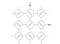
Figure 1: Orbital ordering by $\diagup=\psi_{1}=\frac{1}{\sqrt{2}}(\phi_{1}+\phi_{2})$, and $\diagdown=\psi_{2}=\frac{1}{\sqrt{2}}(\phi_{1}-\phi_{2})$, which have the occupation number $a+c$ in the $G(MB_{2g},0,0)$ state.

Note that this pattern has symmetries of $C_{2a},C_{2b},C_{2z},C_{2x}T(\mbox{\boldmath$e$}_{1})$ and $C_{2x}T(\mbox{\boldmath$e$}_{2})\in G(MB_{2g}0,0)$. From (71) we see that this state has alternating quadrupole moments, for $m$ such that $T(\mbox{\boldmath$m$})\in\mbox{\boldmath$L$}_{1}$, as follows

$$Q_{12}(\mbox{\boldmath$m$}) =4I_{2}c,\ Q_{12}(\mbox{\boldmath$m$}+\mbox{\boldmath$e$}_{j})=-4I_{2}c,\ j=1,2.$$ (169)

Finally we consider X point non magnetic state. As shown in Table 6, in cases of $G(X\gamma,0,\nu)_{1}$, isotropy subgroups contain $\mbox{\boldmath$L$}_{2}=\mbox{\boldmath$L$}(2\mbox{\boldmath$e$}_{1},\mbox{\boldmath$e$}_{2})$ and $S$. Thus from $\mbox{\boldmath$L$}_{2}=\mbox{\boldmath$L$}(2\mbox{\boldmath$e$}_{1},\mbox{\boldmath$e$}_{2})$ and $S$ invariance of $\mbox{\boldmath$R$}^{l\lambda}$, only $\mbox{\boldmath$R$}^{l0}\ (l=0,2)$ are non-zero. From (46), for $m$ such that $T(\mbox{\boldmath$m$})\in\mbox{\boldmath$L$}_{2}$, we have

$$\mbox{\boldmath$D$}(\mbox{\boldmath$m$}) =\mbox{\boldmath$D$}^{\uparrow\uparrow}(\mbox{\boldmath$m$})=\mbox{\boldmath$D$}^{\downarrow\downarrow}(\mbox{\boldmath$m$})=\mbox{\boldmath$R$}^{00}+\mbox{\boldmath$R$}^{20},$$

$$\mbox{\boldmath$D$}(\mbox{\boldmath$m$}+\mbox{\boldmath$e$}_{1}) =\mbox{\boldmath$D$}^{\uparrow\uparrow}(\mbox{\boldmath$m$}+\mbox{\boldmath$e$}_{1})=\mbox{\boldmath$D$}^{\downarrow\downarrow}(\mbox{\boldmath$m$}+\mbox{\boldmath$e$}_{1})=\mbox{\boldmath$R$}^{00}-\mbox{\boldmath$R$}^{20}.$$ (170)

In the cases of $G(X\gamma,0,\nu)_{2}$, isotropy subgroups contain $\mbox{\boldmath$L$}_{3}=\mbox{\boldmath$L$}(2\mbox{\boldmath$e$}_{1},2\mbox{\boldmath$e$}_{2})$ and $S$. Thus from $\mbox{\boldmath$L$}_{3}=\mbox{\boldmath$L$}(2\mbox{\boldmath$e$}_{1},2\mbox{\boldmath$e$}_{2})$ and $S$ invariance of $\mbox{\boldmath$R$}^{l\lambda}$, only $\mbox{\boldmath$R$}^{l0}\ (l=0,1,2,3)$ are non-zero. From (46), for $m$ such that $T(\mbox{\boldmath$m$})\in\mbox{\boldmath$L$}_{2}$, we have

$$\mbox{\boldmath$D$}(\mbox{\boldmath$m$}) =\mbox{\boldmath$D$}^{\uparrow\uparrow}(\mbox{\boldmath$m$})=\mbox{\boldmath$D$}^{\downarrow\downarrow}(\mbox{\boldmath$m$})=\mbox{\boldmath$R$}^{00}+\mbox{\boldmath$R$}^{10}+\mbox{\boldmath$R$}^{20}+\mbox{\boldmath$R$}^{30},$$

$$\mbox{\boldmath$D$}(\mbox{\boldmath$m$}+\mbox{\boldmath$e$}_{1}) =\mbox{\boldmath$D$}^{\uparrow\uparrow}(\mbox{\boldmath$m$}+\mbox{\boldmath$e$}_{1})=\mbox{\boldmath$D$}^{\downarrow\downarrow}(\mbox{\boldmath$m$}+\mbox{\boldmath$e$}_{1})=\mbox{\boldmath$R$}^{00}-\mbox{\boldmath$R$}^{10}-\mbox{\boldmath$R$}^{20}+\mbox{\boldmath$R$}^{30},$$

$$\mbox{\boldmath$D$}(\mbox{\boldmath$m$}+\mbox{\boldmath$e$}_{2}) =\mbox{\boldmath$D$}^{\uparrow\uparrow}(\mbox{\boldmath$m$}+\mbox{\boldmath$e$}_{2})=\mbox{\boldmath$D$}^{\downarrow\downarrow}(\mbox{\boldmath$m$}+\mbox{\boldmath$e$}_{2})=\mbox{\boldmath$R$}^{00}-\mbox{\boldmath$R$}^{10}+\mbox{\boldmath$R$}^{20}-\mbox{\boldmath$R$}^{30},$$

$$\mbox{\boldmath$D$}(\mbox{\boldmath$m$}+\mbox{\boldmath$e$}_{1}+\mbox{\boldmath$e$}_{2}) =\mbox{\boldmath$D$}^{\uparrow\uparrow}(\mbox{\boldmath$m$}+\mbox{\boldmath$e$}_{1}+\mbox{\boldmath$e$}_{2})=\mbox{\boldmath$D$}^{\downarrow\downarrow}(\mbox{\boldmath$m$}+\mbox{\boldmath$e$}_{1}+\mbox{\boldmath$e$}_{2})$$

$$=\mbox{\boldmath$R$}^{00}+\mbox{\boldmath$R$}^{10}-\mbox{\boldmath$R$}^{20}-\mbox{\boldmath$R$}^{{30}}.$$ (171)

We consider the $G(XB_{3g},0,1)_{2}$ state which breaks time reversal symmetry as an example.

Example 5.3.

$G(XB_{3},0,1)_{2}$ state.
Since

$$G(XB_{3g},0,1)_{2} =M_{z}T_{x}(\mbox{\boldmath$e$}_{2})T_{y}(\mbox{\boldmath$e$}_{1})\mbox{\boldmath$C$}_{2ah}\mbox{\boldmath$L$}_{3}\mbox{\boldmath$S$},$$ (172)

${\mbox{\boldmath$R$}^{l0}}\ (l=0,1,2,3)$ are invariant under $C_{2a},C_{2x}T(\mbox{\boldmath$e$}_{2}),C_{2y}T(\mbox{\boldmath$e$}_{1}),tC_{2z}$. Thus we obtain

$$\mbox{\boldmath$R$}^{00} =\left(\begin{array}[]{ccc}a&0&0\\ 0&a&0\\ 0&0&b\end{array}\right), \mbox{\boldmath$R$}^{10} =\left(\begin{array}[]{ccc}0&c&0\\ c&0&0\\ 0&0&0\end{array}\right),$$ (179)

$$\mbox{\boldmath$R$}^{20} =\left(\begin{array}[]{ccc}0&0&0\\ 0&0&id\\ 0&-id&0\end{array}\right), \mbox{\boldmath$R$}^{30} =\left(\begin{array}[]{ccc}0&0&-id\\ 0&0&0\\ id&0&0\end{array}\right),$$ (186)

where $a$, $b$, $c$ and $d$ are real numbers. Using (28) we obtain $H_{m}$ as

$$H_{m} =H_{\mathrm{K}}+\sum_{\mbox{\scriptsize\boldmath$k$}}\sum_{s}\{\alpha(a^{{\dagger}}_{1\mbox{\scriptsize\boldmath$k$}s}a_{1\mbox{\scriptsize\boldmath$k$}s}+a^{{\dagger}}_{2\mbox{\scriptsize\boldmath$k$}s}a_{2\mbox{\scriptsize\boldmath$k$}s})+\beta a^{{\dagger}}_{3\mbox{\scriptsize\boldmath$k$}s}a_{3\mbox{\scriptsize\boldmath$k$}s}$$

$$\ +\gamma(a^{{\dagger}}_{1(\mbox{\scriptsize\boldmath$k$}+\mbox{\scriptsize\boldmath$Q$}_{1})s}a_{2\mbox{\scriptsize\boldmath$k$}s}+a^{{\dagger}}_{2(\mbox{\scriptsize\boldmath$k$}+\mbox{\scriptsize\boldmath$Q$}_{1})s}a_{1\mbox{\scriptsize\boldmath$k$}s})$$

$$\ i\delta(a^{{\dagger}}_{2(\mbox{\scriptsize\boldmath$k$}+\mbox{\scriptsize\boldmath$Q$}_{2})s}a_{3\mbox{\scriptsize\boldmath$k$}s}-a^{{\dagger}}_{3(\mbox{\scriptsize\boldmath$k$}+\mbox{\scriptsize\boldmath$Q$}_{2})s}a_{2\mbox{\scriptsize\boldmath$k$}s}$$

$$\ -a^{{\dagger}}_{1(\mbox{\scriptsize\boldmath$k$}+\mbox{\scriptsize\boldmath$Q$}_{3})s}a_{3\mbox{\scriptsize\boldmath$k$}s}+a^{{\dagger}}_{3(\mbox{\scriptsize\boldmath$k$}+\mbox{\scriptsize\boldmath$Q$}_{3})s}a_{1\mbox{\scriptsize\boldmath$k$}s})\}$$

$$=H_{\mathrm{K}}+\alpha h(\Gamma A^{1}_{1g},0,0)_{1,0,1}+\beta h(\Gamma A^{2}_{1g},0,0)_{1,0,1}+\gamma h(MB_{2g},0,0)_{1,0,1}$$

$$\ \delta\{h(XB_{3g},0,1)_{1,0,1}+h(XB_{3g},0,1)_{2,0,1}\},$$ (187)

where $\alpha$, $\beta$, $\delta$ and $\gamma$ are determined by SCF conditions

$$\alpha =(U+2U^{\prime}-J)a+(2U^{\prime}-J)b,$$

$$\beta =2(2U^{\prime}-J)a+Ub,$$

$$\gamma =(2J+J^{\prime}-U^{\prime})c,$$

$$\delta =(2J-J^{\prime}-U^{\prime})d.$$ (188)

The fifth term of (187) is the primary part which leads to the transition to the $G(XB_{3g},0,1)_{2}$ state. The fourth term of (187) is the secondary part induced by the transition.

The HF energy is written as

$$E_{\mathrm{HF}} =\langle H_{\mathrm{K}}\rangle^{\prime}+\dfrac{N}{2}\{2(U+2U^{\prime}-J)a^{2}+Ub^{2}+4(2U^{\prime}-J)ab\}$$

$$\ \ +\dfrac{N}{2}\{2(2J+J^{\prime}-U^{\prime})c^{2}+4(2J-U^{\prime}-J^{\prime})d^{2}\}.$$ (189)

From (171) we obtain, for $m$ such that $T(\mbox{\boldmath$m$})\in\mbox{\boldmath$L$}_{3}$,

$$\mbox{\boldmath$D$}(\mbox{\boldmath$m$}) =\left(\begin{array}[]{ccc}a&c&-id\\ c&a&id\\ id&-id&b\end{array}\right), \mbox{\boldmath$D$}(\mbox{\boldmath$m$}+\mbox{\boldmath$e$}_{2}) =\left(\begin{array}[]{ccc}a&-c&id\\ -c&a&id\\ -id&-id&b\end{array}\right),$$ (196)

$$\mbox{\boldmath$D$}(\mbox{\boldmath$m$}+\mbox{\boldmath$e$}_{1}) =\left(\begin{array}[]{ccc}a&-c&-id\\ -c&a&-id\\ id&id&b\end{array}\right), \mbox{\boldmath$D$}(\mbox{\boldmath$m$}+\mbox{\boldmath$e$}_{1}+\mbox{\boldmath$e$}_{2}) =\left(\begin{array}[]{ccc}a&c&id\\ c&a&-id\\ -id&id&b\end{array}\right).$$ (203)

Table 8: Occupied atomic orbitals and their occupation numbers for $G(XB_{3g},0,1)_{2}$ state

site	spin	atomic orbital	occupation number
$m$	$\uparrow\downarrow$	$\psi_{1}=\frac{1}{\sqrt{2}}\mathrm{sgn}(d)u\phi_{1}-\frac{1}{\sqrt{2}}\mathrm{sgn}(d)u\phi_{2}+iw\phi_{3}$	$\lambda_{1}$
$m$	$\uparrow\downarrow$	$\psi_{2}=-\frac{1}{\sqrt{2}}\mathrm{sgn}(d)w\phi_{1}+\frac{1}{\sqrt{2}}\mathrm{sgn}(d)w\phi_{2}+iu\phi_{3}$	$\lambda_{2}$
$m$	$\uparrow\downarrow$	$\psi_{3}=\frac{1}{\sqrt{2}}(\phi_{1}+\phi_{2})$	$\lambda_{3}$
$\mbox{\boldmath$m$}+\mbox{\boldmath$e$}_{1}$	$\uparrow\downarrow$	$\psi_{1}=-\frac{1}{\sqrt{2}}\mathrm{sgn}(d)u\phi_{1}-\frac{1}{\sqrt{2}}\mathrm{sgn}(d)u\phi_{2}-iw\phi_{3}$	$\lambda_{1}$
$\mbox{\boldmath$m$}+\mbox{\boldmath$e$}_{1}$	$\uparrow\downarrow$	$\psi_{2}=-\frac{1}{\sqrt{2}}\mathrm{sgn}(d)w\phi_{1}-\frac{1}{\sqrt{2}}\mathrm{sgn}(d)w\phi_{2}+iu\phi_{3}$	$\lambda_{2}$
$\mbox{\boldmath$m$}+\mbox{\boldmath$e$}_{1}$	$\uparrow\downarrow$	$\psi_{3}=\frac{1}{\sqrt{2}}(\phi_{1}-\phi_{2})$ $\lambda_{3}$
$\mbox{\boldmath$m$}+\mbox{\boldmath$e$}_{2}$	$\uparrow\downarrow$	$\psi_{1}=\frac{1}{\sqrt{2}}\mathrm{sgn}(d)u\phi_{1}+\frac{1}{\sqrt{2}}\mathrm{sgn}(d)u\phi_{2}-iw\phi_{3}$	$\lambda_{1}$
$\mbox{\boldmath$m$}+\mbox{\boldmath$e$}_{2}$	$\uparrow\downarrow$	$\psi_{2}=\frac{1}{\sqrt{2}}\mathrm{sgn}(d)w\phi_{1}+\frac{1}{\sqrt{2}}\mathrm{sgn}(d)w\phi_{2}+iu\phi_{3}$	$\lambda_{2}$
$\mbox{\boldmath$m$}+\mbox{\boldmath$e$}_{2}$	$\uparrow\downarrow$	$\psi_{3}=\frac{1}{\sqrt{2}}(\phi_{1}-\phi_{2})$	$\lambda_{3}$
$\mbox{\boldmath$m$}+\mbox{\boldmath$e$}_{1}+\mbox{\boldmath$e$}_{2}$	$\uparrow\downarrow$	$\psi_{1}=-\frac{1}{\sqrt{2}}\mathrm{sgn}(d)u\phi_{1}+\frac{1}{\sqrt{2}}\mathrm{sgn}(d)u\phi_{2}+iw\phi_{3}$	$\lambda_{1}$
$\mbox{\boldmath$m$}+\mbox{\boldmath$e$}_{1}+\mbox{\boldmath$e$}_{2}$	$\uparrow\downarrow$	$\psi_{2}=\frac{1}{\sqrt{2}}\mathrm{sgn}(d)w\phi_{1}-\frac{1}{\sqrt{2}}\mathrm{sgn}(d)w\phi_{2}+iu\phi_{3}$	$\lambda_{2}$
$\mbox{\boldmath$m$}+\mbox{\boldmath$e$}_{1}+\mbox{\boldmath$e$}_{2}$	$\uparrow\downarrow$	$\psi_{3}=\frac{1}{\sqrt{2}}(\phi_{1}+\phi_{2})$	$\lambda_{3}$
$T(\mbox{\boldmath$m$})\in\mbox{\boldmath$L$}_{3}=(2\mbox{\boldmath$e$}_{1},2\mbox{\boldmath$e$}_{2})$
$a=R^{00}_{11}=R^{00}_{22},\ b=R^{00}_{33},\ c=R^{10}_{12}=R^{10}_{21},\ id=R^{20}_{23}=-R^{20}_{32}=-R^{30}_{13}=R^{30}_{31}$
$u=\frac{1}{\sqrt{2}}(1+\frac{a-b-c}{\sqrt{{(a-b-c)^{2}+8d^{2}}}})^{\frac{1}{2}},w=\frac{1}{\sqrt{2}}(1-\frac{a-b-c}{\sqrt{{(a-b-c)^{2}+8d^{2}}}})^{\frac{1}{2}}$
$\lambda_{1}=\frac{a+b-c+\sqrt{(a-b-c)^{2}+8d^{2}}}{2},\lambda_{2}=\frac{a+b-c-\sqrt{(a-b-c)^{2}+8d^{2}}}{2},\lambda_{3}=a+c$

Figure 2: The ordering pattern for quadrupole moments: $Q_{12}$ and orbital angular momenta:                  $\mbox{\boldmath$l$}=(l_{1},l_{2})$ in the $G(XB_{3g}0,1)_{2}$ state. The ovals and arrows represent $Q_{12}$ and orbital angular momentum $l$, respectively.

Diagonalizing $\mbox{\boldmath$D$}(\mbox{\boldmath$m$}),\mbox{\boldmath$D$}(\mbox{\boldmath$m$}+\mbox{\boldmath$e$}_{1}),\mbox{\boldmath$D$}(\mbox{\boldmath$m$}+\mbox{\boldmath$e$}_{2}),\mbox{\boldmath$D$}(\mbox{\boldmath$m$}+\mbox{\boldmath$e$}_{1}+\mbox{\boldmath$e$}_{2})$, we obtain occupied atomic orbitals and their occupation numbers at the sites $\mbox{\boldmath$m$},\mbox{\boldmath$m$}+\mbox{\boldmath$e$}_{1},\mbox{\boldmath$m$}+\mbox{\boldmath$e$}_{2},\mbox{\boldmath$m$}+\mbox{\boldmath$e$}_{1}+\mbox{\boldmath$e$}_{2}$ for the $G(XB_{3g},0,1)_{2}$ state as shown in Table 8. Note that occupied atomic orbitals have complex coefficients.

From (71), we see that this state has the following orbital angular momentum(the primary LOP) and quadrupole moment(the secondary LOP). For $m$ such that $T(\mbox{\boldmath$m$})\in\mbox{\boldmath$L$}_{3}$, we obtain

$$l_{1}(\mbox{\boldmath$m$}) =4d,\ \ \ \ l_{2}(\mbox{\boldmath$m$})=4d,$$

$$l_{1}(\mbox{\boldmath$m$}+\mbox{\boldmath$e$}_{1}) =-4d,\ \ \ l_{2}(\mbox{\boldmath$m$}+\mbox{\boldmath$e$}_{1})=4d,$$

$$l_{1}(\mbox{\boldmath$m$}+\mbox{\boldmath$e$}_{2}) =4d,\ \ \ \ l_{2}(\mbox{\boldmath$m$}+\mbox{\boldmath$e$}_{2})=-4d,$$

$$l_{1}(\mbox{\boldmath$m$}+\mbox{\boldmath$e$}_{1}+\mbox{\boldmath$e$}_{2}) =-4d,\ \ \ l_{2}(\mbox{\boldmath$m$}+\mbox{\boldmath$e$}_{1}+\mbox{\boldmath$e$}_{2})=-4d$$

$$Q_{12}(\mbox{\boldmath$m$}) =4I_{2}c,\hskip 19.91692ptQ_{12}(\mbox{\boldmath$m$}+\mbox{\boldmath$e$}_{1})=-4I_{2}c,$$

$$Q_{12}(\mbox{\boldmath$m$}+\mbox{\boldmath$e$}_{2}) =-4I_{2}c,\ \ Q_{12}(\mbox{\boldmath$m$}+\mbox{\boldmath$e$}_{1}+\mbox{\boldmath$e$}_{2})=4I_{2}c$$ (204)

The ordering pattern of $Q_{12}$ and $\mbox{\boldmath$l$}=(l_{1},l_{2})$ for the $G(XB_{3g},0,1)_{3}$ state is shown in Fig. 2. Note that the onset of quadrupole moment $Q_{12}$ is induced by the transition to the $G(XB_{3g},0,1)_{2}$ with the orbital angular momentum.

By a similar manner to the case of $G(XB_{3g},0,1)_{2}$, we can see that all states having isotropy subgroups such as $G(\Lambda,0,1)$ or $G(\Lambda,0,1)_{j}~{}(j=1,2)$, which break the time reversal symmetry, have complex occupied orbitals and orbital angular momentum as LOP.

6 Symmetry classes of magnetic orbital ordered states

In order to list magnetic orbital ordered states with ordering vectors $\mbox{\boldmath$Q$}_{l}\ (l=0,1,2,3)$, bifurcating from the normal state, we present the axial isotropy subgroups of the R-reps $\check{G}_{0}^{(\Gamma j,1,\nu)},\check{G}_{0}^{(Mj,1,\nu)}$ and $\check{G}_{0}^{(X\gamma,1,\nu)}$. The axial isotropy subgroups of R-reps $\check{G}_{0}^{(\Gamma j,1,\nu)}$ and $\check{G}_{0}^{(Mj,1,\nu)}$ are listed in Table 9.

Table 9: Axial isotropy subgroup and its Fixed point subspace of $\check{G}_{0}^{(\Gamma j,1,\nu)}$ and $\check{G}_{0}^{(Mj,1,\nu)}$

R-rep	axial isotropy subgroup	Fixed point subspace
$\check{G}_{0}^{(\Gamma A_{1g},1,1)}$	$G(\Gamma A_{1g},1,1)=M(\mbox{\boldmath$e$}_{2})\mbox{\boldmath$D$}_{4h}\mbox{\boldmath$L$}_{0}\mbox{\boldmath$A$}(\mbox{\boldmath$e$}_{3})$	$\{h_{1,1,1}\}_{\mathrm{R}}$
$\check{G}_{0}^{(\Gamma A_{2g},1,0)}$	$G(\Gamma A_{2g},1,0)=\mbox{\boldmath$D$}_{4h}(E,u_{2x})\mbox{\boldmath$L$}_{0}\mbox{\boldmath$A$}(\mbox{\boldmath$e$}_{3})\bf{R}$	$\{h_{1,3,1}\}_{\mathrm{R}}$
$\check{G}_{0}^{(\Gamma B_{1g},1,1)}$	$G(\Gamma B_{1g},1,1)=M(\mbox{\boldmath$e$}_{2})\mbox{\boldmath$D$}_{4h}(u_{2x},E)\mbox{\boldmath$L$}_{0}\mbox{\boldmath$A$}(\mbox{\boldmath$e$}_{3})$	$\{h_{1,3,1}\}_{\mathrm{R}}$
$\check{G}_{0}^{(\Gamma B_{2g},1,1)}$	$G(\Gamma B_{2g},1,1)=M(\mbox{\boldmath$e$}_{2})\mbox{\boldmath$D$}_{4h}(u_{2x},u_{2x})\mbox{\boldmath$L$}_{0}\mbox{\boldmath$A$}(\mbox{\boldmath$e$}_{3})$	$\{h_{1,3,1}\}_{\mathrm{R}}$
$\check{G}_{0}^{(\Gamma E_{g},1,1)}$	$G(\Gamma E_{g},1,1)_{1}=M(\mbox{\boldmath$e$}_{2})\mbox{\boldmath$D$}_{2h}(u_{2x},E)\mbox{\boldmath$L$}_{0}\mbox{\boldmath$A$}(\mbox{\boldmath$e$}_{3})$	$\{h_{1,3,1}\}_{\mathrm{R}}$
	$G(\Gamma E_{g},1,1)_{2}=M(\mbox{\boldmath$e$}_{2})\mbox{\boldmath$D$}_{2ah}(u_{2x},E)\mbox{\boldmath$L$}_{0}\mbox{\boldmath$A$}(\mbox{\boldmath$e$}_{3})$	$\{h_{1,3,1}+h_{2,3,1}\}_{\mathrm{R}}$
	$G(\Gamma E_{g},1,1)_{3}=M(\mbox{\boldmath$e$}_{3})\mbox{\boldmath$D$}_{4h}(u_{4z}^{+},u_{2x})\mbox{\boldmath$L$}_{0}$	$\{h_{1,1,1}+h_{2,2,1}\}_{\mathrm{R}}$
$\check{G}_{0}^{(\Gamma E_{g},1,0)}$	$G(\Gamma E_{g},1,0)_{1}=\mbox{\boldmath$D$}_{2h}(u_{2x},E)\mbox{\boldmath$L$}_{0}\mbox{\boldmath$A$}(\mbox{\boldmath$e$}_{3})\bf{R}$	$\{h_{1,3,1}\}_{\mathrm{R}}$
	$G(\Gamma E_{g},1,0)_{2}=\mbox{\boldmath$D$}_{2ah}(u_{2x},E)\mbox{\boldmath$L$}_{0}\mbox{\boldmath$A$}(\mbox{\boldmath$e$}_{3})\bf{R}$	$\{h_{1,3,1}+h_{2,3,1}\}_{\mathrm{R}}$
	$G(\Gamma E_{g},1,0)_{3}=\mbox{\boldmath$D$}_{4h}(u_{4z}^{+},u_{2x})\mbox{\boldmath$L$}_{0}\bf{R}$	$\{h_{1,3,1}+h_{2,2,1}\}_{\mathrm{R}}$
$\check{G}_{0}^{(MA_{1g},1,1)}$	$G(MA_{1g},1,1)=M(\mbox{\boldmath$e$}_{2})T^{x}(\mbox{\boldmath$e$}_{1})\mbox{\boldmath$D$}_{4h}\mbox{\boldmath$L$}_{1}\mbox{\boldmath$A$}(\mbox{\boldmath$e$}_{3})$	$\{h_{1,1,1}\}_{\mathrm{R}}$
$\check{G}_{0}^{(MA_{2g},1,0)}$	$G(MA_{2g},1,0)=T_{x}(\mbox{\boldmath$e$}_{1})T^{x}(\mbox{\boldmath$e$}_{1})\mbox{\boldmath$D$}_{4h}(E,u_{2x})\mbox{\boldmath$L$}_{1}\mbox{\boldmath$A$}(\mbox{\boldmath$e$}_{3})\bf{R}$	$\{h_{1,3,1}\}_{\mathrm{R}}$
$\check{G}_{0}^{(MB_{1g},1,1)}$	$G(MB_{1g},1,1)=M(\mbox{\boldmath$e$}_{2})T^{x}(\mbox{\boldmath$e$}_{1})T_{a}(\mbox{\boldmath$e$}_{1})\mbox{\boldmath$D$}_{4h}(u_{2x},E)\mbox{\boldmath$L$}_{1}\mbox{\boldmath$A$}(\mbox{\boldmath$e$}_{3})$	$\{h_{1,3,1}\}_{\mathrm{R}}$
$\check{G}_{0}^{(MB_{2g},1,1)}$	$G(MB_{2g},1,1)=M(\mbox{\boldmath$e$}_{2})T^{x}(\mbox{\boldmath$e$}_{1})T_{x}(\mbox{\boldmath$e$}_{1})\mbox{\boldmath$D$}_{4h}(u_{2x},u_{2x})\mbox{\boldmath$L$}_{1}\mbox{\boldmath$A$}(\mbox{\boldmath$e$}_{3})$	$\{h_{1,3,1}\}_{\mathrm{R}}$
$\check{G}_{0}^{(ME_{g},1,1)}$	$G(ME_{g},1,1)_{1}=M(\mbox{\boldmath$e$}_{2})T^{x}(\mbox{\boldmath$e$}_{1})T_{y}(\mbox{\boldmath$e$}_{1})\mbox{\boldmath$D$}_{2h}(u_{2x},E)\mbox{\boldmath$L$}_{1}\mbox{\boldmath$A$}(\mbox{\boldmath$e$}_{3})$	$\{h_{1,3,1}\}_{\mathrm{R}}$
	$G(ME_{g},1,1)_{2}=M(\mbox{\boldmath$e$}_{2})T^{x}(\mbox{\boldmath$e$}_{1})T_{b}(\mbox{\boldmath$e$}_{1})\mbox{\boldmath$D$}_{2ah}(u_{2x},E)\mbox{\boldmath$L$}_{1}\mbox{\boldmath$A$}(\mbox{\boldmath$e$}_{3})$	$\{h_{1,3,1}+h_{2,3,1}\}_{\mathrm{R}}$
	$G(ME_{g},1,1)_{3}=M(\mbox{\boldmath$e$}_{3})T_{z}(\mbox{\boldmath$e$}_{1})\mbox{\boldmath$D$}_{4h}(u_{4z}^{+},u_{2x})\mbox{\boldmath$L$}_{1}$	$\{h_{1,1,1}+h_{2,2,1}\}_{\mathrm{R}}$
$\check{G}_{0}^{(ME_{g},1,0)}$	$G(ME_{g},1,0)_{1}=T^{x}(\mbox{\boldmath$e$}_{1})T_{y}(\mbox{\boldmath$e$}_{1})\mbox{\boldmath$D$}_{2h}(u_{2x},E)\mbox{\boldmath$L$}_{1}\mbox{\boldmath$A$}(\mbox{\boldmath$e$}_{3})\bf{R}$	$\{h_{1,3,1}\}_{\mathrm{R}}$
	$G(ME_{g},1,0)_{2}=T^{x}(\mbox{\boldmath$e$}_{1})T_{y}(\mbox{\boldmath$e$}_{1})\mbox{\boldmath$D$}_{2ah}(u_{2x},E)\mbox{\boldmath$L$}_{1}\mbox{\boldmath$A$}(\mbox{\boldmath$e$}_{3})\bf{R}$	$\{h_{1,3,1}+h_{2,3,1}\}_{\mathrm{R}}$
	$G(ME_{g},1,0)_{3}=T^{z}(\mbox{\boldmath$e$}_{1})T_{z}(\mbox{\boldmath$e$}_{1})\mbox{\boldmath$D$}_{4h}(u_{4z}^{+},u_{2x})\mbox{\boldmath$L$}_{1}\bf{R}$	$\{h_{1,3,1}+h_{2,2,1}\}_{\mathrm{R}}$
$\mbox{\boldmath$L$}_{0}=\mbox{\boldmath$L$}(\mbox{\boldmath$e$}_{1},\mbox{\boldmath$e$}_{2}),\ \mbox{\boldmath$L$}_{1}=\mbox{\boldmath$L$}(\mbox{\boldmath$e$}_{1}+\mbox{\boldmath$e$}_{2},\mbox{\boldmath$e$}_{2}-\mbox{\boldmath$e$}_{1})$
$u_{2i}=u(\mbox{\boldmath$e$}_{i},\pi)\in\mbox{\boldmath$S$},\ M(\mbox{\boldmath$e$}_{i})=\{E,tu_{2i}\}$
$\mbox{\boldmath$A$}(\mbox{\boldmath$e$}_{i})=\{u(\mbox{\boldmath$e$}_{3},\theta)\mid 0\leq\theta\leq 2\pi\}$
$\mbox{\boldmath$D$}_{4h}(\alpha,\beta)=\{(E,C_{4z}^{+}\alpha,C_{2z}\alpha^{2},C_{4z}^{-}\alpha^{-})+C_{2x}\beta(E,C_{4z}^{+}\alpha,C_{2z}\alpha^{2},C_{4z}^{-}\alpha^{-})\}\times\mbox{\boldmath$C$}_{I}$
$\mbox{\boldmath$D$}_{2h}(\alpha,\beta)=\{(E,C_{2z}\alpha)+C_{2x}\beta(E,C_{2z}\alpha)\}\times\mbox{\boldmath$C$}_{I}$
$\mbox{\boldmath$D$}_{2ah}(\alpha,\beta)=\{(E,C_{2z}\alpha)+C_{2a}\beta(E,C_{2z}\alpha)\}\times\mbox{\boldmath$C$}_{I}$
$T^{i}(\mbox{\boldmath$e$}_{m})=\{E,u_{2i}T(\mbox{\boldmath$e$}_{m})\}$
$T_{i}(\mbox{\boldmath$e$}_{m})=\{E,C_{2i}T(\mbox{\boldmath$e$}_{m})\}$

Those of $\check{G}_{0}^{(Xj,1,\nu)}$ are listed in Table 10.

Table 10: Axial isotropy subgroup and its Fixed point subspace of $\check{G}_{0}^{(Xj,1,\nu)}$

R-rep	axial isotropy subgroup	Fixed point subspace
$\check{G}_{0}^{(XA_{1g},1,1)}$	$G(XA_{1g},1,1)_{1}=M(\mbox{\boldmath$e$}_{2})T^{x}(\mbox{\boldmath$e$}_{1})\mbox{\boldmath$D$}_{2h}\mbox{\boldmath$L$}_{2}\mbox{\boldmath$A$}(\mbox{\boldmath$e$}_{3})$	$\{h_{1,3,1}\}_{\mathrm{R}}$
	$G(XA_{1g},1,1)_{2}=M(\mbox{\boldmath$e$}_{2})T^{x}(\mbox{\boldmath$e$}_{1}+\mbox{\boldmath$e$}_{2})\mbox{\boldmath$D$}_{4h}\mbox{\boldmath$L$}_{3}\mbox{\boldmath$A$}(\mbox{\boldmath$e$}_{3})$	$\{h_{1,3,1}+h_{2,3,1}\}_{\mathrm{R}}$
	$G(XA_{1g},1,1)_{3}=M(\mbox{\boldmath$e$}_{3})T^{x}(\mbox{\boldmath$e$}_{2})T^{y}(\mbox{\boldmath$e$}_{1})\mbox{\boldmath$D$}_{4h}(u_{2a},E)\mbox{\boldmath$L$}_{3}$	$\{h_{1,1,1}+h_{2,2,1}\}_{\mathrm{R}}$
$\check{G}_{0}^{(XB_{1g},1,1)}$	$G(XB_{1g},1,1)_{1}=M(\mbox{\boldmath$e$}_{2})T^{x}(\mbox{\boldmath$e$}_{1})\mbox{\boldmath$D$}_{2h}(E,u_{2x})\mbox{\boldmath$L$}_{2}\mbox{\boldmath$A$}(\mbox{\boldmath$e$}_{3})$	$\{h_{1,3,1}\}_{\mathrm{R}}$
	$G(XB_{1g},1,1)_{2}=M(\mbox{\boldmath$e$}_{2})T^{x}(\mbox{\boldmath$e$}_{1}+\mbox{\boldmath$e$}_{2})\mbox{\boldmath$D$}_{4h}(u_{2x},u_{2x})\mbox{\boldmath$L$}_{3}\mbox{\boldmath$A$}(\mbox{\boldmath$e$}_{3})$	$\{h_{1,3,1}+h_{2,3,1}\}_{\mathrm{R}}$
	$G(XB_{1g},1,1)_{3}=M(\mbox{\boldmath$e$}_{3})T^{x}(\mbox{\boldmath$e$}_{2})T^{y}(\mbox{\boldmath$e$}_{1})\mbox{\boldmath$D$}_{4h}(u_{2b},u_{2x})\mbox{\boldmath$L$}_{3}$	$\{h_{1,1,1}+h_{2,2,1}\}_{\mathrm{R}}$
$\check{G}_{0}^{(XB_{2g},1,1)}$	$G(XB_{2g},1,1)_{1}=M(\mbox{\boldmath$e$}_{2})T^{x}(\mbox{\boldmath$e$}_{1})\mbox{\boldmath$D$}_{2h}(u_{2x},u_{2x})\mbox{\boldmath$L$}_{2}\mbox{\boldmath$A$}(\mbox{\boldmath$e$}_{3})$	$\{h_{1,3,1}\}_{\mathrm{R}}$
	$G(XB_{2g},1,1)_{2}=M(\mbox{\boldmath$e$}_{2})T_{x}(\mbox{\boldmath$e$}_{1})T_{y}(\mbox{\boldmath$e$}_{2})\mbox{\boldmath$D$}_{2ah}(u_{2x},E)\mbox{\boldmath$L$}_{3}\mbox{\boldmath$A$}(\mbox{\boldmath$e$}_{3})$	$\{h_{1,3,1}+h_{2,3,1}\}_{\mathrm{R}}$
	$G(XB_{2g},1,1)_{3}=M(\mbox{\boldmath$e$}_{3})T_{x}(\mbox{\boldmath$e$}_{1})T_{y}(\mbox{\boldmath$e$}_{2})\mbox{\boldmath$D$}_{4h}(u_{4z}^{+},u_{2x})\mbox{\boldmath$L$}_{3}$	$\{h_{1,1,1}+h_{2,2,1}\}_{\mathrm{R}}$
$\check{G}_{0}^{(XB_{3g},1,1)}$	$G(XB_{3g},1,1)_{1}=M(\mbox{\boldmath$e$}_{2})T_{y}(\mbox{\boldmath$e$}_{1})\mbox{\boldmath$D$}_{2h}(u_{2x},E)\mbox{\boldmath$L$}_{2}\mbox{\boldmath$A$}(\mbox{\boldmath$e$}_{3})$	$\{h_{1,3,1}\}_{\mathrm{R}}$
	$G(XB_{3g},1,1)_{2}=M(\mbox{\boldmath$e$}_{2})T_{x}(\mbox{\boldmath$e$}_{2})T_{y}(\mbox{\boldmath$e$}_{1})\mbox{\boldmath$D$}_{2ah}(u_{2x},E)\mbox{\boldmath$L$}_{3}\mbox{\boldmath$A$}(\mbox{\boldmath$e$}_{3})$	$\{h_{1,3,1}+h_{2,3,1}\}_{\mathrm{R}}$
	$G(XB_{3g},1,1)_{3}=M(\mbox{\boldmath$e$}_{3})T_{x}(\mbox{\boldmath$e$}_{2})T_{y}(\mbox{\boldmath$e$}_{1})\mbox{\boldmath$D$}_{4h}(u_{4z}^{+},u_{2x})\mbox{\boldmath$L$}_{3}$	$\{h_{1,1,1}+h_{2,2,1}\}_{\mathrm{R}}$
$\check{G}_{0}^{(XB_{1g},1,0)}$	$G(XB_{1g},1,0)_{1}=T^{x}(\mbox{\boldmath$e$}_{1})\mbox{\boldmath$D$}_{2h}(E,u_{2x})\mbox{\boldmath$L$}_{2}\mbox{\boldmath$A$}(\mbox{\boldmath$e$}_{3})\bf{R}$	$\{h_{1,3,1}\}_{\mathrm{R}}$
	$G(XB_{1g},1,0)_{2}=T^{x}(\mbox{\boldmath$e$}_{1}+\mbox{\boldmath$e$}_{2})\mbox{\boldmath$D$}_{4h}(u_{2x},u_{2x})\mbox{\boldmath$L$}_{3}\mbox{\boldmath$A$}(\mbox{\boldmath$e$}_{3})\bf{R}$	$\{h_{1,3,1}+h_{2,3,1}\}_{\mathrm{R}}$
	$G(XB_{1g},1,0)_{3}=T^{x}(\mbox{\boldmath$e$}_{2})T^{y}(\mbox{\boldmath$e$}_{1})\mbox{\boldmath$D$}_{4h}(u_{2b},u_{2x})\mbox{\boldmath$L$}_{3}\bf{R}$	$\{h_{1,1,1}+h_{2,2,1}\}_{\mathrm{R}}$
$\check{G}_{0}^{(XB_{2g},1,0)}$	$G(XB_{2g},1,0)_{1}=T^{x}(\mbox{\boldmath$e$}_{1})\mbox{\boldmath$D$}_{2h}(u_{2x},u_{2x})\mbox{\boldmath$L$}_{2}\mbox{\boldmath$A$}(\mbox{\boldmath$e$}_{3})\bf{R}$	$\{h_{1,3,1}\}_{\mathrm{R}}$
	$G(XB_{2g},1,0)_{2}=T_{x}(\mbox{\boldmath$e$}_{1})T_{y}(\mbox{\boldmath$e$}_{2})\mbox{\boldmath$D$}_{2ah}(u_{2x},E)\mbox{\boldmath$L$}_{3}\mbox{\boldmath$A$}(\mbox{\boldmath$e$}_{3})\bf{R}$	$\{h_{1,3,1}+h_{2,3,1}\}_{\mathrm{R}}$
	$G(XB_{2g},1,0)_{3}=T_{x}(\mbox{\boldmath$e$}_{1})T_{y}(\mbox{\boldmath$e$}_{2})\mbox{\boldmath$D$}_{4h}(u_{4z}^{+},u_{2x})\mbox{\boldmath$L$}_{3}\bf{R}$	$\{h_{1,1,1}+h_{2,2,1}\}_{\mathrm{R}}$
$\check{G}_{0}^{(XB_{3g},1,0)}$	$G(XB_{3g},1,0)_{1}=T_{y}(\mbox{\boldmath$e$}_{1})\mbox{\boldmath$D$}_{2h}(u_{2x},E)\mbox{\boldmath$L$}_{2}\mbox{\boldmath$A$}(\mbox{\boldmath$e$}_{3})\bf{R}$	$\{h_{1,3,1}\}_{\mathrm{R}}$
	$G(XB_{3g},1,0)_{2}=T_{x}(\mbox{\boldmath$e$}_{2})T_{y}(\mbox{\boldmath$e$}_{1})\mbox{\boldmath$D$}_{2ah}(u_{2x},E)\mbox{\boldmath$L$}_{3}\mbox{\boldmath$A$}(\mbox{\boldmath$e$}_{3})\bf{R}$	$\{h_{1,3,1}+h_{2,3,1}\}_{\mathrm{R}}$
	$G(XB_{2g},1,0)_{3}=T_{x}(\mbox{\boldmath$e$}_{2})T_{y}(\mbox{\boldmath$e$}_{1})\mbox{\boldmath$D$}_{4h}(u_{4z}^{+},u_{2x})\mbox{\boldmath$L$}_{3}\bf{R}$	$\{h_{1,1,1}+h_{2,2,1}\}_{\mathrm{R}}$
$\mbox{\boldmath$L$}_{2}=\mbox{\boldmath$L$}(2\mbox{\boldmath$e$}_{1},\mbox{\boldmath$e$}_{2}),\ \mbox{\boldmath$L$}_{3}=\mbox{\boldmath$L$}(2\mbox{\boldmath$e$}_{1},2\mbox{\boldmath$e$}_{2})$
$u_{2i}=u(\mbox{\boldmath$e$}_{i},\pi),u_{2a}=u(\mbox{\boldmath$e$}_{1}+\mbox{\boldmath$e$}_{2},\pi),u_{2b}=u(-\mbox{\boldmath$e$}_{1}+\mbox{\boldmath$e$}_{2},\pi)\in\mbox{\boldmath$S$}$
$M(\mbox{\boldmath$e$}_{i})=\{E,tu_{2i}\},\ T^{i}(\mbox{\boldmath$e$}_{m})=\{E,u_{2i}T(\mbox{\boldmath$e$}_{m})\},\ T_{i}(\mbox{\boldmath$e$}_{m})=\{E,C_{2i}T(\mbox{\boldmath$e$}_{m})\}$
$\mbox{\boldmath$D$}_{2h}(\alpha,\beta)=\{(E,C_{2z}\alpha)+C_{2x}\beta(E,C_{2z}\alpha)\}\times\mbox{\boldmath$C$}_{I}$
$\mbox{\boldmath$D$}_{2ah}(\alpha,\beta)=\{(E,C_{2z}\alpha)+C_{2a}\beta(E,C_{2z}\alpha)\}\times\mbox{\boldmath$C$}_{I}$
$\mbox{\boldmath$D$}_{4h}(\alpha,\beta)=\{(E,C_{4z}^{+}\alpha,C_{2z}\alpha^{2},C_{4z}^{-}\alpha^{-1})+C_{2x}\beta(E,C_{4z}^{+}\alpha,C_{2z}\alpha^{2},C_{4z}^{-}\alpha^{-1})\}\times\mbox{\boldmath$C$}_{I}$

Spin magnetic states are classified into two groups: collinear and non-collinear magnetic states. The collinear magnetic state has the isotropy subgroup containing the subgroup $\mbox{\boldmath$A$}(\mbox{\boldmath$e$}_{3})$: the spin rotation around $z$ axis. The isotropy subgroup of the non-collinear magnetic state does not contain $\mbox{\boldmath$A$}(\mbox{\boldmath$e$}_{3})$.

Non-collinear magnetic states are derived from the R-reps: $G_{0}^{(\Lambda E_{g},1,1)}$, $G_{0}^{(\Lambda E_{g},1,0)}$, $G_{0}^{(XA_{1g},1,1)}$, $G_{0}^{(XB_{jg},1,1)}$ and $G_{0}^{(XB_{jg},1,0)}$ where $\Lambda=\Gamma,M$ and $j=1,2,3$. The corresponding non-collinear magnetic states are $G(\Gamma E_{g},1,1)_{3},G(\Gamma E_{g},1,0)_{3},$
$G(ME_{g},1,1)_{3},G(ME_{g},1,0)_{3},G(XA_{g},1,1)_{3},G(XB_{ig},1,1)_{3}$ and $G(XB_{ig},1,0)_{3}\ (i=1,2,3)$. All states in Table 9 and 10 except these eleven states are collinear magnetic states. We consider collinear and non-collinear magnetic states seperately.

6.1 Collinear magnetic state

All axial isotropy subgroups of collinear magnetic states contain $A(\mbox{\boldmath$e$}_{3})$, then $\mbox{\boldmath$R$}^{l1}=\mbox{\boldmath$R$}^{l2}=0$ for $l=0,1,2,3$. Thus in these cases we obtain from (46)

$$\mbox{\boldmath$D$}^{\uparrow\downarrow}(\mbox{\boldmath$m$}) =\mbox{\boldmath$D$}^{\downarrow\uparrow}(\mbox{\boldmath$m$})=0.$$ (205)

We consider two examples.

Example 6.1.

$G(\Gamma A_{1g},1,1)$ state.
In this case, the isotropy subgroup $G(H_{m})$ of $H_{m}$ is

$$G(\Gamma A_{1g},1,1) =M(\mbox{\boldmath$e$}_{2})\mbox{\boldmath$D$}_{4h}\mbox{\boldmath$L$}_{0}\mbox{\boldmath$A$}(\mbox{\boldmath$e$}_{3}).$$ (206)

From $\mbox{\boldmath$L$}_{0}$ invariance of $\mbox{\boldmath$R$}^{l\lambda}$ we can see that only $\mbox{\boldmath$R$}^{00}$ and $\mbox{\boldmath$R$}^{03}$ are non-zero.
From $C_{2x},C_{2z},C_{2a}(\in\mbox{\boldmath$D$}_{4h})$ invariance of $\mbox{\boldmath$R$}^{00}$ and $\mbox{\boldmath$R$}^{03}$, we obtain

$$\mbox{\boldmath$R$}^{00} =\left(\begin{array}[]{ccc}a&0&0\\ 0&a&0\\ 0&0&b\\ \end{array}\right),\ \ \mbox{\boldmath$R$}^{03}=\left(\begin{array}[]{ccc}c&0&0\\ 0&c&0\\ 0&0&d\\ \end{array}\right),$$ (213)

where $a,b,c$ and $d$ are real numbers. From (46) we obtain

$$\mbox{\boldmath$D$}^{\uparrow\uparrow}(\mbox{\boldmath$m$}) =\mbox{\boldmath$R$}^{00}+\mbox{\boldmath$R$}^{03}=\left(\begin{array}[]{ccc}a+c&0&0\\ 0&a+c&0\\ 0&0&b+d\end{array}\right),$$ (217)

$$\mbox{\boldmath$D$}^{\downarrow\downarrow}(\mbox{\boldmath$m$}) =\mbox{\boldmath$R$}^{00}-\mbox{\boldmath$R$}^{03}=\left(\begin{array}[]{ccc}a-c&0&0\\ 0&a-c&0\\ 0&0&b-d\end{array}\right).$$ (221)

In Table 11, we list the occupied atomic orbitals and their occupation numbers for $G(\Gamma A_{1g},1,1)$ state.

Table 11: Occupied atomic orbitals and their occupation numbers for $G(\Gamma A_{1g},1,1)$ state

site	spin	atomic  orbital	occupation number
$m$	$\uparrow$	$\psi_{1}=\phi_{1}$	$a+c$
$m$	$\uparrow$	$\psi_{2}=\phi_{2}$	$a+c$
$m$	$\uparrow$	$\psi_{3}=\phi_{3}$	$b+d$
$m$	$\downarrow$	$\psi_{1}=\phi_{1}$	$a-c$
$m$	$\downarrow$	$\psi_{2}=\phi_{2}$	$a-c$
$m$	$\downarrow$	$\psi_{3}=\phi_{3}$	$b-d$
$a=R^{00}_{11}=R^{00}_{22},\ b=R^{00}_{33},\ c=R^{03}_{11}=R^{03}_{22},\ d=R^{03}_{33}$

From (71) the spin density at the site $m$ is given by

$$s^{3}(\mbox{\boldmath$m$}) =\sum_{j=1}^{3}R^{03}_{jj}=2c+d$$ (222)

This state corresponds to the usual ferromagnetic state without orbital order.

Next we consider M point collinear magnetic state. From $\mbox{\boldmath$L$}_{1}$ invariance of $\mbox{\boldmath$R$}^{l\lambda}$, only $\mbox{\boldmath$R$}^{l\lambda}(l=1,0,\lambda=0,3)$ are non-zero.

Example 6.2.

$G(MB_{1g},1,1)$ state.
In this case, the isotropy subgroup $G(H_{m})$ of $H_{m}$ is

$$G(MB_{1g},1,1) =M(\mbox{\boldmath$e$}_{2})T^{x}(\mbox{\boldmath$e$}_{1})T_{a}(\mbox{\boldmath$e$}_{1})\mbox{\boldmath$D$}_{4h}(u_{2x},E)\mbox{\boldmath$L$}_{1}\mbox{\boldmath$A$}(\mbox{\boldmath$e$}_{3}).$$ (223)

From $C_{2x},C_{2z},C_{2a}T(\mbox{\boldmath$e$}_{1})\ \in G(MB_{1g},1,1)$ invariance, we can see that only $\mbox{\boldmath$R$}^{00}$ and $\mbox{\boldmath$R$}^{13}$ are non-zero and

$$\mbox{\boldmath$R$}^{00} =\left(\begin{array}[]{ccc}a&0&0\\ 0&a&0\\ 0&0&b\end{array}\right),\ \mbox{\boldmath$R$}^{13}=\left(\begin{array}[]{ccc}c&0&0\\ 0&-c&0\\ 0&0&0\end{array}\right),$$ (230)

where $a$, $b$ and $c$ are real numbers. From (46), we obtain for $m$ such that $T(\mbox{\boldmath$m$})\in\mbox{\boldmath$L$}_{1}$

$$\mbox{\boldmath$D$}^{\uparrow\uparrow}(\mbox{\boldmath$m$}) =\left(\begin{array}[]{ccc}a+c&0&0\\ 0&a-c&0\\ 0&0&b\end{array}\right),\ \mbox{\boldmath$D$}^{\downarrow\downarrow}(\mbox{\boldmath$m$})=\left(\begin{array}[]{ccc}a-c&0&0\\ 0&a+c&0\\ 0&0&b\end{array}\right),$$ (237)

$$\mbox{\boldmath$D$}^{\uparrow\uparrow}(\mbox{\boldmath$m$}+\mbox{\boldmath$e$}_{j}) =\left(\begin{array}[]{ccc}a-c&0&0\\ 0&a+c&0\\ 0&0&b\end{array}\right),\ \mbox{\boldmath$D$}^{\downarrow\downarrow}(\mbox{\boldmath$m$})=\left(\begin{array}[]{ccc}a+c&0&0\\ 0&a-c&0\\ 0&0&b\end{array}\right).$$ (244)

In Table 12 we list the occupied atomic orbitals and their occupation numbers for $G(MB_{1g},1,1)$ state.

Table 12: Occupied atomic orbitals and their occupation numbers for $G(MB_{1g},1,1)$ state

site	spin	atomic orbital	occupation number
$m$	$\uparrow$	$\psi_{1}=\phi_{1}$	$a+c$
$m$	$\uparrow$	$\psi_{2}=\phi_{2}$	$a-c$
$m$	$\uparrow$	$\psi_{3}=\phi_{3}$	$b$
$m$	$\downarrow$	$\psi_{1}=\phi_{1}$	$a-c$
$m$	$\downarrow$	$\psi_{2}=\phi_{2}$	$a+c$
$m$	$\downarrow$	$\psi_{3}=\phi_{3}$	$b$
$\mbox{\boldmath$m$}+\mbox{\boldmath$e$}_{j}$	$\uparrow$	$\psi_{1}=\phi_{1}$	$a-c$
$\mbox{\boldmath$m$}+\mbox{\boldmath$e$}_{j}$	$\uparrow$	$\psi_{2}=\phi_{2}$	$a+c$
$\mbox{\boldmath$m$}+\mbox{\boldmath$e$}_{j}$	$\uparrow$	$\psi_{3}=\phi_{3}$	$b$
$\mbox{\boldmath$m$}+\mbox{\boldmath$e$}_{j}$	$\downarrow$	$\psi_{1}=\phi_{1}$	$a+c$
$\mbox{\boldmath$m$}+\mbox{\boldmath$e$}_{j}$	$\downarrow$	$\psi_{2}=\phi_{2}$	$a-c$
$\mbox{\boldmath$m$}+\mbox{\boldmath$e$}_{j}$	$\downarrow$	$\psi_{3}=\phi_{3}$	$b$
j=1,2, $a=R^{00}_{11}=R^{00}_{22},\ b=R^{00}_{33},\ c=R^{13}_{11}=-R^{13}_{22}$

From (71), we see that this state has the spin quadrupole moment $Q_{2}^{23}(\mbox{\boldmath$m$})$, for $m$ such that $T(\mbox{\boldmath$m$})\in\mbox{\boldmath$L$}_{1}$, as follows:

$$Q^{23}_{2}(\mbox{\boldmath$m$}) =2cI_{1},Q^{23}_{2}(\mbox{\boldmath$m$}+\mbox{\boldmath$e$}_{j})=-2cI_{1},j=1,2.$$ (245)

From (71) we obtain

$$Q_{2}^{2}(\mbox{\boldmath$m$}) =I_{1}(R^{00}_{11}-R^{00}_{22})=c-c=0,$$

$$s^{3}(\mbox{\boldmath$m$}) =e^{-i\mbox{\scriptsize\boldmath$Q$}_{1}\cdot\mbox{\scriptsize\boldmath$m$}}\sum_{j=1}^{3}R^{13}_{jj}=e^{-i\mbox{\scriptsize\boldmath$Q$}_{1}\cdot\mbox{\scriptsize\boldmath$m$}}(c-c)=0.$$ (246)

Thus $G(MB_{1g},1,1)$ state, which has the spin quadrupole moment $Q_{2}^{23}$, is not the coexisting state of quadrupole moment $Q_{2}^{2}(\mbox{\boldmath$m$})$ and spin density $s^{3}(\mbox{\boldmath$m$})$.

6.2 Non-collinear magnetic state

First we consider M point non-collinear magnetic state.

Example 6.3.

$G(ME_{g},1,1)_{3}$ state.
In this case, the isotropy subgroup $G(H_{m})$ of $H_{m}$ is

$$G(ME_{g},1,1)_{3} =M(\mbox{\boldmath$e$}_{3})T_{z}(\mbox{\boldmath$e$}_{1})\mbox{\boldmath$D$}_{4h}(u_{4z}^{+},u_{2x})\mbox{\boldmath$L$}_{1}.$$ (247)

From $T(\mbox{\boldmath$e$}_{1}+\mbox{\boldmath$e$}_{2})\in\mbox{\boldmath$L$}_{1}$ invariance of $\mbox{\boldmath$R$}^{l\lambda}$, we can see that $\mbox{\boldmath$R$}^{2\lambda}=\mbox{\boldmath$R$}^{3\lambda}=0$. From $tu_{2z}\in M(\mbox{\boldmath$e$}_{3})$ invariance, we see that $\mbox{\boldmath$R$}^{l0},\mbox{\boldmath$R$}^{l1}$ and $\mbox{\boldmath$R$}^{l2}(l=0,1)$ are real matrices and $\mbox{\boldmath$R$}^{03}$ and $\mbox{\boldmath$R$}^{13}$ are pure imaginary matrices. From $C_{2z}T(\mbox{\boldmath$e$}_{1})$ and $C_{2z}u_{2z},C_{2x}u_{2x},\\ C_{2a}u_{2a}\in\mbox{\boldmath$D$}_{4h}(u_{4z}^{+},u_{2x})$ invariance we can see that only $\mbox{\boldmath$R$}^{00},\mbox{\boldmath$R$}^{03},\mbox{\boldmath$R$}^{11}$ and $\mbox{\boldmath$R$}^{12}$ are non-zero and have following forms.

$$\mbox{\boldmath$R$}^{00} =\left(\begin{array}[]{ccc}a&0&0\\ 0&a&0\\ 0&0&b\end{array}\right), \mbox{\boldmath$R$}^{03} =\left(\begin{array}[]{ccc}0&ic&0\\ -ic&0&0\\ 0&0&0\end{array}\right),$$ (254)

$$\mbox{\boldmath$R$}^{11} =\left(\begin{array}[]{ccc}0&0&0\\ 0&0&d\\ 0&d&0\end{array}\right), \mbox{\boldmath$R$}^{12} =\left(\begin{array}[]{ccc}0&0&-d\\ 0&0&0\\ -d&0&0\end{array}\right),$$ (261)

where $a$, $b$, $c$ and $d$ are real numbers, and $i$ is imaginary unit. From (46) and (51), we obtain, for $m$ such that $T(\mbox{\boldmath$m$})\in\mbox{\boldmath$L$}_{1}$,

$$\mbox{\boldmath$\cal{D}$}(\mbox{\boldmath$m$}) =\left(\begin{array}[]{cccccc}a&ic&0&0&0&id\\ -ic&a&0&0&0&d\\ 0&0&b&id&d&0\\ 0&0&-id&a&-ic&0\\ 0&0&d&ic&a&0\\ -id&d&0&0&0&b\end{array}\right),$$ (268)

$$\mbox{\boldmath$\cal{D}$}(\mbox{\boldmath$m$}+\mbox{\boldmath$e$}_{j}) =\left(\begin{array}[]{cccccc}a&ic&0&0&0&-id\\ -ic&a&0&0&0&-d\\ 0&0&b&-id&-d&0\\ 0&0&id&a&-ic&0\\ 0&0&-d&ic&a&0\\ id&-d&0&0&0&b\end{array}\right)\ (j=1,2).$$ (275)

Diagonalizing $\cal{D}$, we obtain occupied general spin orbitals and their occupation numbers as in Table 13.

Table 13: Occupied general spin orbitals and their occupation numbers for $G(ME_{g},1,1)_{3}$ state

site	general spin orbital	occupation number
$m$	$\psi_{1}=\frac{\mathrm{sgn}(d)}{\sqrt{2}}u(i\phi_{1}+\phi_{2})\mid\uparrow\rangle+w\phi_{3}\mid\downarrow\rangle$	$\lambda_{1}$
$m$	$\psi_{2}=\frac{\mathrm{sgn}(d)}{\sqrt{2}}u(-i\phi_{1}+\phi_{2})\mid\downarrow\rangle+w\phi_{3}\mid\uparrow\rangle$	$\lambda_{1}$
$m$	$\psi_{3}=\frac{\mathrm{sgn}(d)}{\sqrt{2}}w(-i\phi_{1}-\phi_{2})\mid\uparrow\rangle+u\phi_{3}\mid\downarrow\rangle$	$\lambda_{2}$
$m$	$\psi_{4}=\frac{\mathrm{sgn}(d)}{\sqrt{2}}w(i\phi_{1}-\phi_{2})\mid\downarrow\rangle+u\phi_{3}\mid\uparrow\rangle$	$\lambda_{2}$
$m$	$\psi_{5}=\frac{1}{\sqrt{2}}(\phi_{1}+i\phi_{2})\mid\uparrow\rangle$	$\lambda_{3}$
$m$	$\psi_{6}=\frac{1}{\sqrt{2}}(\phi_{1}-i\phi_{2})\mid\downarrow\rangle$	$\lambda_{3}$
$\mbox{\boldmath$m$}+\mbox{\boldmath$e$}_{j}$	$\psi_{1}=\frac{\mathrm{sgn}(d)}{\sqrt{2}}u(i\phi_{1}+\phi_{2})\mid\uparrow\rangle-w\phi_{3}\mid\downarrow\rangle$	$\lambda_{1}$
$\mbox{\boldmath$m$}+\mbox{\boldmath$e$}_{j}$	$\psi_{2}=\frac{\mathrm{sgn}(d)}{\sqrt{2}}u(-i\phi_{1}+\phi_{2})\mid\downarrow\rangle-w\phi_{3}\mid\uparrow\rangle$	$\lambda_{1}$
$\mbox{\boldmath$m$}+\mbox{\boldmath$e$}_{j}$	$\psi_{3}=\frac{\mathrm{sgn}(d)}{\sqrt{2}}w(-i\phi_{1}-\phi_{2})\mid\uparrow\rangle-u\phi_{3}\mid\downarrow\rangle$	$\lambda_{2}$
$\mbox{\boldmath$m$}+\mbox{\boldmath$e$}_{j}$	$\psi_{4}=\frac{\mathrm{sgn}(d)}{\sqrt{2}}w(i\phi_{1}-\phi_{2})\mid\downarrow\rangle-u\phi_{3}\mid\uparrow\rangle$	$\lambda_{2}$
$\mbox{\boldmath$m$}+\mbox{\boldmath$e$}_{j}$	$\psi_{5}=\frac{1}{\sqrt{2}}(\phi_{1}+i\phi_{2})\mid\uparrow\rangle$	$\lambda_{3}$
$\mbox{\boldmath$m$}+\mbox{\boldmath$e$}_{j}$	$\psi_{6}=\frac{1}{\sqrt{2}}(\phi_{1}-i\phi_{2})\mid\downarrow\rangle$	$\lambda_{3}$
$T(\mbox{\boldmath$m$})\in\mbox{\boldmath$L$}_{1}$
$j=1,2,\ u=\frac{1}{\sqrt{2}}(1+\frac{a-b+c}{\sqrt{(a-b+c)^{2}+8d^{2}}})^{\frac{1}{2}},\ w=\frac{1}{\sqrt{2}}(1-\frac{a-b+c}{\sqrt{(a-b+c)^{2}+8d^{2}}})^{\frac{1}{2}}$
$a=R^{00}_{11}=R^{00}_{22},\ b=R^{00}_{33},\ ic=R^{03}_{12}=-R^{03}_{21},d=R^{11}_{23}=R^{11}_{32}=-R^{12}_{13}=-R^{12}_{31}$
$\lambda_{1}=\frac{a+b+c+\sqrt{(a-b+c)^{2}+8d^{2}}}{2},\ \lambda_{2}=\frac{a+b+c-\sqrt{(a-b+c)^{2}+8d^{2}}}{2},\ \lambda_{3}=a-c$

From (71) we see that this state has following local order parameters. For $m$ such that $T(\mbox{\boldmath$m$})\in\mbox{\boldmath$L$}_{1}$ and $j=1,2$, we obtain

$$Q_{23}^{1}(\mbox{\boldmath$m$}) =2I_{2}d,\ Q_{23}^{1}(\mbox{\boldmath$m$}+\mbox{\boldmath$e$}_{j})=-2I_{2}d,$$

$$Q_{31}^{2}(\mbox{\boldmath$m$}) =-2I_{2}d,\ \ Q_{31}^{2}(\mbox{\boldmath$m$}+\mbox{\boldmath$e$}_{j})=2I_{2}d,$$

$$l_{3}^{3}(\mbox{\boldmath$m$}) =l_{3}^{3}(\mbox{\boldmath$m$}+\mbox{\boldmath$e$}_{j})=2c.$$ (276)

Note that the onset of ferro spin obital angular momentum:$l_{3}^{3}$ is induced by the transition to the $G(ME_{g},1,1)_{3}$ state having non-collinear spin quadrupole moment:$\{Q_{23}^{1},Q_{31}^{2}\}$.

From (71) we can see that for all site $m$

$$s^{3}(\mbox{\boldmath$m$}) =s^{1}(\mbox{\boldmath$m$})=s^{2}(\mbox{\boldmath$m$})=0,$$

$$l_{3}(\mbox{\boldmath$m$}) =0,$$

$$Q_{23}(\mbox{\boldmath$m$}) =Q_{31}(\mbox{\boldmath$m$})=0.$$ (277)

The important point to note is that the existence of order parameters $l_{3}^{3}(\mbox{\boldmath$m$}),Q_{23}^{1}(\mbox{\boldmath$m$})$ and $Q_{31}^{2}(\mbox{\boldmath$m$})$ does not mean the coexistence of spin density $s^{3}(\mbox{\boldmath$m$})$ and orbital angular momentum $l_{3}(\mbox{\boldmath$m$})$ nor spin densities $s^{1}(\mbox{\boldmath$m$}),s^{2}(\mbox{\boldmath$m$})$ and quadrupole moment $Q_{23}(\mbox{\boldmath$m$}),Q_{31}(\mbox{\boldmath$m$})$.

Next we consider X point non-collinear magnetic state. We consider two examples.

Example 6.4.

$G(XA_{g},1,1)_{3}$ state.
The isotropy subgroup of the $G(XA_{g},1,1)_{3}$ state is

$$G(XA_{g},1,1)_{3} =M(\mbox{\boldmath$e$}_{3})T^{x}(\mbox{\boldmath$e$}_{2})T^{y}(\mbox{\boldmath$e$}_{1})\mbox{\boldmath$D$}_{4h}(u_{2a},E)\mbox{\boldmath$L$}_{3}.$$ (278)

From $u_{2x}T(\mbox{\boldmath$e$}_{2})\ (\in T^{x}(\mbox{\boldmath$e$}_{2}))$ and $u_{2y}T(\mbox{\boldmath$e$}_{1})\ (\in T^{y}(\mbox{\boldmath$e$}_{1}))$ invariance of $\mbox{\boldmath$R$}^{l\lambda}$, we see that only $\mbox{\boldmath$R$}^{00},\mbox{\boldmath$R$}^{13},\mbox{\boldmath$R$}^{21}$ and $\mbox{\boldmath$R$}^{32}$ are non-zero. From $\mbox{\boldmath$D$}_{2h}$, $C_{4z}^{+}u_{2a}\ (\in\mbox{\boldmath$D$}_{4h}(u_{2a},E))$ and $M(\mbox{\boldmath$e$}_{3})$ invariance of $\mbox{\boldmath$R$}^{l\lambda}$ we see that only $\mbox{\boldmath$R$}^{00},\mbox{\boldmath$R$}^{21}$ and $\mbox{\boldmath$R$}^{32}$ are non-zero and have following forms,

$$\mbox{\boldmath$R$}^{00} =\left(\begin{array}[]{ccc}a&0&0\\ 0&a&0\\ 0&0&b\end{array}\right),\ \ \mbox{\boldmath$R$}^{21}=\left(\begin{array}[]{ccc}c&0&0\\ 0&d&0\\ 0&0&f\end{array}\right),\ \ \mbox{\boldmath$R$}^{32}=\left(\begin{array}[]{ccc}d&0&0\\ 0&c&0\\ 0&0&f\end{array}\right),$$ (288)

where $a,b,c,d$ and $f$ are real numbers. From (46) we obtain

$$\mbox{\boldmath$D$}^{\uparrow\uparrow}(\mbox{\boldmath$m$}) =\mbox{\boldmath$D$}^{\downarrow\downarrow}(\mbox{\boldmath$m$})=\mbox{\boldmath$R$}^{00},$$

$$\mbox{\boldmath$D$}^{\uparrow\downarrow}(\mbox{\boldmath$m$}) =e^{-i\mbox{\scriptsize\boldmath$Q$}_{2}\cdot\mbox{\boldmath$m$}}\mbox{\boldmath$R$}^{21}-ie^{-i\mbox{\scriptsize\boldmath$Q$}_{3}\cdot\mbox{\boldmath$m$}}\mbox{\boldmath$R$}^{32},$$

$$\mbox{\boldmath$D$}^{\downarrow\uparrow}(\mbox{\boldmath$m$}) =e^{-i\mbox{\scriptsize\boldmath$Q$}_{2}\cdot\mbox{\boldmath$m$}}\mbox{\boldmath$R$}^{21}+ie^{-i\mbox{\scriptsize\boldmath$Q$}_{3}\cdot\mbox{\boldmath$m$}}\mbox{\boldmath$R$}^{32}.$$ (289)

Table 14: Occupied general spin orbitals and their occupation numbers for $G(XA_{g},1,1)_{3}$ state

site	general spin orbital	occupation number
$m$	$\psi_{1}=\frac{\phi_{1}}{\sqrt{2}}(\mid\uparrow\rangle+e^{i\gamma}\mid\downarrow\rangle)$	$\lambda_{1}$
$m$	$\psi_{2}=\frac{\phi_{2}}{\sqrt{2}}(\mid\uparrow\rangle+e^{i(\frac{\pi}{2}-\gamma)}\mid\downarrow\rangle)$	$\lambda_{1}$
$m$	$\psi_{3}=\frac{\phi_{1}}{\sqrt{2}}(\mid\uparrow\rangle+e^{i(\pi+\gamma)}\mid\downarrow\rangle)$	$\lambda_{2}$
$m$	$\psi_{4}=\frac{\phi_{2}}{\sqrt{2}}(\mid\uparrow\rangle+e^{i(\frac{3\pi}{2}-\gamma)}\mid\downarrow\rangle)$	$\lambda_{2}$
$m$	$\psi_{5}=\frac{\phi_{3}}{\sqrt{2}}(\mid\uparrow\rangle+e^{\frac{i\pi}{4}}\mid\downarrow\rangle)$	$\lambda_{3}$
$m$	$\psi_{6}=\frac{\phi_{3}}{\sqrt{2}}(\mid\uparrow\rangle+e^{i(\pi+\frac{\pi}{4})}\mid\downarrow\rangle)$	$\lambda_{4}$
$\mbox{\boldmath$m$}+\mbox{\boldmath$e$}_{1}$	$\psi_{1}=\frac{\phi_{1}}{\sqrt{2}}(\mid\uparrow\rangle+e^{i(\pi-\gamma)}\mid\downarrow\rangle)$	$\lambda_{1}$
$\mbox{\boldmath$m$}+\mbox{\boldmath$e$}_{1}$	$\psi_{2}=\frac{\phi_{2}}{\sqrt{2}}(\mid\uparrow\rangle+e^{i(\frac{\pi}{2}+\gamma)}\mid\downarrow\rangle)$	$\lambda_{1}$
$\mbox{\boldmath$m$}+\mbox{\boldmath$e$}_{1}$	$\psi_{3}=\frac{\phi_{1}}{\sqrt{2}}(\mid\uparrow\rangle+e^{-i\gamma}\mid\downarrow\rangle)$	$\lambda_{2}$
$\mbox{\boldmath$m$}+\mbox{\boldmath$e$}_{1}$	$\psi_{4}=\frac{\phi_{2}}{\sqrt{2}}(\mid\uparrow\rangle+e^{i(-\frac{\pi}{2}+\gamma)}\mid\downarrow\rangle)$	$\lambda_{2}$
$\mbox{\boldmath$m$}+\mbox{\boldmath$e$}_{1}$	$\psi_{5}=\frac{\phi_{3}}{\sqrt{2}}(\mid\uparrow\rangle+e^{i(\pi-\frac{\pi}{4})}\mid\downarrow\rangle)$	$\lambda_{3}$
$\mbox{\boldmath$m$}+\mbox{\boldmath$e$}_{1}$	$\psi_{6}=\frac{\phi_{3}}{\sqrt{2}}(\mid\uparrow\rangle+e^{i(-\frac{\pi}{4})}\mid\downarrow\rangle)$	$\lambda_{4}$
$\mbox{\boldmath$m$}+\mbox{\boldmath$e$}_{2}$	$\psi_{1}=\frac{\phi_{1}}{\sqrt{2}}(\mid\uparrow\rangle+e^{i(-\gamma)}\mid\downarrow\rangle)$	$\lambda_{1}$
$\mbox{\boldmath$m$}+\mbox{\boldmath$e$}_{2}$	$\psi_{2}=\frac{\phi_{2}}{\sqrt{2}}(\mid\uparrow\rangle+e^{i(-\frac{\pi}{2}+\gamma)}\mid\downarrow\rangle)$	$\lambda_{1}$
$\mbox{\boldmath$m$}+\mbox{\boldmath$e$}_{2}$	$\psi_{3}=\frac{\phi_{1}}{\sqrt{2}}(\mid\uparrow\rangle+e^{i(\pi-\gamma)}\mid\downarrow\rangle)$	$\lambda_{2}$
$\mbox{\boldmath$m$}+\mbox{\boldmath$e$}_{2}$	$\psi_{4}=\frac{\phi_{2}}{\sqrt{2}}(\mid\uparrow\rangle+e^{i(\frac{\pi}{2}+\gamma)}\mid\downarrow\rangle)$	$\lambda_{2}$
$\mbox{\boldmath$m$}+\mbox{\boldmath$e$}_{2}$	$\psi_{5}=\frac{\phi_{3}}{\sqrt{2}}(\mid\uparrow\rangle+e^{i(-\frac{\pi}{4})}\mid\downarrow\rangle)$	$\lambda_{3}$
$\mbox{\boldmath$m$}+\mbox{\boldmath$e$}_{2}$	$\psi_{6}=\frac{\phi_{3}}{\sqrt{2}}(\mid\uparrow\rangle+e^{i(\pi-\frac{\pi}{4})}\mid\downarrow\rangle)$	$\lambda_{4}$
$\mbox{\boldmath$m$}+\mbox{\boldmath$e$}_{1}+\mbox{\boldmath$e$}_{2}$	$\psi_{1}=\frac{\phi_{1}}{\sqrt{2}}(\mid\uparrow\rangle+e^{i(\pi+\gamma)}\mid\downarrow\rangle)$	$\lambda_{1}$
$\mbox{\boldmath$m$}+\mbox{\boldmath$e$}_{1}+\mbox{\boldmath$e$}_{2}$	$\psi_{2}=\frac{\phi_{2}}{\sqrt{2}}(\mid\uparrow\rangle+e^{i(-\frac{\pi}{2}-\gamma)}\mid\downarrow\rangle)$	$\lambda_{1}$
$\mbox{\boldmath$m$}+\mbox{\boldmath$e$}_{1}+\mbox{\boldmath$e$}_{2}$	$\psi_{3}=\frac{\phi_{1}}{\sqrt{2}}(\mid\uparrow\rangle+e^{i\gamma}\mid\downarrow\rangle)$	$\lambda_{2}$
$\mbox{\boldmath$m$}+\mbox{\boldmath$e$}_{1}+\mbox{\boldmath$e$}_{2}$	$\psi_{4}=\frac{\phi_{2}}{\sqrt{2}}(\mid\uparrow\rangle+e^{i(\frac{\pi}{2}-\gamma)}\mid\downarrow\rangle)$	$\lambda_{2}$
$\mbox{\boldmath$m$}+\mbox{\boldmath$e$}_{1}+\mbox{\boldmath$e$}_{2}$	$\psi_{5}=\frac{\phi_{3}}{\sqrt{2}}(\mid\uparrow\rangle+e^{i(\pi+\frac{\pi}{4})}\mid\downarrow\rangle)$	$\lambda_{3}$
$\mbox{\boldmath$m$}+\mbox{\boldmath$e$}_{1}+\mbox{\boldmath$e$}_{2}$	$\psi_{6}=\frac{\phi_{3}}{\sqrt{2}}(\mid\uparrow\rangle+e^{i(\frac{\pi}{4})}\mid\downarrow\rangle)$	$\lambda_{4}$
$T(\mbox{\boldmath$m$})\in\mbox{\boldmath$L$}_{3},\ \lambda_{1}=a+\sqrt{c^{2}+d^{2}},\ \lambda_{2}=a-\sqrt{c^{2}+d^{2}},\ \lambda_{3}=b+\sqrt{2}f,\ \lambda_{4}=b-\sqrt{2}f$
$e^{i\gamma}=\dfrac{c+id}{\sqrt{c^{2}+d^{2}}},\ a=R^{00}_{11}=R^{00}_{22},\ b=R^{00}_{33},\ c=R^{21}_{11}=R^{32}_{22},d=R^{32}_{11}=R^{21}_{22},f=R^{21}_{33}=R^{32}_{33}$

Then from (51) we obtain, for $m$ such that $T(\mbox{\boldmath$m$})\in\mbox{\boldmath$L$}_{3}$,

$$\mbox{\boldmath$\cal{D}$}(\mbox{\boldmath$m$}) =\left(\begin{array}[]{cccccc}a&0&0&c-id&0&0\\ 0&a&0&0&d-ic&0\\ 0&0&b&0&0&f-if\\ c+id&0&0&a&0&0\\ 0&d+ic&0&0&a&0\\ 0&0&f+if&0&0&b\end{array}\right),$$ (296)

$$\mbox{\boldmath$\cal{D}$}(\mbox{\boldmath$m$}+\mbox{\boldmath$e$}_{1}) =\left(\begin{array}[]{cccccc}a&0&0&-(c+id)&0&0\\ 0&a&0&0&-(d+ic)&0\\ 0&0&b&0&0&-(f+if)\\ -(c-id)&0&0&a&0&0\\ 0&-(d-ic)&0&0&a&0\\ 0&0&-(f-if)&0&0&b\end{array}\right),$$ (303)

$$\mbox{\boldmath$\cal{D}$}(\mbox{\boldmath$m$}+\mbox{\boldmath$e$}_{2}) =\left(\begin{array}[]{cccccc}a&0&0&c+id&0&0\\ 0&a&0&0&d+ic&0\\ 0&0&b&0&0&f+if\\ c-id&0&0&a&0&0\\ 0&d-ic&0&0&a&0\\ 0&0&f-if&0&0&b\end{array}\right),$$ (310)

$$\mbox{\boldmath$\cal{D}$}(\mbox{\boldmath$m$}+\mbox{\boldmath$e$}_{1}+\mbox{\boldmath$e$}_{2}) =\left(\begin{array}[]{cccccc}a&0&0&-(c-id)&0&0\\ 0&a&0&0&-(d-ic)&0\\ 0&0&b&0&0&-(f-if)\\ -(c+id)&0&0&a&0&0\\ 0&-(d+ic)&0&0&a&0\\ 0&0&-(f+if)&0&0&b\end{array}\right).$$ (317)

Diagonalizing $\cal{D}$, we obtain occupied general spin orbitals and their occupation numbers as in Table 14.

In Fig.3 we show the spin density pattern of $\mbox{\boldmath$s$}(\mbox{\boldmath$m$})=(s^{1}(\mbox{\boldmath$m$}),s^{2}(\mbox{\boldmath$m$}))$ for four sites in the unit cell. Note that this spin density pattern has $G(XA_{g},1,1)_{3}$ symmetry.

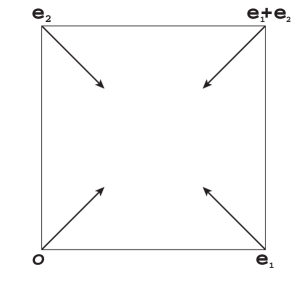
Figure 3: Spin density $\mbox{\boldmath$s$}(\mbox{\boldmath$m$})=\left(s^{1}(\mbox{\boldmath$m$}),s^{2}(\mbox{\boldmath$m$})\right)$ of the $G(XA_{g},1,1)_{3}$ state. $|\mbox{\boldmath$s$}(\mbox{\boldmath$m$})|=c+d+f$.

Example 6.5.

$G(XB_{3g},1,1)_{3}$ state.
The isotropy subgroup of the $G(XB_{3g},1,1)_{3}$ state is

$$G(XB_{3g},1,1)_{3} =M(\mbox{\boldmath$e$}_{3})T_{x}(\mbox{\boldmath$e$}_{2})T_{y}(\mbox{\boldmath$e$}_{1})\mbox{\boldmath$D$}_{4h}(u_{4z}^{+},u_{2x})\mbox{\boldmath$L$}_{3}.$$ (318)

From $G(XB_{3g},1,1)_{3}$ invariance, we obtain non-zero $\mbox{\boldmath$R$}^{00},\mbox{\boldmath$R$}^{13},\mbox{\boldmath$R$}^{21}$ and $\mbox{\boldmath$R$}^{32}$ as follows

$$\mbox{\boldmath$R$}^{00} =\left(\begin{array}[]{ccc}a&0&0\\ 0&a&0\\ 0&0&b\end{array}\right), \mbox{\boldmath$R$}^{13} =\left(\begin{array}[]{ccc}0&ic&0\\ -ic&0&0\\ 0&0&0\end{array}\right),$$ (325)

$$\mbox{\boldmath$R$}^{21} =\left(\begin{array}[]{ccc}0&0&0\\ 0&0&d\\ 0&d&0\end{array}\right), \mbox{\boldmath$R$}^{32} =\left(\begin{array}[]{ccc}0&0&-d\\ 0&0&0\\ -d&0&0\end{array}\right),$$ (332)

where $a$, $b$, $c$ and $d$ are real numbers, and $i$ is imaginary unit. From (46) and (51) we obtain, for $m$ such that $T(\mbox{\boldmath$m$})\in\mbox{\boldmath$L$}_{3}$,

$$\mbox{\boldmath$\cal{D}$}(\mbox{\boldmath$m$}) =\left(\begin{array}[]{cccccc}a&ic&0&0&0&id\\ -ic&a&0&0&0&d\\ 0&0&b&id&d&0\\ 0&0&-id&a&-ic&0\\ 0&0&d&ic&a&0\\ -id&d&0&0&0&b\end{array}\right),$$ (339)

$$\mbox{\boldmath$\cal{D}$}(\mbox{\boldmath$m$}+\mbox{\boldmath$e$}_{1}) =\left(\begin{array}[]{cccccc}a&-ic&0&0&0&id\\ ic&a&0&0&0&-d\\ 0&0&b&id&-d&0\\ 0&0&-id&a&ic&0\\ 0&0&-d&-ic&a&0\\ -id&-d&0&0&0&b\end{array}\right),$$ (346)

$$\mbox{\boldmath$\cal{D}$}(\mbox{\boldmath$m$}+\mbox{\boldmath$e$}_{2}) =\left(\begin{array}[]{cccccc}a&-ic&0&0&0&-id\\ ic&a&0&0&0&d\\ 0&0&b&-id&d&0\\ 0&0&id&a&ic&0\\ 0&0&d&-ic&a&0\\ id&d&0&0&0&b\end{array}\right),$$ (353)

$$\mbox{\boldmath$\cal{D}$}(\mbox{\boldmath$m$}+\mbox{\boldmath$e$}_{1}+\mbox{\boldmath$e$}_{2}) =\left(\begin{array}[]{cccccc}a&ic&0&0&0&-id\\ -ic&a&0&0&0&-d\\ 0&0&b&-id&-d&0\\ 0&0&id&a&-ic&0\\ 0&0&-d&ic&a&0\\ id&-d&0&0&0&b\end{array}\right).$$ (360)

Table 15: Occupied general spin orbitals and their occupation numbers for $G(XB_{3g},1,1)_{3}$ state

site	general spin orbital	occupation number
$m$	$\psi_{1}=i\frac{\mathrm{sgn}(d)}{\sqrt{2}}u(\phi_{1}-i\phi_{2})\mid\uparrow\rangle+w\phi_{3}\mid\downarrow\rangle$	$\lambda_{1}$
$m$	$\psi_{2}=-i\frac{\mathrm{sgn}(d)}{\sqrt{2}}u(\phi_{1}+i\phi_{2})\mid\downarrow\rangle+w\phi_{3}\mid\uparrow\rangle$	$\lambda_{1}$
$m$	$\psi_{3}=-i\frac{\mathrm{sgn}(d)}{\sqrt{2}}w(\phi_{1}-i\phi_{2})\mid\uparrow\rangle+u\phi_{3}\mid\downarrow\rangle$	$\lambda_{2}$
$m$	$\psi_{4}=i\frac{\mathrm{sgn}(d)}{\sqrt{2}}w(\phi_{1}+i\phi_{2})\mid\downarrow\rangle+u\phi_{3}\mid\uparrow\rangle$	$\lambda_{2}$
$m$	$\psi_{5}=\frac{1}{\sqrt{2}}(\phi_{1}+i\phi_{2})\mid\uparrow\rangle$	$\lambda_{3}$
$m$	$\psi_{6}=\frac{1}{\sqrt{2}}(\phi_{1}-i\phi_{2})\mid\downarrow\rangle$	$\lambda_{3}$
$\mbox{\boldmath$m$}+\mbox{\boldmath$e$}_{1}$	$\psi_{1}=i\frac{\mathrm{sgn}(d)}{\sqrt{2}}u(\phi_{1}+i\phi_{2})\mid\uparrow\rangle+w\phi_{3}\mid\downarrow\rangle$	$\lambda_{1}$
$\mbox{\boldmath$m$}+\mbox{\boldmath$e$}_{1}$	$\psi_{2}=-i\frac{\mathrm{sgn}(d)}{\sqrt{2}}u(\phi_{1}-i\phi_{2})\mid\downarrow\rangle+w\phi_{3}\mid\uparrow\rangle$	$\lambda_{1}$
$\mbox{\boldmath$m$}+\mbox{\boldmath$e$}_{1}$	$\psi_{3}=-i\frac{\mathrm{sgn}(d)}{\sqrt{2}}w(\phi_{1}+i\phi_{2})\mid\uparrow\rangle+u\phi_{3}\mid\downarrow\rangle$	$\lambda_{2}$
$\mbox{\boldmath$m$}+\mbox{\boldmath$e$}_{1}$	$\psi_{4}=i\frac{\mathrm{sgn}(d)}{\sqrt{2}}w(\phi_{1}-i\phi_{2})\mid\downarrow\rangle+u\phi_{3}\mid\uparrow\rangle$	$\lambda_{2}$
$\mbox{\boldmath$m$}+\mbox{\boldmath$e$}_{1}$	$\psi_{5}=\frac{1}{\sqrt{2}}(\phi_{1}-i\phi_{2})\mid\uparrow\rangle$	$\lambda_{3}$
$\mbox{\boldmath$m$}+\mbox{\boldmath$e$}_{1}$	$\psi_{6}=\frac{1}{\sqrt{2}}(\phi_{1}+i\phi_{2})\mid\downarrow\rangle$	$\lambda_{3}$
$\mbox{\boldmath$m$}+\mbox{\boldmath$e$}_{2}$	$\psi_{1}=-i\frac{\mathrm{sgn}(d)}{\sqrt{2}}u(\phi_{1}+i\phi_{2})\mid\uparrow\rangle+w\phi_{3}\mid\downarrow\rangle$	$\lambda_{1}$
$\mbox{\boldmath$m$}+\mbox{\boldmath$e$}_{2}$	$\psi_{2}=i\frac{\mathrm{sgn}(d)}{\sqrt{2}}u(\phi_{1}-i\phi_{2})\mid\downarrow\rangle+w\phi_{3}\mid\uparrow\rangle$	$\lambda_{1}$
$\mbox{\boldmath$m$}+\mbox{\boldmath$e$}_{2}$	$\psi_{3}=i\frac{\mathrm{sgn}(d)}{\sqrt{2}}w(\phi_{1}+i\phi_{2})\mid\uparrow\rangle+u\phi_{3}\mid\downarrow\rangle$	$\lambda_{2}$
$\mbox{\boldmath$m$}+\mbox{\boldmath$e$}_{2}$	$\psi_{4}=-i\frac{\mathrm{sgn}(d)}{\sqrt{2}}w(\phi_{1}-i\phi_{2})\mid\downarrow\rangle+u\phi_{3}\mid\uparrow\rangle$	$\lambda_{2}$
$\mbox{\boldmath$m$}+\mbox{\boldmath$e$}_{2}$	$\psi_{5}=\frac{1}{\sqrt{2}}(\phi_{1}-i\phi_{2})\mid\uparrow\rangle$	$\lambda_{3}$
$\mbox{\boldmath$m$}+\mbox{\boldmath$e$}_{2}$	$\psi_{6}=\frac{1}{\sqrt{2}}(\phi_{1}+i\phi_{2})\mid\downarrow\rangle$	$\lambda_{3}$
$\mbox{\boldmath$m$}+\mbox{\boldmath$e$}_{1}+\mbox{\boldmath$e$}_{2}$	$\psi_{1}=-i\frac{\mathrm{sgn}(d)}{\sqrt{2}}u(\phi_{1}-i\phi_{2})\mid\uparrow\rangle+w\phi_{3}\mid\downarrow\rangle$	$\lambda_{1}$
$\mbox{\boldmath$m$}+\mbox{\boldmath$e$}_{1}+\mbox{\boldmath$e$}_{2}$	$\psi_{2}=i\frac{\mathrm{sgn}(d)}{\sqrt{2}}u(\phi_{1}+i\phi_{2})\mid\downarrow\rangle+w\phi_{3}\mid\uparrow\rangle$	$\lambda_{1}$
$\mbox{\boldmath$m$}+\mbox{\boldmath$e$}_{1}+\mbox{\boldmath$e$}_{2}$	$\psi_{3}=i\frac{\mathrm{sgn}(d)}{\sqrt{2}}w(\phi_{1}-i\phi_{2})\mid\uparrow\rangle+u\phi_{3}\mid\downarrow\rangle$	$\lambda_{2}$
$\mbox{\boldmath$m$}+\mbox{\boldmath$e$}_{1}+\mbox{\boldmath$e$}_{2}$	$\psi_{4}=-i\frac{\mathrm{sgn}(d)}{\sqrt{2}}w(\phi_{1}+i\phi_{2})\mid\downarrow\rangle+u\phi_{3}\mid\uparrow\rangle$	$\lambda_{2}$
$\mbox{\boldmath$m$}+\mbox{\boldmath$e$}_{1}+\mbox{\boldmath$e$}_{2}$	$\psi_{5}=\frac{1}{\sqrt{2}}(\phi_{1}+i\phi_{2})\mid\uparrow\rangle$	$\lambda_{3}$
$\mbox{\boldmath$m$}+\mbox{\boldmath$e$}_{1}+\mbox{\boldmath$e$}_{2}$	$\psi_{6}=\frac{1}{\sqrt{2}}(\phi_{1}-i\phi_{2})\mid\downarrow\rangle$	$\lambda_{3}$
$\mbox{\boldmath$m$}:T(\mbox{\boldmath$m$})\in\mbox{\boldmath$L$}_{3}$
$a=R^{00}_{11}=R^{00}_{22},\ b=R^{00}_{33},\ ic=R^{13}_{12}=-R^{13}_{21},d=R^{21}_{23}=R^{21}_{32}=-R^{32}_{13}=-R^{32}_{31}$
$\lambda_{1}=\frac{a+b+c+\sqrt{(a-b+c)^{2}+8d^{2}}}{2},\ \lambda_{2}=\frac{a+b+c-\sqrt{(a-b+c)^{2}+8d^{2}}}{2},\ \lambda_{3}=a-c$
$u=\frac{1}{\sqrt{2}}(1+\frac{a-b+c}{\sqrt{(a-b+c)^{2}+8d^{2}}})^{\frac{1}{2}},\ w=\frac{1}{\sqrt{2}}(1-\frac{a-b+c}{\sqrt{(a-b+c)^{2}+8d^{2}}})^{\frac{1}{2}}$

Diagonalizing $\cal{D}$, we obtain the occupied general spin orbital and their occupation numbers as shown in Table 15. From (71) we see that this state has spin orbital angular momenta $l^{3}_{z}(\mbox{\boldmath$m$})$ and spin quadrupole momenta $Q^{1}_{23}(\mbox{\boldmath$m$}),Q^{2}_{31}(\mbox{\boldmath$m$})$ as follows:

$$Q^{1}_{23}(\mbox{\boldmath$m$}) =2I_{2}d,\ \ \ Q^{2}_{31}(\mbox{\boldmath$m$})=-2I_{2}d,$$

$$Q^{1}_{23}(\mbox{\boldmath$m$}+\mbox{\boldmath$e$}_{1}) =-2I_{2}d,\ \ \ Q^{2}_{31}(\mbox{\boldmath$m$}+\mbox{\boldmath$e$}_{1})=-2I_{2}d,$$

$$Q^{1}_{23}(\mbox{\boldmath$m$}+\mbox{\boldmath$e$}_{2}) =2I_{2}d,\ \ \ Q^{2}_{31}(\mbox{\boldmath$m$}+\mbox{\boldmath$e$}_{2})=-2I_{2}d,$$

$$Q^{1}_{23}(\mbox{\boldmath$m$}+\mbox{\boldmath$e$}_{1}+\mbox{\boldmath$e$}_{2}) =-2I_{2}d,\ \ \ Q^{2}_{31}(\mbox{\boldmath$m$}+\mbox{\boldmath$e$}_{1}+\mbox{\boldmath$e$}_{2})=2I_{2}d,$$

$$l_{3}^{3}(\mbox{\boldmath$m$}) =l^{3}_{3}(\mbox{\boldmath$m$}+\mbox{\boldmath$e$}_{1}+\mbox{\boldmath$e$}_{2})=2c,$$

$$l_{3}^{3}(\mbox{\boldmath$m$}+\mbox{\boldmath$e$}_{1}) =l^{3}_{3}(\mbox{\boldmath$m$}+\mbox{\boldmath$e$}_{2})=-2c,$$ (361)

for $m$ such taht $T(\mbox{\boldmath$m$})\in\mbox{\boldmath$L$}_{3}$. Here we note that the secondary LOP:$l_{3}^{3}$ is induced by the appearance of the primary LOP:$\{Q_{23}^{1},Q_{31}^{2}\}$. From (71) we can see that for all site $m$

$$s^{1}(\mbox{\boldmath$m$}) =s^{2}(\mbox{\boldmath$m$})=s^{3}(\mbox{\boldmath$m$})=0,$$

$$l_{3}(\mbox{\boldmath$m$}) =0,$$

$$Q_{23}(\mbox{\boldmath$m$}) =Q_{31}(\mbox{\boldmath$m$})=0.$$ (362)

Thus the $G(XB_{3g},1,1)_{3}$ state is not a coexistent state of spin density and quadrupole moment.

Finally we note that many states in Table 9 and 10 have spin orbital angular momentum and/or spin quadrupole moment, however they are not coexistent states of {spin density}, and {orbital angular momentum or quadrupole moment} except $G(XA_{g},1,1)_{1}$ state.

7 Some numerical results

In this section we present some calculated results of HF equations for the states listed in Table 5, Table 6, Table 9 and Table 10. We solve the Hartree-Fock equation of a state (characterized by an isotropy subgroup $G_{j}$) self-consistently by starting initial values of $\mbox{\boldmath$R$}^{l\lambda}$ with $G_{j}$ symmetry. From the SCF condition (28) we obtain the initial values of $\mbox{\boldmath$x$}^{l\lambda}$. After diagonalizing $H_{m}$ of (30) with these $\mbox{\boldmath$x$}^{l\lambda}$, we obtain new $\mbox{\boldmath$R$}^{l\lambda}$. The obtained $\mbox{\boldmath$R$}^{l\lambda}$ are substituted into (28) to compute new $\mbox{\boldmath$x$}^{l\lambda}$. We use them as inputs to repeat the above process until the relative errors in $\mbox{\boldmath$R$}^{l\lambda}$ between successive iterations are less than the desired accuracy. After obtaining converged $\mbox{\boldmath$R$}^{l\lambda}$ , we obtain the HF energy $E_{\rm HF}$ from (32).

We consider the cases of parameter sets listed in Table 16. Since it is known that Ca_2-xSr_xRuO₄ has four 4d electrons in the $\mathrm{t_{2g}}$ orbitals [4, 5], we use number of electrons per site $n_{e}^{0}=4.0$ for all parameter sets. The eighth column denotes the most stable state among all states listed in listed in Table 5, Table 6, Table 9 and Table 10.

Table 16: Parameter sets for model calculations

N.O	$\delta$	$t_{1}$	$t_{2}$	$t_{3}$	$U$	$J=J^{\prime}$	most stable state
(1)	0.0	1.0	0.0	1.0	9.0	2.25	$G(\Gamma A_{1g},1,1)$
(2)	0.4	1.0	0.0	1.0	9.0	0.4	$G(MB_{1g},1,1)$
(3)	0.0	1.0	0.0	1.0	9.0	0.7	$G(ME_{g},1,1)_{3},G(XB_{3g},1,1)_{3}$
(4)	-0.14	1.0	0.8	0.8	8.0	1.0	$G(XA_{g},1,1)_{3}$
number of electrons per site = $n_{e}^{0}=4.0,\ U^{\prime}=U-2J$

7.1 Parameter set (1)

In the parameter set (1), where $J$ has rather large values, the $G(\Gamma A_{1g},1,1)$ state is most stable. The calculated values of $a,b,c$ and $d$ in (213) are

$$a =0.6679,\ \ b=0.6643,\ \ c=0.3321,\ \ d=0.3357.$$ (363)

Thus we obtain $a+c\approx 1.0,a-c\approx\frac{1}{3},b+d\approx 1.0$ and $b-d\approx\frac{1}{3}$. Then from Table 11, the occupation numbers for $\phi_{i}\mid\uparrow\rangle$ and $\phi_{i}\mid\downarrow\rangle$ are

$$n(\phi_{1}\mid\uparrow\rangle) =n(\phi_{2}\mid\uparrow\rangle)=n(\phi_{3}\mid\uparrow\rangle)=1,$$

$$n(\phi_{1}\mid\downarrow\rangle) =n(\phi_{2}\mid\downarrow\rangle)=n(\phi_{3}\mid\downarrow\rangle)\approx\frac{1}{3}.$$ (364)

7.2 Parameter set (2)

In the parameter set (2), the $G(MB_{1g},1,1)$ state is most stable. The calculated values of $a,b$ and $c$ are

$$a =0.5,\ \ b=1,\ \ c=-0.473.$$ (365)

Thus we have

$$a+c =0.027\approx 0.0,\ \ a-c=0.974\approx 1.0,\ \ b=1.0.$$ (366)

From Table 12, we obtain a qualitative pattern of the electron occupations as shown in Fig.4.

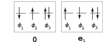
Figure 4: Schematic pattern of the electron occupation in $G(MB_{1g},1,1)$ state. $\uparrow(\downarrow)$ indicates one electron with up(down) spin.

7.3 Parameter set (3)

In the parameter set (3), the $G(ME_{g},1,1)_{3}$ and the $G(XB_{3g},1,1)_{3}$ states have the same energy and are most stable. The calculated values of $a,b,c$ and $d$ in (261) and (332) are

$$a =0.7113,\ \ b=0.5775,\ \ c=-0.2775,\ \ d=0.3240.$$ (367)

Then the occupation numbers for general spin orbitals $\psi_{j}\ (j=1,\dots,6)$ in Table 13 and 15 are

$$n(\psi_{1}) =n(\psi_{2})=\lambda_{1}=\frac{a+b+c+\sqrt{(a-b+c)^{2}+8d^{2}}}{2}\approx 1.0,$$

$$n(\psi_{3}) =n(\psi_{4})=\lambda_{2}=\frac{a+b+c-\sqrt{(a-b+c)^{2}+8d^{2}}}{2}\approx 0.0,$$

$$n(\psi_{5}) =n(\psi_{6})=\lambda_{3}=a-c\approx 1.0.$$ (368)

7.4 Parameter set (4)

In the parameter set (4), the $G(XA_{g},1,1)_{3}$ state is most stable. The calculated values of $a,b,c,d$ and $f$ in (288) are

$$a =0.75,\ \ b=0.5,\ \ c=-0.1802,\ \ d=-0.1408,\ \ f=0.3416.$$ (369)

Then the occupation numbers for general spin orbitals $\psi_{j}\ (j=1,\cdots,6)$ in Table 14 are

$$n(\psi_{1}) =n(\psi_{2})=\lambda_{1}=a+\sqrt{c^{2}+d^{2}}=0.9786\approx 1.0,$$

$$n(\psi_{3}) =n(\psi_{4})=\lambda_{2}=a-\sqrt{c^{2}+d^{2}}=0.521\approx 0.5,$$

$$n(\psi_{5}) =\lambda_{3}=b+\sqrt{2}f=0.017\approx 0.0,$$

$$n(\psi_{6}) =\lambda_{4}=b-\sqrt{2}f=0.983\approx 1.0.$$ (370)

The magnitude of spin density $|\mbox{\boldmath$s$}(\mbox{\boldmath$m$})|$ is $c+d+f=-0.1802-0.1408+0.3416=0.0206$.

8 Summary and discussion

We applied the group theoretical bifurcation theory of the HF equation to the $\mathrm{t_{2g}}$-Hubbard model on a two-dimensional square lattice. By enumerating the axial isotropy subgroups of the R-reps of the group $G_{0}$ in the HF Hamiltonian space $W_{\rm HF}$ in the cases of ordering vectors $\mbox{\boldmath$Q$}_{i},i=0,1,2,3$, we have obtained many types of broken symmetry states which bifurcate from the normal state through one step transition.

It is shown that these states have various types of local order parameters (LOP): spin density $\mbox{\boldmath$s$}=(s^{1},s^{2},s^{3})$, quadrupole moment $\mbox{\boldmath$Q$}=(Q_{2}^{2},Q_{12},Q_{23},Q_{31})$, orbital angular momentum $\mbox{\boldmath$l$}=(l_{1},l_{2},l_{3})$, spin quadrupole moment $\mbox{\boldmath$Q$}^{\lambda}=(Q_{2}^{2\lambda},Q_{12}^{\lambda},Q_{23}^{\lambda},Q_{31}^{\lambda})$ and spin orbital angular momentum $\mbox{\boldmath$l$}^{\lambda}=(l_{1}^{\lambda},l_{2}^{\lambda},l_{3}^{\lambda})$, where $\lambda=1,2,3$. We have illustrated how the isotropy subgroup of a state can determine the canonical form of the HF Hamiltonian, the standard forms of the occupied spin orbitals and their occupation number, and types of LOP.

We performed numerical calculations for all states discussed in §5 and §6 with some parameter sets. We found that various types of broken symmetric solutions can be the most stable state depending on parameter sets. Through these calculations we found that non-collinear magnetic states:$G(ME_{g},1,1)_{3},G(XB_{3g},1,1)_{3}$ and $G(XA_{g},1,1)_{3}$ can be the ground state for some parameter sets.

In §5 and §6 we considered broken symmetry states bifurcating through a single phase transition from the normal state. However as shown in §7 of I, there are many other states derived through two step transitions from the normal state. Here we consider two states bifurcatig from the $G(MB_{2g},0,0)$ treated in the Example 5.2. The isotropy subgroup of the $G(MB_{2g},0,0)$ is

$$G(MB_{2g},0,0)=\left(E+T(\mbox{\boldmath$e$}_{1})C_{2x}\right)\mbox{\boldmath$D$}_{2a}\mbox{\boldmath$L$}_{1}\mbox{\boldmath$S$}\mbox{\boldmath$R$}$$ (371)

By a similar method to that in §7 of the previous paper, we obtain the following two types of isotropic subgroups

$$G(MB_{2g},0,0)_{a} =(E+tu_{2y})(E+T(\mbox{\boldmath$e$}_{1})C_{2x})\mbox{\boldmath$D$}_{2ah}\mbox{\boldmath$L$}_{1}\mbox{\boldmath$A$}(\mbox{\boldmath$e$}_{3}),$$

$$G(MB_{2g},0,0)_{b} =(E+tu_{2y})(E+T(\mbox{\boldmath$e$}_{1})C_{2x}u_{2x})\mbox{\boldmath$D$}_{2ah}\mbox{\boldmath$L$}_{1}\mbox{\boldmath$A$}(\mbox{\boldmath$e$}_{3}).$$ (372)

We consider these states seperately.
(a) $G(MB_{2g},0,0)_{a}$ state.
This state has following non zero $\mbox{\boldmath$R$}^{l\nu}$

$$\mbox{\boldmath$R$}^{00} =\left(\begin{array}[]{ccc}a&0&0\\ 0&a&0\\ 0&0&b\end{array}\right),\ \ \mbox{\boldmath$R$}^{10}=\left(\begin{array}[]{ccc}0&c&0\\ c&0&0\\ 0&0&0\end{array}\right),$$ (379)

$$\mbox{\boldmath$R$}^{03} =\left(\begin{array}[]{ccc}d&0&0\\ 0&d&0\\ 0&0&f\end{array}\right),\ \ \mbox{\boldmath$R$}^{13}=\left(\begin{array}[]{ccc}0&e&0\\ e&0&0\\ 0&0&0\end{array}\right).$$ (386)

Thus from (71) we obtain for $m$ such that $T(\mbox{\boldmath$m$})\in\mbox{\boldmath$L$}_{1}$

$$Q_{12}(\mbox{\boldmath$m$}) =4I_{2}c,\ \ \ Q_{12}(\mbox{\boldmath$m$}+\mbox{\boldmath$e$}_{j})=-4I_{2}c,$$

$$s^{3}(\mbox{\boldmath$m$}) =2d+f,\ \ s^{3}(\mbox{\boldmath$m$}+\mbox{\boldmath$e$}_{j})=2d+f,$$

$$Q_{12}^{3}(\mbox{\boldmath$m$}) =2I_{2}e,\ \ \ Q_{12}^{3}(\mbox{\boldmath$m$}+\mbox{\boldmath$e$}_{j})=-2I_{2}e,$$ (387)

where $j=1,2$. Thus we see that through the ferromagnetic transition of the $G(MB_{2g},0,0)$ state which has the anti-ferro quadrupole moment $Q_{12}$, there appears anti-ferro spin quadrupole moment $Q_{12}^{3}$ as well as ferro spin density $s^{3}$.

(b) $G(MB_{2g},0,0)_{b}$ state.
This state has following non zero $\mbox{\boldmath$R$}^{l\nu}$

$$\mbox{\boldmath$R$}^{00} =\left(\begin{array}[]{ccc}a&0&0\\ 0&a&0\\ 0&0&b\end{array}\right)\ \ \mbox{\boldmath$R$}^{10}=\left(\begin{array}[]{ccc}0&c&0\\ c&0&0\\ 0&0&0\end{array}\right)$$ (394)

$$\mbox{\boldmath$R$}^{03} =\left(\begin{array}[]{ccc}0&e&0\\ e&0&0\\ 0&0&f\end{array}\right)\ \ \mbox{\boldmath$R$}^{13}=\left(\begin{array}[]{ccc}d&0&0\\ 0&d&0\\ 0&0&f\end{array}\right)$$ (401)

Thus we obtain, for $m$ such that $T(\mbox{\boldmath$m$})\in\mbox{\boldmath$L$}_{1}$ and $j=1,2$,

$$Q_{12}(\mbox{\boldmath$m$}) =4I_{2}c,\ \ \ Q_{12}(\mbox{\boldmath$m$}+\mbox{\boldmath$e$}_{j})=-4I_{2}c,$$

$$s^{3}(\mbox{\boldmath$m$}) =2d+f,\ \ s^{3}(\mbox{\boldmath$m$}+\mbox{\boldmath$e$}_{j})=-(2d+f),$$

$$Q_{12}^{3}(\mbox{\boldmath$m$}) =2I_{2}e,\ \ \ Q_{12}^{3}(\mbox{\boldmath$m$}+\mbox{\boldmath$e$}_{j})=2I_{2}e.$$ (402)

Thus we see that through the anti-ferromagnetic transition of the $G(MB_{2g},0,0)$ state, there appears ferro spin quadrupole moment $Q_{12}^{3}$ as well as anti-ferro spin density $s^{3}$.

By similar manner to that of above cases, we can see that states, which are derived through two step transition from the normal state, are coexisting states of {spin sensity , quadrupole moment and spin quadrupole moment }, or {spin sensity, orbital angular momentum and spin orbital angular momentum}.

Appendix A Derivation of quadrupole moment

Here we derive (64) for the quadrupole moment at the site $m$. The quadrupole moment operator $\hat{Q}_{ij}(\mbox{\boldmath$m$})$ at a site $m$ is defined by[22]

$$\hat{\cal{Q}}_{ij}(\mbox{\boldmath$m$}) =\sum_{p,q=1}^{3}\sum_{s,s^{\prime}=1}^{2}\langle\phi_{\mbox{\scriptsize\boldmath$m$}ps}|(3x_{i}x_{j}-\delta_{ij}r^{2})|\phi_{\mbox{\scriptsize\boldmath$m$}qs^{\prime}}\rangle a^{{\dagger}}_{\mbox{\scriptsize\boldmath$m$}ps}a_{\mbox{\scriptsize\boldmath$m$}qs^{\prime}}$$

$$=\sum_{s=1}^{2}\sum_{p,q=1}^{3}(\mbox{\boldmath$\cal{Q}$}_{ij})_{pq}a^{{\dagger}}_{\mbox{\boldmath$m$}ps}a_{\mbox{\boldmath$m$}qs},$$ (403)

where $\phi_{\mbox{\scriptsize\boldmath$m$}ps}=\phi_{p}(\mbox{\boldmath$r$}-\mbox{\boldmath$m$})\chi_{s}$, $\chi_{s}$ are the spin function: $\chi_{1}=|\uparrow\rangle,\chi_{2}=|\downarrow\rangle$, and $\mbox{\boldmath$\cal{Q}$}_{ij}$ is a $3\times 3$ symmetric matrix whose ($p,q$) component is defined by

$$\left(\mbox{\boldmath$\cal{Q}$}_{ij}\right)_{pq} =\int d\mbox{\boldmath$r$}\phi_{p}(\mbox{\boldmath$r$})(3x_{i}x_{j}-r^{2}\delta_{ij})\phi_{q}(\mbox{\boldmath$r$}).$$ (404)

Thus the expectation value of the quadrupole moment at a site $m$ given by

$$Q_{ij}(\mbox{\boldmath$m$}) =\sum_{s=1}^{2}\sum_{p,q=1}^{3}(\mbox{\boldmath$\cal{Q}$}_{ij})_{pq}\langle a^{{\dagger}}_{\mbox{\boldmath$m$}ps}a_{\mbox{\boldmath$m$}qs}\rangle.$$ (405)

The explicit forms of $\mbox{\boldmath$\cal{Q}$}_{ij}$ are given by

$$\mbox{\boldmath$\cal{Q}$}_{11} =\left(\begin{array}[]{ccc}2I_{1}&0&0\\ 0&-I_{1}&0\\ 0&0&-I_{1}\end{array}\right),\quad\mbox{\boldmath$\cal{Q}$}_{12}=\mbox{\boldmath$Q$}_{21}=\left(\begin{array}[]{ccc}0&I_{2}&0\\ I_{2}&0&0\\ 0&0&0\end{array}\right),$$ (412)

$$\mbox{\boldmath$\cal{Q}$}_{22} =\left(\begin{array}[]{ccc}-I_{1}&0&0\\ 0&2I_{1}&0\\ 0&0&-I_{1}\end{array}\right),\quad\mbox{\boldmath$\cal{Q}$}_{23}=\mbox{\boldmath$Q$}_{32}=\left(\begin{array}[]{ccc}0&0&0\\ 0&0&I_{2}\\ 0&I_{2}&0\end{array}\right),$$ (419)

$$\mbox{\boldmath$\cal{Q}$}_{33} =\left(\begin{array}[]{ccc}-I_{1}&0&0\\ 0&-I_{1}&0\\ 0&0&2I_{1}\end{array}\right),\quad\mbox{\boldmath$\cal{Q}$}_{31}=\mbox{\boldmath$Q$}_{31}=\left(\begin{array}[]{ccc}0&0&I_{2}\\ 0&0&0\\ I_{2}&0&0\end{array}\right),$$ (426)

where

$$I_{1} =\int d\mbox{\boldmath$r$}\phi_{1}(\mbox{\boldmath$r$})(x^{2}-y^{2})\phi_{1}(\mbox{\boldmath$r$}),$$

$$I_{2} =3\int d\mbox{\boldmath$r$}\phi_{1}(\mbox{\boldmath$r$})xy\phi_{2}(\mbox{\boldmath$r$}).$$ (427)

Thus from(405) and (426) we obtain

$$Q_{11}(\mbox{\boldmath$m$}) =I_{1}\sum_{s,s^{\prime}=1}^{2}\left(2\langle a^{{\dagger}}_{\mbox{\scriptsize\boldmath$m$}1s}a_{\mbox{\scriptsize\boldmath$m$}1s^{\prime}}\rangle-\langle a^{{\dagger}}_{\mbox{\scriptsize\boldmath$m$}2s}a_{\mbox{\scriptsize\boldmath$m$}2s^{\prime}}\rangle-\langle a^{{\dagger}}_{\mbox{\scriptsize\boldmath$m$}3s}a_{\mbox{\scriptsize\boldmath$m$}3s^{\prime}}\rangle\right)\sigma^{0}_{ss^{\prime}},$$

$$Q_{22}(\mbox{\boldmath$m$}) =I_{1}\sum_{s,s^{\prime}=1}^{2}\left(-\langle a^{{\dagger}}_{\mbox{\scriptsize\boldmath$m$}1s}a_{\mbox{\scriptsize\boldmath$m$}1s^{\prime}}\rangle+2\langle a^{{\dagger}}_{\mbox{\scriptsize\boldmath$m$}2s}a_{\mbox{\scriptsize\boldmath$m$}2s^{\prime}}\rangle-\langle a^{{\dagger}}_{\mbox{\scriptsize\boldmath$m$}3s}a_{\mbox{\scriptsize\boldmath$m$}3s^{\prime}}\rangle\right)\sigma^{0}_{ss^{\prime}},$$

$$Q_{33}(\mbox{\boldmath$m$}) =I_{1}\sum_{s,s^{\prime}=1}^{2}\left(-\langle a^{{\dagger}}_{\mbox{\scriptsize\boldmath$m$}1s}a_{\mbox{\scriptsize\boldmath$m$}1s^{\prime}}\rangle-\langle a^{{\dagger}}_{\mbox{\scriptsize\boldmath$m$}2s}a_{\mbox{\scriptsize\boldmath$m$}2s^{\prime}}\rangle+2\langle a^{{\dagger}}_{\mbox{\scriptsize\boldmath$m$}3s}a_{\mbox{\scriptsize\boldmath$m$}3s^{\prime}}\rangle\right)\sigma^{0}_{ss^{\prime}},$$

$$Q_{12}(\mbox{\boldmath$m$}) =Q_{21}(\mbox{\boldmath$m$})=I_{2}\sum_{s,s^{\prime}=1}^{2}\left(\langle a^{{\dagger}}_{\mbox{\scriptsize\boldmath$m$}1s}a_{\mbox{\scriptsize\boldmath$m$}2s^{\prime}}\rangle+\langle a^{{\dagger}}_{\mbox{\scriptsize\boldmath$m$}2s}a_{\mbox{\scriptsize\boldmath$m$}1s^{\prime}}\rangle\right)\sigma^{0}_{ss^{\prime}},$$

$$Q_{23}(\mbox{\boldmath$m$}) =Q_{32}(\mbox{\boldmath$m$})=I_{2}\sum_{s,s^{\prime}=1}^{2}\left(\langle a^{{\dagger}}_{\mbox{\scriptsize\boldmath$m$}2s}a_{\mbox{\scriptsize\boldmath$m$}3s^{\prime}}\rangle+\langle a^{{\dagger}}_{\mbox{\scriptsize\boldmath$m$}3s}a_{\mbox{\scriptsize\boldmath$m$}2s^{\prime}}\rangle\right)\sigma^{0}_{ss^{\prime}},$$

$$Q_{31}(\mbox{\boldmath$m$}) =Q_{13}(\mbox{\boldmath$m$})=I_{2}\sum_{s,s^{\prime}=1}^{2}\left(\langle a^{{\dagger}}_{\mbox{\scriptsize\boldmath$m$}3s}a_{\mbox{\scriptsize\boldmath$m$}1s^{\prime}}\rangle+\langle a^{{\dagger}}_{\mbox{\scriptsize\boldmath$m$}1s}a_{\mbox{\scriptsize\boldmath$m$}3s^{\prime}}\rangle\right)\sigma^{0}_{ss^{\prime}}.$$ (428)

The spin quadrupole moment is defined by

$$\hat{\cal{Q}}^{\lambda}_{ij}(\mbox{\boldmath$m$}) =\dfrac{1}{2}\sum_{p,q=1}^{3}\sum_{s,s^{\prime}=1}^{2}\langle\phi_{\mbox{\scriptsize\boldmath$m$}ps}|(3x_{i}x_{j}-\delta_{ij}r^{2})\sigma^{\lambda}_{ss^{\prime}}|\phi_{\mbox{\scriptsize\boldmath$m$}qs^{\prime}}\rangle a^{{\dagger}}_{\mbox{\scriptsize\boldmath$m$}ps}a_{\mbox{\scriptsize\boldmath$m$}qs^{\prime}}.$$ (429)

Then we obtain (66) for the expectation values of spin quadrupole moment.

Appendix B Derivation of the orbital angular momentum

Here we derive (68) for the orbital angular momentum at the site $m$. Let $\hat{l}_{j}~{}(j=1,2,3)$ be the orbital angular momentum. Then operators of the orbital angular mormentum at the site $m$ are expressed by

$$\hat{l}_{i}(\mbox{\boldmath$m$}) =\sum_{p,q=1}^{3}\sum_{s,s^{\prime}=1}^{2}\langle\phi_{\mbox{\scriptsize\boldmath$m$}ps}|\hat{l}_{i}|\phi_{\mbox{\scriptsize\boldmath$m$}qs^{\prime}}\rangle a^{{\dagger}}_{\mbox{\scriptsize\boldmath$m$}ps}a_{\mbox{\scriptsize\boldmath$m$}qs^{\prime}}$$

$$=\sum_{p,q=1}^{3}\sum_{s=1}^{2}\langle\phi_{\mbox{\scriptsize\boldmath$m$}ps}|\hat{l}_{i}|\phi_{\mbox{\scriptsize\boldmath$m$}qs}\rangle a^{{\dagger}}_{\mbox{\scriptsize\boldmath$m$}ps}a_{\mbox{\scriptsize\boldmath$m$}qs}$$

$$=\sum_{p,q=1}^{3}\sum_{s=1}^{2}(L_{i})_{pq}a^{{\dagger}}_{\mbox{\scriptsize\boldmath$m$}ps}a_{\mbox{\scriptsize\boldmath$m$}qs}.$$ (430)

where

$$(L_{i})_{pq} =\langle\phi_{\mbox{\scriptsize\boldmath$m$}ps}|\hat{l}_{i}|\phi_{\mbox{\scriptsize\boldmath$m$}qs}\rangle.$$ (431)

We denote a $3\times 3$ matrix, whose $(p,q)$ component is $(L_{i})_{pq}$, by $L_{i}$. Within the $\mathrm{t_{2g}}$ subspace we have [23]

$$L_{1} =\left(\begin{array}[]{ccc}0&0&0\\ 0&0&i\\ 0&-i&0\end{array}\right),\ L_{2}=\left(\begin{array}[]{ccc}0&0&-i\\ 0&0&0\\ i&0&0\end{array}\right),\ L_{3}=\left(\begin{array}[]{ccc}0&i&0\\ -i&0&0\\ 0&0&0\end{array}\right).$$ (441)

Thus form (430) and (441) the expectation values $l_{i}(\mbox{\boldmath$m$})$ of the orbital angular momentum $\hat{l}_{i}(\mbox{\boldmath$m$})$ are given by

$$l_{1}(\mbox{\boldmath$m$}) =\sum_{ss^{\prime}}(i)(\langle a^{{\dagger}}_{\mbox{\boldmath$m$}2s}a_{\mbox{\scriptsize\boldmath$m$}3s^{\prime}}\rangle-\langle a^{{\dagger}}_{\mbox{\boldmath$m$}3s}a_{\mbox{\scriptsize\boldmath$m$}2s^{\prime}}\rangle)\sigma^{0}_{ss^{\prime}},$$

$$l_{2}(\mbox{\boldmath$m$}) =\sum_{ss^{\prime}}(i)(\langle a^{{\dagger}}_{\mbox{\boldmath$m$}3s}a_{\mbox{\scriptsize\boldmath$m$}1s^{\prime}}\rangle-\langle a^{{\dagger}}_{\mbox{\boldmath$m$}1s}a_{\mbox{\scriptsize\boldmath$m$}3s^{\prime}}\rangle)\sigma^{0}_{ss^{\prime}},$$

$$l_{3}(\mbox{\boldmath$m$}) =\sum_{ss^{\prime}}(i)(\langle a^{{\dagger}}_{\mbox{\boldmath$m$}1s}a_{\mbox{\scriptsize\boldmath$m$}2s^{\prime}}\rangle-\langle a^{{\dagger}}_{\mbox{\boldmath$m$}2s}a_{\mbox{\scriptsize\boldmath$m$}1s^{\prime}}\rangle)\sigma^{0}_{ss^{\prime}}.$$ (442)

The spin orbital angular momentum is defined by

$$\hat{l}^{\lambda}_{i}(\mbox{\boldmath$m$}) =\dfrac{1}{2}\sum_{p,q=1}^{3}\sum_{s,s^{\prime}=1}^{2}\langle\phi_{\mbox{\scriptsize\boldmath$m$}ps}|\hat{l}_{i}\sigma^{\lambda}_{ss^{\prime}}|\phi_{\mbox{\scriptsize\boldmath$m$}qs^{\prime}}\rangle a^{{\dagger}}_{\mbox{\scriptsize\boldmath$m$}ps}a_{\mbox{\scriptsize\boldmath$m$}qs^{\prime}}.$$ (443)

Then we obtain (69) for the spin orbital angular momenta.

References

- [1] T. Mizokawa and A. Fujimori: \PRB54,1996,5368.
- [2] Y. Ren, A. A.Nugroho, A. A. Menovsky, J. Strempher, U. Rutt, F. Iga, T. Takabatake and C. W. Kimball: \PRB67,2003,014107.
- [3] M. Mochizuki and M. Imada:\JPSJ73,2004,1833.
- [4] M. Kubota, Y. Murakami, M. Mizumaki, H. Ohsumi, N. Ikeda, S. Nakatsuji, H. Fukazawa and Y. Maeno: \PRL95,2005,026401.
- [5] T. Hotta and E. Dagotto: \PRL88,2002,017201.
- [6] M. Kurokawa and T. Mizokawa: \PRB66,2002,024434.
- [7] V. I. Anisimov, I. A. Nekrasov, D. E. Kondakov, T. M. Rice and M. Sigrist: Eur. Phys. J. B25(2002),191.
- [8] Z. Fang, N. Nagaosa, and K. Terakura: \PRB69,2004,045116.
- [9] A. Nakanishi, M. Hamada, A. Goto and M. Ozaki: \PTP118,2007,413.
- [10] H. Fukutome: \PTP52,1974,115; Int. J. Quantum Chem. 20 (1981),955.
- [11] M. Ozaki: \JMP26,1985,1514.
- [12] M. Ozaki: Int. J. Quantum Chem. 42 (1992),55.
- [13] M. Ozaki: \PTP67,1982,83, 415.
- [14] A. Masago, S. Mori and M. Ozaki: \IJMPB14,2000,2241.
- [15] M. Golubitsky and D. G. Schaeffer: Singurality and Groups in Bifurcation Theory, Vol. I, Applied Mathematical Sciences 51. (Springer-Verlag, New York, 1985).
- [16] M. Golubitsky, I. Stewart and D. G. Schaeffer: Singurality and Groups in Bifurcation Theory, Vol. II, Applied Mathematical Sciences 69. (Springer-Verlag, New York, 1988).
- [17] M. Golubittsky and I. Stewart: The Symmetry Perspective, (Birkhäuser, 2002).
- [18] D. H. Sattinger: Group Theoretic Methods in Bifurcation Theory, Lecture Notes in Mathematics 762 (Springer-Verlag, Berlin, 1979).
- [19] M. Ozaki: Bussei Kenkyuu 78 (2002) 511; 80 (2003) 205; 82 (2003) 479 [in Japanese].
- [20] J. F. Cornwell: Group Theory in Physics, II (Academic Press,1984), p.434.
- [21] R. Shiina, T. Nishitani and H. Shiba :\JPSJ66,1997,3159.
- [22] G. Uimin: \PRB55,1997,8267.
- [23] K. Kamimura, S. Sugano and Y. Tanabe: Hai-ishiba Riron to Sono Ouyou(Ligand Field Theory and Its Applications) (Syokabo, Tokyo, 1969) p.91 [In Japanese].