Thermodynamics and linear response of a Bose-Einstein condensate of microcavity polaritons

Abstract

In this work we derive a theory of polariton condensation based on the theory of interacting Bose particles. In particular, we describe self-consistently the linear exciton-photon coupling and the exciton-nonlinearities, by generalizing the Hartree-Fock-Popov description of BEC to the case of two coupled Bose fields at thermal equilibrium. In this way, we compute the density-dependent one-particle spectrum, the energy occupations and the phase diagram. The results quantitatively agree with the existing experimental findings. We then present the equations for the linear response of a polariton condensate and we predict the spectral response of the system to external optical or mechanical perturbations.

I Introduction

An important advance in the investigation of quantum fluids was recently achieved with the experimental observation of high quantum degeneracy and off-diagonal long-range coherence, in a gas of exciton- polaritons in a two-dimensional semiconductor microcavity Kasprzak et al. (2006); Balili et al. (2007). High quantum degeneracy has been also observed in long-living polariton systems close to thermal equilibrium Deng et al. (2006). Bose-Einstein condensation (BEC) is the most natural way of describing these findings. However, due to the peculiarity of the polariton system, in particular the finite polariton lifetime, the intrinsic 2-D nature and the presence of interface disorder, the existing theoretical frameworks rather interpret the phenomenon in strict analogy either with laser physics Laussy et al. (2004); Schwendimann and Quattropani (2006) or with the BCS transition of Fermi particles Keeling et al. (2004); Marchetti et al. (2006); Szymanska et al. (2006). In particular, the problem of the polariton kinetics and of the non-equilibrium effects, due to the finite polariton lifetime and the relaxation bottleneck, have been investigated in many works Schwendimann and Quattropani (2006); Szymanska et al. (2006); Doan et al. (2005); Sarchi and Savona (2006); Wouters and Carusotto (2007). From these studies, the main effect of non-equilibrium seems to be a significant depletion of the condensate - with corresponding loss of long-range coherence - Sarchi and Savona (2007a) and the appearance of a diffusive excitation spectrum at low momenta Szymanska et al. (2006); Wouters and Carusotto (2007).

In spite of the high relevance of these theoretical descriptions, two basic questions remain still unanswered. Are the experimental findings correctly interpreted in terms of a quantum field theory of interacting bosons? Could the achievement of polariton BEC give new insights into the fundamental physics of interacting Bose systems?

In this work we tackle these two questions, by showing that polaritons can be modeled borrowing from the theory of interacting Bose particles. In particular, we describe self-consistently the linear exciton-photon coupling and the exciton-nonlinearities, by generalizing the Hartree-Fock-Popov (HFP) description of BEC to the case of two coupled Bose fields at thermal equilibrium. In this way, we compute the density-dependent energy shifts and the phase diagram and we find a very good agreement with the recent experimental findings. Then, we apply the present theory to derive the full set of equations describing the density-density response of the polariton condensate to an external perturbation. Focusing on the photon density response, which is directly related to photoluminescence, we predict different response of the collective modes to optical (light) or mechanical (coherent phonons) perturbations. Since this behavior is driven by the presence of a coherent exciton field, we suggest that an experiment investigating these features could possibly solve the tricky problem of assessing the nature of the polariton condensate.

II Theory

The physics of the polariton system is basically that of two linearly coupled oscillators, the exciton and the cavity photon fields Savona and Tassone (1995); Savona et al. (1999). Considering the limit of low density, the exciton field can be treated as a Bose field, subject to two kinds of interactions, the mutual exciton-exciton interaction and the effective exciton-photon interaction, originating from the saturation of the exciton oscillator strength Laikhtman (2007). Therefore, to describe polariton BEC we extend to the case of two coupled interacting Bose fields the formalism adopted in describing the BEC of a single Bose field Shi and Griffin (1998); Pitaevskii and Stringari (2003).

We express the exciton and photon field operators in the Heisenberg representation via the notation

$$\hat{\Psi}_{x}({\bf r},t)=\frac{1}{\sqrt{A}}\sum_{\bf k}e^{i{\bf k}\cdot{\bf r}}\hat{b}_{\bf k}(t)\,,$$ (1)

and

$$\hat{\Psi}_{c}({\bf r},t)=\frac{1}{\sqrt{A}}\sum_{\bf k}e^{i{\bf k}\cdot{\bf r}}\hat{c}_{\bf k}(t)\,,$$ (2)

where $A$ is the system area, while $\hat{b}_{\bf k}$ and $\hat{c}_{\bf k}$ are independent Bose operators $([\hat{b}_{\bf k},\hat{c}_{\bf k^{\prime}}^{\dagger}]=0)$. Notice that in this work we assume scalar exciton and photon fields. However, the theory can be generalized to include their vector nature, accounting for light polarization and exciton spin. We adopt a finite system area $A$ in order to model the effect of confinement, due to both the intrinsic disorder Langbein and Hvam (2002); Richard et al. (2005a) and to the finite size of the excitation spot Deng et al. (2003); Richard et al. (2005b). While in 2-D, in the thermodynamic limit, the occurrence of BEC would be prevented by the divergence of thermal fluctuations Hohenberg (1967), the finite size modifies the density of states, resulting in a finite amount of thermal fluctuations Lauwers et al. (2003). The dependence of the results on $A$ is discussed in Section III.

The exciton-photon Hamiltonian, including the exciton non-linearities, reads

$$\hat{H}=\hat{H}_{0}+\hat{H}_{R}+\hat{H}_{x}+\hat{H}_{s}\,.$$ (3)

The non-interacting exciton-photon Hamiltonian is

$$\hat{H}_{0}=\sum_{\bf k}\left(\epsilon^{x}_{\bf k}\hat{b}^{\dagger}_{\bf k}\hat{b}_{\bf k}+\epsilon^{c}_{\bf k}\hat{c}^{\dagger}_{\bf k}\hat{c}_{\bf k}\right)\,,$$ (4)

$\epsilon^{x}_{\bf k}=\hbar^{2}k^{2}/2m_{x}$ is the free exciton energy dispersion, $m_{x}$ is the exciton effective mass, $\epsilon^{c}_{\bf k}=\epsilon^{c}_{\bf 0}\sqrt{1+(k/k_{z})^{2}}$ is the free photon dispersion, $\epsilon^{c}_{\bf 0}=\hbar(c/n_{c})k_{z}$, $c$ is the velocity of light, $n_{c}$ is the refractive index, $k_{z}=\pi/L_{c}$, and $L_{c}$ is the cavity length. The term

$$\hat{H}_{R}=\hbar\Omega_{R}\sum_{\bf k}(b^{\dagger}_{\bf k}\hat{c}_{\bf k}+h.c.)\,$$ (5)

describes the linear exciton-photon coupling. The term

$$\hat{H}_{x}=\frac{1}{2A}\sum_{{\bf k},{\bf k^{\prime}},{\bf q}}v_{x}({\bf k},{\bf k^{\prime}},{\bf q})\hat{b}^{{\dagger}}_{{\bf k}+{\bf q}}\hat{b}^{{\dagger}}_{{\bf k^{\prime}}-{\bf q}}\hat{b}_{{\bf k^{\prime}}}\hat{b}_{\bf k}\,$$ (6)

is the effective exciton-exciton scattering Hamiltonian, modeling both Coulomb interaction and the non-linearity due to the Pauli exclusion principle for electrons and holes forming the exciton. The remaining term

$$\hat{H}_{s}=\frac{1}{A}\sum_{{\bf k},{\bf k^{\prime}},{\bf q}}v_{s}({\bf k},{\bf k^{\prime}},{\bf q})(\hat{c}^{{\dagger}}_{{\bf k}+{\bf q}}\hat{b}^{{\dagger}}_{{\bf k^{\prime}}-{\bf q}}\hat{b}_{{\bf k^{\prime}}}\hat{b}_{\bf k}+h.c.)\,$$ (7)

models the effect of Pauli exclusion on the exciton oscillator strength Laikhtman (2007), that is reduced for increasing exciton density Schmitt-Rink et al. (1985). In this work we account for the full momentum dependence of $v_{x}({\bf k},{\bf k^{\prime}},{\bf q})$ and $v_{s}({\bf k},{\bf k^{\prime}},{\bf q})$ Rochat et al. (2000); Okumura and Ogawa (2001). In particular, these potentials vanish at large momentum, thus preventing the ultraviolet divergence typical of a contact potential Pitaevskii and Stringari (2003), without introducing an arbitrary cutoff.

II.1 Bogoliubov ansatz

To describe the condensed system, we extend the Bogoliubov ansatz Pitaevskii and Stringari (2003) to both the exciton and photon Bose fields,

$$\hat{\Psi}_{x(c)}({\bf r},t)=\Phi_{x(c)}({\bf r},t)+\tilde{\psi}_{x(c)}({\bf r},t)\,,$$ (8)

i.e. the total field is expressed as the sum of a classical symmetry-breaking term $\Phi_{x(c)}$ for the condensate wave function, and of a quantum fluctuation field $\tilde{\psi}_{x(c)}$. The Bogoliubov ansatz imposes to introduce anomalous propagators for the excited particles, describing processes where a pair of particles is scattered inwards or outwards the condensate Shi and Griffin (1998); Fetter and Walecka (1971). The resulting $16$ thermal propagators in the matrix form (in the energy-momentum representation, assuming a spatially uniform system) are

$$G({\bf k},i\omega_{n})=\left(\begin{array}[]{c c}g^{xx}({\bf k},i\omega_{n})&g^{xc}({\bf k},i\omega_{n})\\ g^{cx}({\bf k},i\omega_{n})&g^{cc}({\bf k},i\omega_{n})\end{array}\right),$$ (9)

where the elements of each 2 $\times$ 2 matrix block are ($j,l=1,2$; $\chi,\xi=x,c$)

$$g_{jl}^{\chi\xi}({\bf k},i\omega_{n})=-\int_{0}^{\beta}d\tau e^{i\omega_{n}\tau}\langle\hat{O}_{\chi}^{j}\left({\bf k},\tau\right)\hat{O}_{\xi}^{l}\left({\bf k},0\right)^{\dagger}\rangle_{\tau,\beta}\,,$$ (10)

$\hbar\omega_{n}=2\pi n/\beta,n=0,\pm 1,...$ are the Matsubara energies for bosons, $\beta=1/k_{B}T$ and the symbol $\langle...\rangle_{\tau,\beta}$ indicates the thermal average of the time ordered product. Here, to represent the exciton and the photon fields, we adopt the compact notation $\hat{O}_{\xi}^{1}({\bf k})=\hat{O}_{\xi}({\bf k})$, $\hat{O}_{\xi}^{2}({\bf k})=\hat{O}_{\xi}^{\dagger}(-{\bf k})$ and $\hat{O}_{x}({\bf k})=\hat{b}_{\bf k}$, $\hat{O}_{c}({\bf k})=\hat{c}_{\bf k}$. Correspondingly, the generalized one-particle density

$$n^{\chi\xi}=n_{0}^{\chi\xi}+\tilde{n}^{\chi\xi}\,,$$ (11)

with $\chi,\xi=x,c$, is separated into the contribution of the condensate $n^{\chi\xi}_{0}=\Phi^{*}_{\chi}\Phi_{\xi}$ and of the excited particles

$$\tilde{n}^{\chi\xi}=\sum_{\bf k\neq 0}n^{\chi\xi}_{\bf k}=\sum_{\bf k\neq 0}\langle\hat{O}_{\chi}^{2}({\bf k})\hat{O}_{\xi}^{1}({\bf k})\rangle\,.$$ (12)

This latter quantity represents the excited-state density matrix, expressed in the exciton-photon basis, and it is directly related to the corresponding normal propagator via the well known relation Shi and Griffin (1998)

$$\tilde{n}^{\chi\xi}_{\bf k}=-\int\frac{d\omega}{\pi}\mbox{Im}\{(g^{\chi\xi}_{11})^{ret}({\bf k},\omega)\}n_{B}(\omega)\,,$$ (13)

where the retarded Green’s function

$$(g^{\chi\xi}_{11})^{ret}({\bf k},\omega)=g^{\chi\xi}_{11}({\bf k},i\omega_{n}\rightarrow\omega+i0^{+})$$ (14)

is the analytical continuation to the real axis of the imaginary-frequency Green’s function Shi and Griffin (1998).

II.2 Condensate wave function

Within the Popov approximation, for a uniform system, the two coupled equations for the condensate amplitudes are

$$i\hbar\dot{\Phi}_{x} =[\epsilon^{x}_{0}-2\mbox{Re}\{\bar{v}_{s}({\bf 0,0})n^{xc}_{\bf 0}+2\left.\sum_{\bf k}\right.^{\prime}\bar{v}_{s}({\bf k,0})\tilde{n}^{xc}_{\bf k}\}$$ (15)

$$+(\bar{v}_{x}({\bf 0,0})n^{xx}_{\bf 0}+2\left.\sum_{\bf k}\right.^{\prime}\bar{v}_{x}({\bf k,0})\tilde{n}^{xx}_{\bf k})]\Phi_{x}$$

$$+(\hbar\Omega_{R}-\sum_{\bf k}\bar{v}_{s}({\bf k,0})n^{xx}_{\bf k})\Phi_{c},$$

$$i\hbar\dot{\Phi}_{c} =\epsilon^{c}_{0}\Phi_{c}+\hbar\Omega_{R}\Phi_{x}$$

$$-[\bar{v}_{s}({\bf 0,0})n^{xx}_{\bf 0}+2\left.\sum_{\bf k,0}\right.^{\prime}\bar{v}_{s}({\bf k,0})\tilde{n}^{xx}_{\bf k}]\Phi_{x}$$

where $\left.\sum_{\bf k}\right.^{\prime}=\sum_{{\bf k}\neq 0}$ and

$$\bar{v}_{x(s)}({\bf k,q})=\frac{1}{2}\left[v_{x(s)}({\bf k,q,0})+v_{x(s)}({\bf k,q,k-q})\right]\,.$$ (16)

We assume that both the condensate fields evolve with the same characteristic frequency $E/\hbar$, i.e.

$$\Phi_{x(c)}(t)=e^{-i\frac{E}{\hbar}t}\Phi_{x(c)}(0)\,.$$ (17)

By replacing this evolution into Eq. (15), we obtain a generalized set of two coupled time-independent Gross-Pitaevskii equations, which can be formally written in the matrix form

$$E\left(\begin{array}[]{c}X_{0}\\ C_{0}\end{array}\right)=\hat{L}^{GP}\left(\begin{array}[]{c}X_{0}\\ C_{0}\end{array}\right)\,,$$ (18)

where

$$\hat{L}^{GP}_{11} = \epsilon^{x}_{0}-2\mbox{Re}\{\bar{v}_{s}({\bf 0,0})n^{xc}_{\bf 0}+2\left.\sum_{\bf k}\right.^{\prime}\bar{v}_{s}({\bf k,0})\tilde{n}^{xc}_{\bf k}\}$$

$$+(\bar{v}_{x}({\bf 0,0})n^{xx}_{\bf 0}+2\left.\sum_{\bf k}\right.^{\prime}\bar{v}_{x}({\bf k,0})\tilde{n}^{xx}_{\bf k})$$

$$\hat{L}^{GP}_{12} = \hbar\Omega_{R}-\sum_{\bf k}\bar{v}_{s}({\bf k,0})n^{xx}_{\bf k}$$

$$\hat{L}^{GP}_{21} = \hbar\Omega_{R}-\bar{v}_{s}({\bf 0,0})n^{xx}_{\bf 0}-2\left.\sum_{\bf k}\right.^{\prime}\bar{v}_{s}({\bf k,0})\tilde{n}^{xx}_{\bf k}$$

$$\hat{L}^{GP}_{22} = \epsilon^{c}_{0}\,,$$ (20)

we have defined the normalized Hopfield coefficients of the condensate state as $\Phi_{x}=X_{0}\Phi$ and $\Phi_{c}=C_{0}\Phi$, satisfying $|X_{0}|^{2}+|C_{0}|^{2}=1$, and $n_{0}=|\Phi|^{2}$ is the actual density of the polariton condensate. The two solutions $E=E^{lp(up)}$ of Eq. (18) define the lower and upper polariton condensate modes

$$\Phi_{lp(up)}=X^{lp(up)*}_{0}{\Phi}_{x}+C^{lp(up)*}_{0}{\Phi}_{c}\,.$$ (21)

The condensate energy is given by the lower energy solution $E_{0}^{lp}$, which corresponds to the minimal energy of the polariton states. In the present U(1) symmetry-breaking approach, we can identify the condensate energy with the chemical potential of the polariton system, i.e. $E_{0}^{lp}=\mu$. The grand-canonical thermal average has to be taken accordingly.

II.3 Beliaev equations

In analogy with the standard field theory for a single Bose field Shi and Griffin (1998), the $4\times 4$ matrix propagator $G({\bf k},i\omega_{n})$ obeys the Dyson-Belaev equation

$$G\left({\bf k},i\omega_{n}\right)=G^{0}\left({\bf k},i\omega_{n}\right)\left[{\bf 1}+\Sigma\left({\bf k},i\omega_{n}\right)G\left({\bf k},i\omega_{n}\right)\right],$$ (22)

where we have introduced the matrix of the non-interacting propagators

$$G^{0}\equiv\{g^{0}_{jl}({\bf k},i\omega_{n})\}_{jl}^{\chi\xi}=\delta_{\chi\xi}\delta_{jl}[(-)^{j}i\omega_{n}-\epsilon_{k}^{(\xi)}+\mu]^{-1}$$ (23)

and the $4\times 4$ self-energy matrix

$$\Sigma({\bf k},i\omega_{n})=\left(\begin{array}[]{c c}\Sigma^{xx}({\bf k},i\omega_{n})&\Sigma^{xc}({\bf k},i\omega_{n})\\ \Sigma^{cx}({\bf k},i\omega_{n})&\Sigma^{cc}({\bf k},i\omega_{n})\end{array}\right)\,.$$ (24)

Within the HFP limit, the self-energy elements are independent of frequency and read

$$\Sigma_{jj}^{xx}({\bf k})=2\sum_{\bf q}\left[\bar{v}_{x}({\bf k,q})n^{xx}_{\bf q}-\bar{v}_{s}({\bf k,q})\left(n^{cx}_{\bf q}+n^{xc}_{\bf q}\right)\right],$$

$$\Sigma_{12}^{xx}({\bf k})=\left(\Sigma_{21}^{xx}\right)^{*}=\bar{v}_{x}({\bf k,0})\Phi_{x}^{2}-2\bar{v}_{s}({\bf k,0})\Phi_{x}\Phi_{c},$$

$$\Sigma_{11}^{xc}({\bf k})=\Sigma_{22}^{xc}({\bf k})=\hbar\Omega_{R}\left(1-2\sum_{\bf q}\bar{v}_{s}({\bf k,q})n^{xx}_{\bf q}\right),$$

$$\Sigma_{12}^{xc}({\bf k})=\left(\Sigma_{21}^{xc}({\bf k})\right)^{*}=-\bar{v}_{s}\Phi_{x}^{2},$$ (25)

while $\Sigma_{jl}^{cx}({\bf k})=\Sigma_{jl}^{xc}(-{\bf k})$ and $\Sigma_{jl}^{cc}({\bf k})=0$.

The solutions of Eq. (22) can be written analytically in terms of the self-energy elements and the unperturbed propagators. For example we obtain

$$g^{xx}_{11}({\bf p})=\frac{g^{x}_{0}({\bf p})\left[1-g^{x}_{0}(-{\bf p})N_{D}^{*}({\bf p})\right]}{\left|1-g^{x}_{0}({\bf p})N_{D}({\bf p})\right|^{2}-\left|g^{x}_{0}({\bf p})N_{B}({\bf p})\right|^{2}}\,,$$ (26)

where ${\bf p}\equiv{\bf k},i\omega_{n}$,

$$N_{D}({\bf p}) = \Sigma_{11}^{xx}({\bf k})+g_{0}^{c}({\bf p})|\Sigma_{11}^{xc}({\bf k})|^{2}+g_{0}^{c}(-{\bf p})|\Sigma_{12}^{xc}({\bf k})|^{2}\,,$$

$$N_{B}({\bf p}) = \Sigma_{12}^{xx}({\bf k})+\left[g_{0}^{c}({\bf p})+g_{0}^{c}(-{\bf p})\right]\Sigma_{11}^{xc}({\bf k})\Sigma_{12}^{xc}({\bf k})\,,$$

and

$$g^{xx}_{21}({\bf p})=\frac{g^{x}_{0}(-{\bf p})N^{*}_{B}({\bf p})}{\left[1-g^{x}_{0}(-{\bf p})N^{*}_{D}({\bf p})\right]}g^{xx}_{11}({\bf p})\,.$$ (27)

For each value of ${\bf k}$, the analytic continuation of each Green’s function $g_{jl}^{\chi\xi}({\bf k},z)$ shares the same four simple poles at $z=\pm E^{lp(up)}_{{\bf k}}$, i.e.

$$g^{xx}_{11}({\bf k},z) = \sum_{j=lp,up}\frac{|X^{j}_{u}({\bf k})|^{2}}{z-E^{j}({\bf k})}+\frac{|X^{j}_{v}({\bf k})|^{2}}{z+E^{j}({\bf k})^{*}}$$

$$g^{xx}_{12}({\bf k},z) = \sum_{j=lp,up}\frac{X^{j}_{u}({\bf k})^{*}X^{j}_{v}({\bf k})}{z-E^{j}({\bf k})}+\frac{X^{j}_{v}({\bf k})^{*}X^{j}_{u}({\bf k})}{z+E^{j}({\bf k})^{*}}$$

$$g^{cc}_{11}({\bf k},z) = \sum_{j=lp,up}\frac{|C^{j}_{u}({\bf k})|^{2}}{z-E^{j}({\bf k})}+\frac{|C^{j}_{v}({\bf k})|^{2}}{z+E^{j}({\bf k})^{*}}$$

$$g^{xc}_{11}({\bf k},z) = \sum_{j=lp,up}\frac{X^{j}_{u}({\bf k})^{*}C^{j}_{u}({\bf k})}{z-E^{j}({\bf k})}+\frac{X^{j}_{v}({\bf k})^{*}C^{j}_{v}({\bf k})}{z+E^{j}({\bf k})^{*}}\,,$$

and so on. The poles of the propagators represent the positive and negative Bogoliubov-Beliaev eigen-energies of the lower- and upper-polariton modes. The residual in each pole depends on the corresponding generalized Hopfield coefficients.

We point out that the polariton excitation modes for a given ${\bf k}$ can be also obtained by directly diagonalizing the problem

$$E({\bf k})\left(\begin{array}[]{c}X_{u}\\ X_{v}\\ C_{u}\\ C_{v}\end{array}\right)({\bf k})=\hat{L}_{HFB}({\bf k})\left(\begin{array}[]{c}X_{u}\\ X_{v}\\ C_{u}\\ C_{v}\end{array}\right)({\bf k})\,,$$ (28)

with

$$\hat{L}_{HFP}=\left(\begin{array}[]{cccc}\tilde{\epsilon}_{\bf k}^{x}+\Sigma_{11}^{xx}&\Sigma_{12}^{xx}&\Sigma^{xc}_{11}&\Sigma_{12}^{xc}\\ -\Sigma_{21}^{xx}&-(\tilde{\epsilon}_{\bf k}^{x}+\Sigma_{22}^{xx})^{*}&-\Sigma^{xc}_{21}&-\Sigma_{22}^{xc}\\ \Sigma^{cx}_{11}&\Sigma_{12}^{cx}&\tilde{\epsilon}_{\bf k}^{c}-\mu&0\\ -\Sigma_{21}^{xc}&-\Sigma^{cx}_{11}&0&-\tilde{\epsilon}_{\bf k}^{c*}\end{array}\right)\,,$$ (29)

and $\tilde{\epsilon}_{\bf k}^{x(c)}=\epsilon_{\bf k}^{x(c)}-\mu$. The components of the 4 eigenvectors ${\bf h}_{j}(k)\equiv(X_{u},X_{v},C_{u},C_{v})_{j}(k)$ ($j=1,...,4$) are again the generalized Hopfield coefficients corresponding to the normal $(X_{u},C_{u})$ and anomalous $(X_{v},C_{v})$ components of the polariton field, in analogy with the one-field HFP theory. They obey the normalization relation

$$|X^{j}_{u}|^{2}-|X^{j}_{v}|^{2}+|C^{j}_{u}|^{2}-|C^{j}_{v}|^{2}=1\,,$$ (30)

a condition which guarantees that the operator destroying the lower (upper) polariton excitation with wave vector ${\bf k}$,

$$\hat{\pi}^{j}_{\bf k} = X^{j}_{u}({\bf k})\hat{b}_{\bf k}+X^{j}_{v}({\bf k})\hat{b}^{\dagger}_{-\bf k}$$ (31)

$$+C^{j}_{u}({\bf k})\hat{b}_{\bf k}+C^{j}_{v}({\bf k})\hat{c}^{\dagger}_{-\bf k}\,,$$

$j=lp,up$, obey Bose commutation rules. The lower (upper) polariton one-particle operators $\hat{p}^{j}_{\bf k}$ are then defined by

$$\hat{\pi}^{j}_{\bf k}=u^{j}({\bf k})\hat{p}_{\bf k}+v^{j}(-{\bf k})^{*}\hat{p}_{-\bf k}^{\dagger}\,,$$ (32)

where the normal and anomalous polariton coefficients are given by

$$u^{j}({\bf k})=\left[X^{j}_{u}({\bf k})+C^{j}_{u}({\bf k})\right]^{1/2}\,,$$

$$v^{j}({\bf k})=\left[X^{j}_{v}({\bf k})+C^{j}_{v}({\bf k})\right]^{1/2}\,,$$

$$|u^{j}({\bf k})|^{2}-|v^{j}({\bf k})|^{2}=1\,.$$ (33)

The normal modes of excitation are thermally populated via the Bose distribution

$$\bar{N}^{j}_{\bf k}\equiv\langle\hat{\pi}^{j\dagger}_{\bf k}\hat{\pi}^{j}_{\bf k}\rangle=\frac{1}{e^{\beta E^{j}_{\bf k}}-1}\,,$$ (34)

while the lower- and upper-polariton one-particle densities are given by

$$\tilde{n}^{j}_{\bf k}\equiv\frac{1}{A}\left[\left(|u^{j}({\bf k})|^{2}+|v^{j}({\bf k})|^{2}\right)\bar{N}^{j}_{\bf k}+|v^{j}({\bf k})|^{2}\right]\,.$$ (35)

The first and the second term of the sum represent the thermal and quantum fluctuations, respectively. Therefore, for a fixed total polariton one-particle density $n_{p}$, the density of the polariton condensate is given by

$$n_{0}\equiv|\Phi|^{2}=n_{p}-\sum_{{\bf k}\neq 0}[\tilde{n}^{lp}_{\bf k}+\tilde{n}^{up}_{\bf k}]\,.$$ (36)

From $n_{0}$, the exciton and the photon condensed densities are finally obtained via Eq. (20).

Hence, for a given polariton density $n_{p}$ and temperature $T$, a self-consistent solution can be obtained by solving iteratively Eqs. (18), (22), (13) and (36), until convergence of the chemical potential $\mu$ and the density matrix ${n}_{\chi\xi}({\bf k})$ is reached. From this self-consistent solution, we obtain the exciton and photon components of the condensate fraction as well as the spectrum of collective excitations and the one-particle populations. We point out that the self-consistent solution must be independent on the initial condition used in Eq. (22) and (18). Fast convergence of the iterative procedure in the numerical calculations is obtained by starting from the ideal gas solution, i.e. the solution obtained by neglecting the two-body interactions, and considering the resulting polariton states occupied accordingly to the Bose distribution.

III Results and discussion

For calculations we adopt parameter modeling typical GaAs based microcavity samples Balili et al. (2007); Deng et al. (2006, 2003), in particular we assume a linear coupling strength $\hbar\Omega_{R}=7~{}\mbox{meV}$, corresponding to 12 embedded GaAs quantum wells, and the photon-exciton detuning $\delta=\epsilon^{c}_{0}-\epsilon^{x}_{0}=3$ meV. Where not differently specified, we consider a system area $A=1000~{}\mu\mbox{m}^{2}$ and a polariton temperature $T=10$ K. For the interaction potentials $v_{x}$ and $v_{s}$, we use momentum-dependent values following Rochat et al. Rochat et al. (2000).

III.1 Spectral and thermodynamic properties

In Fig. 1 we show the energy-momentum dispersion of the collective excitations, $\pm E^{lp}_{{\bf k}}$ and $\pm E^{up}_{{\bf k}}$, as obtained at the critical polariton density $n_{p}=5~{}\mu\mbox{m}^{-2}$ and far above the critical density, i.e. $n_{p}=50~{}\mu\mbox{m}^{-2}$. The curves correspond to the positive- and negative-weight resonances for the lower- and the upper-polariton. We notice that, for the largest value of $n_{p}$, the polariton splitting decreases, due to both the exciton saturation, decreasing the effective exciton-photon coupling $\Sigma^{xc}_{11}$, and the change of the exciton-photon detuning produced by the exciton blueshift, given by $\Sigma_{11}^{xx}$. However this variation is quantitatively small, suggesting that, at equilibrium, the polariton structure should be robust even far above the condensation threshold. We also mention that, close to zero momentum, the dispersion of the lower polariton branch, above threshold, becomes linear, giving rise to phonon-like Bogolubov modes, as in the standard equilibrium single-field theory Pitaevskii and Stringari (2003).

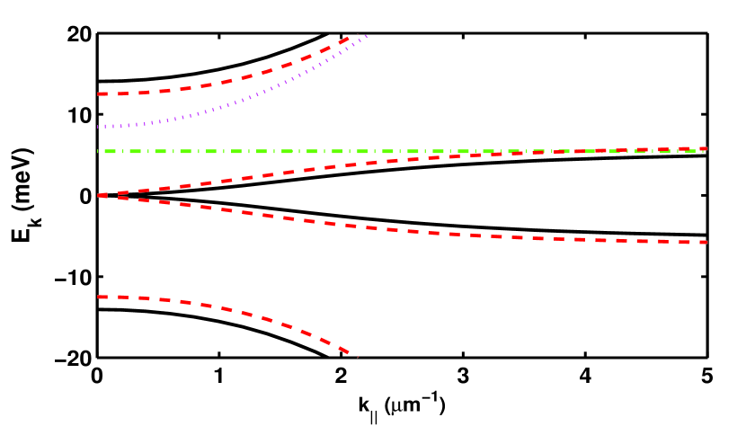
Figure 1: The dispersion of the normal modes of the system for polariton density $n_{p}=5\mu\mbox{m}^{-2}$ (solid) and $n_{p}=50\mu\mbox{m}^{-2}$ (dashed). The uncoupled photon (dotted) and exciton (dash-dotted) modes are also shown.

The modification of the energy splitting between the lower and the upper polariton branch is accurately characterized in Fig. 2, where the energy shifts of the two polariton modes at ${\bf k}=0$ are plotted as a function of the density. Exciton saturation and interactions result in a global blue-shift of the lower polariton and a red-shift of the upper polariton. The shifts are linear as a function of the density, but their slope varies close to threshold. As highlighted in the inset, the slope of the lower polariton shift changes by a factor of two across the threshold, because the contribution of the condensed populations ($n^{0}_{xx}$, $n^{0}_{xc}$) is one half the contribution of the thermal populations ($\tilde{n}_{xx}$, $\tilde{n}_{xc}$), as seen in Eq. (15).

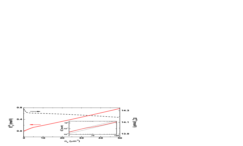
Figure 2: Lower (solid) and upper (dashed) polariton energies at $k=0$ vs polariton density $n_{p}$. Inset: Double logarithmic plot of the lower polariton energy. The thin dotted lines highlight the two different slopes below and above the density threshold.

We now turn to the thermodynamic properties of the system. In Fig. 3(a), we report the density-temperature BEC phase diagram, as computed for $A=1000~{}\mu\mbox{m}^{2}$. The phase boundary in the calculations has been set by the occurrence of a finite fraction of polariton condensate larger than $1\%$. In the plot, a few values of the quantity $|X_{0}|^{2}$ along the phase boundary are indicated. This quantity represents the exciton amount in the polariton condensate. It decreases for increasing density, depending on the exciton saturation and the change in detuning. For very large densities this quantity eventually vanishes, corresponding to the crossover to a photon-laser regime. However, for the studied GaAs model microcavity, the variation of the exciton amount in the condensate field remains very small up to densities far above the experimentally estimated polariton density Deng et al. (2006, 2003). This is basically due to the positive cavity detuning, sufficiently large to be robust to the exciton nonlinear energy shift. On the other hand, due to the same feature and to the flat energy dispersion of the exciton-like lower polariton states, a large population can be accommodated in the excited state when the temperature exceeds $25$ K, thus dramatically increasing the BEC transition density, eventually leading to the direct occurrence of photon-lasing. In particular, for this system, we predict that equilibrium polariton BEC is impossible for temperatures larger than $30$ K. In Fig. 3(b), we show a detail of the low-$T$ region of the phase diagram, computed for two different system areas $A=100~{}\mu\mbox{m}^{2}$ and $A=1000~{}\mu\mbox{m}^{2}$. In a homogeneous two-dimensional system, in the limit of infinite size, a true condensate cannot exist due to the divergence of low-energy thermal fluctuations. The transition to a superfluid state is instead expected, giving rise to the Berezinski-Kosterlitz-Thouless crossover with spontaneous unbinding of vortices. The divergence of the condensate fluctuations has however a logarithmic dependence on the system size. Fig. 3(b) shows this behaviour as a slow increase of the critical density for increasing $A$. Quantitatively, the critical density varies by no more than a factor 2 at $T=1$ K, for the two considered values of the system area. This difference becomes even smaller for larger temperatures. The predicted dependence on the system size could be experimentally verified only in samples with improved interface quality and manifesting thermalization at very low polariton temperature Sarchi and Savona (2007b).

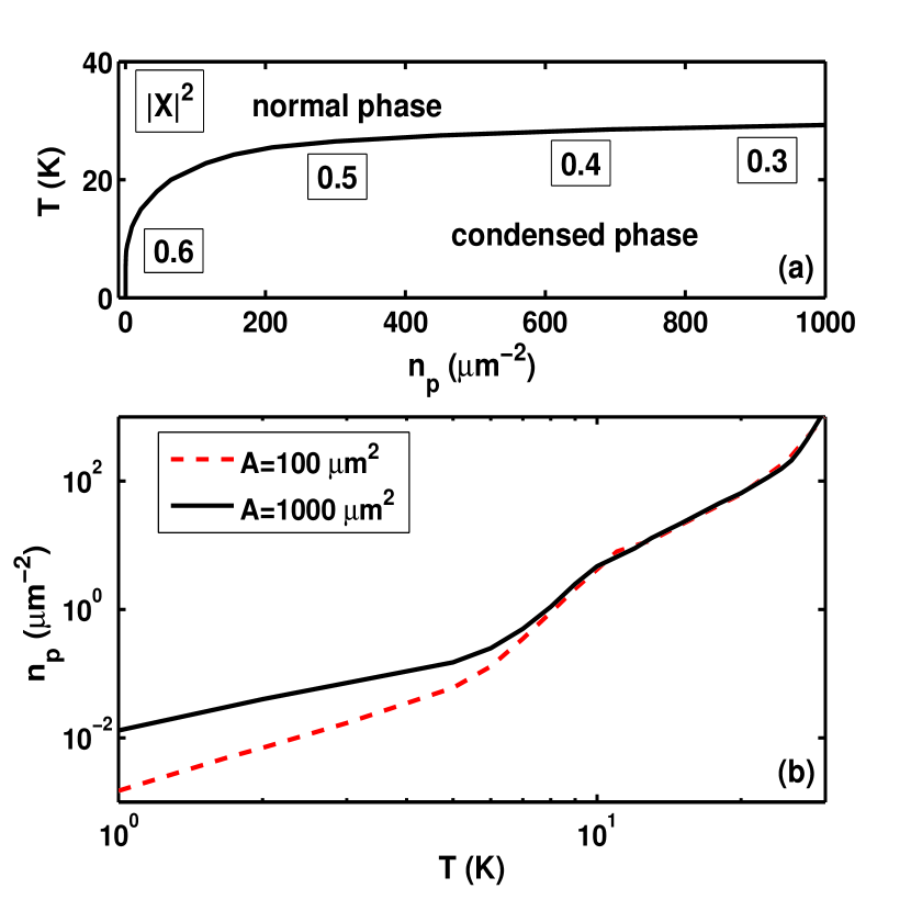
Figure 3: (a) Phase diagram of the polariton condensation, computed for $A=1000~{}\mu\mbox{m}^{2}$. The exciton fraction in the condensate $|X_{0}|^{2}$, along the phase boundary, is indicated in boxes. (b) Detail of the low-$T$ region where we also display the transition boundary computed for $A=100~{}\mu\mbox{m}^{2}$.

IV Linear response in the HFP limit

Within the present theory, it is easy to compute the density fluctuation of the exciton or the photon field produced by a perturbation acting on either of them. This quantity is particularly interesting because as we suggest later, it might be used to study the nature of the polariton condensate via fully optical or mechanical perturbations.

We consider the time dependent perturbation

$$\hat{H}_{pert}(t)=\int d{\bf r}\hat{n}^{\chi\chi}({\bf r},t)V_{ext}({\bf r},t)\,,$$ (37)

driven by the external potential $V_{ext}({\bf r},t)$ affecting the field $\hat{\Psi}_{\chi}({\bf r},t)$ ($\chi=x,c$). This perturbation results in a density fluctuation

$$\delta n^{\xi\xi}({\bf r},t)\equiv n^{\xi\xi}({\bf r},t)-n_{eq}^{\xi\xi}({\bf r},t)\,,$$ (38)

($\xi=x,c$) around the equilibrium value $n^{eq}_{\xi\xi}({\bf r},t)$. Within the linear response limit, this fluctuation is given by Pitaevskii and Stringari (2003); Fetter and Walecka (1971)

$$\delta n^{\xi\chi}({\bf r},t)=\frac{i}{\hbar}\int_{-\infty}^{t}dt^{\prime}\int d{\bf r^{\prime}}C_{\xi\chi}({\bf r^{\prime}},t^{\prime};{\bf r},t)V_{ext}({\bf r^{\prime}},t^{\prime})\,,$$ (39)

where

$$C_{\xi\chi}({\bf r^{\prime}},t^{\prime};{\bf r},t)=\langle\left[\hat{n}^{\chi\chi}({\bf r^{\prime}},t^{\prime}),\hat{n}^{\xi\xi}({\bf r},t)\right]\rangle\,.$$ (40)

For a spatially uniform system in steady state, the density commutator Eq. (40) only depends on ${\bf r-r^{\prime}}$ and $t-t^{\prime}$. Then, by Fourier transforming Eq. (39), we get the expression

$$\delta n^{\xi\chi}({\bf k},\omega)=D^{r}_{\xi\chi}({\bf k},\omega)V_{ext}({\bf k},\omega)\,,$$ (41)

where

$$D^{r}_{\xi\chi}({\bf k},\omega)=-\frac{1}{\hbar}\int\frac{d\omega^{\prime}}{2\pi}\frac{C_{\xi\chi}({\bf k},\omega-\omega^{\prime})}{\omega^{\prime}+i0^{+}}$$ (42)

is the retarded density-density correlation Fetter and Walecka (1971), and $C_{\xi\chi}({\bf k},\omega)$ is the Fourier transform of $C_{\xi\chi}({\bf r},t)$.

Using the framework developed in Section II, we write the real-time density operators $\hat{n}^{\chi\chi}({\bf r},t)$ in the polariton basis, via Eqs. (1-2) and by inverting the transformation Eq. (31)

$$\hat{O}_{\chi}({\bf k},t)=\sum_{j=lp,up}\Pi^{j}_{\chi}({\bf k})e^{-i\frac{E_{\bf k}^{j}}{\hbar}t}\hat{\pi}^{j}_{\bf k}+\Upsilon^{j}_{\chi}({\bf k})e^{i\frac{E_{\bf k}^{j}}{\hbar}t}\hat{\pi}^{j\dagger}_{-\bf k}\,.$$ (43)

Here, the factors $\Pi^{j}_{\chi}({\bf k})$ and $\Upsilon^{j}_{\chi}({\bf k})$ define the components of the exciton (photon) field on the forward and backward propagating lower and upper polariton eigenmodes. Within the HFP limit, the density commutator consists of three contributions Minguzzi and Tosi (1997)

$$C_{\xi\chi}({\bf r},t) = {}^{0}C_{\xi\chi}^{I}({\bf r},t)+^{0}C_{\xi\chi}^{II}({\bf r},t)+\tilde{C}_{\xi\chi}({\bf r},t)$$

$$= \left(\Phi^{*}_{\xi}(0)\Phi_{\chi}(t)\langle\left[\tilde{\psi}_{\xi}({\bf 0},0),\tilde{\psi}_{\chi}^{\dagger}({\bf r},t)\right]\rangle-h.c.\right)$$

$$+ \left(\Phi^{*}_{\xi}(0)\Phi^{*}_{\chi}(t)\langle\left[\tilde{\psi}_{\xi}({\bf 0},0),\tilde{\psi}_{\chi}({\bf r},t)\right]\rangle-h.c.\right)$$

$$+ \langle\left[\tilde{\psi}^{\dagger}_{\xi}({\bf 0},0)\tilde{\psi}_{\xi}({\bf 0},0),\tilde{\psi}_{\chi}^{\dagger}({\bf r},t)\tilde{\psi}_{\chi}({\bf r},t)\right]\rangle\,,$$

the first two terms arising from the presence of the condensate fields. Correspondingly, the retarded density-density correlation can be written as the sum of three terms

$$D^{r}_{\xi\chi}({\bf k},\omega)=\hskip 1.42271pt^{0}D^{I}_{\xi\chi}({\bf k},\omega)+\hskip 1.42271pt^{0}D^{II}_{\xi\chi}({\bf k},\omega)+\tilde{D}_{\xi\chi}({\bf k},\omega)\,.$$ (45)

The first two terms survive only in the presence of a condensate while the third one only depends on the thermal population (however it is affected by the modification of the one-particle spectrum induced by the condensate). In detail, the first term describes the excitation of particles out of the condensate and it is given by

$${}^{0}D^{I}_{\xi\chi}({\bf k},\omega)=\sum_{j=lp,up}\left[N^{j}_{\xi\chi}({\bf k},\omega)+N^{j}_{\xi\chi}({\bf k},-\omega)^{*}\right]\,,$$ (46)

with

$$N^{j}_{\xi\chi}({\bf k},\omega)=\frac{\Phi_{\xi}\Phi^{*}_{\chi}\Pi_{\xi}^{j*}({\bf k})\Pi_{\chi}^{j}({\bf k})+\Phi_{\xi}^{*}\Phi_{\chi}\Upsilon_{\xi}^{j*}({\bf k})\Upsilon_{\chi}^{j}({\bf k})}{\hbar\omega-E_{\bf k}^{j}+i0^{+}}\,.$$ (47)

The second term describes the de-excitation of the thermal population into the condensate and it is given by

$${}^{0}D^{II}_{\xi\chi}({\bf k},\omega)=\sum_{j=lp,up}\left[A^{j}_{\xi\chi}({\bf k},\omega)+A^{j}_{\xi\chi}({\bf k},-\omega)^{*}\right]\,,$$ (48)

with

$$A^{j}_{\xi\chi}({\bf k},\omega)=\frac{\Phi_{\xi}\Phi_{\chi}\Pi_{\xi}^{j*}({\bf k})\Upsilon^{j}_{\chi}({\bf k})+\Phi_{\xi}^{*}\Phi^{*}_{\chi}\Upsilon_{\xi}^{j*}({\bf k})\Pi^{j}_{\chi}({\bf k})}{\hbar\omega-E_{\bf k}^{j}+i0^{+}}\,.$$ (49)

The third term describes the oscillations of the thermal population and it is given by

$$\tilde{D}_{\xi\chi}({\bf k},\omega)=\sum_{j=lp,up}\left[T^{j}_{\xi\chi}({\bf k},\omega)+T^{j}_{\xi\chi}({\bf k},-\omega)^{*}\right]\,,$$ (50)

with

$$T^{j}_{\xi\chi}({\bf k},\omega) = \sum_{l,{\bf q}}\left[\frac{F^{jl}_{\xi\chi}({\bf k,q})\left(\bar{N}^{l}_{\bf q}-\bar{N}^{j}_{\bf q-k}\right)}{\hbar\omega+E_{\bf q-k}^{j}-E_{\bf q}^{l}+i0^{+}}\right.$$ (51)

$$+\left.\frac{R^{jl}_{\xi\chi}({\bf k,q})\left(1+\bar{N}^{l}_{\bf q}+\bar{N}^{j}_{\bf q-k}\right)}{\hbar\omega+E_{\bf q-k}^{j}+E_{\bf q}^{l}+i0^{+}}\right]\,$$

and

$$F^{jl}_{\xi\chi}({\bf k,q}) = \Pi^{j}_{\xi}({\bf q-k})\Pi_{\chi}^{j*}({\bf q-k})\Pi_{\xi}^{l*}({\bf q})\Pi_{\chi}^{l}({\bf q})$$ (52)

$$+ \Pi_{\xi}^{j}({\bf q-k})\Upsilon_{\chi}^{j*}({\bf q-k})\Pi_{\xi}^{l*}({\bf q})\Upsilon_{\chi}^{l}({\bf q})\,,$$

$$R^{jl}_{\xi\chi}({\bf k,q}) = \Pi^{j}_{\xi}({\bf q-k})\Pi_{\chi}^{j*}({\bf q-k})\Upsilon_{\xi}^{l}({\bf q})\Upsilon_{\chi}^{l*}({\bf q})$$ (53)

$$+ \Pi_{\xi}^{j}({\bf q-k})\Upsilon_{\chi}^{j*}({\bf q-k})\Upsilon_{\xi}^{l}({\bf q})\Pi_{\chi}^{l*}({\bf q})\,.$$

We use these equations to study the fluctuation $\delta n_{cc}$ of the photon density, directly related to the photoluminescence measured in experiments, produced by an optical (affecting the photon field) or mechanical (affecting the exciton field) perturbation. We take, as external potential, a plane wave with wave vector ${\bf k_{ext}}$, delta-pulsed in time, i.e. $V_{ext}({\bf r},t)=V_{0}e^{i{\bf k}_{ext}\cdot{\bf r}}\delta(t-t_{0})$. In this case, from Eq. (41), we see that $\delta n^{\xi\chi}({\bf k},\omega)=V_{0}D^{r}_{\xi\chi}({\bf k},\omega)\delta({\bf k-k}_{ext})$, i.e. the response is diagonal in ${\bf k}$ and is simply proportional to the correlation $D^{r}$. The imaginary part of $D^{r}$ describes the energy transfer to the system and thus it is the most relevant function.

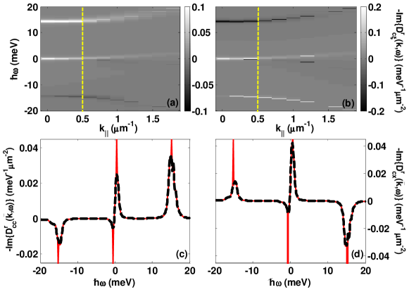
Figure 4: Imaginary part of the retarded density-density correlations $D^{r}_{cc}({\bf k},\omega)$ (panel a and c) and $D^{r}_{cx}({\bf k},\omega)$ (b and d), as computed for $T=10$ K and $n_{p}=5~{}\mu\mbox{m}^{-2}$. In panels (a) and (b) we display the $k-\omega$ dependence of the correlation in grey tones. In panels (c) and (d) the same quantities are plotted as a function of the energy $\hbar\omega$ and at the wave vector $\bar{k}=0.5~{}\mu\mbox{m}^{-1}$. In panels (c)-(d), the dashed line represents the contribution $\tilde{D}^{r}_{\xi\chi}({\bf k},\omega)$ arising from the oscillations of the non condensate. Delta peaks arise from the oscillation of the condensate. At high energy (i.e. at the upper polariton energy), the photon-photon response corresponds to absorption at positive energy and gain at negative energy, while the photon-exciton response has the opposite behavior.

The resulting quantities $-\mbox{Im}\{D^{r}_{c\chi}({\bf k},\omega)\}$ with $\chi=c,x$ are shown in Fig. 4. We display the results for the photon-photon (panels (a)-(c)) and photon-exciton (panels (b)-(d)) correlation in the condensed regime. Poles at negative energy are present for both quantities, due to the spectrum modification induced by condensation. While the condensate contribution defines collective modes with infinite lifetime (delta-peaks), the contribution from the thermal population is responsible for a finite linewidth, as can be argued from the equations above. The surprising result of this analysis is however the unusual behavior manifested by the photon-exciton response at high energy. In this case, the collective mode corresponds to gain at positive energy and to absorption at negative energy. Conversely, for the photon-photon response, we expect to observe the opposite behavior. This feature is due to the phases of the Hopfield coefficients. As shown by Eqs. (47,49), the opposite nature of the collective modes generated by optical or mechanical perturbations would be observed in experiments only if an exciton coherent field $\Phi_{x}$ is present. Furthermore, the relative amplitude of the two responses is proportional to the fraction of coherence of each field, giving direct access to the amount of exciton condensate. In this respect, we point out that, although any kind of perturbation would affect simultaneously both the exciton and the photon field de Lima Jr. et al. (2006), the geometry of the system can be chosen in such a way that the effect of the perturbation on one of the two fields be dominant (see for example the static perturbation affecting the exciton field used by Balili et al. Balili et al. (2007)). We thus suggest that an ideal tool to observe these features, would be a pump and probe experiment where the probe be in turn optical or mechanical (for example produced by a coherent acoustic waves de Lima Jr. et al. (2006)).

V Conclusions

We generalized the HFP theory to the case of two coupled Bose fields at equilibrium. The theory allows modeling the BEC of microcavity polaritons in very close analogy with the BEC of a weakly interacting gas Fetter and Walecka (1971); Pitaevskii and Stringari (2003). In particular we treat simultaneously both the linear exciton-photon coupling and interactions. We account for the presence of a non condensed population as well. Within this description we are able to predict the modification of the spectrum and the thermodynamic properties for increasing density. Since the theory allows to describe simultaneously the properties of the polariton, the photon and the exciton fields, it allows the understanding of typical optical measurements. In particular, our analysis supports the interpretation of the recent experimental findings Kasprzak et al. (2006); Balili et al. (2007); Deng et al. (2006) in terms of BEC of a trapped gas. We have applied the theory to compute the density-density response of a polariton gas to an external perturbation. This quantity can be characterized in pump and probe experiments realized with an optical or mechanical probe. In particular, we predict that the upper polariton energy collective modes generated in the two cases have a response of opposite sign. We suggest that the observation of this feature would be a proof of the presence of an exciton condensate and would answer the long standing question about the connection between polariton BEC and a laser phenomenon.

We acknowledge financial support from the Swiss National Foundation through project N. PP002-110640.

References

• Kasprzak et al. (2006) J. Kasprzak, M. Richard, S. Kundermann, A. Baas, P. Jeambrun, J. M. J. Keeling, F. M. Marchetti, M. H. Szymaska, R. André, J. L. Staehli, et al., Nature 443, 409 (2006).
• Balili et al. (2007) R. Balili, V. Hartwell, D. Snoke, L. Pfeiffer, and K. West, Science 316, 1007 (2007), eprint http://www.sciencemag.org/cgi/reprint/316/5827/1007.pdf, URL http://www.sciencemag.org/cgi/content/abstract/316/5827/1007.
• Deng et al. (2006) H. Deng, D. Press, S. Gotzinger, G. S. Solomon, R. Hey, K. H. Ploog, and Y. Yamamoto, Phys. Rev. Lett. 97, 146402 (pages 4) (2006), URL http://link.aps.org/abstract/PRL/v97/e146402.
• Laussy et al. (2004) F. P. Laussy, G. Malpuech, A. Kavokin, and P. Bigenwald, Phys. Rev. Lett. 93, 016402 (pages 4) (2004), URL http://link.aps.org/abstract/PRL/v93/e016402.
• Schwendimann and Quattropani (2006) P. Schwendimann and A. Quattropani, Phys. Rev. B 74, 045324 (pages 10) (2006), URL http://link.aps.org/abstract/PRB/v74/e045324.
• Keeling et al. (2004) J. Keeling, P. R. Eastham, M. H. Szymanska, and P. B. Littlewood, Phys. Rev. Lett. 93, 226403 (pages 4) (2004), URL http://link.aps.org/abstract/PRL/v93/e226403.
• Marchetti et al. (2006) F. M. Marchetti, J. Keeling, M. H. Szymanska, and P. B. Littlewood, Phys. Rev. Lett. 96, 066405 (2006).
• Szymanska et al. (2006) M. H. Szymanska, J. Keeling, and P. B. Littlewood, Phys. Rev. Lett. 96, 230602 (pages 4) (2006), URL http://link.aps.org/abstract/PRL/v96/e230602.
• Doan et al. (2005) T. D. Doan, H. T. Cao, D. B. T. Thoai, and H. Haug, Phys. Rev. B 72, 085301 (pages 7) (2005), URL http://link.aps.org/abstract/PRB/v72/e085301.
• Sarchi and Savona (2006) D. Sarchi and V. Savona, phys. stat. sol. (b) 243, 2317 (2006).
• Wouters and Carusotto (2007) M. Wouters and I. Carusotto, ArXiv:cond-mat/0702431 (2007).
• Sarchi and Savona (2007a) D. Sarchi and V. Savona, Phys. Rev. B 75, 115326 (2007a).
• Savona and Tassone (1995) V. Savona and F. Tassone, Solid State Comm. p. 673 (1995).
• Savona et al. (1999) V. Savona, C. Piermarocchi, A. Quattropani, P. Schwendimann, and F. Tassone, Phase Transitions 68, 169 (1999).
• Laikhtman (2007) B. Laikhtman, J. Phys.: Cond. Matter 19, 295214 (2007).
• Shi and Griffin (1998) H. Shi and A. Griffin, Phys. Rep. 304, 1 (1998).
• Pitaevskii and Stringari (2003) L. Pitaevskii and S. Stringari, Bose-Einstein condensation (Clarendon Oxford University Press, Oxford, 2003).
• Langbein and Hvam (2002) W. Langbein and J. M. Hvam, Phys. Rev. Lett. 88, 047401 (2002), URL http://link.aps.org/abstract/PRL/v88/e047401.
• Richard et al. (2005a) M. Richard, J. Kasprzak, R. Andre, R. Romestain, L. S. Dang, G. Malpuech, and A. Kavokin, Phys. Rev. B 72, 201301 (2005a), URL http://link.aps.org/abstract/PRB/v72/e201301.
• Deng et al. (2003) H. Deng, G. Weihs, D. Snoke, J. Bloch, and Y. Yamamoto, PNAS 100, 15318 (2003).
• Richard et al. (2005b) M. Richard, J. Kasprzak, R. Romestain, R. Andre, and L. S. Dang, Phys. Rev. Lett. 94, 187401 (2005b), URL http://link.aps.org/abstract/PRL/v94/e187401.
• Hohenberg (1967) P. C. Hohenberg, Phys. Rev. 158, 383 (1967).
• Lauwers et al. (2003) J. Lauwers, A. Verbeure, and V. A. Zagrebnov, J. Phys. A 36, L169 (2003).
• Schmitt-Rink et al. (1985) S. Schmitt-Rink, D. S. Chemla, and D. A. B. Miller, Phys. Rev. B 32, 6601 (1985).
• Rochat et al. (2000) G. Rochat, C. Ciuti, V. Savona, C. Piermarocchi, A. Quattropani, and P. Schwendimann, Phys. Rev. B 61, 13856 (2000).
• Okumura and Ogawa (2001) S. Okumura and T. Ogawa, Phys. Rev. B 65, 035105 (2001).
• Fetter and Walecka (1971) A. L. Fetter and J. D. Walecka, Quantum Theory of Many-Particle Systems (McGraw-Hill, 1971).
• Sarchi and Savona (2007b) D. Sarchi and V. Savona, Solid State Comm., in press, doi:10.1016/j.ssc.2007.07.039 (2007b).
• Minguzzi and Tosi (1997) A. Minguzzi and M. P. Tosi, J. Phys.: Cond. Matter 9, 10211 (1997).
• de Lima Jr. et al. (2006) M. M. de Lima Jr., M. van der Poel, P. V. Santos, and J. M. Hvam, Phys. Rev. Lett. 97, 045501 (2006), URL http://link.aps.org/abstract/PRL/v97/e045501.
• Shelykh et al. (2006) I. A. Shelykh, Y. G. Rubo, G. Malpuech, D. D. Solnyshkov, and A. Kavokin, Phys. Rev. Lett. 97, 066402 (pages 4) (2006), URL http://link.aps.org/abstract/PRL/v97/e066402.
• Liu et al. (2004) X.-J. Liu, H. Hu, A. Minguzzi, and M. P. Tosi, Phys. Rev. A 69, 043605 (pages 11) (2004), URL http://link.aps.org/abstract/PRA/v69/e043605.