The Order of Phase Transitions in Barrier Crossing

Abstract

A spatially extended classical system with metastable states subject to weak spatiotemporal noise can exhibit a transition in its activation behavior when one or more external parameters are varied. Depending on the potential, the transition can be first or second-order, but there exists no systematic theory of the relation between the order of the transition and the shape of the potential barrier. In this paper, we address that question in detail for a general class of systems whose order parameter is describable by a classical field that can vary both in space and time, and whose zero-noise dynamics are governed by a smooth polynomial potential. We show that a quartic potential barrier can only have second-order transitions, confirming an earlier conjecture Stein (2004). We then derive, through a combination of analytical and numerical arguments, both necessary conditions and sufficient conditions to have a first-order vs. a second-order transition in noise-induced activation behavior, for a large class of systems with smooth polynomial potentials of arbitrary order. We find in particular that the order of the transition is especially sensitive to the potential behavior near the top of the barrier.

I Introduction

When a spatially extended classical system with multiple locally stable states is perturbed by weak spatiotemporal noise, a transition in its activation behavior can occur as one or more parameters of the system are varied Maier and Stein (2001, 2003); Stein (2004). In the simplest one-dimensional systems this parameter is simply the length of the interval on which the system is defined, but for more complicated systems other parameters come into play. For example, a transition from Arrhenius to non-Arrhenius behavior in thermally activated magnetization reversal in thin annular nanomagnets can occur either as ring size increases or as the externally applied magnetic field decreases Martens et al. (2005, 2006). Another example is a crossover from uniform to instanton-like decay of metastable metal nanowires Bürki et al. (2005) as either the length of the nanowire or the stress applied to it is varied. A similar crossover, from thermal activation to quantum tunneling, occurs in various systems as temperature is lowered  Goldanskii (1959); Affleck (1981); Wolynes (1981); Caldeira and Leggett (1981); Larkin and Ovchinnikov (1983); Grabert and Weiss (1984); Riseborough et al. (1985); Chudnovsky (1992); Kondo and Takayanagi (1997); Gorokhov and Blatter (1997); Frost and Yaffe (1999).

These two cases are formally related through a mapping that identifies interval length (and/or magnetic field, stress, if appropriate) in the classical field case to temperature in the quantum case; in particular, increasing interval length in the former corresponds to the lowering of temperature in the latter, with thermal activation in a classical field theory of infinite domain size mapping to zero-temperature tunneling in quantum field theories. These transitions are fundamentally different from the more usual sort, in which a change in order parameter (i.e., expectation value of the field) results from varying a control parameter, such as coupling strengths in the Hamiltonian or noise amplitude. (For an extensive discussion of this more conventional kind of transition within a noisy field-theoretical framework, see, for example, Buceta and Lindenberg (2004).) The extent to which the more unconventional type of transition under discussion here can be compared to a true second-order phase transition, and where the analogy breaks down, was discussed extensively in Stein (2005). (For recent work on discretized versions of these and similar models, see Berglund et al. (2007a, b).)

Chudnovsky Chudnovsky (1992) first noted that the classical$\leftrightarrow$quantum transition in an extended system with a single degree of freedom can be either first- or second-order, depending on the potential. This observation has important applications. First-order transitions in the classical-quantum escape rate have been considered in anisotropic bistable large-spin models Chudnovsky and Garanin (1997) and biaxial spin systems subject to longitudinal fields Garanin and Chudnovsky (1999), and have been more generally considered in the decay of metastable states in quantum field theories Kuznetsov and Tinyakov (1997); Gorokhov and Blatter (1997). A general discussion can be found in Chudnovsky and Tejada (1998).

Similarly, a first-order transition can also occur in classical transitions between two thermally activated regimes, as was recently found by the authors Bürki et al. (2005) in the decay of nanowires due to thermal fluctuations (cf. Fig. 2 of Ref. Bürki et al. (2005)). Despite its potential importance, relatively little systematic work has been done to identify the general conditions under which one or the other kind of transition occurs. It was conjectured Stein (2004) that smooth polynomial potentials with terms no higher than quartic display only second-order transitions. It is also known that higher-order terms can lead to a first-order transition  Kuznetsov and Tinyakov (1997). At the present time, however, there is no systematic theory of how the order of the transition depends on potential characteristics. The purpose of this paper is to address that problem.

II Model

We will consider a general class of models of extended systems describable by a classical field $\phi(z,t)$ defined on the spatial interval $[-L/2,L/2]$, subject to a potential $V(\phi)$ and perturbed by spatiotemporal white noise not . Time evolution is governed by the stochastic Ginzburg-Landau equation

$$\partial_{t}\phi=\partial_{zz}\phi-\partial_{\phi}V(\phi)+\sqrt{2T}\xi(z,t)\,,$$ (1)

where all dimensional quantities have been scaled out. The first term on the RHS arises from a field ‘stiffness’, i.e., an energy penalty for spatial variations of the field. The noise $\xi(z,t)$ satisfies $\langle\xi(z_{1},t_{1})\xi(z_{2},t_{2})\rangle=\delta(z_{1}-z_{2})\delta(t_{1}-t_{2})$, and its magnitude $T$ is small compared to all other energy scales in the problem (formally, our analysis will be asymptotically valid in the $T\to 0$ limit).

The zero-noise dynamics of (1) can be written as the variation of an action ${\cal H}$ with the field $\phi$:

$$\partial_{t}\phi=-\delta{\cal H}/\delta\phi$$ (2)

with

$${\cal H}[\phi]\equiv\int_{-L/2}^{L/2}dz\ \left[\frac{1}{2}(\partial_{z}\phi)^{2}+V(\phi)\right]\,.$$ (3)

Stationary solutions of (2) describe stable, metastable, and transition (i.e., saddle) states of the system.

In the weak-noise ($T\to 0$) limit, the classical activation rate for a transition out of a (meta)stable well is

$$\Gamma\sim\Gamma_{0}\exp(-\Delta W/T)\,,$$ (4)

where the activation barrier $\Delta W$ is the action difference between the transition state and the initial (meta)stable state. The rate prefactor $\Gamma_{0}$ is determined by fluctuations about the most probable escape path. When the top of the barrier is locally quadratic, the prefactor $\Gamma_{0}$ is independent of temperature. In such circumstances the escape rate (4) is said to be of the Arrhenius-van’t Hoff (or often simply Arrhenius) form. Here we will mostly be concerned with the behavior of the activation barrier $\Delta W$.

III Transition in activation behavior

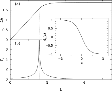
Figure 1: (a) The activation energy $\Delta W$ and (b) the rate prefactor $\Gamma_{0}$ as functions of the interval length $L$, for the potential given by Eq. (5) with Neumann boundary conditions. The dashed line indicates the critical interval length $L_{c}=\pi/2$ at which the saddle state bifurcation takes place, showing the power-law divergence of the prefactor. The transition state $\phi_{t}(z)$ for $L=5$ (corresponding to $m=0.986$) described by Eq. (6) is displayed in the inset (only one of the symmetric pair is shown.) Note that quantities in all figures are expressed in dimensionless units (see text.)

We briefly summarize here the derivation of a second-order transition in the noise-induced barrier crossing described by (1) between wells in the simple bistable symmetric quartic potential

$$V_{s}(\phi)=(\phi^{2}-1)^{2},$$ (5)

with Neumann boundary conditions $\partial_{z}\phi|_{-L/2}=\partial_{z}\phi|_{L/2}=0$. The discussion follows that of Stein (2005), to which we refer the reader for details.

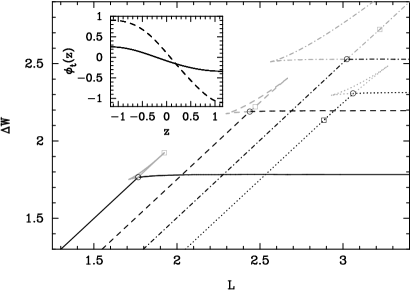
Figure 2: Activation barrier $\Delta W$ (black lines) for various potentials exhibiting first-order transitions, marked by open circles. The line styles correspond to the following potentials: (solid) $V(\phi)=1-4\phi^{2}/3-\phi^{4}+4\phi^{5}/3$, (dashed) $V(\phi)=1-\phi^{2}-\phi^{3}+\phi^{5}$, (dot-dashed) $V(\phi)=1-2\phi^{2}/3-3\phi^{3}/2+7\phi^{5}/6$, and (dotted) $V(\phi)=1-13\phi^{2}/12-\phi^{3}+\phi^{4}/4+5\phi^{5}/6$, with the curves shifted horizontally to improve readability. The (second-order) transition between uniform and instanton-type escape is marked by an open square for each curve. Activation barriers for higher energy states are shown with gray lines. Degenerate instanton-like saddle states corresponding to the first-order transition for the dotted line are shown in the inset. Both states have the same length and energy. Note that the potential described by the rightmost curve (dotted line) exhibits a second-order followed by a first-order transition.

Because of the symmetry of the potential (which is not necessary for the transition to occur Stein (2004)), the change in activation behavior arises from a bifurcation of the transition state. Below a critical length $L_{c}$ the transition state $\phi_{t}$ is constant, while above $L_{c}$ it becomes a pair of degenerate, spatially varying instanton configurations Maier and Stein (2001):

$$\phi_{t}=\begin{cases}0,&L<L_{c}\\ \pm\sqrt{\frac{2m}{1+m}}{\rm sn}({\frac{2z}{\sqrt{m+1}}}\mid m),\qquad&L\geq L_{c}\end{cases}$$ (6)

where ${\rm sn}(\cdot\mid m)$ is the Jacobi elliptic $\rm sn$ function with parameter $0\leq m\leq 1$. Its quarter-period is given by ${\bf K}(m)$, the complete elliptic integral of the first kind Abramowitz and Stegun (1965), which is a monotonically increasing function of $m$. As $m\to 0^{+}$, ${\bf K}(m)$ decreases to $\pi/2$, and ${\rm sn}(\cdot\mid m)\to\sin(\cdot)$. In this limit the saddle state smoothly degenerates to the $\phi_{t}=0$ configuration. As $m\to 1^{-}$, the quarter-period increases to infinity (with a logarithmic divergence), and ${\rm sn}(\cdot\mid m)\to\tanh(\cdot)$, the (nonperiodic) single-kink sigmoidal function. The Langer-Callan-Coleman Langer (1967, 1969); Coleman (1977); Callan and Coleman (1977) ‘bounce’ solution is thereby recovered as $L\to\infty$.

The value of $m$ in (6) is determined by the interval length $L$ and the Neumann boundary conditions, which require that

$$L=\sqrt{m+1}\,{\bf K}(m)\,$$ (7)

The critical length is determined by (7) when $m=0$; that is, $L_{c}=\pi/2$. As previously noted, $m\to 1$ corresponds to $L\to\infty$, and the activation energy smoothly approaches the asymptotic value of $\Delta W_{\infty}=4\sqrt{2}/3$. The transition state for an intermediate value of $m$, corresponding to $L=5$, is shown in the inset of Fig. 1.

The activation energy $\Delta W$ can be computed in closed form for all $L>L_{c}$ (below $L_{c}$, it is simply $\Delta W=L$):

$$\Delta W=\frac{8(1+m){\bf E}(m)-(1-m)(3m+5){\bf K}(m)}{3(1+m)^{3/2}},$$ (8)

with ${\bf E}(m)$ the complete elliptic integral of the second kind Abramowitz and Stegun (1965). The activation energy as a function of $L$ is shown in Fig. 1(a). Note that the curve of $\Delta W$ vs. $L$ and its first derivative are both continuous at $L_{c}$; the second derivative, however, is discontinuous, as might be expected of a second-order-like phase transition.

A more profound manifestation of critical behavior at $L_{c}$ is exhibited by the rate prefactor $\Gamma_{0}$, which (in the asymptotic limit $T\to 0$) diverges at $L_{c}$, as shown in Fig. 1(b). This is striking, but requires interpretation. Because it is not relevant to the present discussion, we refer the interested reader to Stein (2005).

This behavior is generic for a whole class of potentials, as described below, but first-order transitions have also been observed Bürki et al. (2005), leading to a continuous but non-differentiable activation barrier $\Delta W$ at the transition points. This is illustrated for various potentials in Fig. 2. The second-order transition is still present, but is usually not physically observable, as it happens for higher energy transition states (note, however, the exception in Fig. 2, dotted line).

IV Order of the transition

Figure 3: The energy of the classical trajectory determining activation behavior for (solid line) the symmetric quartic potential of Eq. (5), (dashed line) $V(\phi)=1-5\phi^{2}/2+\phi^{3}+\phi^{4}/2$, (dot-dashed line) $V(\phi)=1-2\phi^{2}+\phi^{3}/2+\phi^{5}/2$, and (dotted line) $V(\phi)=1-7\phi^{2}/4+\phi^{3}/3+5\phi^{6}/12$. The corresponding potentials $V(\phi)$ are plotted in the inset. As discussed in the text, the monotonic decrease of energy with interval length signifies a second-order phase transition at $L_{c}$.

Eqs. (2) and (3) lead to the (typically nonlinear) differential equation for stationary states

$$\phi^{\prime\prime}=V^{\prime}(\phi).$$ (9)

If we map the field $\phi$ to position and the coordinate $z$ to time, the solutions to this equation are equivalent to the trajectories of a classical particle moving in the inverted potential $-V(\phi)$ Hänggi et al. (1990). The bounce, or ‘instanton’, transition state (cf. Eq. (6) that determines the activation behavior when $L>L_{c}$) then corresponds to a half-period of such a periodic classical trajectory.

Figure 4: The energy of the classical trajectory determining activation behavior for various potentials exhibiting first-order transitions, as evidenced by the non-monotonic behavior of $L(E)$. The line styles correspond to those of Fig. 2, with the corresponding potentials $V(\phi)$ plotted in the inset.

These classical trajectories have a corresponding “energy” $\tilde{E}\equiv-E(L)$ given by (cf. Eq. (6) of Chudnovsky (1992))

$$-E(L)=\frac{1}{2}(\phi^{\prime})^{2}-V(\phi)\,.$$ (10)

This energy of a classical instanton trajectory should not be confused with the activation barrier $\Delta W$ given by the action difference between the transition and metastable states. $\tilde{E}$ corresponds to the energy of a classical particle undergoing periodic motion in the inverted potential $-V(\phi)$. It is determined either by the temperature in the thermally assisted tunneling problem, or by the interval length in a stochastic classical Ginzburg-Landau field theory.

Figure 5: (Color online) Various types of potentials of the form given by Eq. (12), with the second term $\alpha\phi^{m}/m$ plotted as a (blue) dashed line, and the other terms, $-\phi^{2}/2+\phi^{n}/n$, plotted as a (red) solid line. Potentials on the left-hand-side of the dotted line have first-order transitions, while those on the right-hand-side have second-order transitions.

We illustrate the behavior of the energy for the simple case of the symmetric quartic potential given by Eq. (5). For $L<L_{c}$, the transition state $\phi_{t}=0$ [cf. Eq. (6)], and the energy $E=-\tilde{E}=1$, independent of length. For $L>L_{c}$, the energy $E$ monotonically decreases to zero as interval length increases. As a function of $m$ (related to $L$ through Eq. (7)), it is given by

$$E(m)=1-\frac{4m}{(1+m)^{2}}.$$ (11)

The length as a function of energy is shown in Fig. 3 for various potentials, plotted in the figure inset, with the solid line corresponding the Eq. (5). It is instructive to compare this to the behavior of the activation energy $\Delta W$ as a function of length (Fig. 1).

As first noted by Chudnovsky Chudnovsky (1992), the order of the transition is related to behavior of the period $L$ of the instanton trajectory vs. its energy $E$: a monotonic decrease, as in Fig. 3, signifies a second-order transition while a non-monotonic decrease corresponds to a first-order transition, as shown in Fig. 4 for a variety of potentials.

Our interest here is in determining the relation between the potential properties and the order of the transition. In order to facilitate comparison between different potential barriers, we rescale $V(\phi)$ to unit barrier height and width, the latter being defined as the distance between the maximum and minimum of $V$. Specifically, we rescale $V(\phi)$ so that $V(0)=1$, $V^{\prime}(0)=0$, $V^{\prime\prime}(0)<0$ and $V(1)=0$, $V^{\prime}(1)=0$, $V^{\prime\prime}(1)>0$. We will generally take the state $\phi\equiv 1$ to be metastable; it can decay toward negative values of $\phi$ if there is a $\phi_{e}<0$ such that $V(\phi_{e})\leq 0$.

We begin with some general considerations, valid for all potential barriers. All $L(E)$ curves in both Figs. 3 and 4 diverge as $E\rightarrow 0^{+}$. This generic behavior is easily understood from the classical-particle analogy, as a particle with a periodic orbit will have an arbitrarily long period if its energy is close to, but lower than, a local maximum of the potential $-V(\phi)$.

Similarly, a barrier containing a local, secondary maximum/minimum pair (see, e.g., the dot-dashed line in the inset of Fig. 4) will have a divergence of $L(E)$ at the energy corresponding to the secondary minimum. Thus, a potential barrier that includes a local metastable state leads to a first-order transition of the activation behavior. That transition, in this case, is between a two-step escape through the local minimum and a direct escape, with both paths having instanton-like transition states.

As $L(E)$ initially decreases for increasing $E$ when $E$ is small, a sufficient condition for having a first-order transition is that $\text{d}L/\text{d}E>0$ for $E\rightarrow 1^{-}$. The corresponding condition on the potential $V$ can be derived analytically using perturbation theory around the barrier maximum.

More general conclusions require a numerical determination of $L(E)$. To simplify the analysis, but still keep the conclusions general, we consider smooth potentials of the form

$$V(\phi)=1-\alpha_{2}\phi^{2}+{\alpha_{m}}\phi^{m}+{\alpha_{n}}\phi^{n},$$ (12)

with $2<m<n$. Rescaling to unit barrier height and width leaves a single free parameter $-n/(n-m)<\alpha_{m}<2/(m-2)$, with

$$\alpha_{2}=\frac{n+(n-m)\alpha_{m}}{n-2},$$ (13)

and

$$\alpha_{n}=\frac{2-(m-2)\alpha_{m}}{n-2}.$$ (14)

Our approach is to solve numerically the nonlinear differential equation corresponding to a particle in an inverted potential $-V(\phi)$ with initial condition $\phi(-L/2)=\phi_{0}$, with $0\leq\phi_{0}<1$, and $\phi^{\prime}(-L/2)=0$, and with $L$ the minimal length satisfying Neumann boundary conditions at $z=L/2$. $E(\phi_{0})$ follows from Eq. (10), thus providing the function $L(E)$ in parametric form.

Our findings are summarized graphically in Fig. 5, where $-\phi^{2}/2+\phi^{n}/n$ (solid lines) and $\alpha\phi^{m}/m$ (dashed lines) are plotted separately. Potentials having first-order transitions are shown on the left-hand side of the dotted line, and those with second-order transitions are on the right-hand side. All potentials on the left-hand-side have a negative $\phi^{m}$ term, which appears to be a necessary, although not a sufficient, condition for the existence of a first-order transition.

More specifically, for a potential of the form (12), the transition is unique and second-order if either of the following conditions is fullfilled:

• $\alpha_{m}\geqslant 0$;

• $\alpha_{m}<0$, with $m=2k+1$ and $n=2l$, $k$ and $l$ being positive integers such that $1<k<l$.

The second condition is actually a subset of the first for the symmetric potential $V(-\phi)$. This confirms in particular that polynomial potentials with at most quartic terms exhibit only second-order transitions Stein (2004).

On the other hand, the transition is first-order if $\alpha_{m}<0$ and

• $m=2k$, with $k>1$,

• $m=2k+1$ and $n=2l+1$, with $1\leqslant k<l$.

If the third term on the RHS of Eq. (12) is an even power of $\phi$, then the transition is first-order if and only if $\alpha_{m}<0$. If it is an odd power of $\phi$, the transition is first-order if the third term is an odd power of $\phi$ as well, but with an opposite sign, so that there is a competition between the two terms. The mechanism leading to a first order transition thus seems to be different depending on the parity of the third term in $V$, as discussed below.

V Potentials with a second-order transition

Potentials given by Eq. (12) have a second-order transition in the following cases:

• $m=2k$, for $k>1$, and $\alpha_{m}\geqslant 0$;

• $m=2k+1$, for $k\geqslant 1$, and at least one of the conditions $n=2l$ or $\alpha_{m}\geqslant 0$.

These potential barriers all look very similar, and have the same generic behavior, shown in the inset of Fig. 3 for various combinations of $m$, $n$, and $\alpha_{m}$: The function $L(E)$ decreases monotonically for $E>0$, and the escape energy has a linear part corresponding to a homogeneous transition for $L<L_{c}$, with a second-order transition to instanton-like escape at $L_{c}=\pi/\sqrt{2\alpha_{2}}$.

The transition length is set by the $-\phi^{2}$ term in the potential: a potential $V(\phi)=1-\alpha_{2}\phi^{2}$ gives an equation for the transition state that is equivalent to a harmonic oscillator in one dimension, and therefore has a transition state whose length $L=\pi/\sqrt{2\alpha_{2}}$ and energy $E_{u}=1$ are independent of the initial value $\phi_{0}$. The term proportional to $\phi^{n}$ modifies that behavior by increasing the length of the transition state for a given initial value $\phi_{0}$ compared to the inverted quadratic potential. In the analogy to a particle in a one-dimensional potential $-V$, it decreases the slope of the potential for larger $\phi$, proportional to the force felt by the particle, thus increasing the period of the orbit, until one approaches the maximum of $-V$, where the orbital period diverges.

Figure 6: Ratio of the saturation energy barrier $\Delta W_{\infty}$ to the energy barrier at the transition point $\Delta W(L_{c})$ as a function of the power $n$ of the last term in the potential $V(\phi)=1-\frac{n}{n-2}\phi^{2}+\frac{2}{n-2}\phi^{n}$, with circles (triangles) marking odd (even) values of $n$. The lines are a guide-to-the-eye showing power-laws with exponenet $3/2$.

Considering the case $\alpha_{m}=0$, one can study numerically the ratio of the escape barrier $\Delta W_{\infty}$ for large interval length $L$ to the energy at the transition point $\Delta W(L_{c})$ as a function of $n$ (see Fig. 6). This ratio approaches $1$ as a power law with exponent $3/2$ for $n\gg 1$, with some even-odd oscillations. As $n$ becomes large, the transition therefore looks more and more like a first-order transition, especially for odd $n$. Additionally, the curve $L(E)$ remains almost flat for an increasing range of $E<1$ as $n$ becomes larger. This implies that, at the critical length $L_{c}$, there is a continuum of transition states with quasi-degenerate energies available for the escape.

VI Potential with a first-order transition: Even $m=2k$

Negative terms of power $m$ larger than 2 in the Taylor expansion of $V(\phi)$ around its maximum are responsible for the change of order of the transition, but the mechanism creating a first-order transition depends on the parity of $m$.

In the case of an even $m=2k>2$, with $\alpha_{m}=-|\alpha_{2k}|$, the function $L(E)$ has a local minimum at some energy $0<E<1$. The solid line in Fig. 4 shows a typical behavior for that type of potential. The final increase of $L(E)$ as $E\rightarrow 1$, corresponding to an initial decrease of $L(\phi_{0})$ for $\phi_{0}\ll 1$, is driven by the middle term in $V$, $-|\alpha_{2k}|\phi^{2k}$: on its own, such a term creates a divergence of the curve $L(E)$ for $E\rightarrow 1$, or $\phi_{0}\rightarrow 0$, with $L$ thus being an increasing function of $E$. One can derive an analytic expression for $L(E)$ for a potential $V(\phi)=1-\alpha\phi^{m}/m$ by using Eq. (10) to express $\text{d}z$ in terms of $\text{d}\phi$ and $V(\phi)$. Integrating that expression yields

$$L(E)=\frac{\sqrt{2\pi}\,\Gamma(1/m)\alpha^{-1/m}}{m\,\Gamma\big{[}(m+2)/2m\big{]}}\cdot(1-E)^{\frac{2-m}{2m}}.$$ (15)

The presence of the quadratic term removes the divergence, but the increase for L(E) as $E\rightarrow 1$ remains. In terms of the classical particle, the $-\phi^{2k}$ term increases the initial force on the particle compared to the quadratic case, thus decreasing the oscillation period. As $E\rightarrow 1^{-}$, the quadratic term dominates and limits the period to its value at $L_{c}$. As the energy $E$ decreases the last term in Eq. (12) inverts the trend and increases the period again, thus creating a minimum in $L(E)$.

This result can be generalized to the potential

$$V(\phi)=1-\omega^{2}\phi^{2}+\phi^{m+2}\sum_{k\geq 0}\alpha_{k}\phi^{k},$$ (16)

with $m>0$ and $\alpha_{0}\neq 0$, for energies $E(\epsilon)=1-\omega^{2}\epsilon^{2}$, $\epsilon\ll 1$, using perturbation theory. Using Eq. (10), one can derive an expression for the half-period

$$L(E)=\int_{\phi(-\epsilon)}^{\phi(\epsilon)}\frac{\text{d}\phi}{\sqrt{2[V(\phi)-E]}},$$ (17)

where $\phi(\pm\epsilon)$ is the smallest $|\phi|$ on the right/left-hand-side of the maximum such that $V(\phi(\pm\epsilon))\equiv E(\epsilon)$. Using a series expansion in $\epsilon$ for $\phi(\pm\epsilon)$, and expanding Eq. (17) to order $\epsilon^{2m}$, one obtains

$$L(E=1-\omega^{2}\epsilon^{2})=\\ \frac{\pi}{|\omega|}\left(1+\sum_{k=0}^{m}\frac{1+(-1)^{m+k}}{2}\cdot\frac{\alpha_{k}}{\omega^{2}}{\cal A}_{k}\epsilon^{m+k}\right.\\ \left.+\frac{\alpha_{0}^{2}}{\omega^{4}}{\cal B}_{2m}\epsilon^{2m}+{\cal O}(\epsilon)^{2m+1}\right),$$ (18)

where the numbers ${\cal A}_{k}>0$, $k=1,\dots m$ and ${\cal B}_{2m}>0$. From Eq. (18) it is clear that $\text{d}L/\text{d}E=-1/(2\omega^{2}\epsilon)\cdot\text{d}L/\text{d}\epsilon>0$ for $E\rightarrow 1$ if the lowest even-power $2n>2$ term in the potential $V(\phi)$ has a negative coefficient, regardless of the presence of odd-power terms, which do not contribute to the slope of $L(E)$ to that order, provided $n\leq m$.

This provides a sufficient, though not necessary, condition for the presence of a first-order transition: the transition is first-order if the first even power of $\phi$ (excluding the quadratic term) in the Taylor expansion of the potential around its maximum has a negative coefficient, provided its exponent is at most $2m$, with $m$ defined in Eq. (16).

VII Potential with a first-order transition: Odd $m=2k+1$

Perturbation theory yields no information about the influence of odd-power terms in the potential as they do not contribute (up to order ${\cal O}(\epsilon)^{2m}$) to the slope of $L(E)$ for $E\rightarrow 1^{-}$. However even a negative slope does not imply a second-order transition, as illustrated in Fig. 4 (dotted and dashed lines). In order to study the effect of odd-power terms, we return to numerics, with a potential

$$V(\phi)=1-\alpha_{2}\phi^{2}-|\alpha_{k}|\phi^{2k+1}+\alpha_{l}\phi^{2l+1},$$ (19)

with $1\leq k<l$.

In this case, the function $L(E)$ decreases for $E\rightarrow 1^{-}$, but has both a maximum and a minimum for lower energies. For $|\alpha_{k}|>\alpha_{crit}$, the maximum of $L(\phi_{0})$ turns into a divergence. This is related to the formation of a secondary maximum in the potential $V$, as is the case for the dot-dashed line in Fig. 4, where $\alpha_{k}$ is slightly larger than the critical value for that particular potential. The maximum of $L(E)$ for $\alpha_{k}<\alpha_{crit}$ comes from the ‘formation’ of that secondary maximum with increasing $\alpha_{k}$.

Note that the transition from homogeneous to instanton-like escape (marked by squares in Fig. 2, happens above the lowest activation energy curve (black line) for potentials given by Eq. (12), and is therefore not observable. However the addition of a positive quartic term to the potential, as is the case for the dot-dashed line of Figs. 2 and 4, can move that second-order transition ‘below’ the first-order one. In that case there would be two transitions: a second-order transition from a homogeneous escape to escape through an instanton, followed by a first-order transition between two different escape routes with instanton transition states (shown in the inset of Fig. 2).

VIII Discussion

Table 1: Summary of results: The first column lists the transition order (I or II) for the potential $V(\phi)=-\phi^{2}+F(\phi)$, with $F(\phi)$ given is the second column. The third column lists conditions that $F(\phi)$ needs to satisfy.

	$F(\phi)$	Conditions
II	$\displaystyle\alpha_{m}\phi^{m}+\phi^{n}$	$\alpha_{m}\geq 0$, $2<m<n$
II	$\displaystyle\alpha_{k}\phi^{2k+1}+\phi^{2l}$	$\alpha_{k}<0$
		$2<2k+1<2l$
I	$\displaystyle\alpha_{k}\phi^{2k}+\phi^{n}$	$\alpha_{k}<0$, $2<2k<n$
I	$\displaystyle\alpha_{k}\phi^{2k+1}+\phi^{2l+1}$	$\alpha_{k}<0$, $1<k<l$
I	$\displaystyle\gamma_{n}\phi^{2n}+\sum_{k\geq 0}\alpha_{k}\phi^{2(m+k)+1}+\dots$	$m\geq 1$, $n>1$, $n\leq 2m$
		$\alpha_{0}\neq 0$, $\gamma_{n}<0$

We have presented a comprehensive study of the dependence of the order of the barrier crossing transition on potential characteristics, for classical extended systems subject to weak external spatiotemporal noise. Using a combination of analytical and numerical methods, we confirmed an earlier conjecture of one of the authors Stein (2004) that smooth potentials whose highest term is quartic have second-order transitions. We then considered a wide class of polynomial potentials of arbitrary order, and determined the potential characteristics that led to either first- or second-order transitions. These results are summarized in Fig. 5 and Table 1. In particular, we found that the potential characteristics at the top of the barrier play a central role in determining the order of the transition.

The order of the transition can play a crucial role in the understanding of systems near the transition point and in the design of new experiments (and possibly devices). For example, in Yoshida et al. (2005), a transition from ohmic to non-ohmic behavior was observed as the length of the gold nanowires was changed. This was explained Bürki et al. (2006) in terms of the transition predicted in Bürki et al. (2005) for monovalent metallic nanowires as wire length changes. So there already exists experimental evidence for a transition. A more systematic experimental investigation of this ohmic to non-ohmic transition is highly desirable in order to examine details of the behavior near the transition point. Meanwhile, the analysis given here allows predictions as to which wires (characterized by their radius, or more easily measurable, long-wire conductance) will undergo one or the other type of transition. These can be measured as a difference in behavior — sharp discontinuity vs. smooth crossover — of an effective temperature $T_{eff}(T)$ characterizing the barrier crossing rate out of a given metastable state Chudnovsky and Garanin (1997). Other applications can be found in Chudnovsky and Tejada (1998).

Although our studies are done in the context of classical transitions between metastable states, they should be generally applicable to a broad set of problems, including the classical$\leftrightarrow$quantum crossover or transitions between regimes of thermally-assisted quantum tunneling, following the mapping described in Stein (2005).