Nonthermal Synchrotron and Synchrotron Self-Compton Emission from GRBs: Predictions for Swift and GLAST

Abstract

Results of a leptonic jet model for the prompt emission and early afterglows of GRBs are presented. The synchrotron component is modeled with the canonical Band spectrum and the synchrotron self-Compton component is calculated from the implied synchrotron-emitting electron spectrum in a relativistic plasma blob. In the comoving frame the magnetic field is assumed to be tangled and the electron and photon distributions are assumed to be isotropic. The Compton-scattered spectrum is calculated using the full Compton cross-section in the Thomson through Klein-Nishina using the Jones formula. Pair production photoabsorption, both from ambient radiation in the jet and from the extragalactic background light (EBL), is taken into account. Results are presented as a function of a small set of parameters: the Doppler factor, the observed variability timescale, the comoving magnetic field, the peak synchrotron flux, and the redshift of the burst. Model predictions will be tested by multiwavelength observations, including the Swift and GLAST satellites, which will provide unprecedented coverage of GRBs.

1 Introduction

The nature of the prompt emission of gamma-ray bursts (GRBs) is still a mystery. The most successful theory to date in explaining GRBs and their afterglows is the fireball model. In this model, some mechanism, such as core-collapse supernovae in the case of long GRBs, and possibly compact object mergers in the case of short GRBs produces an expanding shell in a baryon-free environment. When the expanding shell collides with another shell or interstellar material, it produces shocks which accelerate electrons and causes the prompt emission. High energy nonthermal electrons can generate such luminous radiation through synchrotron emission and Compton scattering of synchrotron photons (synchrotron self-Compton or SSC). See Mészáros (2006) for a recent review.

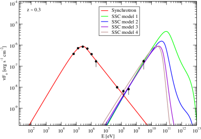
Figure 1: Synchrotron/SSC models for the GRB 940217 assuming $z\sim 0.3$.

2 One Zone Synchrotron/SSC Model and Fitting Technique

In the one zone synchrotron/SSC model for GRBs, a portion of a spherical shell, directed along our line of sight with Doppler factor $\delta_{\rm D}$, is assumed to be filled with nonthermal, isotropically-distributed electrons and ions, and to entrain a homogeneous, randomly-oriented magnetic field, $B$. When simulating synchrotron/SSC emission from GRBs, the usual method is to inject an electron distribution and allow it to evolve, and then simultaneously fit the entire SED by synchrotron and SSC components (Chiang and Dermer, 1999). This leads to a large number of parameters for the modeler to fit. We have developed a new approach, originally developed for TeV X-ray selected BL Lacertae objects (Finke et al., 2008). In this technique, the low-energy component is assumed to be synchrotron emission; by fitting this with an empirical function, one can directly obtain the electron distribution using the $\delta$-approximation for $\nu F_{\nu}$ synchrotron flux,

$$f_{\epsilon}^{syn}\cong{\delta_{\rm D}^{4}\over 6\pi d_{L}^{2}}\;c\sigma_{\rm T}U_{B}^{\prime}\gamma^{\prime 3}_{s}N_{e}^{\prime}(\gamma^{\prime}_{s})\ ,$$ (1)

(e.g., Dermer and Schlickeiser, 2002) where $d_{L}$ is the luminosity distance, $c$ is the speed of light, $U_{B}^{\prime}=B^{2}/(8\pi)$ is the magnetic field energy density, $\epsilon$ is the observed dimensionless photon energy, $\gamma^{\prime}_{s}=\sqrt{4\times 10^{13}\epsilon(1+z)/(\delta_{\rm D}B)}$ is the electron Lorentz factor, and $N_{e}^{\prime}(\gamma^{\prime}_{s})$ is the electron distribution. In the case of GRBs, the synchrotron spectrum is fit with the empirical representation of Band et al. (1993) which, in $\nu F_{\nu}$ flux, is

$$f_{\epsilon}^{syn}=\left\{\begin{array}[]{ll}f_{peak}\ \left[\frac{\epsilon}{\epsilon_{peak}}\right]^{a}\ \exp\left[-a\left(\frac{\epsilon}{\epsilon_{peak}}-1\right)\right]&\left(\epsilon\leq\frac{\epsilon_{peak}(a-b)}{a}\right)\\ f_{peak}\ \left[\frac{(a-b)\epsilon_{peak}}{a}\right]^{a-b}\ \frac{\epsilon^{b}}{\epsilon^{a}}\ e^{b}&\left(\epsilon>\frac{\epsilon_{peak}(a-b)}{a}\right)\end{array}\right.$$ (2)

where $f_{peak}=f_{\epsilon}^{syn}(\epsilon_{peak})$ and $a$ and $b$ are power-law indices. Once $N^{\prime}_{e}(\gamma^{\prime})$ is determined, the SSC flux can be calculated. We use the full Compton cross-section in the Thomson through Klein-Nishina regimes based on the formulae of Jones (1968). Assuming the redshift, $z$, of the burst is known, one can model the SSC emission as a function of a small set of parameters: $\delta_{\rm D}$, $B$, and $\Delta R^{\prime}$, the (comoving) size scale of the emitting region. The value of $\Delta R^{\prime}$ can be estimated from the observed variability time, $t_{var}$, based on light travel time arguments by $\Delta R^{\prime}=\delta_{\rm D}ct_{var}/(1+z)$, which effectively reduces the number of parameters in the fit to two. See Finke et al. (2008) for more details on this technique.

The “jet” power, the power available in the expanding shell that can create observed radiation, is a combination of the power in the nonthermal particles and in the magnetic field of the emitting region (Celotti and Fabian, 1993). It gives the upper limit on the observed isotropic luminosity, and is calculated by $L_{j}=2\pi\Delta R^{\prime}\beta\Gamma^{2}c\left(U_{B}^{\prime}+U_{p}^{\prime}\right)$, where $U_{p}^{\prime}$ is the particle energy density. The jet power can also allow one to constrain the magnetic field, by finding the magnetic field strength which minimizes this power (Dermer and Atoyan, 2004).

3 Example: Fits to GRB 940217

As an example of this technique, we fit the GRB 940217 with this synchrotron/SSC model. The Compton Gamma-Ray Observatory CGRO observed this GRB, one of the longest and most energetic GRBs to be detected at GeV energies.(Hurley et al., 1994). We include absorption by internal jet radiation (Gould and Schréder, 1967) and by the extragalactic background light (Stecker et al., 2006). The Band et al. (1993) fit to the synchrotron spectrum gives the parameters $a=1.2$, $b=-0.9$, $\epsilon_{peak}=0.53$, and $f_{peak}=8.8\times 10^{-7}$ erg s^-1 cm^-2. The redshift to the GRB 940217 is unknown; however, it can be estimated to be $z\sim 0.3$ based on the correlation of Atteia (2003). This redshift value is used in models 1 – 4 (Fig. 1), while the value $z\sim 1.0$ is used in models 5 – 8 (Fig. 2). The parameters for these models can be seen in Table 1. In all models, the variability timescale was taken to be 1 sec, consistent with CGRO observations (Hurley et al., 1994). These fits were done in a “$\chi$-by-eye” fashion, although for better data, $\chi^{2}$ minimization can be done (Finke et al., 2008).

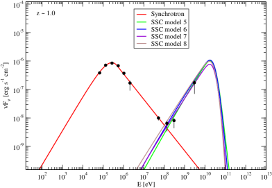
Figure 2: Synchrotron/SSC models for the GRB 940217 assuming $z\sim 1.0$.

At $z\sim 1.0$, the models are difficult to distinguish from each other, but at the lower redshift ($z\sim 0.3$), it is possible. although all of them give reasonable fits to the CGRO data. However, if the GRB had been observed by GLAST or a very high energy (VHE) $\gamma$-ray telescope, it would be possible to distinguish the models. Multiwavelength observations of future GRBs by Swift, GLAST, and VHE $\gamma$-ray telescopes such as MAGIC, VERITAS, and HESS will be key in discriminating between models. TeV $\gamma$-rays have not been conclusively detected from a GRB so far, and they would only be expected from nearby GRBs, as farther ones would have TeV radiation absorbed by the EBL.

At $z\sim 1.0$, the absorption is dominated by the EBL, and internal photoabsorption effects cannot be seen. However, the $z\sim 0.3$ models, while still dominated by EBL absorption, show curvature at TeV energies as a result of internal absorption. Such curvature in low-redshift GRBs is one of the key predictions of this model.

The GRB 940217 has an isotropic luminsosity of $L_{iso}\approx 3.1\times 10^{50}$ erg s^-1 if it is located at $z\sim 0.3$, and $L_{iso}\approx 5.0\times 10^{51}$ erg s^-1 if it is at $z\sim 1.0$. Models which have powers in excess of these can be excluded.

We have summarized a new technique for modeling synchrotron/SSC broadband spectral energy distributions of GRBs and applied it to the GRB 940217. Although the data for this burst is sparse and the redshift is unknown, this nonetheless illustrates the method. When applied to future multiwavelength observations, this technique will be a good tool for testing the validity of the synchrotron/SSC model.

Model	B [G]	$\delta_{D}$	$L_{j}$ [erg s-1]
1	0.07	460	$1.4\times 10^{55}$
2	1.0	370	$2.8\times 10^{53}$
3	13	330	$6.8\times 10^{51}$
4	141	310	$3.3\times 10^{50}$
5	0.01	930	$3.0\times 10^{56}$
6	0.87	740	$5.6\times 10^{54}$
7	10	680	$1.4\times 10^{53}$
8	114	640	$6.4\times 10^{51}$

Table 1: Model fit parameters

References

- Mészáros (2006) P. Mészáros, Reports of Progress in Physics 69, 2259–2322 (2006).
- Chiang and Dermer (1999) J. Chiang, and C. D. Dermer, ApJ 512, 699–710 (1999).
- Finke et al. (2008) J. D. Finke, C. D. Dermer, and M. Böttcher, ApJ, in preperation (2008).
- Dermer and Schlickeiser (2002) C. D. Dermer, and R. Schlickeiser, ApJ 575, 667–686 (2002).
- Band et al. (1993) D. Band, et al., ApJ 413, 281–292 (1993).
- Jones (1968) F. C. Jones, Physical Review 167, 1159–1169 (1968).
- Celotti and Fabian (1993) A. Celotti, and A. C. Fabian, MNRAS 264, 228–236 (1993).
- Dermer and Atoyan (2004) C. D. Dermer, and A. Atoyan, ApJ 611, L9–L12 (2004).
- Hurley et al. (1994) K. Hurley, et al., Nature 372, 652–654 (1994).
- Gould and Schréder (1967) R. J. Gould, and G. P. Schréder, Physical Review 155, 1404–1407 (1967).
- Stecker et al. (2006) F. W. Stecker, M. A. Malkan, and S. T. Scully, ApJ 648, 774–783 (2006).
- Atteia (2003) J.-L. Atteia, A&A 407, L1–L4 (2003).