Verfasser: Dipl.-Ing. Eberhard Mayerhofer
Matrikel-Nummer: 9540617
Dissertationsgebiet: Mathematik
Betreuer: Prof. Dr. Michael Kunzinger
Wien, am 1. August 2006

Abstract.
The first part of my thesis lays the foundations to generalized Lorentz geometry. The basic algebraic structure of finite-dimensional modules over the ring of generalized numbers is investigated. This includes a new characterization of invertibility in the ring of generalized numbers as well as a characterization of free elements inside the $n$-dimensional module $\widetilde{\mathbb{R}}^{n}$. The index of symmetric bilinear forms is introduced; this new concept enables a (generalized) pointwise characterization of generalized pseudo Riemannian metrics on smooth manifolds as introduced by M. Kunzinger and R. Steinbauer. It is shown that free submodules have direct summands, however $\widetilde{\mathbb{R}}^{n}$ turns out not to be semisimple. Applications of these new concepts are a generalized notion of causality, the generalized inverse Cauchy Schwarz inequality for time-like or null vectors, constructions of pseudo Riemannian metrics as well as generalized energy tensors. The motivation for this part of my thesis evolved from the main topic, the wave equation on singular space-times.

The second and main part of my thesis is devoted to establishing a local existence and uniqueness theorem for the wave equation on singular space-times. The singular Lorentz metric subject to our discussion is modeled within the special algebra on manifolds in the sense of J. F. Colombeau. Inspired by an approach to generalized hyperbolicity of conical-space times due to J. Vickers and J. Wilson, we succeed in establishing certain energy estimates, which by a further elaborated equivalence of energy integrals and Sobolev norms allow us to prove existence and uniqueness of local generalized solutions of the wave equation with respect to a wide class of generalized metrics.

The third part of my thesis treats three different point value resp. uniqueness questions in algebras of generalized functions. The first one, posed by Michael Kunzinger, reads as follows: Is the theorem by Albeverio et al., that elements of the so-called p-adic Colombeau Egorov algebra are determined uniquely on standard points, a p-adic scenario? We answer this problem by means of a counterexample which shows that the statement in fact does not hold. We further show that elements of an Egorov algebra of generalized functions on a locally compact ultrametric space allow a point-value characterization if and only if the metric induces the discrete topology. Secondly, we prove that the ring of generalized (real or complex) numbers endowed with the sharp norm does not admit nested sequences of closed balls to have an empty intersection. As an application we outline a possible version of the Hahn-Banach Theorem as well as the ultrametric Banach fixed point theorem. Finally, we establish that scaling invariant generalized functions on the real line are constant and we prove several new characterizations of locally constant generalized functions.

Preface

The present thesis represents my research work 2004-2006 in the field of generalized functions carried out under the supervision of Professor Michael Kunzinger at the Faculty of Mathematics, University of Vienna. All sections in this book have been the basis for scientific papers. For references concerning publication of this material I refer to the arxiv, where all of my submitted papers can be found, along with updated information concerning their publication status.

Vienna, February 2008 Eberhard Mayerhofer

Contents

1. 1 Introduction
   1. 1.1 Generalized functions and applications to relativity
      1. 1.1.1 The special algebra on manifolds
      2. 1.1.2 Generalized pseudo-Riemannian geometry
      3. 1.1.3 Generalized function concepts in general relativity
   2. 1.2 Uniqueness issues
2. 2 Algebraic foundations of Colombeau Lorentz geometry
   1. 2.1 Preliminaries
   2. 2.2 Causality and the inverse Cauchy-Schwarz inequality
   3. 2.3 Further algebraic properties of $\widetilde{\mathbb{R}}^{n}$
      1. 2.3.1 Direct summands of free submodules
      2. 2.3.2 $\widetilde{\mathbb{R}}^{n}$ is not semisimple
   4. 2.4 Energy tensors and a dominant energy condition
   5. 2.5 Point values and generalized causality
   6. 2.6 Appendix. Invertibility revisited
3. 3 The wave equation on singular space-times
   1. 3.1 Preliminaries
      1. 3.1.1 Constructions of Riemannian metrics from Lorentzian metrics
      2. 3.1.2 Energy tensors and dominant energy condition
      3. 3.1.3 The d’Alembertian in local coordinates
      4. 3.1.4 General Lorentzian metrics in suitable coordinates
      5. 3.1.5 The wave equation on a smooth space-time
      6. 3.1.6 Leray forms
      7. 3.1.7 Foliations and integration
   2. 3.2 Description of the method
   3. 3.3 The assumptions
      1. 3.3.1 Introduction. Generalized static space-times.
      2. 3.3.2 The setting. Assumptions on the metric
      3. 3.3.3 The setting. Formulation of the initial value problem
      4. 3.3.4 Locally foliated semi-neighborhoods.
      5. 3.3.5 Energy integrals and Sobolev norms
   4. 3.4 Equivalence: Energies and Sobolev norms
   5. 3.5 Bounds on initial energies
   6. 3.6 Energy inequalities
   7. 3.7 Bounds on energies
   8. 3.8 Sobolev estimates
   9. 3.9 Existence and uniqueness
   10. 3.10 Dependence on the metric representative
   11. 3.11 Possible generalizations
4. 4 Point values & uniqueness questions
   1. 4.1 Point values in Egorov algebras
      1. 4.1.1 A counterexample
      2. 4.1.2 Ultrametric Egorov algebras
      3. 4.1.3 Generalized point values
      4. 4.1.4 The $\delta$-distribution
   2. 4.2 Spherical completeness
      1. 4.2.1 Preliminaries
      2. 4.2.2 Euclidean models of sharp neighborhoods
      3. 4.2.3 The main theorem
      4. 4.2.4 A Hahn-Banach Theorem
   3. 4.3 Scaling invariance
      1. 4.3.1 Preliminaries
      2. 4.3.2 Functions supported at the origin
      3. 4.3.3 The main theorem
      4. 4.3.4 Scaling invariance in space.

Chapter 1 Introduction

Differential algebras of generalized functions in the sense of J. F. Colombeau provide a rigorous setting for treating numerous problems for which a general concept of multiplication of distributions is needed. Popular examples of such include partial differential equations with singular (in the sense of non-smooth, say distributional) data or coefficients: A sensible theory must admit singular solutions of the latter, therefore it is necessary to introduce a product of singular objects (in our example a singular coefficient times a singular solution); however, it is advisable to do this in a consistent way, meaning that on reasonable function subspaces of the distributions, the usual point-wise product coincides with such a product of singular objects, and is associative and commutative.

Many counterexamples support that on $\mathcal{D}^{\prime}$ such a product with values in $\mathcal{D}^{\prime}$ cannot exist (cf. [18], chapter 1). Let us consider the following: assume we were given an associative product $\circ$ on $\mathcal{D}^{\prime}$ and let $\mathop{\mathrm{vp}}(1/x)$ denote the principal value of $1/x$, then we would have

$$\delta=\delta\circ(x\circ\mathop{\mathrm{vp}}(1/x))=(\delta\circ x)\circ\mathop{\mathrm{vp}}(1/x)=0,$$

which is impossible, since $\delta\neq 0$. Apart from certain ”irregular (intrinsic or extrinsic) operations” (cf. [36]), there are basically two ways out of this dilemma:

1. We could restrict ourselves to strict subspaces of $\mathcal{D}^{\prime}$ which have a natural algebraic structure, for instance Sobolev spaces $\mathcal{H}^{s}(\mathbb{R}^{n})$ for $s>n/2$, $L_{loc}^{\infty},\,C^{k}$ etc., and

2. we could try to embed $\mathcal{D}^{\prime}$ into a larger space $\mathcal{G}$ which can be endowed with the structure of a differential algebra.

Since we want to multiply distributions unrestrictedly, we shall settle for (ii).

First we formulate the desired properties of a differential algebra $(\mathcal{G},\circ,+)$ containing the distributions. Let $\Omega\subset\mathbb{R}^{s}$ open. We wish to construct an associative, commutative algebra $({\mathcal{G}},+,\circ)$ such that:

1. There exists a linear embedding $\iota:{\mathcal{D}}^{\prime}\hookrightarrow{\mathcal{G}}$ such that $\iota(1)$ is the unit in ${\mathcal{G}}$.

2. There exist derivation operators $D_{i}:{\mathcal{G}}\to{\mathcal{G}}$ ($1\leq i\leq s$), which are linear and satisfy the Leibniz-rule.

3. $D_{i}\mid_{{\mathcal{D}}^{\prime}}=\frac{\partial}{\partial x_{i}}$ ($1\leq i\leq s$), that is the derivation operators restricted to $\mathcal{D}^{\prime}$ are the usual partial derivations.

4. $\circ\mid_{{\mathcal{C}}^{\infty}(\Omega)\times{\mathcal{C}}^{\infty}(\Omega)}$ is the point-wise product of functions.

Item (iv) corresponds to the above requirement that the new product should coincide with the usual point-wise product on a ”reasonable” subspace of $\mathcal{D}^{\prime}$. Schwartz’s famous impossibility result ([44]) states that such an algebra, does not exist, if the requirement (iv) is replaced by the respective requirement for continuous functions. Nevertheless J. F. Colombeau successfully constructed differential algebras $(\mathcal{G},+,\circ)$ satisfying (i)–(iv) ([9, 10]). Meanwhile there are a number of such algebras of generalized functions. For a general construction scheme, cf. [18]. In the following subsection we explain how the so-called special version on open sets of $\mathbb{R}^{n}$ is constructed. We then may introduce the special algebra on manifolds and we shall discuss its relevance for applications in general relativity. The chapter will end with an introduction to point-value concepts in algebras of generalized functions.

Colombeau’s special algebra

Let $\Omega$ be an open subset of $\mathbb{R}^{d}$. The so-called special Algebra due to J. F. Colombeau is given by the quotient

$$\mathcal{G}(\Omega):=\mathcal{E}_{M}(\Omega)/\mathcal{N}(\Omega),$$

where the (ring of) moderate functions $\mathcal{E}_{M}(\Omega)$ resp. the ring of negligible elements (being an ideal in $\mathcal{E}_{M}(\Omega)$) are given by

$$\!\!\mathcal{E}_{M}(\Omega)\!\! := \!\!\{(u_{\varepsilon})_{\varepsilon}\in C^{\infty}(\Omega)^{(0,1]}|\forall K\subset\subset\Omega\,\forall\alpha\,\exists\,N\ \sup_{x\in K}|\partial^{\alpha}u_{\varepsilon}(x)|=O(\varepsilon^{-N})\}$$

$$\!\!\mathcal{N}(\Omega)\!\! := \!\!\{(u_{\varepsilon})_{\varepsilon}\in C^{\infty}(\Omega)^{(0,1]}|\forall K\subset\subset\Omega\,\forall\alpha\,\forall\,m\ \sup_{x\in K}|\partial^{\alpha}u_{\varepsilon}(x)|=O(\varepsilon^{m})\}.$$

The algebraic operations ($+,\circ$) as well as (partial) differentiation, composition of functions etc. are meant to be performed component-wise on the level of representatives; the transfer to the quotient $\mathcal{G}(\Omega)$ is then well defined (cf. the comprehensive presentation in the first chapter of [18]). Once a Schwartz mollifier $\rho$ on $\mathbb{R}^{d}$ with all moments vanishing has been chosen, the space of compactly supported distributions may be embedded into $\mathcal{G}(\Omega)$ via convolution; an embedding of all of $\mathcal{D}^{\prime}(\Omega)$ into our algebra is achieved via a partition of unity using sheaf theoretic arguments, therefore being not canonical.

1.1. Algebras of generalized functions on manifolds and applications in general relativity

The aim of this section is to review the basics of the special algebra on manifolds $X$ as well as the definitions of generalized sections of vector bundles with base space $X$ and we recall the definition of generalized pseudo-Riemannian metrics. At the end of the section we motivate the use of differential algebras for applications in relativity, in particular for the wave equation on singular space-times which is treated in the present book.

1.1.1. The special algebra on manifolds

Similarly as in section 1 one may define algebras of generalized functions on manifolds. We start first by introducing the special algebra on manifolds in a coordinate independent way as in [28]. However, for two reasons we shall later translate the definitions into respective definitions in terms of coordinate expressions: For for the sake of clarity and simplicity, but also for the following purpose: In chapter 3 we shall perform estimates in a coordinate patch in order to derive a (local) existence result for the Cauchy problem of the wave equation in a generalized setting.

The material presented here stems from the original sources [28, 30]. For a comprehensive presentation we refer to the–meanwhile standard reference on generalized function algebras – [18]. Moreover, for further works in geometry based on Colombeau’s ideas we refer to ([20, 25, 27, 29, 30, 32, 33]).

For what follows in this section, $X$ shall denote a paracompact, smooth Hausdorff manifold of dimension $n$ and by $\mathcal{P}(X)$ we denote the space of linear differential operators on $X$. The special algebra of generalized functions on $X$ is constructed as the quotient $\mathcal{G}(X):=\mathcal{E}_{M}(X)/\mathcal{N}(X)$, where the ring of moderate (resp. negligible) functions is given by

$$\mathcal{E}_{M}(X):=\{(u_{\varepsilon})_{\varepsilon}\in(C^{\infty}(X))^{I}\mid\forall\;K\subset\subset X\;\forall\;P\in\mathcal{P}(X)\;\exists\;N\in\mathbb{N}:$$

(1.1) $$\sup_{x\in K}|Pu_{\varepsilon}|=O(\varepsilon^{-N})\,(\varepsilon\rightarrow 0)$$

resp.

$$\mathcal{N}(X):=\{(u_{\varepsilon})_{\varepsilon}\in(C^{\infty}(X))^{I}\mid\forall\;K\subset\subset X\;\forall\;P\in\mathcal{P}(X)\;\forall\;m\in\mathbb{N}:$$

(1.2) $$\sup_{x\in K}|Pu_{\varepsilon}|=O(\varepsilon^{m})\,(\varepsilon\rightarrow 0).$$

The $C^{\infty}$ sections of a vector bundle $(E,X,\pi)$ with base space $X$ we denote by $(E,X,\pi)$. Moreover, let $\mathcal{P}(X,E)$ be the space of linear partial differential operators acting on $\Gamma(X,E)$. The $\mathcal{G}(X)$ module of generalized sections $\Gamma_{\mathcal{G}}(X,E)$ of a vector bundle $(E,X,\pi)$ on $X$ is defined similarly as (the algebra of generalized functions on $X$) above, in that we use asymptotic estimates with respect to the norm induced by some arbitrary Riemannian metric on the respective fibers, that is, we define the quotient

$$\Gamma_{\mathcal{G}}(X,E):=\Gamma_{\mathcal{E}_{M}}(X,E)/\Gamma_{\mathcal{N}}(X,E),$$

where the ring (resp. ideal) of moderate (resp. negligible) nets of sections is given by

$$\Gamma_{\mathcal{E}_{M}}(X,E):=\{(u_{\varepsilon})_{\varepsilon}\in(\Gamma(X,E))^{I}\mid\forall\;K\subset\subset X\;\forall\;P\in\mathcal{P}(X,E)\;\exists\;N\in\mathbb{N}:$$

(1.3) $$\sup_{x\in K}\|Pu_{\varepsilon}\|=O(\varepsilon^{N})\,(\varepsilon\rightarrow 0)$$

resp.

$$\Gamma_{\mathcal{N}}(X,E):=\{(u_{\varepsilon})_{\varepsilon}\in(\Gamma(X,E))^{I}\mid\forall\;K\subset\subset X\;\forall\;P\in\mathcal{P}(X,E)\;\forall\;m\in\mathbb{N}:$$

(1.4) $$\sup_{x\in K}\|Pu_{\varepsilon}\|=O(\varepsilon^{m})\,(\varepsilon\rightarrow 0).$$

In this book we shall deal with generalized sections of the tensor bundle $\mathcal{T}^{r}_{s}(X)$ over $X$, this we denote by

$$\mathcal{G}^{r}_{s}(X):=\Gamma_{\mathcal{G}}(X,\mathcal{T}^{r}_{s}(X)).$$

Elements of the latter we call generalized tensors of type $(r,s)$. We end this section by translating the global description of generalized vector bundles in terms of coordinate expressions. Following the notation of [30], we denote by $(V,\Psi)$ a vector bundle chart over a chart $(V,\psi)$ of the base $X$. With $\mathbb{R}^{n^{\prime}}$, the typical fibre, we can write:

$$\Psi:\pi^{-1}(V)\rightarrow\psi(V)\times\mathbb{R}^{n^{\prime}},$$

$$z\mapsto(\psi(p),\psi^{1}(z),\dots,\psi^{n^{\prime}}(z)).$$

Let now $s\in\Gamma_{\mathcal{G}}(X,E)$. Then the local expressions of $s$, $s^{i}=\Psi^{i}\circ s\circ\psi^{-1}$ lie in $\mathcal{G}(\psi(V))$.

An equivalent ”local definition” of generalized vector bundles can be achieved by defining moderate nets $(s_{\varepsilon})_{\varepsilon}$ of smooth sections $s_{\varepsilon}$ to be such for which the local expressions $s_{\varepsilon}^{i}=\Psi^{i}\circ s_{\varepsilon}\circ\psi^{-1}$ are moderate, that is $(s_{\varepsilon}^{i})_{\varepsilon}\in\mathcal{E}_{M}(\psi(V))$. The notion negligible is defined completely similar. The proof of this fact can be achieved by using Peetre’s theorem (cf. [18], p. 289).

1.1.2. Generalized pseudo-Riemannian geometry

We begin with recalling the following characterization of non-degenerateness of symmetric (generalized) tensor fields of type (0,2) on $X$ ([31], Theorem 3. 1). For a characterization of invertibility of generalized functions we refer to Proposition 2. 1 of [31] and for a further characterization we refer to the appendix of chapter 2 (namely Theorem 2.46).

Theorem 1.1.

Let $g\in\mathcal{G}^{0}_{2}(X)$. The following are equivalent:

1. For each chart $(V_{\alpha},\psi_{\alpha})$ and each $\widetilde{x}\in(\psi_{\alpha}(V_{\alpha}))^{\sim}_{c}$ the map $g_{\alpha}(\widetilde{x}):\widetilde{\mathbb{R}}^{n}\times\widetilde{\mathbb{R}}^{n}\rightarrow\widetilde{\mathbb{R}}$ is symmetric and non-degenerate.

2. $g:\mathcal{G}^{0}_{1}(X)\times\mathcal{G}^{0}_{1}(X)\rightarrow\mathcal{G}(X)$ is symmetric and $\det(g)$ is invertible in $\mathcal{G}(X)$.

3. $\det g$ is invertible in $\mathcal{G}(X)$ and for each relatively compact open set $V\subset X$ there exists a representative $(g_{\varepsilon})_{\varepsilon}$ of $g$ and $\varepsilon_{0}>0$ such that $g_{\varepsilon}\mid_{V}$ is a smooth pseudo-Riemannian metric for all $\varepsilon<\varepsilon_{0}$.

Furthermore, the index of $g\in\mathcal{G}^{0}_{2}(X)$ is introduced in the following well defined way (cf. Definition 3. 2 and Proposition 3. 3 in [31]):

Definition 1.2.

Let $g\in\mathcal{G}^{0}_{2}(X)$ satisfy one (hence all) of the equivalent conditions in Theorem 1.1. If there exists some $j\in\mathbb{N}$ with the property that for each relatively compact open set $V\subset X$ there exists a representative $(g_{\varepsilon})_{\varepsilon}$ of $g$ as in Theorem 1.1 (iii) such for each $\varepsilon<\varepsilon_{0}$ the index of $g_{\varepsilon}$ is equals $j$ we say $g$ has index $j$. Such symmetric 2-forms we call generalized pseudo-Riemannian metrics on $X$.

We shall work in generalized space-times. These are pairs $(\mathcal{M},g)$, where $\mathcal{M}$ is an orientable paracompact four dimensional smooth manifold and $g$ is a symmetric generalized (0,2) tensor with invertible $\det g$ (cf. Theorem 1.1) and index $\nu=1$. In chapter 2 we develop algebraic foundations of generalized Lorentz geometry; here the emphasis lies on considering Lorentz metrics from a generalized point of view and to develop causality notions in the generalized context. In the subsequent chapter 3 we use the so found new concepts to define and work with space-time symmetries, namely (smooth) time-like Killing vector fields $\xi$ with respect to a generalized metric $g$ (cf. Definition 3.15 and the subsequent elaboration).

We end this section with reviewing the notion of generalized connections and curvature ([30], section 5).

A generalized connection $\hat{D}$ is a mapping $\mathcal{G}^{1}_{0}(\mathcal{M})\times\mathcal{G}^{1}_{0}(\mathcal{M})\rightarrow\mathcal{G}^{1}_{0}(\mathcal{M})$ satisfying (for the notion of generalized Lie derivative, cf. [30])

1. $\hat{D}_{\xi}\eta$ is $\widetilde{\mathbb{R}}$–linear in $\eta$,

2. $\hat{D}_{\xi}\eta$ is $\mathcal{G}(\mathcal{M})$–linear in $\xi$ and

3. $\hat{D}_{\xi}(u\eta)=u\hat{D}_{\xi}\eta+\xi(u)\eta$ for all $u$ in $\mathcal{G}(\mathcal{M})$.
   In analogy with the standard pseudo-Riemannian geometry, the connection is unique provided the following additional conditions are satisfied (cf. [30], Theorem 5.2). For arbitrary $\xi,\eta,\zeta\in\mathcal{G}^{1}_{0}(\mathcal{M})$ we have:

4. $[\xi,\eta]=\hat{D}_{\xi}\eta-\hat{D}_{\eta}\xi$ and

5. $\xi g(\eta,\zeta)=g(D_{\xi}\eta,\zeta)+g(\eta,D_{\xi}\zeta)$.

In terms of coordinate expressions, the connection can be written down by means of ”generalized” Christoffel symbols: Assume we are given a chart $(V_{\alpha},\psi_{\alpha})$ on $\mathcal{M}$ with coordinates $x^{i}$ $(i=1,\dots,4)$. The Christoffel symbols are generalized functions $\Gamma_{ij}^{k}\in\mathcal{G}(V_{\alpha})$ defined by

$$\hat{D}_{\partial_{i}}\partial_{j}=\Gamma_{ij}^{k}\partial_{k},\qquad 1\leq i,j\leq n.$$

1.1.3. Generalized function concepts in general relativity

Even
though sufficient motivation to study the Cauchy problem of the wave equation on a space-time whose metric is of lower differentiability may emerge from a purely mathematical interest, our original motivation actually stems from physics. The aim of this section is to answer the following two questions: ”Why do we intend to solve the wave equation on a singular space-time” and, ”Why do we employ generalized function algebras for this matter?”.

The field of general relativity is a non-linear theory, in the sense that the curvature depends non-linearly on the metric and its derivatives. This results in several problems when one comes to consider the concept of singularities in space-times:

1. Firstly, from a mathematical point of view, an immediate problem when a singular space–time is modeled by means of a distributional metric, is: In the coordinate formula for the Christoffel symbols (hence in the formula for the curvature), products of the metric coefficients and their derivatives occur, and a (distributional) meaning has to be given to the latter. As outlined above, this is not always possible in the framework of distributions, because they form a linear theory ( cf. the discussion at the beginning of the chapter).

2. The second natural obstacle is the difficulty of distinguishing ”strong” singularities from ”weak” singularities. Singularities were originally defined as endpoints of incomplete geodesics, which could not be extended such that the differentiability of the resulting space-time remained $C^{2-}$ (cf. Hawking and Ellis, [21]). The class of singularities defined in this manner unfortunately includes both genuine gravitational singularities such as Schwarzschild and ”weaker” singularities as in conical space-times, impulsive gravitational waves and shell crossing singularities. A recent idea put forward by C. J. S. Clarke in ([7]) supports a new concept of ”weak” singularities: A singularity in a space-time should only be considered essential if it disrupts the evolution of linear test fields. According to this idea, Clarke calls a space-times generalized hyperbolic, if the Cauchy problem for the scalar wave equation is well posed, and then shows that space-times with locally integrable curvature are in this class.

Vickers and Wilson are the first authors who apply Clarke’s concepts by showing that conical space-times are generalized hyperbolic (cf. [49]; in the context of generalized function algebras this is called $\mathcal{G}$–generalized hyperbolic). To further overcome obstacle (i) in a mathematically rigorous way, they reformulate the Cauchy problem in the full Colombeau algebra. Finally, they show that the resulting generalized solution is associated with a distributional solution (this can be done by considering weak limits with respect to the smoothing parameter $\varepsilon$, cf. the definitions given in section 4.3.1).

We shall follow Vickers’ and Wilson’s approach and try to generalize their result to a wide range of generalized space-times in chapter 3. However, it should be noted that contrary to [49], we work in the special algebra exclusively. Moreover, the technique we are using (based on certain energy integrals and Sobolev norms) lies somewhere between Hawking and Ellis’ method ([21]) and Vickers’ and Wilson’s.

For more information on the use of generalized function algebras in relativity we refer to the recent review [46] on this topic by R. Steinbauer and J. Vickers as well as J. Vickers’s article ([17] pp. 275–290) and the introduction to [49]. For relativistic applications in the framework of Colombeau’s theory, see [8, 18, 19].

1.2. Uniqueness issues in algebras of generalized functions

The last chapter of the present work consists of three different problems which we have summarized under the title ”point values and uniqueness questions in algebras of generalized functions”. Even though the problems are quite different, they all have to do with the basic question: ”given two generalized functions $f,g$, how can we decide if $f=g$?” It is clear that we can reduce this to the problem of determining whether a generalized function $h$ vanishes identically. Before we come to a possible answer offered by M. Kunzinger and M. Oberguggenberger in [38] in form of a ”uniqueness test” via evaluation of generalized functions on so-called compactly supported points, we motivate the problem from the distributional point of view.

By definition, a distribution $w\in\mathcal{D}^{\prime}$ is zero if the test with arbitrary test functions $\phi$ yields $\langle w,\phi\rangle=0$. The question, reformulated in the context of the special algebra, reads, ”is the embedded object $\iota(w)\in\mathcal{G}$ identically zero?”.

However, since the key idea of embedding distributions into $\mathcal{G}$ is regularization of the latter, we shall leave aside the embedding and answer this question for regularized nets of distributions in terms of the following characterization:

Theorem 1.3.

Let $u\in\mathcal{D}^{\prime}(\mathbb{R}^{n})$ and let $\rho\in\mathcal{D}(\mathbb{R}^{n})$ be a standard mollifier, that is, with $\int\rho(x)\;dx^{n}=1$ and let $\rho_{\varepsilon}(x):=\frac{1}{\varepsilon^{n}}\rho(\frac{x}{\varepsilon})$. The following are equivalent:

1. $u=0$ in $\mathcal{D}^{\prime}(\mathbb{R}^{n})$.

2. For each compactly supported net $(x_{\varepsilon})_{\varepsilon}\in(\mathbb{R}^{n})^{(0,1]}$ we have

   $$(u\ast\rho_{\varepsilon})(x_{\varepsilon})\rightarrow 0\qquad\mbox{if}\qquad\varepsilon\rightarrow 0.$$

Proof.

The implication (i)$\Rightarrow$(ii) is obvious, since for each $\varepsilon>0$ and each $x\in\mathbb{R}^{n}$, $\rho_{\varepsilon}\ast u(x)=\langle u(y),\rho_{\varepsilon}(\frac{x-y}{\varepsilon})\rangle=0$. To show the converse direction, assume $u\neq 0$ but that (ii) holds. Then there exists $\phi\in\mathcal{D}(\mathbb{R}^{n})$ such that $\langle u,\phi\rangle\neq 0$. It follows that there exists a positive constant $C_{1}$ and an index $\varepsilon_{0}\in(0,1]$ such that for each $\varepsilon<\varepsilon_{0}$ we have

(1.5) $$\left|\int(u\ast\rho_{\varepsilon})\,\phi\;dx^{n}\right|\geq C_{1}.$$

Therefore there exist a sequence $\varepsilon_{k}\rightarrow 0$ in $(0,1]$, a compactly supported sequence $x_{\varepsilon_{k}}\in\mathbb{R}^{n}$ and a positive number $C$ such that for each $k\geq 1$ we have

(1.6) $$|u\ast\rho_{\varepsilon_{k}}(x_{\varepsilon_{k}})|\geq C.$$

Indeed, if we assume the contrary, then for each set $K\subset\subset\mathbb{R}^{n}$ we would have $\sup_{x\in K}|u\ast\rho_{\varepsilon}|\rightarrow 0$ whenever $\varepsilon\rightarrow 0$. Fix $K$ such that $\mathop{\mathrm{supp}}\phi\subseteq K$. Then we have

$$\left|\int(u\ast\rho_{\varepsilon})\,\phi\;dx^{n}\right|\leq\mathop{\mathrm{vol}}(K)\|\phi\|_{\infty}\|u\ast\rho_{\varepsilon}\|_{K,\infty}\rightarrow 0$$

whenever $\varepsilon\rightarrow 0$, a contradiction to (1.5).

Finally define $(x_{\varepsilon})_{\varepsilon}$ as follows: $x_{\varepsilon}:=x_{\varepsilon_{k}}$ whenever $\varepsilon\in(\varepsilon_{k+1},\varepsilon_{k}]$ ($k\geq 1)$ and $x_{\varepsilon}:=x_{\varepsilon_{1}}$ when $\varepsilon\in(x_{1},1]$. By (1.6) we have a contradiction to our assumption. Therefore $u=0$ and we are done. ∎

It is further evident that, in the above characterization, (ii) cannot be replaced by the condition
For each $x\in\mathbb{R}^{n}$ we have

$$(u\ast\rho_{\varepsilon})(x)\rightarrow 0\quad\mbox{whenever}\quad\varepsilon\rightarrow 0.$$

To see this, take a standard mollifier $\rho$ with support $\mathop{\mathrm{supp}}\rho=[0,1]$. Then for each $x$ there exists an index $\varepsilon_{0}$ such that $\rho_{\varepsilon}(x)=0$ for each $\varepsilon<\varepsilon_{0}$. But for $\varepsilon\rightarrow 0$ we have

$$\rho_{\varepsilon}\rightarrow\delta\qquad\mbox{in}\qquad\mathcal{D}^{\prime}.$$

We go on now by showing how these ideas are elaborated in the context of the special algebra:

The generalized point values concept

Generalized functions can be evaluated at standard points. To be more precise, let us introduce the ring of generalized numbers $\widetilde{\mathbb{R}}$, defined by the quotient

$$\widetilde{\mathbb{R}}:=\mathcal{E}_{M}/\mathcal{N},$$

where the ring of moderate numbers

$$\mathcal{E}_{M}:=\{(x_{\varepsilon})_{\varepsilon}\in\mathbb{R}^{(0,1]}:\exists\,N:\;|x_{\varepsilon}|=O(\varepsilon^{-N})\}.$$

Similarly the ideal of negligible numbers $\mathcal{N}$ in $\mathcal{E}_{M}$ is given by

$$\mathcal{N}:=\{(x_{\varepsilon})_{\varepsilon}\in\mathbb{R}^{(0,1]}:\forall\,m:\;|x_{\varepsilon}|=O(\varepsilon^{m})\}.$$

Let $\widetilde{\mathbb{R}}_{c}$ denote the set of compactly supported elements of $\widetilde{\mathbb{R}}$, that is: $x_{c}$ lies in $\widetilde{\mathbb{R}}_{c}$ if and only if there exists a compact set $K\subseteq\mathbb{R}$ such that for one (hence any) representative $(x_{\varepsilon})_{\varepsilon}$ there exists an index $\varepsilon_{0}$ such that for all $\varepsilon<\varepsilon_{0}$ we have $x_{\varepsilon}\in K$. It can easily be shown that evaluation of generalized functions $f$ on compactly supported generalized points makes perfect sense in the following way: let $(f_{\varepsilon})_{\varepsilon}$ be a representative of $f\in\mathcal{G}(\mathbb{R})$, then

$$\widetilde{f}(x_{c}):=(f_{\varepsilon}(x_{\varepsilon}))_{\varepsilon}+\mathcal{N}\in\widetilde{\mathbb{R}}$$

yields a well defined generalized number. We denote by $\widetilde{f}:\widetilde{\mathbb{R}}_{c}\rightarrow\widetilde{\mathbb{R}}$ the above map induced by the generalized function $f$.

By a standard point $x$ we shall mean an element of $\widetilde{\mathbb{R}}$ which admits a constant representative, i. e. $x=(\alpha)_{\varepsilon}+\mathcal{N}$ for a certain real number $\alpha$. M. Kunzinger and M. Oberguggenberger show in ([38]) that it does not suffice to know the values of generalized functions at standard points in order to determine them uniquely. Furthermore, the following analog of Theorem 1.3 holds:

Theorem 1.4.

Let $f\in\mathcal{G}(\mathbb{R})$. The following are equivalent:

1. $f=0$ in $\mathcal{G}(\mathbb{R})$,

2. $\forall\;x_{c}\;\in\widetilde{\mathbb{R}}_{c}:\;\widetilde{f}(x_{c})=0$.

Note that a similar statement holds in Egorov algebras (cf. the final remark in [38]). In the first section of chapter 4 we show that also in $p$-adic Egorov algebras such a characterization holds and that evaluation at standard points does not suffice to determine elements of such algebras uniquely. In section 4.2 we elaborate a topological question in the ring of generalized numbers $\widetilde{\mathbb{R}}$ endowed with the so-called sharp topology. Finally, in the end of chapter 4, we apply some new differential calculus on $\widetilde{\mathbb{R}}$ due to Aragona ([4]) for showing that the only scaling invariant functions on the real line are the constants.

Chapter 2 Algebraic foundations of Colombeau Lorentz geometry

In the course of chapter 3 we shall establish a local existence and uniqueness theorem for the Cauchy problem of the wave equation in a generalized context. The considerations we had to undertake to achieve this result showed that a generalized concept of causality might be useful to describe scenarios in a non-smooth space-time without always having to deal merely with the standard concepts component-wise on the level of representatives. However, also from a purely theoretical point of view, the need of a such a concept becomes clear: the non-standard aspect in Colombeau theory, which gives rise to a description of objects not point-wise but on so-called generalized points (cf. [38] and chapter 4). This has been taken up in the recent and initial work by M. Kunzinger and R. Steinbauer on generalized pseudo-Riemannian geometry ([31]), on which we base our considerations (cf.  the assumptions on the metric in section 3.3.2), but it has not yet been investigated to a wide extent. For instance, invertibility of generalized functions has been characterized (cf. [31], Proposition 2. 1) and allowed a notable characterization of symmetric generalized non-degenerate $(0,2)$ forms (cf. Theorem 1.1). But so far there has not been given a characterization of generalized pseudo-Riemannian metrics $h$ in terms of bilinear forms $\widetilde{h}$ stemming from evaluation of $h$ at compactly supported points (on the respective manifold).

The main aim of this chapter, therefore, is to describe and discuss some elementary questions of generalized pseudo-Riemannian geometry under the aspect of generalized points. Our program is as follows: Introducing the index of a symmetric bilinear form on the $n$-dimensional module $\widetilde{\mathbb{R}}^{n}$ over the generalized numbers $\widetilde{\mathbb{R}}$ enables us to define the appropriate notion of a bilinear form of Lorentz signature. We can therefore propose a notion of causality in this context. The general statement of the inverse Cauchy-Schwartz inequality is then given. We further show that a dominant energy condition in the sense of Hawking and Ellis for generalized energy tensors (such as also indirectly assumed in [49]) is satisfied. We also answer the algebraic question: ”Does any submodule in $\widetilde{\mathbb{R}}^{n}$ have a direct summand?”: For free submodules, the answer is positive and is basically due to a new characterization of free elements in $\widetilde{\mathbb{R}}^{n}$. In general, however, direct summands do not exist: $\widetilde{\mathbb{R}}^{n}$ is not semisimple. In the end of the chapter we present a new characterization of invertibility in algebras of generalized functions. Finally, we want to point out that the positivity issues on the ring of generalized numbers treated here have links to papers by M. Oberguggenberger et al. ([22, 35]).

2.1. Preliminaries

Let $I:=(0,1]\subseteq\mathbb{R}$, and let $\mathbb{K}$ denote $\mathbb{R}$ resp. $\mathbb{C}$. The ring of generalized numbers over $\mathbb{K}$ is constructed in the following way: Given the ring of moderate nets of numbers $\mathcal{E}(\mathbb{K}):=\{(x_{\varepsilon})_{\varepsilon}\in\mathbb{K}^{I}\mid\exists\;m:|x_{\varepsilon}|=O(\varepsilon^{m})\,(\varepsilon\rightarrow 0)\}$ and, similarly, the ideal of negligible nets in $\mathcal{E}(\mathbb{K})$ which are of the form $\mathcal{N}(\mathbb{K}):=\{(x_{\varepsilon})_{\varepsilon}\in\mathbb{K}^{I}\mid\forall\;m:|x_{\varepsilon}|=O(\varepsilon^{m})\,(\varepsilon\rightarrow 0)\}$, we may define the generalized numbers as the factor ring $\widetilde{\mathbb{K}}:=\mathcal{E}_{M}(\mathbb{K})/\mathcal{N}(\mathbb{K})$. An element $\alpha\in\widetilde{\mathbb{K}}$ is called strictly positive if it lies in $\widetilde{\mathbb{R}}$ (this means that for any representative $(\alpha_{\varepsilon})_{\varepsilon}=(\mathop{\mathrm{Re}}(\alpha_{\varepsilon}))_{\varepsilon}+i(\mathop{\mathrm{Im}}(\alpha_{\varepsilon}))_{\varepsilon}$ we have $(\mathop{\mathrm{Im}}(\alpha_{\varepsilon}))_{\varepsilon}\in\mathcal{N}(\mathbb{R})$) and if $\alpha$ has a representative $(\alpha_{\varepsilon})_{\varepsilon}$ such that there exists $m\geq 0$ such that $\mathop{\mathrm{Re}}(\alpha_{\varepsilon})\geq\varepsilon^{m}$ for each $\varepsilon\in I=(0,1]$, we shall write $\alpha>0$. Clearly any strictly positive number is invertible. $\beta\in\widetilde{\mathbb{R}}$ is called strictly negative, if $-\beta>0$. Note that a generalized number $u$ is strictly positive precisely when it is invertible (due to [31] Proposition 2. 2 this means that $u$ is strictly non-zero) and positive (i. e., $u$ has a representative $(u_{\varepsilon})_{\varepsilon}$ which is greater or equals zero for each $\varepsilon\in I$). In the appendix to this chapter a new and somewhat surprising characterization of invertibility and strict positivity in the frame of the special algebra construction is presented.

Let $A\subset I$, then the characteristic function $\chi_{A}\in\widetilde{\mathbb{R}}$ is given by the class of $(\chi_{\varepsilon})_{\varepsilon}$, where

$$\chi_{\varepsilon}:=\begin{cases}1,\qquad\mbox{if}\qquad\varepsilon\in A\\ 0,\qquad\mbox{otherwise}\end{cases}.$$

Whenever $\widetilde{\mathbb{R}}^{n}$ is involved, we consider it as an $\widetilde{\mathbb{R}}$–module of dimension $n\geq 1$. Clearly the latter can be identified with $\mathcal{E}_{M}(\mathbb{R}^{n})/\mathcal{N}({\mathbb{R}^{n}})$, but we will not often use this fact subsequently. Finally, we denote by $\widetilde{\mathbb{R}}^{n^{2}}:=\mathcal{M}_{n}(\widetilde{\mathbb{R}})$ the ring of $n\times n$ matrices over $\widetilde{\mathbb{R}}$. A matrix $A$ is called orthogonal, if $UU^{t}=\mathbb{I}$ in $\widetilde{\mathbb{R}}^{n^{2}}$ and $\det U=1$ in $\widetilde{\mathbb{R}}$. Clearly, there are two different ways to introduce $\widetilde{\mathbb{R}}^{n^{2}}$:

Remark 2.1.

Denote by $\mathcal{E}_{M}(\mathcal{M}_{n}(\mathbb{R}))$ the ring of moderate nets of $n\times n$ matrices over $\mathbb{R}$, a subring of $\mathcal{M}_{n}(\mathbb{R})^{I}$. Similarly let $\mathcal{N}(\mathcal{M}_{n}(\mathbb{R}))$ denote the ideal of negligible nets of real $n\times n$ matrices. There is a ring isomorphism $\varphi:\widetilde{\mathbb{R}}^{n^{2}}\rightarrow\mathcal{E}_{M}(\mathcal{M}_{n}(\mathbb{R}))/\mathcal{N}(\mathcal{M}_{n}(\mathbb{R}))$.

For the convenience of the reader we repeat Lemma 2. 6 from [31]:

Lemma 2.2.

Let $A\in\widetilde{\mathbb{R}}^{n^{2}}$. The following are equivalent:

1. $A$ is non-degenerate, that is, $\xi\in\widetilde{\mathbb{R}}^{n},\;\xi^{t}A\eta=0$ for each $\eta\in\widetilde{\mathbb{R}}^{n}$ implies $\xi=0$.

2. $A:\widetilde{\mathbb{R}}^{n}\rightarrow\widetilde{\mathbb{R}}^{n}$ is injective.

3. $A:\widetilde{\mathbb{R}}^{n}\rightarrow\widetilde{\mathbb{R}}^{n}$ is bijective.

4. $\det A$ is invertible in $\widetilde{\mathbb{R}}$.

Note that the equivalence of (i)–(iii) and (iv) results from the fact that in $\widetilde{\mathbb{R}}$ any nonzero non-invertible element is a zero-divisor. Since we deal with symmetric matrices throughout, we start by giving a basic characterization of symmetry of generalized matrices:

Lemma 2.3.

Let $A\in\widetilde{\mathbb{R}}^{n^{2}}$. The following are equivalent:

1. $A$ is symmetric, that is $A=A^{t}$ in $\widetilde{\mathbb{R}}^{n^{2}}$.

2. There exists a symmetric representative $(A_{\varepsilon})_{\varepsilon}:=((a_{ij}^{\varepsilon})_{ij})_{\varepsilon}$ of $A$.

Proof.

Since (ii) $\Rightarrow$ (i) is clear, we only need to show (i) $\Rightarrow$ (ii). Let $((\bar{a}_{ij}^{\varepsilon})_{ij})_{\varepsilon}$ a representative of $A$. Symmetrizing yields the desired representative

$$(a_{ij}^{\varepsilon})_{\varepsilon}:=\frac{(\bar{a}_{ij}^{\varepsilon})_{\varepsilon}+(\bar{a}_{ji}^{\varepsilon})_{\varepsilon}}{2}$$

of $A$. This follows from the fact that for each pair $(i,j)\in\{1,\dots,n\}^{2}$ of indices one has $(\bar{a}_{ij}^{\varepsilon})_{\varepsilon}-(\bar{a}_{ji}^{\varepsilon})_{\varepsilon}\in\mathcal{N}(\mathbb{R})$ due to the symmetry of $A$. ∎

Denote by $\|\,\|_{F}$ the Frobenius norm on $\mathcal{M}_{n}(\mathbb{C})$. In order to prepare a notion of eigenvalues for symmetric matrices, we repeat a numeric result given in [47] (Theorem 5. 2):

Theorem 2.4.

Let $A\in\mathcal{M}_{n}(\mathbb{C})$ be a Hermitian matrix with eigenvalues $\lambda_{1}\geq\dots\geq\lambda_{n}$. Denote by $\widetilde{A}$ a non-Hermitian perturbation of $A$, i. e., $E=\widetilde{A}-A$ is not Hermitian. We further call the eigenvalues of $\widetilde{A}$ (which might be complex) $\mu_{k}+i\nu_{k}\;(1\leq k\leq n)$ where $\mu_{1}\geq\dots\geq\mu_{n}$. In this notation, we have

$$\sqrt{\sum_{k=1}^{n}|(\mu_{k}+i\nu_{k})-\lambda_{k}|^{2}}\leq\sqrt{2}\|E\|_{F}.$$

Definition 2.5.

Let $A\in\widetilde{\mathbb{R}}^{n^{2}}$ be a symmetric matrix and let $(A_{\varepsilon})_{\varepsilon}$ be an arbitrary representative of $A$. Let for any $\varepsilon\in I$, $\theta_{k,\varepsilon}:=\mu_{k,\varepsilon}+i\nu_{k,\varepsilon}\;(1\leq k\leq n)$ be the eigenvalues of $A_{\varepsilon}$ ordered by the size of the real parts, i. e., $\mu_{1,\varepsilon}\geq\dots\geq\mu_{n,\varepsilon}$. The generalized eigenvalues $\theta_{k}\in\widetilde{\mathbb{C}}\;(1\leq k\leq n)$ of $A$ are defined as the classes $(\theta_{k,\varepsilon})_{\varepsilon}+\mathcal{N}(\mathbb{C})$.

Lemma 2.6.

Let $A\in\widetilde{\mathbb{R}}^{n^{2}}$ be a symmetric matrix. Then the eigenvalues $\lambda_{k}\;(1\leq k\leq n)$ of $A$ as introduced in Definition 2.5 are well defined elements of $\widetilde{\mathbb{R}}$. Furthermore, there exists an orthogonal $U\in\widetilde{\mathbb{R}}^{n^{2}}$ such that

(2.1) $$UAU^{t}=\mathop{\mathrm{diag}}(\lambda_{1},\dots,\lambda_{n}).$$

We call $\lambda_{i}\;(1\leq i\leq n)$ the eigenvalues of $A$. $A$ is non-degenerate if and only if all generalized eigenvalues are invertible.

Before we prove the lemma, we note that throughout the chapter we shall omit the term ”generalized” (eigenvalues) and we shall call the generalized numbers constructed in the above way simply ”eigenvalues” (of a generalized symmetric matrix).

Proof.

Due to Lemma 2.3 we may choose a symmetric representative $(A_{\varepsilon})_{\varepsilon}=((a_{ij}^{\varepsilon})_{ij})_{\varepsilon}\in\mathcal{E}_{M}(\mathcal{M}_{n}(\mathbb{R}))$ of $A$ . For any $\varepsilon$, denote by $\lambda_{1,\varepsilon}\geq\dots\geq\lambda_{n,\varepsilon}$ the resp. (real) eigenvalues of $(a_{ij}^{\varepsilon})_{ij}$ ordered by size. For any $i\in\{1,\dots,n\}$, define $\lambda_{i}:=(\lambda_{i,\varepsilon})_{\varepsilon}+\mathcal{N}(\mathbb{R})\in\widetilde{\mathbb{R}}$. For the well-definedness of the eigenvalues of $A$, we only need to show that for any other (not necessarily symmetric) representative of $A$, the resp. net of eigenvalues lies in the same class of $\mathcal{E}_{M}(\mathbb{C})$; note that the use of complex numbers is indispensable here. Let $(\widetilde{A}_{\varepsilon})_{\varepsilon}=((\widetilde{a}_{ij}^{\varepsilon})_{ij})_{\varepsilon}$ be another representative of $A$. Denote by $\mu_{k,\varepsilon}+i\nu_{k+\varepsilon}$ the eigenvalues of $\widetilde{A}_{\varepsilon}$ for any $\varepsilon\in I$ such that the real parts are ordered by size, i. e., $\mu_{1,\varepsilon}\geq\dots\geq\mu_{n,\varepsilon}$. Denote by $(E_{\varepsilon})_{\varepsilon}:=(\widetilde{A}_{\varepsilon})_{\varepsilon}-(A_{\varepsilon})_{\varepsilon}$. Due to Theorem 2.4 we have for each $\varepsilon\in I$:

(2.2) $$\sqrt{\sum_{k=1}^{n}|(\mu_{k,\varepsilon}+i\nu_{k,\varepsilon})-\lambda_{k,\varepsilon}|^{2}}\leq\sqrt{2}\|E_{\varepsilon}\|_{F}.$$

Since $(E_{\varepsilon})_{\varepsilon}\in\mathcal{N}(\mathcal{M}_{n}(\mathbb{R}))$, (2.2) implies for any $k\in\{1,\dots,n\}$ and any $m$,

$$|(\mu_{k,\varepsilon}+i\nu_{k,\varepsilon})-\lambda_{k,\varepsilon}|=O(\varepsilon^{m})\;(\varepsilon\rightarrow 0)$$

which means that the resp. eigenvalues of $(A_{\varepsilon})_{\varepsilon}$ and of $(\widetilde{A}_{\varepsilon})_{\varepsilon}$ in the above order belong to the same class in $\mathcal{E}_{M}(\mathbb{C})$. In particular they yield the same elements of $\widetilde{\mathbb{R}}$. The preceding argument and Lemma 2.3 show that without loss of generality we may construct the eigenvalues of $A$ by means of a symmetric representative $(A_{\varepsilon})_{\varepsilon}=((a_{ij}^{\varepsilon})_{ij})_{\varepsilon}\in\mathcal{E}_{M}(\mathcal{M}_{n}(\mathbb{R}))$. For such a choice we have for any $\varepsilon$ an orthogonal matrix $U_{\varepsilon}$ such that

$$U_{\varepsilon}A_{\varepsilon}U_{\varepsilon}^{t}=\mathop{\mathrm{diag}}(\lambda_{1,\varepsilon},\dots,\lambda_{n,\varepsilon}),\;\lambda_{1,\varepsilon}\geq\dots\geq\lambda_{n,\varepsilon}.$$

Declaring $U$ as the class of $(U_{\varepsilon})_{\varepsilon}\in\mathcal{E}_{M}(\mathcal{M}_{n}(\mathbb{R}))$ yields the proof of the second claim, since orthogonality for any $U_{\varepsilon}$ implies orthogonality of $U$ in $\mathcal{M}_{n}(\widetilde{\mathbb{R}})$. Finally, decomposition (2.1) gives, by applying the multiplication theorem for determinants and the orthogonality of $U$, $\det A=\prod_{i=1}^{n}\lambda_{i}$. This shows in conjunction with Lemma 2.2 that invertibility of all eigenvalues is a sufficient and necessary condition for the non-degenerateness of $A$ and we are done. ∎

Remark 2.7.

A remark on the notion eigenvalue of a generalized symmetric matrix $A\in\widetilde{\mathbb{R}}^{n^{2}}$ is in order: Since for any eigenvalue $\lambda$ of $A$ we have $\det(A-\lambda\mathbb{I})=\det(U(A-\lambda\mathbb{I})U^{t})=\det((UAU^{t})-\lambda\mathbb{I})=0$, Lemma 2.2 implies that $A-\lambda\mathbb{I}:\widetilde{\mathbb{R}}^{n}\rightarrow\widetilde{\mathbb{R}}^{n}$ is not injective. However, again by the same lemma, $\det(A-\lambda\mathbb{I})=0$ is not necessary for $A-\lambda\mathbb{I}$ to be not injective, and a $\theta\in\widetilde{\mathbb{R}}$ for which $A-\theta I$ is not injective need not be an eigenvalue of $A$. More explicitly, we give two examples of possible scenarios here:

1. Let $\forall\;i\in\{1,\dots,n\}:\lambda_{i}\neq 0$ and for some $i$ let $\lambda_{i}$ be a zero divisor. Then besides $A-\lambda_{i}\;(i=1,\dots,n)$, also $A:\widetilde{\mathbb{R}}^{n}\rightarrow\widetilde{\mathbb{R}}^{n}$ fails to be injective.

2. ”Mixing” representatives of $\lambda_{i},\lambda_{j}\;(i\neq j)$ might give rise to generalized numbers $\theta\in\widetilde{\mathbb{R}},\theta\neq\lambda_{j}\,\forall j\in\{1,\dots,n\}$ for which $A-\theta\mathbb{I}$ is not injective as well. Consider for the sake of simplicity the matrix $D:=\mathop{\mathrm{diag}}(1,-1)\in\mathcal{M}_{2}(\mathbb{R})$. A rotation $U_{\varphi}:=\left(\begin{array}[]{cc}\cos(\varphi)&\sin(\varphi)\\ -\sin(\varphi)&\cos(\varphi)\end{array}\right)$ yields by matrix multiplication

   $$U_{\varphi}DU_{\varphi}^{t}=\left(\begin{array}[]{cc}\cos(2\varphi)&-\sin(2\varphi)\\ -\sin(2\varphi)&-\cos(2\varphi)\end{array}\right).$$

The choice of $\varphi=\pi/2$ therefore switches the order of the entries of $D$, i. e., $U_{\pi/2}DU_{\pi/2}^{t}=\mathop{\mathrm{diag}}(-1,1)$. Define $U,\lambda$ as the classes of $(U_{\varepsilon})_{\varepsilon},(\lambda_{\varepsilon})_{\varepsilon}$ defined by

$$U_{\varepsilon}:=\begin{cases}I:\;\varepsilon\in I\cap\mathbb{Q}\\ U_{\pi/2}:\;\mbox{else}\end{cases},$$

$$\lambda_{\varepsilon}:=\begin{cases}1:\;\varepsilon\in I\cap\mathbb{Q}\\ -1\;\mbox{else}\end{cases},$$

further define $\mu\in\widetilde{\mathbb{R}}$ by $\mu+\lambda=0$. Then we have for $A:=[(D)_{\varepsilon}]$:

$$UDU^{t}=\mathop{\mathrm{diag}}(\lambda,\mu).$$

Therefore as shown above, $D-\lambda\mathbb{I},\;D-\mu\mathbb{I}$ are not injective considered as maps $\widetilde{\mathbb{R}}^{n}\rightarrow\widetilde{\mathbb{R}}^{n}$. But neither $\lambda$, nor $\mu$ are eigenvalues of $D$.

Definition 2.8.

Let $A\in\widetilde{\mathbb{R}}^{n^{2}}$. We denote by $\nu_{+}(A)$ (resp. $\nu_{-}(A)$) the number of strictly positive (resp. strictly negative) eigenvalues, counting multiplicity. Furthermore, if $\nu_{+}(A)+\nu_{-}(A)=n$, we simply write $\nu(A):=\nu_{-}(A)$. If $A$ is symmetric and $\nu(A)=0$, we call $A$ a positive definite symmetric matrix. If $A$ is symmetric and $\nu_{+}(A)+\nu_{-}(A)=n$ and $\nu(A)=1$, we say $A$ is a symmetric $L$-matrix.

The following corollary shows that for a symmetric non-degenerate matrix in $\widetilde{\mathbb{R}}^{n^{2}}$ counting $n$ strictly positive resp. negative eigenvalues is equivalent to having a (symmetric) representative for which any $\varepsilon$-component has the same number (total $n$) of positive resp. negative real eigenvalues. We skip the proof.

Corollary 2.9.

Let $A\in\widetilde{\mathbb{R}}^{n^{2}}$ be symmetric and non-degenerate and $j\in\{1,\dots,n\}$. The following are equivalent:

1. $\nu_{+}(A)+\nu_{-}(A)=n$, $\nu(A)=j$.

2. For each symmetric representative $(A_{\varepsilon})_{\varepsilon}$ of $A$ there exists some $\varepsilon_{0}\in I$ such that for any $\varepsilon<\varepsilon_{0}$ we have for the eigenvalues $\lambda_{1,\varepsilon}\geq\dots\geq\lambda_{n,\varepsilon}$ of $A_{\varepsilon}$:

   $$\lambda_{1,\varepsilon},\dots,\lambda_{n-j,\varepsilon}>0,\;\;\lambda_{n-j+1,\varepsilon},\dots,\lambda_{n,\varepsilon}<0.$$

2.2. Causality and the inverse Cauchy-Schwarz inequality

In a free module over a commutative ring $R\neq\{0\}$, any two bases have the same cardinality. Therefore, any free module $\mathfrak{M}_{n}$ of dimension $n\geq 1$ (i. e., with a basis having $n$ elements) is isomorphic to $R^{n}$ considered as module over $R$ (which is free, since it has the canonical basis). As a consequence we may confine ourselves to considering the module $\widetilde{\mathbb{R}}^{n}$ over $\widetilde{\mathbb{R}}$ and its submodules. We further assume that from now on $n$, the dimension of $\widetilde{\mathbb{R}}^{n}$, is greater than $1$. It is quite natural to start with an appropriate version of the Steinitz exchange lemma:

Proposition 2.10.

Let $\mathcal{B}=\{v_{1},\dots,v_{n}\}$ be a basis for $\widetilde{\mathbb{R}}^{n}$. Let $w=\lambda_{1}v_{1}+\dots+\lambda_{n}v_{n}\in\widetilde{\mathbb{R}}^{n}$ such that for some $j\;(1\leq j\leq n)$, $\lambda_{j}$ is not a zero divisor. Then, also $\mathcal{B}^{\prime}:=\{v_{1},\dots,v_{j-1},w,v_{j+1},\dots,v_{n}\}$ is a basis for $\widetilde{\mathbb{R}}^{n}$.

Proof.

Without loss of generality we may assume $j=1$, that is $\lambda_{1}$ is invertible. We we have to show that $\mathcal{B}^{\prime}:=\{w,v_{2},\dots,v_{n}\}$ is a basis for $\widetilde{\mathbb{R}}^{n}$. Assume we are given a vector $v=\sum_{i=1}^{n}\mu_{i}v_{i}\in\widetilde{\mathbb{R}}^{n}$, $\mu_{i}\in\widetilde{\mathbb{R}}$. Since $\lambda_{1}$ is invertible, we may write $v_{1}=\frac{1}{\lambda_{1}}w-\frac{\lambda_{2}}{\lambda_{1}}v_{2}-\dots-\frac{\lambda_{n}}{\lambda_{1}}v_{n}$. Thus we find $v=\frac{\mu_{1}}{\lambda_{1}}w+\sum_{k=2}^{n}(\mu_{k}-\frac{\mu_{1}\lambda_{k}}{\lambda_{1}})v_{k}$, which proves that $\mathcal{B}^{\prime}$ spans $\widetilde{\mathbb{R}}^{n}$. It remains to prove linear independence of $\mathcal{B}^{\prime}$: Assume that for $\mu,\mu_{2},\dots,\mu_{n}\in\widetilde{\mathbb{R}}$ we have $\mu w+\mu_{2}v_{2}+\dots+\mu_{n}v_{n}=0$. Inserting $w=\sum_{i=1}^{n}\lambda_{i}v_{i}$ yields $\mu\lambda_{1}v_{1}+(\mu\lambda_{2}+\mu_{2})v_{2}+\dots+(\mu\lambda_{n}+\mu_{n})v_{n}=0$ and since $\mathcal{B}$ is a basis, it follows that $\mu\lambda_{1}=\mu\lambda_{2}+\mu_{2}=\dots=\mu\lambda_{n}\mu_{n}=0$. Now, since $\lambda_{1}$ is invertible, it follows that $\mu=0$. Therefore $\mu_{2}=\dots=\mu_{n}=0$ which proves that $w,v_{1},\dots,v_{n}$ are linearly independent, and $\mathcal{B}^{\prime}$ is a basis. ∎

Definition 2.11.

Let $b:\widetilde{\mathbb{R}}^{n}\times\widetilde{\mathbb{R}}^{n}\rightarrow\widetilde{\mathbb{R}}$ be a symmetric bilinear form on $\widetilde{\mathbb{R}}^{n}$. Let $j\in\mathbb{N}_{0}$. If for some basis $\mathcal{B}:=\{e_{1},\dots,e_{n}\}$ of $\widetilde{\mathbb{R}}^{n}$ we have $\nu((b(e_{i},e_{j}))_{ij})=j$ we call $j$ the index of $b$. If $j=0$ we say that $b$ is positive definite and if $j=1$ we call $b$ a symmetric bilinear form of Lorentz signature.

Note that as in the classical setting, there is no notion of ’eigenvalues’ of a symmetric bilinear form, since a change of coordinates that is not induced by an orthogonal matrix need not conserve the eigenvalues of the original coefficient matrix. We are obliged to show that the notion above is well defined. The main argument is Sylvester’s inertia law (cf. [13], pp. 306):

Proposition 2.12.

The index of a bilinear form $b$ on $\widetilde{\mathbb{R}^{n}}$ as introduced in Definition 2.11 is well defined.

Proof.

Let $\mathcal{B}$, $\mathcal{B}^{\prime}$ be bases of $\widetilde{\mathbb{R}^{n}}$ and let $A$ be a matrix describing a linear map which maps $\mathcal{B}$ onto $\mathcal{B}^{\prime}$ (this map is uniquely determined in the sense that it only depends on the order of the basis vectors of the resp. bases). Let $B$ be the coefficient matrix of the given bilinear form $b$ and let further $k:=\nu(B)$. The change of bases results in a ’generalized’ equivalence transformation of the form

$$B\mapsto T:=A^{t}BA,$$

$T$ being the coefficient matrix of $h$ with respect to $\mathcal{B}^{\prime}$. We only need to show that $\nu(B)=\nu(T)$. Since the index of a matrix is well defined (and this again follows from Lemma 2.6, where it is proved that the eigenvalues of a symmetric generalized matrix are well defined), it is sufficient to show that for one (hence any) symmetric representative $(T_{\varepsilon})_{\varepsilon}$ of $T$ there exists an $\varepsilon_{0}\in I$ such that for each $\varepsilon<\varepsilon_{0}$ we have

$$\lambda_{1,\varepsilon}>0,\dots,\lambda_{n-k,\varepsilon}>0,\lambda_{n-k+1,\varepsilon}<0,\dots,\lambda_{n-k,\varepsilon}<0,$$

where $(\lambda_{i,\varepsilon})_{\varepsilon}$ ($i=1,\dots,n$) are the ordered eigenvalues of $(T_{\varepsilon})_{\varepsilon}$. To this end, let $(B_{\varepsilon})_{\varepsilon}$ be a symmetric representative of $B$, and define by $(T_{\varepsilon})_{\varepsilon}$ a representative of $T$ component-wise via

$$T_{\varepsilon}:=A_{\varepsilon}^{t}B_{\varepsilon}A_{\varepsilon}.$$

Clearly $(T_{\varepsilon})_{\varepsilon}$ is symmetric. For each $\varepsilon$ let $\lambda_{1,\varepsilon}\geq\dots\geq\lambda_{n,\varepsilon}$ be the ordered eigenvalues of $T_{\varepsilon}$ and let $\mu_{1,\varepsilon}\geq\dots\geq\mu_{n,\varepsilon}$ be the ordered eigenvalues of $B_{\varepsilon}$. Since $A$ and $B$ are non-degenerate, there exists some $\varepsilon_{0}\in I$ and an integer $m_{0}$ such that for each $\varepsilon<\varepsilon_{0}$ and for each $i=1,\dots,n$ we have

$$|\lambda_{i,\varepsilon}|\geq\varepsilon^{m_{0}}\qquad\mbox{and}\qquad|\mu_{i,\varepsilon}|\geq\varepsilon^{m_{0}}.$$

Furthermore due to our assumption $k=\nu(B)$, therefore taking into account the component-wise order of the eigenvalues $\mu_{i,\varepsilon}$, for each $\varepsilon<\varepsilon_{0}$ we have:

$$\mu_{i,\varepsilon}\geq\varepsilon^{m_{0}}\;\;(i=1,\dots,n-k)\qquad\mbox{and}\qquad\mu_{i,\varepsilon}\leq-\varepsilon^{m_{0}}\;\;(i=n-k+1,\dots,n).$$

As a consequence of Sylvester’s inertia law we therefore have for each $\varepsilon<\varepsilon_{0}$:

$$\lambda_{i,\varepsilon}\geq\varepsilon^{m_{0}}\;\;(i=1,\dots,n-k)\qquad\mbox{and}\quad\lambda_{i,\varepsilon}\leq-\varepsilon^{m_{0}}\;\;(i=n-k+1,\dots,n),$$

since for each $\varepsilon<\varepsilon_{0}$ the number of positive resp. negative eigenvalues of $B_{\varepsilon}$ resp. $T_{\varepsilon}$ coincides. We have thereby shown that $\nu(T)=k$ and we are done. ∎

Definition 2.13.

Let $b:\widetilde{\mathbb{R}}^{n}\times\widetilde{\mathbb{R}}^{n}\rightarrow\widetilde{\mathbb{R}}$ be a symmetric bilinear form on $\widetilde{\mathbb{R}}^{n}$. A basis $\mathcal{B}:=\{e_{1},\dots,e_{k}\}$ of $\widetilde{\mathbb{R}}^{n}$ is called an orthogonal basis with respect to $b$ if $b(e_{i},e_{j})=0$ whenever $i\neq j$.

Corollary 2.14.

Any symmetric bilinear form $b$ on $\widetilde{\mathbb{R}}^{n}$ admits an orthogonal basis.

Proof.

Let $\mathcal{B}:=\{v_{1},\dots,v_{n}\}$ be some basis of $\widetilde{\mathbb{R}}^{n}$, then the coefficient matrix $A:=(b(v_{i},v_{j}))_{ij}\in\widetilde{\mathbb{R}}^{n^{2}}$ is symmetric. Due to Lemma 2.6, there is an orthogonal matrix $U\in\widetilde{\mathbb{R}}^{n^{2}}$ and generalized numbers $\theta_{i}\;(1\leq i\leq n)$ (the so-called eigenvalues) such that $UAU^{t}=\mathop{\mathrm{diag}}(\theta_{1},\dots,\theta_{n})$. Therefore the (clearly non-degenerate) matrix $U$ induces a mapping $\widetilde{\mathbb{R}}^{n}\rightarrow\widetilde{\mathbb{R}}^{n}$ which maps $\mathcal{B}$ onto some basis $\mathcal{B}^{\prime}$ which is orthogonal. ∎

Definition 2.15.

Let $\lambda_{1},\dots,\lambda_{k}\in\widetilde{\mathbb{R}}$ ($k\geq 1$). Then the span of $\lambda_{i}\;(1\leq i\leq k)$ is denoted by $\langle\{\lambda_{1},\dots,\lambda_{n}\}\rangle$.

We now introduce a notion of causality in our framework:

Definition 2.16.

Let $g$ be a symmetric bilinear form of Lorentzian signature on $\widetilde{\mathbb{R}}^{n}$. Then we call $u\in\widetilde{\mathbb{R}}^{n}$

1. time-like, if $g(u,u)<0$,

2. null, if $u=0$ or $u$ is free and $g(u,u)=0$,

3. space-like, if $g(u,u)>0$.

Furthermore, we say two time-like vectors $u,v$ have the same time-orientation whenever $g(u,v)<0$.

Note that there exist elements in $\widetilde{\mathbb{R}}^{n}$ which are neither time-like, nor null, nor space-like.

The next statement provides a characterization of free elements in $\widetilde{\mathbb{R}}^{n}$. We shall repeatedly make use of it in the sequel.

Theorem 2.17.

Let $v$ be an element of $\widetilde{\mathbb{R}}^{n}$. Then the following are equivalent:

1. For any positive definite symmetric bilinear form $h$ on $\widetilde{\mathbb{R}}^{n}$ we have

   $$h(v,v)>0$$

2. The coefficients of $v$ with respect to some (hence any) basis span $\widetilde{\mathbb{R}}$.

3. $v$ is free.

4. The coefficients $v^{i}$ ($i=1,\dots,n$) of $v$ with respect to some (hence any) basis of $\widetilde{\mathbb{R}}^{n}$ satisfy the following: For any choice of representatives $(v^{i}_{\varepsilon})_{\varepsilon}\;(1\leq i\leq n)$ of $v^{i}$ there exists some $\varepsilon_{0}\in I$ such that for each $\varepsilon<\varepsilon_{0}$ we have

   $$\max_{i=1,\dots,n}|v^{i}_{\varepsilon}|>0.$$

5. For each representative $(v_{\varepsilon})_{\varepsilon}\in\mathcal{E}_{M}(\mathbb{R}^{n})$ of $v$ there exists some $\varepsilon_{0}\in I$ such that for each $\varepsilon<\varepsilon_{0}$ we have $v_{\varepsilon}\neq 0$ in $\mathbb{R}^{n}$.

6. There exists a basis of $\widetilde{\mathbb{R}}^{n}$ such that the first coefficient $v^{i}$ of $v$ is strictly non-zero.

7. $v$ can be extended to a basis of $\widetilde{\mathbb{R}}^{n}$.

8. Let $v^{i}$ ($i=1,\dots,n$) denote the coefficients of $v$ with respect to some arbitrary basis of $\widetilde{\mathbb{R}}^{n}$. Then we have

   $$\|v\widetilde{\|}:=\left(\sum_{i=1}^{n}(v^{i})^{2}\right)^{1/2}>0.$$

Proof.

We proceed by establishing the implications (i) $\Rightarrow$ (ii) $\Rightarrow$ (iii) $\Rightarrow$ (i), further the equivalence (i) $\Leftrightarrow$ (viii) as well as (iv) $\Leftrightarrow$ (viii) and (iv) $\Leftrightarrow$ (v) and end with the proof of (iv) $\Rightarrow$ (vi) $\Rightarrow$ (vii) $\Rightarrow$ (viii) $\Rightarrow$ (iv).
If $v=0$ the equivalences are trivial. We shall therefore assume $v\neq 0$.
(i) $\Rightarrow$ (ii): Let $(h_{ij})_{ij}$ be the coefficient matrix of $h$ with respect to some fixed basis $\mathcal{B}$ of $\widetilde{\mathbb{R}}^{n}$. Then $\lambda:=\sum_{1\leq i,j\leq n}h_{ij}v^{i}v^{j}=h(v,v)>0$, in particular $\lambda$ is invertible and $\sum_{j}(\sum_{i}\frac{h_{ij}v^{i}}{\lambda})v^{j}=1$ which shows that $\langle\{v^{1},\dots,v^{n}\}\rangle=\widetilde{\mathbb{R}}$. Since the choice of the basis was arbitrary, (ii) is shown.
(ii) $\Rightarrow$ (iii): We assume $\langle\{v^{1},\dots,v^{n}\}\rangle=\widetilde{\mathbb{R}}$ but that there exists some $\lambda\neq 0:\lambda v=0$, that is, $\forall\;i:1\leq i\leq n:\,\lambda v^{i}=0$. Since the coefficients of $v$ span $\widetilde{\mathbb{R}}$, there exist $\mu_{1},\dots,\mu_{n}$ such that $\lambda=\sum_{i=1}^{n}\mu_{i}v^{i}$. It follows that $\lambda^{2}=\sum_{i=1}^{n}\mu_{i}(\lambda v^{i})=0$ but this is impossible, since $\widetilde{\mathbb{R}}$ contains no nilpotent elements.
(iii) $\Rightarrow$ (i): Due to Lemma 2.6 we may assume that we have chosen a basis such that the coefficient matrix with respect to the latter is in diagonal form, i. e., $(h_{ij})_{ij}=\mathop{\mathrm{diag}}(\lambda_{1},\dots,\lambda_{n})$ with $\lambda_{i}>0\;(1\leq i\leq n)$. We have to show that $h(v,v)=\sum_{i=1}^{n}\lambda_{i}(v^{i})^{2}>0$. Since there exists $\varepsilon_{0}\in I$ such that for all representatives of $\lambda_{1},\dots,\lambda_{n},v^{1},\dots,v^{n}$ we have for $\varepsilon<\varepsilon_{0}$ that $\gamma_{\varepsilon}:=\lambda_{1\varepsilon}(v^{1}_{\varepsilon})^{2}+\dots+\lambda_{n\varepsilon}(v^{n}_{\varepsilon})^{2}\geq 0$, $h(v,v)\not>0$ would imply that there exists a zero sequence $\varepsilon_{k}\rightarrow 0$ ($k\rightarrow 0$) such that $\gamma_{\varepsilon_{k}}<\varepsilon^{k}$. This implies that $h(v,v)$ is a zero divisor and it means that all summands share a simultaneous zero divisor, i. e., $\exists\;\mu\neq 0\,\forall\;i\in\{1,\dots,n\}:\,\mu\lambda_{i}(v^{i})^{2}=0$. Since $v$ was free, this is a contradiction and we have shown that (i) holds.
The equivalence (i) $\Leftrightarrow$ (viii) is evident. We proceed by establishing the equivalence (iv) $\Leftrightarrow$ (viii). First, assume (viii) holds, and let $(v^{i}_{\varepsilon})_{\varepsilon}\;(1\leq i\leq n)$ be arbitrary representatives of $v^{i}\;(i=1,\dots,n)$. Then

$$\left(\sum_{i=1}^{n}(v^{i}_{\varepsilon})^{2}\right)_{\varepsilon}$$

is a representative of $(\|v\widetilde{\|})^{2}$ as well, and since $\|v\widetilde{\|}$ is strictly positive, there exists some $m_{0}$ and some $\varepsilon_{0}\in I$ such that

$$\forall\;\varepsilon<\varepsilon_{0}:\sum_{i=1}^{n}(v^{i}_{\varepsilon})^{2}>\varepsilon^{m_{0}}.$$

This immediately implies (iv). In order to see the converse direction, we proceed indirectly. Assume (viii) does not hold, that is, we assume there exist representatives $(v_{\varepsilon}^{i})_{\varepsilon}$ of $v^{i}$ for $i=1,\dots,n$ such that for some sequence $\varepsilon_{k}\rightarrow 0$ ($k\rightarrow\infty$) we have for each $k>0$ that

$$\sum_{i=1}^{n}(v_{\varepsilon_{k}}^{i})^{2}<\varepsilon_{k}^{k}.$$

Therefore one may even construct representatives $(\widetilde{v}_{\varepsilon}^{i})_{\varepsilon}$ for $v^{i}$ ($i=1,\dots,n$) such that for each $k>0$ and each $i\in\{1,\dots,n\}$ we have $\widetilde{v}_{\varepsilon_{k}}^{i}=0$. It is now evident that $(\widetilde{v}_{\varepsilon}^{i})_{\varepsilon}$ violate condition (iv) and we are done with (iv) $\Leftrightarrow$ (viii). (iv) $\Leftrightarrow$ (v) is evident. So we finish the proof by showing (iv) $\Rightarrow$ (vi) $\Rightarrow$ (vii) $\Rightarrow$ (iv) Clearly (vii) $\Rightarrow$ (iv). To see (iv) $\Rightarrow$ (vi) we first observe that the condition (iv) implies that there exists some $m_{0}$ such that for suitable representatives $(v_{\varepsilon}^{i})_{\varepsilon}$ of $v^{i}$ ($i=1,\dots,n$) we have for each $\varepsilon\in I$ $\max_{i=1,\dots,n}|v_{\varepsilon}^{i}|>\varepsilon^{m_{0}}$, i. e.,

$$\forall\;\varepsilon\in I\;\exists\;i(\varepsilon)\in\{1,\dots,n\}:|v_{\varepsilon}^{i(\varepsilon)}|>\varepsilon^{m_{0}}.$$

We may view $(v_{\varepsilon})_{\varepsilon}:=((v_{\varepsilon}^{1},\dots,v_{\varepsilon}^{n})^{t})_{\varepsilon}\in\mathcal{E}_{M}(\mathbb{R}^{n})$ as a representative of $v$ in $\mathcal{E}_{M}(\mathbb{R}^{n})/\mathcal{N}(\mathbb{R}^{n})$. Denote for each $\varepsilon\in I$ by $A_{\varepsilon}$ the representing matrix of the linear map $\mathbb{R}^{n}\rightarrow\mathbb{R}^{n}$ that merely permutes the $i(\varepsilon)$ th. canonical coordinate of $\mathbb{R}^{n}$ with the first one. Define $A:\widetilde{\mathbb{R}^{n}}\rightarrow\widetilde{\mathbb{R}^{n}}$ the bijective linear map with representing matrix

$$A:=(A_{\varepsilon})_{\varepsilon}+\mathcal{E}_{M}(\mathcal{M}_{n}(\mathbb{R})).$$

What is evident now from our construction, is: The first coefficient of

$$\widetilde{v}:=Av=(\mathcal{A}_{\varepsilon}v_{\varepsilon})_{\varepsilon}+\mathcal{E}_{M}(\mathbb{R}^{n})$$

is strictly nonzero and we have shown (vi). Finally we verify (vi) $\Rightarrow$ (vii). Let $\{e_{i}\mid 1\leq i\leq n\}$ denote the canonical basis of $\widetilde{\mathbb{R}}^{n}$. Point (vi) ensures the existence of a bijective linear map $A$ on $\widetilde{\mathbb{R}}^{n}$ such that the first coefficient $\bar{v}^{1}$ of $\bar{v}=(\bar{v}^{1},\dots,\bar{v}^{n})^{t}:=Av$ is strictly non-zero; applying Proposition 2.10 yields another basis $\{\bar{v},e_{2},\dots,e_{n}\}$ of $\widetilde{\mathbb{R}}^{n}$. Since $A$ is bijective, $\{v=A^{-1}\bar{v},A^{-1}e_{2},\dots,A^{-1}e_{n}\}$ is a basis of $\widetilde{\mathbb{R}}^{n}$ as well and we are done. ∎

We may add a non-trivial example of a free vector to the above characterization:

Example 2.18.

For $n>1$, let $\lambda_{i}\in\widetilde{\mathbb{R}}\;(1\leq i\leq n)$ have the following properties

1. $\lambda_{i}^{2}=\lambda_{i}\;\forall\;i\in\{1,\dots,n\}$

2. $\lambda_{i}\lambda_{j}=0\;\forall\;i\neq j$

3. $\langle\{\lambda_{1},\dots,\lambda_{n}\}\rangle=\widetilde{\mathbb{R}}$

This choice of zero divisors in $\widetilde{\mathbb{R}}$ is possible (idempotent elements in $\widetilde{\mathbb{R}}$ are thoroughly discussed in [5], pp. 2221–2224). Now, let $\mathcal{B}=\{e_{1},\dots,e_{n}\}$ be the canonical basis of $\widetilde{\mathbb{R}}^{n}$. Theorem 2.17 (iii) implies that $v:=\sum_{i=1}^{n}(-1)^{(i+1)(n+1)}\lambda_{i}e_{i}$ is free. Furthermore let $\gamma\in\Sigma_{n}$ be the cyclic permutation which sends $\{1,\dots,n\}$ to $\{n,1,\dots,n-1\}$. Clearly the sign of $\gamma$ is positive if and only if $n$ is odd. Define $n$ vectors $v_{j}\;(1\leq j\leq n)$ by $v_{1}:=v$, and such that $v_{j}$ is given by $v_{j}:=\sum_{k=1}^{n}\lambda_{\gamma^{j-1}(k)}e_{k}$ whenever $j>1$. Let $A$ be the matrix having the $v_{j}$’s as column vectors. Then

$$\det A=\sum_{l=1}^{n}\lambda_{l}^{n}=\sum_{l=1}^{n}\lambda_{l}.$$

Due to properties (i,iii), $\det A$ is invertible. Therefore, $\mathcal{B}^{\prime}:=\{v,v_{2},\dots,v_{n}\}$ is a basis of $\widetilde{\mathbb{R}}^{n}$, too. The reader is invited to check further equivalent properties of $v$ according to Theorem 2.17.

Since any symmetric bilinear form admits an orthogonal basis due to Corollary 2.14 we further conclude by means of Theorem 2.17:

Corollary 2.19.

Let $b$ be a symmetric bilinear form on $\widetilde{\mathbb{R}}^{n}$. Then the following are equivalent:

1. For any free $v\in\widetilde{\mathbb{R}}^{n}$, $b(v,v)>0$.

2. $b$ is positive definite.

For showing further algebraic properties of $\widetilde{\mathbb{R}}^{n}$ (cf. section 2.3.1), also the following lemma will be crucial:

Lemma 2.20.

Let $h$ be a positive definite symmetric bilinear form. Then we have the following:

1. $\forall\;v\in\widetilde{\mathbb{R}}^{n}:h(v,v)\geq 0$ and $h(v,v)=0\Leftrightarrow v=0$.

2. Let $\mathfrak{m}$ be a free submodule of $\widetilde{\mathbb{R}}^{n}$. Then $h$ is a positive definite symmetric bilinear form on $\mathfrak{m}$.

Proof.

First, we verify (i): Let $v^{i}\;(1\leq i\leq n)$ be the coefficients of $v$ with respect to some orthogonal basis $\mathcal{B}$ for $h$. Then we can write $h(v,v)=\sum_{i=1}^{n}\lambda_{i}(v^{i})^{2}$ with $\lambda_{i}$ strictly positive for each $i\in\{1,\dots,n\}$. Thus $h(v,v)\geq 0$, and $h(v,v)=0$ implies $\forall\;i\in\{1\dots n\}:v^{i}=0$, i. e., $v=0$. This finishes the proof of part (i). In order to show (ii) we first notice that by definition, any free submodule admits a basis. Let $\mathcal{B}_{\mathfrak{m}}:=\{w_{1},\dots,w_{k}\}$ be such for $\mathfrak{m}$ and denote by $h_{\mathfrak{m}}$ the restriction of $h$ to $\mathfrak{m}$. Then, due to Theorem 2.17 (i), we have for all $1\leq i\leq k$, $h_{\mathfrak{m}}(w_{i},w_{i})>0$. Let $A:=(h_{\mathfrak{m}}(w_{i},w_{j}))_{ij}$ be the coefficient matrix of $h_{\mathfrak{m}}$ with respect to $\mathcal{B}_{\mathfrak{m}}$. Since $h_{\mathfrak{m}}$ is symmetric, so is the matrix $A$ and thus, due to Lemma 2.6 there is an orthogonal matrix $U\in\widetilde{\mathbb{R}}^{k^{2}}$ and there are generalized numbers $\lambda_{i}\;(1\leq i\leq k)$ such that $UAU^{t}=\mathop{\mathrm{diag}}(\lambda_{1},\dots,\lambda_{k})$ which implies that the (orthogonal, thus non-degenerate) $U$ maps $\mathcal{B}_{\mathfrak{m}}$ on an orthogonal basis $\mathcal{B}:=\{e_{1},\dots,e_{k}\}$ of $\mathfrak{m}$ with respect to $h_{\mathfrak{m}}$ and again by Theorem 2.17 (i) we have $\lambda_{i}>0\;(1\leq i\leq k)$. By Definition 2.11, $h_{\mathfrak{m}}$ is also positive definite on $\mathfrak{m}$ and we are done. ∎

Since any time-like or space-like vector is free, we further have as a consequence of Theorem 2.17:

Proposition 2.21.

Suppose we are given a bilinear form of Lorentzian signature on $\widetilde{\mathbb{R}}^{n}$ and let $u\in\widetilde{\mathbb{R}}^{n}\setminus\{0\}$ be time-like, null or space-like. Then $u$ can be extended to a basis of $\widetilde{\mathbb{R}}^{n}$.

In the case of a time-like vector we know a specific basis in which the first coordinate is invertible:

Remark 2.22.

Suppose we are given a bilinear form $b$ of Lorentzian signature on $\widetilde{\mathbb{R}}^{n}$, let $u$ be a time-like vector. Due to the definition of $g$ we may suppose that we have a basis so that the scalar product of $u$ takes the form

$$g(u,u)=-\lambda_{1}(u^{1})^{2}+\lambda_{2}(u^{2})^{2}\dots+\lambda_{n}(u^{n})^{2}.$$

with $\lambda_{i}$ strictly positive for each $i=1,\dots,n$. Since $g(u,u)<0$, we see that the first coordinate $u^{1}$ of $u$ must be strictly non-zero.

It is worth mentioning that an analogue of the well known criterion of positive definiteness of matrices in $\mathcal{M}_{n}(\mathbb{R})$ holds in our setting:

Lemma 2.23.

Let $A\in\widetilde{\mathbb{R}}^{n^{2}}$ be symmetric. If the determinants of all principal subminors of $A$ (that are the submatrices $A^{(k)}:=(a_{ij})_{1\leq i,j\leq k}\;(1\leq k\leq n)$) are strictly positive, then $A$ is positive definite.

Proof.

Choose a symmetric representative $(A_{\varepsilon})_{\varepsilon}$ of $A$ (cf.  Lemma 2.3). Clearly the assumption $\det A^{(k)}>0\;(1\leq k\leq n)$ implies that $\exists\;\varepsilon_{0}\;\exists\;m\;\forall\;k:1\leq k\leq n\;\forall\;\varepsilon<\varepsilon_{0}:\det A^{(k)}_{\varepsilon}\geq\varepsilon^{m}$, that is, for each sufficiently small $\varepsilon$, $A_{\varepsilon}$ is a positive definite symmetric matrix due to a well known criterion in linear algebra. Furthermore $\det A^{(n)}=\det A>0$ implies $A$ is non-degenerate which finally shows that $A$ is positive definite. ∎

Before we go on we note that type changing of tensors on $\widetilde{\mathbb{R}}^{n}$ by means of a non-degenerate symmetric bilinear form $g$ clearly is possible. Moreover, given a (generalized) metric $g\in\mathcal{G}^{0}_{2}(X)$ on a manifold $X$ (cf. section 1.1.2), lowering (resp. raising) indices of generalized tensor fields on $X$ (resp. tensors on $\widetilde{\mathbb{R}}^{n}$) is compatible with evaluation on compactly supported generalized points (which actually yields the resp.  object on $\widetilde{\mathbb{R}}^{n}$). This basically follows from Proposition 3.9 ([31]) combined with Theorem 3.1 ([31]). As usual we write the covector associated to $\xi\in\widetilde{\mathbb{R}}^{n}$ in abstract index notation as $\xi_{a}:=g_{ab}\xi^{b}$. We call $\xi_{i}\;(i=1,\dots,n)$ the covariant components of $\xi$.
The following technical lemma is required in the sequel:

Lemma 2.24.

Let $u,v\in\widetilde{\mathbb{R}}^{n}$ such that $u$ is free and $u^{t}v=0$. Then for each representative $(u_{\varepsilon})_{\varepsilon}$ of $u$ there exists a representative $(v_{\varepsilon})_{\varepsilon}$ of $v$ such that for each $\varepsilon\in I$ we have $u^{t}_{\varepsilon}v_{\varepsilon}=0$.

Proof.

Let $(u_{\varepsilon})_{\varepsilon}$, $(\hat{v}_{\varepsilon})_{\varepsilon}$ be representatives of $u,v$ respectively. Then there exists $(n_{\varepsilon})_{\varepsilon}\in\mathcal{N}$ such that

$$(u_{\varepsilon}^{t})_{\varepsilon}(\hat{v}_{\varepsilon})_{\varepsilon}=(n_{\varepsilon})_{\varepsilon}.$$

By Theorem 2.17 (iv) we conclude

$$\exists\;\varepsilon_{0}\;\exists\;m_{0}\;\forall\;\varepsilon<\varepsilon_{0}\;\exists\;j(\varepsilon):\;|u_{\varepsilon}^{j(\varepsilon)}|\geq\varepsilon^{m_{0}}.$$

Therefore we may define a new representative $(v_{\varepsilon})_{\varepsilon}$ of $v$ in the following way: For $\varepsilon\geq\varepsilon_{0}$ we set $v_{\varepsilon}:=0$, otherwise we define

$$v_{\varepsilon}:=\begin{cases}\hat{v}_{\varepsilon}^{j},\quad j\neq j(\varepsilon)\\ \hat{v}_{\varepsilon}^{j(\varepsilon)}-\frac{n_{\varepsilon}}{u_{\varepsilon}^{j(\varepsilon)}}\quad\mbox{otherwise}\end{cases}$$

and clearly we have $u^{t}_{\varepsilon}v_{\varepsilon}=0$ for each $\varepsilon\in I$. ∎

The following result in the style of [14] (Lemma 3.1.1, p. 74) prepares the inverse Cauchy-Schwarz inequality in our framework. We follow the book of Friedlander which helps us to calculate the determinant of the coefficient matrix of a symmetric bilinear form, which then turns out to be strictly positive, thus invertible. This is equivalent to non-degenerateness of the bilinear form (cf. Lemma 2.2):

Proposition 2.25.

Let $g$ be a symmetric bilinear form of Lorentzian signature. If $u\in\widetilde{\mathbb{R}}^{n}$ is time-like, then $u^{\perp}$ is an $n$$-$$1$ dimensional submodule of $\widetilde{\mathbb{R}}^{n}$ and $g\mid_{u^{\perp}\times u^{\perp}}$ is positive definite.

Proof.

Due to Proposition 2.21 we can choose a basis of $\widetilde{\mathbb{R}}^{n}$ such that $\Pi:=\langle\{u\}\rangle$ is spanned by the first vector, i. e.,

$$\Pi=\{\xi\in\widetilde{\mathbb{R}}^{n}|\xi^{A}=0,A=2,\dots,n\}.$$

Consequently we have

$$\langle\xi,\xi\rangle|_{\Pi\times\Pi}=g_{11}(\xi^{1})^{2},$$

and $g_{11}=\langle u,u\rangle<0$. If $\eta\in\Pi^{\prime}:=u^{\perp}$, then $\langle\xi,\eta\rangle=\xi^{i}\eta_{i}$, hence the covariant component $\eta_{1}$ must vanish (set $\xi:=u$, i. e., $\langle\xi,\eta\rangle=\langle u,\eta\rangle=\eta_{1}=0$). Therefore we have

(2.3) $$\langle\eta,\theta\rangle|_{\Pi^{\prime}\times\Pi^{\prime}}=g^{AB}\eta_{A}\theta_{B}.$$

Our first observation is that $u^{\perp}$ is a free ($n-1$ dimensional) submodule with the basis $\xi_{(2)},\dots,\xi_{(n)}$ given in terms of the chosen coordinates above via

$$\xi_{(k)}^{j}:=g^{ij}\delta_{i}^{k},\quad k=2,\dots,n$$

(cf. (2.4) below, these are precisely the $n-1$ row vectors there!) Due to the matrix multiplication

(2.4) $$\left(\begin{array}[]{cccc}1&0&\dots&0\\ g^{21}&g^{22}&\dots&g^{2n}\\ \dots&\dots&\dots&\dots\\ g^{n1}&g^{n2}&\dots&g^{nn}\end{array}\right)(g_{ij})=\left(\begin{array}[]{cc}g_{11}&*\\ 0&\mathbb{I}_{n-1}\end{array}\right)$$

evaluation of the determinants yields

$$\det g^{AB}\det g_{ij}=g_{11}.$$

And it follows from $\det g_{ij}<0,g_{11}<0$ that $\det g^{AB}>0$ which in particular shows that $g^{AB}$ is a non-degenerate symmetric matrix, $g\mid_{u^{\perp}\times u^{\perp}}$ therefore being a non-degenerate symmetric bilinear form on an $n-1$ dimensional free submodule. What is left to prove is positive definiteness of $g^{AB}$. We claim that for each $u\in v^{\perp}$, $g(v,v)\geq 0$. In conjunction with the fact that $g\mid_{u^{\perp}}$ is non-degenerate, it follows that $g(v,v)>0$ for any free $v\in u^{\perp}$ (this can be seen by using a suitable basis for $u^{\perp}$ which diagonalizes $g\mid_{u^{\perp}\times u^{\perp}}$, cf. Corollary 2.19) and we are done.

To show the subclaim we have to undergo an $\varepsilon$-wise argument. Let $(u_{\varepsilon})_{\varepsilon}\in\mathcal{E}_{M}(\mathbb{R}^{n})$ be a representative of $u$ and let $((g^{\varepsilon}_{ij})_{ij})_{\varepsilon}\in\mathcal{E}_{M}(\mathcal{M}_{n}(\mathbb{R}))$ be a symmetric representatives of $(g_{ij})_{ij}$, where $(g_{ij})_{ij}$ is the coefficient matrix of $g$ with respect to the canonical basis of $\widetilde{\mathbb{R}}^{n}$. For each $\varepsilon$ we denote by $g_{\varepsilon}$ the symmetric bilinear form induced by $(g^{\varepsilon}_{ij})_{ij}$, that is, the latter shall be the coefficient matrix of $g_{\varepsilon}$ with respect to the canonical basis of $\mathbb{R}^{n}$. First we show that

(2.5) $$u^{\perp}=\{(v_{\varepsilon})_{\varepsilon}\in\mathcal{E}_{M}(\mathbb{R}^{n}):\;\forall\;\varepsilon>0:v_{\varepsilon}\in u_{\varepsilon}^{\perp}\}+\mathcal{N}(\mathbb{R}^{n}),$$

Since the inclusion relation $\supseteq$ is clear, we only need to show that $\subseteq$ holds. To this end, pick $v\in u^{\perp}$. Then $g(u,v)=g_{ij}u^{i}v^{j}=0$ and the latter implies that for each representative $(\hat{v}_{\varepsilon})_{\varepsilon}$ of $v$ there exists $(n_{\varepsilon})_{\varepsilon}\in\mathcal{N}$ such that

$$(g_{ij}^{\varepsilon}u_{\varepsilon}^{i}\hat{v}_{\varepsilon}^{j})_{\varepsilon}=(n_{\varepsilon})_{\varepsilon}.$$

We may interpret $(g_{ij}^{\varepsilon}u_{\varepsilon}^{i})(j=1,\dots,n)$ as the representatives of the coefficients of a vector $w$ with coordinates $w_{j}:=g_{ij}u^{i}$, and $w$ is free, since $u$ is free and $g$ is non-degenerate. Therefore we may employ Lemma 2.24 which yields a representative $(v_{\varepsilon}^{j})_{\varepsilon}$ of $v$ such that

$$(g_{ij}^{\varepsilon}u_{\varepsilon}^{i}v_{\varepsilon}^{j})_{\varepsilon}=0.$$

This precisely means that there exists a representative $(v_{\varepsilon})_{\varepsilon}$ of $v$ such that for each $\varepsilon$ we have $v_{\varepsilon}\in u_{\varepsilon}^{\perp}$. We have thus finished the proof of identity (2.5).

To finish the proof of the claim, that is $g(v,v)\geq 0$, we pick a representative $(v_{\varepsilon})_{\varepsilon}$ of $v$ and an $\varepsilon_{0}\in I$ such that for each $\varepsilon<\varepsilon_{0}$ we have

1. each $g_{\varepsilon}$ is of Lorentzian signature

2. $u_{\varepsilon}$ is time-like

3. $v_{\varepsilon}\in u_{\varepsilon}^{\perp}$.

Note that this choice is possible due to (2.5). Further, by the resp. classic result of Lorentz geometry (cf. [14], Lemma 3. 1. 1) we have $g_{\varepsilon}(v_{\varepsilon},v_{\varepsilon})\geq 0$ unless $v_{\varepsilon}=0$. Since $(g_{ij}^{\varepsilon}v_{\varepsilon}^{i}v_{\varepsilon}^{j})_{\varepsilon}$ is a representative of $g(v,v)$ we have achieved the subclaim. ∎

Corollary 2.26.

Let $u\in\widetilde{\mathbb{R}}^{n}$ be time-like. Then $u^{\perp}:=\{v\in\widetilde{\mathbb{R}}^{n}:\langle u,v\rangle=0\}$ is a submodule of $\widetilde{\mathbb{R}}^{n}$ and $\widetilde{\mathbb{R}}^{n}=\langle\{u\}\rangle\oplus u^{\perp}$.

Proof.

The first statement is obvious. For $v\in\widetilde{\mathbb{R}}^{n}$, define the orthogonal projection of $v$ onto $\langle\{u\}\rangle$ as $P_{u}(v):=\frac{\langle u,v\rangle}{\langle u,u\rangle}u$. Then one sees that $v=P_{u}(v)+(v-P_{u}(v))\in\langle\{u\}\rangle+u^{\perp}$. Finally, assume $\widetilde{\mathbb{R}}^{n}\neq\langle\{u\}\rangle\oplus u^{\perp}$, i. e., $\exists\;\xi\neq 0,\xi\in\langle\{u\}\rangle\cap u^{\perp}$. It follows $\langle\xi,\xi\rangle\leq 0$ and due to the preceding proposition $\xi\in u^{\perp}$ implies $\langle\xi,\xi\rangle\geq 0$. Since we have a partial ordering $\leq$, this is impossible unless $\langle\xi,\xi\rangle=0$. However by Lemma 2.20 (i) we have $\xi=0$. This contradicts our assumption and proves that $\widetilde{\mathbb{R}}^{n}$ is the direct sum of $u$ and its orthogonal complement. ∎

The following statement on the Cauchy–Schwarz inequality is a crucial result in generalized Lorentz Geometry. It slightly differs from the classical result as is shown in Example 2.28. However it seems to coincide with the classical inequality in physically relevant cases, since algebraic complications which mainly arise from the existence of zero divisor in our scalar ring of generalized numbers, presumably are not inherent in the latter. Our proof follows the lines of the proof of the analogous classic statement in O’Neill’s book ([39], chapter 5, Proposition 30, pp. 144):

Theorem 2.27.

(Inverse Cauchy–Schwarz inequality) Let $u,\;v\in\widetilde{\mathbb{R}}^{n}$ be time-like vectors. Then

1. $\langle u,v\rangle^{2}\geq\langle u,u\rangle\langle v,v\rangle$, and

2. equality in (i) holds if $u,v$ are linearly dependent over $\widetilde{\mathbb{R}}^{*}$, the units in $\widetilde{\mathbb{R}}$.

3. If $u,v$ are linearly independent, then $\langle u,v\rangle^{2}>\langle u,u\rangle\langle v,v\rangle$.

Proof.

In what follows, we keep the notation of the preceding corollary. Due to Corollary 2.26, we may decompose $u$ in a unique way $v=au+w$ with $a\in\widetilde{\mathbb{R}},\,w\in u^{\perp}$. Since $u$ is time-like,

$$\langle v,v\rangle=a^{2}\langle u,u\rangle+\langle w,w\rangle<0.$$

Then

(2.6) $$\langle u,v\rangle^{2}=a^{2}\\ \langle u,u\rangle^{2}=(\langle v,v\rangle-\langle w,w\rangle)\langle u,u\rangle\geq\langle u,u\rangle\langle v,v\rangle$$

since $\langle w,w\rangle\geq 0$ and this proves (i).
In order to prove (ii), assume $u,v$ are linearly dependent over $\widetilde{\mathbb{R}}^{*}$, that is, there exist $\lambda,\,\mu$, both units in $\widetilde{\mathbb{R}}$ such that $\lambda u+\mu v=0$. Then $u=-\frac{\mu}{\lambda}v$ and equality in (ii) follows.
Proof of (iii): Assume now, that $u,v$ are linearly independent. We show that this implies that $w$ is free. For the sake of simplicity we assume without loss of generality that $\langle u,u\rangle=\langle v,v\rangle=-1$ and we choose a basis $\mathcal{B}=\{e_{1},\dots,e_{n}\}$ with $e_{1}=u$ due to Proposition 2.21. Then with respect to the new basis we can write $u=(1,0,\dots,0)^{t}$, $v=(v^{1},\dots,v^{n})^{t}$, $w=v-P_{u}(v)=(v^{1}-(-g(v,e_{1})),v^{2},\dots,v^{n})^{t}=(0,w^{2},\dots,w^{n})^{t}$. Assume $\exists\;\lambda\neq 0:\lambda w=0$, then

$$(\lambda v^{1})u+\lambda v=\lambda v^{1}e_{1}-\lambda g(v,e_{1})e_{1}=\lambda v^{1}e_{1}-\lambda v^{1}e_{1}=0$$

which implies that $u,v$ are linearly dependent. This contradicts the assumption in (iii). Thus $w$ indeed is free. Applying Theorem 2.17 yields $\langle w,w\rangle>0$. A glance at (2.6) shows that the proof of (iii) is finished. ∎

The following example indicates what happens when in 2.27 (ii) linear dependence over the units in $\widetilde{\mathbb{R}}$ is replaced by linear dependence over $\widetilde{\mathbb{R}}$:

Example 2.28.

Let $\lambda\in\widetilde{\mathbb{R}}$ be an idempotent zero divisor, and write $\alpha:=[(\varepsilon)_{\varepsilon}]$. Let $\eta=\mathop{\mathrm{diag}}(-1,1\dots,1)$ be the Minkowski metric. Define $u=(1,0,\dots,0)^{t},v=(1,\lambda\alpha,0,\dots,0)^{t}$. Clearly $\langle u,u\rangle=-1,\langle v,v\rangle=-1+\lambda^{2}\alpha^{2}<0$ But

$$\langle u,v\rangle^{2}=1\neq\langle u,u\rangle\langle v,v\rangle=-(-1+\lambda^{2}\alpha^{2})=1-\lambda^{2}\alpha^{2}.$$

However, also the strict relation fails, i. e., $\langle u,v\rangle^{2}\not>\langle u,u\rangle\langle v,v\rangle$, since $\lambda$ is a zero divisor.

2.3. Further algebraic properties of finite dimensional modules over the ring of generalized numbers

This section is devoted to a discussion of direct summands of submodules inside $\widetilde{\mathbb{R}}^{n}$. The question first involves free submodules of arbitrary dimension. However, we establish a generalization of Theorem 2.17 (vii) not only with respect to the dimension of the submodule; the direct summand we construct is also an orthogonal complement with respect to a given positive definite symmetric bilinear form. Having established this in 2.3.1, we subsequently show that $\widetilde{\mathbb{R}}^{n}$ is not semisimple, i. e., non-free submodules in our module do not admit direct summands.

2.3.1. Direct summands of free submodules

The existence of positive bilinear forms on $\widetilde{\mathbb{R}}^{n}$ ensures the existence of direct summands of free submodules of $\widetilde{\mathbb{R}}^{n}$:

Theorem 2.29.

Any free submodule $\mathfrak{m}$ of $\widetilde{\mathbb{R}}^{n}$ has a direct summand.

Proof.

Denote by $\mathfrak{m}$ the free submodule in question with $\dim\mathfrak{m}=k$, let $h$ be a positive definite symmetric bilinear form on $\mathfrak{m}$ and $h_{\mathfrak{m}}$ its restriction to $\mathfrak{m}$. Now, due to Lemma 2.20 (ii), $h_{\mathfrak{m}}$ is a positive definite symmetric bilinear form. In particular, there exists an orthogonal basis $\mathcal{B}_{\mathfrak{m}}:=\{e_{1},\dots,e_{k}\}$ of $\mathfrak{m}$ with respect to $h_{\mathfrak{m}}$. We further may assume that the latter one is orthonormal. Denote by $P_{\mathfrak{m}}$ the orthogonal projection on $\mathfrak{m}$ which due to the orthogonality of $\mathcal{B}_{\mathfrak{m}}$ may be written in the form

$$P_{\mathfrak{m}}:\;\widetilde{\mathbb{R}}^{n}\rightarrow\mathfrak{m},\;v\mapsto\sum_{i=1}^{k}\langle v,e_{i}\rangle e_{i}.$$

Finally, we show ${\mathfrak{m}}^{\perp}=\ker P_{\mathfrak{m}}$:

$${\mathfrak{m}}^{\perp} = \{v\in\widetilde{\mathbb{R}}^{n}\mid\forall\;u\in\mathfrak{m}:h(v,u)=0\}=$$

$$= \{v\in\widetilde{\mathbb{R}}^{n}\mid\forall\;i=1,\dots,k:h(v,e_{i})=0\}=$$

$$= \{v\in\widetilde{\mathbb{R}}^{n}\mid P_{\mathfrak{m}}(v)=0\}=\ker P_{\mathfrak{m}}.$$

Where both of the last equalities are due to the definition of $P_{\mathfrak{m}}$ and the fact that $B_{\mathfrak{m}}$ is a basis of $\mathfrak{m}$. As always in modules, ${\mathfrak{m}}^{\perp}=\ker P_{\mathfrak{m}}\Leftrightarrow{\mathfrak{m}}^{\perp}$ is a direct summand and we are done. An alternative end of this proof is provided by Lemma 2.20: Since we have $\mathfrak{m}+\mathfrak{m}^{\perp}=\widetilde{\mathbb{R}}^{n}$, we only need to show that this sum is a direct one. But Lemma 2.20 (i) shows that $0\neq u\in\mathfrak{m}\cap{\mathfrak{m}}^{\perp}$ is absurd, since $h$ is positive definite. ∎

We thus have also shown (cf. Theorem 2.17):

Corollary 2.30.

Let $w\in\widetilde{\mathbb{R}}^{n}$ be free and let $h$ be a positive definite symmetric bilinear form. Then $\widetilde{\mathbb{R}}^{n}=\langle\{w\}\rangle\oplus w^{\perp}$.

We therefore have added a further equivalent property to Theorem 2.17.

2.3.2. $\widetilde{\mathbb{R}}^{n}$ is not semisimple

In this section we show that $\widetilde{\mathbb{R}}^{n}$ is not semisimple. Recall that a module $B$ over a ring $R$ is called simple, if $RA\neq\{0\}$ and if $A$ contains no non-trivial strict submodules. For the convenience of the reader, we recall the following fact on modules (e. g., see [23], p. 417):

Theorem 2.31.

The following conditions on a nonzero module $A$ over a ring $R$ are equivalent:

1. $A$ is the sum of a family of simple submodules.

2. $A$ is the direct sum of a family of simple submodules.

3. For every nonzero element a of $A$, $Ra\neq 0$; and every submodule $B$ of $A$ is a direct summand (that is, $A=B\oplus C$ for some submodule $C$.

Such a module is called semisimple. However, property (i) is violated in $\widetilde{\mathbb{R}}^{n}$ $(n\geq 1)$:

Proposition 2.32.

Every submodule $A\neq\{0\}$ in $\widetilde{\mathbb{R}}^{n}$ contains a strict submodule.

Proof.

Let $u\in A$, $u\neq 0$. We may write $u$ in terms of the canonical basis $e_{i}\;(i=1,\dots,n)$, $u=\sum_{i=1}^{n}\lambda_{i}e_{i}$ and without loss of generality we may assume $\lambda_{1}\neq 0$. Denote a representative of $\lambda_{1}$ by $(\lambda_{1}^{\varepsilon})_{\varepsilon}$. $\lambda_{1}\neq 0$ in particular ensures the existence of a zero sequence $\varepsilon_{k}\searrow 0$ in $I$ and an $m>0$ such that for all $k\geq 1$, $|\lambda_{1}^{\varepsilon_{k}}|\geq\varepsilon_{k}^{m}$. Define $D:=\{\varepsilon_{k}\mid k\geq 1\}\subset I$, let $\chi_{D}\in\widetilde{\mathbb{R}}$ be the characteristic function on $D$. Clearly, $\chi_{D}u\in A$, furthermore, if the submodule generated by $\chi_{D}u$ is not a strict submodule of $A$, one may replace $D$ by $\bar{D}:=\{\varepsilon_{2k}\mid k\geq 1\}$ to achieve one in the same way, which however is a strict submodule of $A$ and we are done. ∎

The preceding proposition in conjunction with Theorem 2.31 gives rise to the following conclusion:

Corollary 2.33.

$\widetilde{\mathbb{R}}^{n}$ is not semisimple.

2.4. Energy tensors and a dominant energy condition

In this section we elaborate a dominant energy condition in the spirit of Hawking and Ellis ([21]) for generalized energy tensors. The latter will be constructed as tensor products of generalized Riemann metrics derived from a (generalized) Lorentzian metric and time-like vector fields. They shall be helpful for an application of the Stokes theorem to generalized energy integrals in the course of establishing a (local) existence and uniqueness theorem for the wave equation on a generalized space-time (cf. [49], however ongoing research treats a wide range of generalized space-times, cf. chapter 3). Throughout this section $g$ denotes a symmetric bilinear form of Lorentz signature on $\widetilde{\mathbb{R}}^{n}$, and for $u,v\in\widetilde{\mathbb{R}}^{n}$ we write $\langle u,v\rangle:=g(u,v)$. We introduce the notion of a (generalized) Lorentz transformation:

Definition 2.34.

We call a linear map $L:\widetilde{\mathbb{R}}^{n}\rightarrow\widetilde{\mathbb{R}}^{n}$ a Lorentz transformation, if it preserves the metric, that is

$$\forall\xi\in\widetilde{\mathbb{R}}^{n}:\;\langle L\xi,L\eta\rangle=\langle\xi,\eta\rangle$$

or equivalently,

$$L^{\mu}_{\lambda}L^{\nu}_{\rho}g_{\mu\nu}=g_{\lambda\rho}.$$

In the original (classical) setting the following lemma is an exercise in a course on relativity [6]:

Lemma 2.35.

Let $\xi,\eta\in\widetilde{\mathbb{R}}^{n}$ be time-like unit vectors with the same time-orientation. Then

$$L^{\mu}_{\lambda}:=\delta^{\mu}_{\lambda}-2\eta^{\mu}\xi_{\lambda}+\frac{(\xi^{\mu}+\eta^{\mu})(\xi_{\lambda}+\eta_{\lambda})}{1-\langle\xi,\eta\rangle}$$

is a Lorentz transformation with the property $L\xi=\eta$.

The following proposition is a crucial ingredient in the subsequent proof of the (generalized) dominant energy condition for certain energy tensors of this section:

Proposition 2.36.

Let $u,v\in\widetilde{\mathbb{R}}^{n}$ be time-like vectors such that $\langle u,v\rangle<0$. Then

$$h_{\mu\nu}:=u_{(\mu}v_{\nu)}-\frac{1}{2}\langle u,v\rangle g_{\mu\nu}$$

is a positive definite symmetric bilinear form on $\widetilde{\mathbb{R}}^{n}$.

Proof.

Symmetry and bilinearity of $h$ are clear. What would be left is to show that the coefficient matrix of $h$ with respect to an arbitrary basis is invertible. However, determining the determinant of $h$ is nontrivial. So we proceed by showing that for any free $w\in\widetilde{\mathbb{R}}^{n}$, $h(w,w)$ is strictly positive (thus also deriving the classic statement). We may assume $\langle u,u\rangle=\langle v,v\rangle=-1$; this can be achieved by scaling $u,v$ (note that this is due to the fact that for a time-like (resp. space-like) vector $u$, $\langle u,u\rangle$ is strictly non-zero, thus invertible in $\widetilde{\mathbb{R}}$). We may assume we have chosen an orthogonal basis $\mathcal{B}=\{e_{1},\dots,e_{n}\}$ of $\widetilde{\mathbb{R}}^{n}$ with respect to $g$, i. e., $g(e_{i},e_{j})=\varepsilon_{ij}\lambda_{i}$, where $\lambda_{1}\leq\dots\leq\lambda_{n}$ are the eigenvalues of $(g(e_{i},e_{j}))_{ij}$. Due to Lemma 2.35 we can treat $u,v$ by means of generalized Lorentz transformations such that both vectors appear in the form $u=(\frac{1}{\lambda_{1}},0,0,0)$, $v=\gamma(v)(\frac{1}{\lambda_{1}},\frac{V}{\lambda_{2}},0,0)$, where $\gamma(v)=\sqrt{-g(v,v)}=\sqrt{1-V^{2}}>0$ (therefore $|V|<1$). Let $w=(w^{1},w^{2},w^{3},w^{4})\in\widetilde{\mathbb{R}}^{n}$ be free (in particular $w\neq 0$). Then

(2.7) $$h(w,w):=h_{ab}w^{a}w^{b}=\langle u,w\rangle\langle v,w\rangle-\frac{1}{2}\langle w,w\rangle\langle u,v\rangle.$$

Obviously, $\langle u,w\rangle=-w^{1},\langle v,w\rangle=\gamma(v)(-w^{1}+Vw^{2}),\langle u,v\rangle=-\gamma(v)$. Thus

(2.8) $$h(w,w)=\gamma(v)(-w^{1})(-w^{1}+Vw^{2})+\frac{\gamma(v)}{2}(-(w^{1})^{2}+(w^{2})^{2}+(w^{3})^{2}+(w^{4})^{2})=\\ =-\gamma(v)Vw^{1}w^{2}+\frac{1}{2}\gamma(v)(+(w^{1})^{2}+(w^{2})^{2}+(w^{3})^{2}+(w^{4})^{2}).$$

If $Vw^{1}w^{2}\leq 0$, we are done. If not, replace $V$ by $|V|$ ($-V\geq-|V|$) and rewrite the last formula in the following form :

(2.9) $$h(w,w)\geq\frac{\gamma(v)}{2}\left((|V|(w^{1}-w^{2})^{2}+(1-|V|)(w^{1})^{2}+(1-|V|)(w^{2})^{2}+(w^{3})^{2}+(w^{4})^{2}\right).$$

Clearly for the first term on the right side of (2.9) we have $|V|(w^{1}-w^{2})^{2}\geq 0$. From $v$ is time-like we further deduce $1-|V|=\frac{1-V^{2}}{1+|V|}>0$. Since $w$ is free we may apply Theorem 2.17, which yields $(1-|V|)(w^{1})^{2}+(1-|V|)(w^{2})^{2}+(w^{3})^{2}+(w^{4})^{2}>0$ and thus $h(w,w)>0$ due to equation (2.9 and we are done. ∎

Finally we are prepared to show a dominant energy condition in the style of Hawking and Ellis ([21], pp. 91–93) for a generalized energy tensor. In what follows, we use abstract index notation.

Theorem 2.37.

For $\theta\in\widetilde{\mathbb{R}}^{n}$ the energy tensor $E^{ab}(\theta):=(g^{ac}g^{bd}-\frac{1}{2}g^{ab}g^{cd})\theta_{c}\theta_{d}$ has the following properties

1. If $\xi,\eta\in\widetilde{\mathbb{R}}^{n}$ are time-like vectors with the same orientation, then we have for any free $\theta$, $E^{ab}(\theta)\xi_{a}\eta_{b}>0$.

2. Suppose $\langle\theta,\theta\rangle$ is invertible in $\widetilde{\mathbb{R}}$. If $\xi\in\widetilde{\mathbb{R}}^{n}$ is time-like, then $\eta^{b}:=E^{ab}(\theta)\xi_{a}$ is time-like and $\eta^{a}\xi_{a}>0$, i. e., $\eta$ is past-oriented with respect to $\xi$. Conversely, if $\langle\theta,\theta\rangle$ is a zero divisor, then $\eta$ fails to be time-like.

Proof.

(i): Define a symmetric bilinear form $h^{ab}:=(g^{(ac}g^{b)d}-\frac{1}{2}g^{ab}g^{cd})\xi_{c}\eta_{d}$. Due to our assumptions on $\xi$ and $\eta$, Proposition 2.36 yields that $h^{ab}$ is a positive definite symmetric bilinear form. By Theorem 2.17 we conclude that for any free $\theta\in\widetilde{\mathbb{R}}^{n}$, $h_{ab}\theta^{a}\theta^{b}>0$. It is not hard to check that $E^{ab}(\theta)\xi_{a}\eta_{b}=h^{ab}\theta_{a}\theta_{b}$ and therefore we have proved (i).
(ii): To start with, assume $\eta$ is time-like. Then $g(\xi,\eta)=g_{ab}\xi^{a}\eta^{b}=g_{ab}\xi^{a}E(\theta)^{ac}\xi_{c}=E^{ab}(\theta)\xi_{a}\xi_{b}$. That this expression is strictly greater than zero follows from (i), i. e., $E^{ab}(\theta)\xi_{a}$ is past-directed with respect to $\xi$ whenever $\langle\theta,\theta\rangle$ is invertible, since the latter implies $\theta$ is free. It remains to prove that $\langle\eta,\eta\rangle<0$. A straightforward calculation yields

$$\langle\eta,\eta\rangle=\langle E(\theta)\xi,E(\theta)\xi\rangle=\frac{1}{4}\langle\theta,\theta\rangle^{2}\langle\xi,\xi\rangle.$$

Since $\langle\theta,\theta\rangle$ is invertible and $\xi$ is time-like, we conclude that $\eta$ is time-like as well. Conversely, if $\langle\theta,\theta\rangle$ is a zero-divisor, also $\langle E(\theta)\xi,E(\theta)\xi\rangle$ clearly is one. Therefore, $\eta=E(\theta)\xi$ cannot be time-like, and we are done. ∎

A remark on this statement is in order. A comparison with ([21], pp. 91–93) shows, that our ”dominant energy condition” on $T^{ab}$ is stronger, since the vectors $\xi,\eta$ in (i) need not coincide. Furthermore, if in (ii) the condition ”$\langle\theta,\theta\rangle$ is invertible” was dropped, then (as in the classical (”smooth”) theory) we could conclude that $\eta$ was not space-like, however, unlike in the smooth theory, this does not imply $\eta$ to be time-like or null (cf. the short note after Definition 2.16).

2.5. Generalized point value characterizations of generalized pseudo-Riemannian metrics and of causality of generalized vector fields

Throughout this section $X$ denotes a paracompact smooth Hausdorff manifold of dimension $n$. Our goal is to give first a point value characterization of generalized pseudo-Riemannian metrics. Then we describe causality of generalized vector fields on $X$ by means of causality in $\widetilde{\mathbb{R}}^{n}$ with respect to the bilinear form induced by a generalized Lorentzian metric through evaluation on compactly supported points (cf. [38]). For a review on the basic definition of generalized sections of vector bundles in the sense of M. Kunzinger and R. Steinbauer ([31]) we refer to the introduction. We start by establishing a point-value characterization of generalized pseudo-Riemannian metrics with respect to their index:

Theorem 2.38.

Let $g\in\mathcal{G}^{0}_{2}(X)$ satisfy one (hence all) of the equivalent statements of Theorem 1.1, $j\in\mathbb{N}_{0}$. The following are equivalent:

1. $g$ has (constant) index $j$.

2. For each chart $(V_{\alpha},\psi_{\alpha})$ and each $\widetilde{x}\in(\psi_{\alpha}(V_{\alpha}))_{c}^{\sim}$, $g_{\alpha}(\widetilde{x})$ is a symmetric bilinear form on $\widetilde{\mathbb{R}}^{n}$ with index $j$.

Proof.

(i)$\Rightarrow$(ii): Let $\widetilde{x}\in\psi_{\alpha}(V_{\alpha})_{c}^{\sim}$ be supported in $K\subset\subset\psi_{\alpha}(V_{\alpha})$ and choose a representative $(g_{\varepsilon})_{\varepsilon}$ of $g$ as in Theorem 1.1 (iii) and Definition 1.2. According to Theorem 1.1 (i), $g_{\alpha}(\widetilde{x}):\widetilde{\mathbb{R}}^{n}\times\widetilde{\mathbb{R}}^{n}\rightarrow\widetilde{\mathbb{R}}$ is symmetric and non-degenerate. So it merely remains to prove that the index of $g_{\alpha}(\widetilde{x})$ coincides with the index of $g$. Since $\widetilde{x}$ is compactly supported, we may shrink $V_{\alpha}$ to $U_{\alpha}$ such that the latter is an open relatively compact subset of $X$ and $\widetilde{x}\in\psi_{\alpha}(U_{\alpha})$. By Definition 1.2 there exists a symmetric representative $(g_{\varepsilon})_{\varepsilon}$ of $g$ on $U_{\alpha}$ and an $\varepsilon_{0}$ such that for all $\varepsilon<\varepsilon_{0}$, $g_{\varepsilon}$ is a pseudo-Riemannian metric on $U_{\alpha}$ with constant index $\nu$. Let $(\widetilde{x}_{\varepsilon})_{\varepsilon}$ be a representative of $\widetilde{x}$ lying in $U_{\alpha}$ for each $\varepsilon<\varepsilon_{0}$. Let $g_{\alpha,\,ij}^{\varepsilon}$ be the coordinate expression of $g_{\varepsilon}$ with respect to the chart $(U_{\alpha},\psi_{\alpha})$. Then for each $\varepsilon<\varepsilon_{0}$, $g_{\alpha,\,ij}^{\varepsilon}(\widetilde{x}_{\varepsilon})$ has precisely $\nu$ negative and $n-\nu$ positive eigenvalues, therefore due to Definition 2.8, the class $g_{ij}:=[(g_{\alpha,\,ij}^{\varepsilon}(\widetilde{x}_{\varepsilon}))_{\varepsilon}]\in\mathcal{M}_{n}(\widetilde{\mathbb{R}})$ has index $\nu$. By Definition 2.11 it follows that the respective bilinear form $g_{\alpha}(\widetilde{x})$ induced by $(g_{ij})_{ij}$ with respect to the canonical basis of $\widetilde{\mathbb{R}}$ has index $\nu$ and we are done.
To show the converse direction, one may proceed by an indirect proof. Assume the contrary to (i), that is, $g$ has non-constant index $\nu$. In view of Definition 1.2 there exists an open, relatively compact chart $(V_{\alpha},\psi_{\alpha})$, a symmetric representative $(g_{\varepsilon})_{\varepsilon}$ of $g$ on $V_{\alpha}$ and a zero sequence $\varepsilon_{k}$ in $I$ such that the sequence $(\nu_{k})_{k}$ of indices $\nu_{k}$ of $g_{\varepsilon_{k}}\mid_{V_{\alpha}}$ has at least two accumulation points, say $\alpha\neq\beta$. Let $(x_{\varepsilon})_{\varepsilon}$ lie in $\psi_{\alpha}(V_{\alpha})$ for each $\varepsilon$. Therefore the number of negative eigenvalues of $(g_{ij})_{ij}:=(g_{\alpha,ij}^{\varepsilon}(x_{\varepsilon}))_{ij}$ is not constant for sufficiently small $\varepsilon$, and therefore for $\widetilde{x}:=[(x_{\varepsilon})_{\varepsilon}]$, the respective bilinear form $g_{\alpha}(\widetilde{x})$ induced by $(g_{ij})_{ij}$ with respect to the canonical basis of $\widetilde{\mathbb{R}}$ has no index and we are done. ∎

Before we go on to define the notion of causality of vector fields with respect to a generalized metric of Lorentz signature, we introduce the notion of strict positivity of functions (in analogy with strict positivity of generalized numbers, cf. section 2.6):

Definition 2.39.

A function $f\in\mathcal{G}(X)$ is called strictly positive in $\mathcal{G}(X)$, if for any compact subset $K\subset X$ there exists some representative $(f_{\varepsilon})_{\varepsilon}$ of $f$ such that for some $(m,\varepsilon_{0})\in\mathbb{R}\times I$ we have $\forall\;\varepsilon\in(0,\varepsilon_{0}]:\inf_{x\in K}|f_{\varepsilon}(x)|>\varepsilon^{m}$. We write $f>0$. $f\in\mathcal{G}(X)$ is called strictly negative in $\mathcal{G}(X)$, if $-f>0$ on $X$.

If $f>0$ on $X$, it follows that the condition from above holds for any representative. Also, $f>0$ implies that $f$ is invertible (cf. Theorem 2.46 below). Before giving the main result of this section, we have to characterize strict positivity (or negativity) of generalized functions by strict positivity (or negativity) in $\widetilde{\mathbb{R}}$. Denote by $X_{c}^{\sim}$ the set of compactly supported points on $X$. Suitable modifications of point-wise characterizations of generalized functions (as Theorem 2. 4 in [38], pp. 150) or of point-wise characterizations of positivity (e. g., Proposition 3. 4 in ([35], p. 5) as well, yield:

Proposition 2.40.

For any element $f$ in $\mathcal{G}(X)$ we have:

$$f>0\Leftrightarrow\forall\;\widetilde{x}\in X_{c}^{\sim}:f(\widetilde{x})>0.$$

Now we have the appropriate machinery at hand to characterize causality of generalized vector fields:

Theorem 2.41.

Let ${\xi}\in\mathcal{G}^{1}_{0}(X)$, $g\in\mathcal{G}^{0}_{2}(X)$ be a Lorentzian metric. The following are equivalent:

1. For each chart $(V_{\alpha},\psi_{\alpha})$ and each $\widetilde{x}\in(\psi_{\alpha}(V_{\alpha}))_{c}^{\sim}$, ${\xi}_{\alpha}(\widetilde{x})\in\widetilde{\mathbb{R}}^{n}$ is time-like (resp. space-like, resp. null) with respect to $g_{\alpha}(\widetilde{x})$ (a symmetric bilinear form on $\widetilde{\mathbb{R}}^{n}$ of Lorentz signature).

2. $g({\xi},\xi)<0$ (resp. $>0$, resp. $=0$) in $\mathcal{G}(X)$.

Proof.

(ii)$\Leftrightarrow$ $\forall\;\widetilde{x}\in X_{c}^{\sim}:g(\xi,\xi)(\widetilde{x})<0$ (due to the preceding proposition) $\Leftrightarrow$ for each chart $(V_{\alpha},\psi_{\alpha})$ and for all $\widetilde{x}_{c}\in\psi_{\alpha}(V_{\alpha})_{c}^{\sim}:g_{\alpha}(\widetilde{x})(\xi_{\alpha}(\widetilde{x}),\xi_{\alpha}(\widetilde{x}))<0$ in $\widetilde{\mathbb{R}}$ $\Leftrightarrow$ (i). ∎

The preceding theorem gives rise to the following definition:

Definition 2.42.

A generalized vector field $\xi\in\mathcal{G}^{1}_{0}(X)$ is called time-like (resp. space-like, resp. null) if it satisfies one of the respective equivalent statements of Theorem 2.41. Moreover, two time-like vector fields $\xi,\eta$ are said to have the same time orientation, if $\langle\xi,\eta\rangle<0$. Due to the above, this notion is consistent with the point-wise one given in 2.16.

We conclude this section by harvesting constructions of generalized pseudo-
Riemannian metrics by means of point-wise results of the preceding section in conjunction with the point-wise characterizations of the global objects of this chapter:

Theorem 2.43.

Let $g$ be a generalized Lorentzian metric and let $\xi,\eta\in\mathcal{G}^{1}_{0}(X)$ be time-like vector fields with the same time orientation. Then

$$h_{ab}:=\xi_{(a}\eta_{b)}-\frac{1}{2}\langle\xi,\eta\rangle g_{ab}$$

is a generalized Riemannian metric.

Proof.

Use Proposition 2.36 together with Theorem 2.41 and Theorem 2.38. ∎

2.6. Appendix. Invertibility and strict positivity in generalized function algebras revisited

This section is devoted to elaborating a new characterization of invertibility as well as of strict positivity of generalized numbers resp. functions. The first investigation on which many works in this field are based was done by M. Kunzinger and R. Steinbauer in [31]; the authors of the latter work established the fact that invertible generalized numbers are precisely such for which the modulus of any representative is bounded from below by a fixed power of the smoothing parameter (cf. the proposition below). It is, however, remarkable, that (as the following statement shows) component-wise invertibility suffices: We here show that a number is invertible if each component of any representative is invertible for sufficiently small smoothing parameter.

Proposition 2.44.

Let $\gamma\in\widetilde{\mathbb{R}}$. The following are equivalent:

1. $\gamma$ is invertible.

2. $\gamma$ is strictly nonzero, that is: for some (hence any) representative $(\gamma_{\varepsilon})_{\varepsilon}$ of $\gamma$ there exists a $m_{0}$ and a $\varepsilon_{0}\in I$ such that for each $\varepsilon<\varepsilon_{0}$ we have $|\gamma_{\varepsilon}|>\varepsilon^{m_{0}}$.

3. For each representative $(\gamma_{\varepsilon})_{\varepsilon}$ of $\gamma$ there exists some $\varepsilon_{0}\in I$ such that for all $\varepsilon<\varepsilon_{0}$ we have $\alpha_{\varepsilon}\neq 0$.

4. $|\gamma|$ is strictly positive.

Proof.

Since (i) $\Leftrightarrow$ (ii) by ([31], Theorem 1.2.38) and (i) $\Leftrightarrow$ (iv) follows from the definition of strict positivity, we only need to establish the equivalence (ii) $\Leftrightarrow$ (iii) in order to complete proof. As the reader can easily verify, the definition of strictly non-zero is independent of the representative, that is for each representative $(\gamma_{\varepsilon})_{\varepsilon}$ of $\gamma$ we have some $m_{0}$ and some $\varepsilon_{0}$ such that for all $\varepsilon<\varepsilon_{0}$ we have $|\gamma_{\varepsilon}|>\varepsilon^{m_{0}}$. By this consideration (iii) follows from (ii). In order to show the converse direction, we proceed by an indirect argument. Assume there exists some representative $(\gamma_{\varepsilon})_{\varepsilon}$ of $\gamma$ such that for some zero sequence $\varepsilon_{k}\rightarrow 0$ ($k\rightarrow\infty$) we have $|\gamma_{\varepsilon_{k}}|<\varepsilon_{k}^{k}$ for each $k>0$. Define a moderate net $(\hat{\gamma}_{\varepsilon})_{\varepsilon}$ in the following way:

$$\hat{\gamma}_{\varepsilon}:=\begin{cases}0\qquad\mbox{if}\qquad\varepsilon=\varepsilon_{k}\\ \gamma_{\varepsilon}\qquad\mbox{otherwise}\end{cases}.$$

It can then easily be seen that $(\hat{\gamma}_{\varepsilon})_{\varepsilon}-(\gamma_{\varepsilon})_{\varepsilon}\in\mathcal{N}(\mathbb{R})$ which means that $(\hat{\gamma}_{\varepsilon})_{\varepsilon}$ is a representative of $\gamma$ as well. However the latter violates (iii) and we are done. ∎

Analogously we can characterize the strict order relation on the generalized real numbers:

Proposition 2.45.

Let $\gamma\in\widetilde{\mathbb{R}}$. The following are equivalent:

1. $\gamma$ is strictly positive, that is: for some (hence any) representative $(\gamma_{\varepsilon})_{\varepsilon}$ of $\gamma$ there exists an $m_{0}$ and an $\varepsilon_{0}\in I$ such that for each $\varepsilon<\varepsilon_{0}$ we have $\gamma_{\varepsilon}>\varepsilon^{m_{0}}$.

2. $\gamma$ is strictly nonzero and has a representative $(\gamma_{\varepsilon})_{\varepsilon}$ which is positive for each index $\varepsilon>0$.

3. For each representative $(\gamma_{\varepsilon})_{\varepsilon}$ of $\gamma$ there exists some $\varepsilon_{0}\in I$ such that for all $\varepsilon<\varepsilon_{0}$ we have $\alpha_{\varepsilon}>0$.

The statement can be shown in a similar manner as the the preceding one.

Next, we may note that the above has an immediate generalization to generalized functions. Here $X$ denotes a paracompact, smooth Hausdorff manifold of dimension $n$.

Theorem 2.46.

Let $u\in\mathcal{G}(X)$. The following are equivalent:

1. $u$ is invertible (resp. strictly positive).

2. For each representative $(u_{\varepsilon})_{\varepsilon}$ of $u$ and each compact set $K$ in $X$ there exists some $\varepsilon_{0}\in I$ and some $m_{0}$ such that for all $\varepsilon<\varepsilon_{0}$ we have $\inf_{x\in K}|u_{\varepsilon}|>\varepsilon^{m_{0}}$ (resp. $\inf_{x\in K}u_{\varepsilon}>\varepsilon^{m_{0}}$).

3. For each representative $(u_{\varepsilon})_{\varepsilon}$ of $u$ and each compact set $K$ in $X$ there exists some $\varepsilon_{0}\in I$ such that $\forall\;x\in K\;\forall\;\varepsilon<\varepsilon_{0}:u_{\varepsilon}\neq 0$ (resp. $u_{\varepsilon}>0$).

Proof.

We only show that the characterization of invertibility holds, the rest of the statement is then clear. Since (i)$\Leftrightarrow$(ii) due to ([31], Proposition 2.1) we only need to establish the equivalence of the third statement. Since (ii)$\Rightarrow$(iii) is evident, we finish the proof by showing the converse direction. Assume (ii) does not hold, then there exists a compactly supported sequence $(x_{k})_{k}\in X^{\mathbb{N}}$ such that for some representative $(u_{\varepsilon})_{\varepsilon}$ of $u$ we have $|u_{\varepsilon_{k}}(x_{k})|<\varepsilon_{k}^{k}$ for each $k$. Similarly to the proof of Proposition 2.44 we observe that $(\hat{u}_{\varepsilon})_{\varepsilon}$ defined as

$$\hat{u}_{\varepsilon}:=\begin{cases}u_{\varepsilon}-u_{\varepsilon}(x_{k})\qquad\mbox{if}\qquad\varepsilon=\varepsilon_{k}\\ u_{\varepsilon}\qquad\mbox{otherwise}\end{cases}$$

yields another representative of $u$ which, however, violates (iii) and we are done. ∎

Chapter 3 The wave equation on singular space-times

We are interested in a local existence and uniqueness result for the scalar wave equation on a generalized four dimensional space-time $(\mathcal{M},g)$, the Lorentzian metric $g$ being modeled as a symmetric generalized tensor field $g\in\mathcal{G}_{2}^{0}(\mathcal{M})$ with index $\nu=1$.

As usual the d’Alembertian $\Box$ is defined by

$$\Box:=\nabla^{a}\nabla_{a}:=g^{ab}\nabla_{a}\nabla_{b}$$

where $\nabla$ denotes the covariant derivative induced by $g$. The appropriate initial value problem for the wave equation shall be formulated as soon as we have introduced the specific class of generalized metrics subject to our discussion.

3.1. Preliminaries

To start with, we collect some basic material from (smooth) Lorentzian geometry and fix some notation. Throughout this section, $(\mathcal{M},g)$ denotes a smooth space-time. We follow the convention that the signature of $g$ is $(-,+,+,+)$. The (quite standard) constructions revisited in the subsections 3.1.1, 3.1.2 below have suitable generalizations in the Colombeau setting; these are established in chapter 2.

3.1.1. Constructions of Riemannian metrics from Lorentzian metrics

The final results in the end of this section involve point-wise arguments. Therefore, we start by recalling elementary results from four-dimensional Minkowski space-time $(M,\eta_{\mu\nu})$ (where $\eta=\mathop{\mathrm{diag}}(-1,1,1,1)$ and $M=\mathbb{R}^{4}$). Following the convention concerning the signature of the Lorentzian metric, we have the following conventions on causality (using the notation $\langle\xi,\eta\rangle:=g_{ab}\xi^{a}\eta^{b}$): A vector $\xi\in M$ is called

1. time-like, if $\langle\xi,\xi\rangle<0$,

2. space-like, if $\langle\xi,\xi\rangle>0$ and

3. null, if $\langle\xi,\xi\rangle=0$.

It should be noted that we follow the convention that $\xi=0$ is defined to be a null vector. To begin with we show:

Lemma 3.1.

Let $u,v$ be time-like vectors in $(M,\eta_{\mu\nu})$ such that $\langle u,u\rangle=\langle v,v\rangle=-1$ and $\langle u,v\rangle<0$ (that is, $u$ and $v$ have the same time-orientation). Then the following statements hold:

$$L^{\mu}_{\nu}:=\delta^{\mu}_{\nu}-2v^{\mu}u_{\nu}+\frac{(u^{\mu}+v^{\mu})(u_{\nu}+v_{\nu})}{1-\langle u,v\rangle}$$

is a Lorentz Transformation, meaning

$$L^{\mu}_{\nu}L^{\lambda}_{\rho}\eta_{\mu\lambda}=\eta_{\nu\rho},$$

and has the property $Lu=v$.

Proof.

The first part of the statement is shown by means of simple algebraic manipulations:

$L^{\mu}_{\nu}L^{\lambda}_{\rho}\eta_{\mu\lambda}=$

$\left(\delta^{\mu}_{\nu}-2v^{\mu}u_{\nu}+\frac{(u^{\mu}+v^{\mu})(u_{\nu}+v_{\nu})}{1-\langle u,v\rangle}\right)\left(\delta^{\lambda}_{\rho}-2v^{\lambda}u_{\rho}+\frac{(u^{\lambda}+v^{\lambda})(u_{\rho}+v_{\rho})}{1-\langle u,v\rangle}\right)\eta_{\mu\lambda}=$

$\left(\delta^{\mu}_{\nu}-2v^{\mu}u_{\nu}+\frac{(u^{\mu}+v^{\mu})(u_{\nu}+v_{\nu})}{1-\langle u,v\rangle}\right)\left(\eta_{\mu\rho}-2v_{\mu}u_{\rho}+\frac{(u_{\mu}+v_{\mu})(u_{\rho}+v_{\rho})}{1-\langle u,v\rangle}\right)=$

$\eta_{\nu\rho}-2v_{\nu}u_{\rho}+\frac{(u_{\nu}+v_{\nu})(u_{\rho}+v_{\rho})}{1-\langle u,v\rangle}-2v_{\rho}u_{\nu}+4\langle v,v\rangle u_{\nu}u_{\rho}+$

$\frac{(-2\langle u,v\rangle u_{\nu}-2\langle v,v\rangle u_{\nu})(u_{\rho}+v_{\rho})}{1-\langle u,v\rangle}+\frac{(u_{\rho}+v_{\rho})(u_{\nu}+v_{\nu})}{1-\langle u,v\rangle}+$

$\frac{(-2\langle u,v\rangle u_{\rho}-2\langle v,v\rangle u_{\rho})(u_{\nu}+v_{\nu})}{1-\langle u,v\rangle}+\frac{(\langle u,u\rangle+\langle u,v\rangle+\langle u,v\rangle+\langle v,v\rangle)(u_{\nu}+v_{\nu})(u_{\rho}+v_{\rho})}{(1-\langle u,v\rangle)^{2}}=$

$\eta_{\nu\rho}-2v_{\nu}u_{\rho}-2v_{\rho}u_{\nu}-4u_{\nu}u_{\rho}+2u_{\nu}(u_{\rho}+v_{\rho})+2u_{\rho}(u_{\nu}+v_{\nu})=$

$\eta_{\nu\rho}$.

The other claim is obtained by a further calculation:

$$L_{\nu}^{\mu}u^{\nu} = u^{\mu}-2v^{\mu}\langle u,u\rangle+\frac{(u^{\mu}+v^{\mu})(\langle u,u\rangle+\langle u,v\rangle)}{1-\langle u,v\rangle}=$$

$$= u^{\mu}+2v^{\mu}-u^{\mu}-v^{\mu}=v^{\mu},$$

that is, $Lu=v$ and we are done. ∎

Constructions of Riemannian metrics by means of Lorentzian metrics and time-like vector fields will be used later on. Here is the result in full generality (we will also use simpler constructions, where $u=v$, cf. the corollary below):

Lemma 3.2.

Let $u,v$ be time-like vectors in ($M,\eta$) with the same time-orientation. Then

$$h_{ab}^{uv}:=u_{(a}v_{b)}-\frac{1}{2}\langle u,v\rangle\eta_{ab}$$

is a symmetric positive definite bilinear form on $M$.

Proof.

Step 1.
By scaling $u,v$ appropriately it can be seen that we may assume without loss of generality that $u^{2}=v^{2}=-1$ and that $u,v$ lie in the future light cone.
Step 2.
By the preceding lemma, the Lorentz group acts transitively on the future light cone. Therefore, there exists a Lorentz transformation $L_{1}$ such that $\bar{u}:=L_{1}u=(1,0,0,0)$ and we set $\bar{v}:=L_{1}v$. By means of a rotation $L_{2}$ of the space coordinates it can further be achieved that $\hat{u}:=L_{2}\bar{u}=(1,0,0,0)$ and $\hat{v}:=L_{2}\bar{v}=L_{2}L_{1}v=\gamma(V)(1,V,0,0)$ with $\gamma(V)=(1-V^{2})^{-1/2},\;|V|<1$.
Step 3.
We denote by $L:=L_{2}L_{1}$ the composition of the two Lorentz transformations $L_{1},L_{2}$. With this notation we have by the above, $\hat{u}=Lu,\,\hat{v}=Lv$. Since $h_{ab}^{uv}$ is evidently a symmetric bilinear form, we only need to show that for each non-zero vector $w$, we have $h^{uv}(w,w)>0$. Since for $\hat{w}:=Lw$, $h^{uv}(w,w)=h^{\hat{u}\hat{v}}(\hat{w},\hat{w})$, and since $L$ is a linear isomorphism, it therefore suffices to show that for each non-zero $w$, $h^{\hat{u}\hat{v}}(w,w)>0$. Let $w=(w^{1},w^{2},w^{3},w^{4})\in M,w\neq 0$ and set $h=h^{\hat{u}\hat{v}}$. Then we have

$$h(w,w):=h_{ab}w^{a}w^{b}=\langle\hat{u},w\rangle\langle\hat{v},w\rangle-\frac{1}{2}\langle w,w\rangle\langle\hat{u},\hat{v}\rangle.$$

Obviously, $\langle\hat{u},w\rangle=-w^{1},\langle\hat{v},w\rangle=\gamma(V)(-w^{1}+Vw^{2}),\langle\hat{u},\hat{v}\rangle=-\gamma(V)$. Thus

$$h(w,w) = \gamma(V)(-w^{1})(-w^{1}+Vw^{2})+\frac{1}{2}\gamma(V)(-(w^{1})^{2}+(w^{2})^{2}+(w^{3})^{2}+(w^{4})^{2})$$

$$= -\gamma(V)Vw^{1}w^{2}+\frac{1}{2}\gamma(V)(+(w^{1})^{2}+(w^{2})^{2}+(w^{3})^{2}+(w^{4})^{2})$$

If $Vw^{1}w^{2}\leq 0$, then we are done. Otherwise $Vw^{1}w^{2}=|V||w^{1}||w^{2}|<|w^{1}w^{2}|\leq\frac{(w^{1})^{2}+(w^{2})^{2}}{2}$, because of $|V|<1$ and $Vw^{1}w^{2}\neq 0$. Inserting this information into the latter equation yields

$$h(w,w) = -\gamma(V)Vw^{1}w^{2}+\frac{1}{2}\gamma(V)(+(w^{1})^{2}+(w^{2})^{2}+(w^{3})^{2}+(w^{4})^{2})>$$

$$> \frac{1}{2}\gamma(V)((w^{3})^{2}+(w^{4})^{2})\geq 0,$$

i. e. $h(w,w)>0$ and we are done. ∎

An immediate corollary is:

Corollary 3.3.

Let ($\mathcal{M},g$) be a smooth space-time. Let $\xi,\eta$ be time-like vector fields on ($\mathcal{M},g$) with the same time orientation. Then $h_{ab}:=\xi_{(a}\eta_{b)}-\frac{1}{2}\langle\xi,\eta\rangle g_{ab}$ is a Riemannian metric on $\mathcal{M}$. As a consequence we have: if $\theta$ is a time-like unit vector field, then also $k_{ab}:=g_{ab}+2\theta_{a}\theta_{b}$ is a Riemannian metric.

Proof.

Let $p\in M$ and choose a local chart $(U,\xi)\ni p$ such that the coordinate expression of $g$ is Minkowskian at $p$. Then we are in the setting of Lemma 3.2, according to which $h_{ab}$ is a positive definite bilinear form at $p$. Furthermore $h_{ab}$ is smooth, since $\xi,\eta$ and $g$ are.

To prove the second assertion, we set $\xi=\eta=\theta$. Due to the first claim, $k_{ab}=2(\xi_{(a}\eta_{b)}-\frac{1}{2}\langle\xi,\eta\rangle g_{ab})=g_{ab}+2\theta_{a}\theta_{b}$ is a Riemannian metric, and we are done. ∎

A remark on the Riemannian metric constructed above is in order. The first observation is, that in general $h^{ab}:=2(\xi^{(a}\eta^{b)}-\frac{1}{2}\langle\xi,\eta\rangle g^{ab})$ is not the inverse of $h_{ab}=2(\xi_{(a}\eta_{b)}-\frac{1}{2}\langle\xi,\eta\rangle g_{ab}$) as defined in the preceding corollary, but just the metric equivalent covariant tensor. However, if $\xi=\eta$, then it is the case! For the sake of simplicity, we assume $\langle\theta,\theta\rangle=-1$. Then we have $k_{ab}=2h_{ab}=g_{ab}+2\theta_{a}\theta_{b}$, and similarly, $k^{bc}=2h^{bc}=g^{bc}+2\theta^{b}\theta^{c}$. Therefore we obtain

(3.2) $$k_{ab}k^{bc}=(g_{ab}+2\theta_{a}\theta_{b})(g^{bc}+2\theta^{b}\theta^{c})=\delta_{a}^{c}+2\theta_{a}\theta^{c}+2\theta_{a}\theta^{c}-4\theta_{a}\theta^{c}=\delta_{a}^{c},$$

and we have shown the assertion.

We shall make use of such metric constructions in the definition of certain energy integrals (cf. section 3.6). However, in order to entirely understand their structure we investigate further in energy tensors and certain positivity statements, which in the physics literature are referred to as ”dominant energy condition(s)”:

3.1.2. Energy tensors and dominant energy condition

Let $(\mathcal{M},g)$ be a smooth space-time. The statement of this section are to be understood point-wise. We start to revisit a notion of ([21], pp. 90).

Definition 3.4.

A symmetric tensor $T^{ab}$ is said to satisfy the dominant energy condition if for every time like vector $\xi^{a}$, $\eta^{b}:=T^{ab}\xi_{a}$ is not space-like and if further $T^{ab}\xi_{a}\xi_{b}\geq 0$.

A remark on this is in order: The condition $T^{ab}\xi_{a}\xi_{b}\geq 0$ implies that the non-space like vector $-\eta^{b}=-T^{ab}\xi_{a}$ has the same time-orientation as $\xi^{a}$. This follows from

$$-\eta^{b}\xi_{b}=-T^{ab}\xi_{a}\xi_{b}\leq 0,$$

that is $g(\xi,-\eta)\leq 0$, which is equivalent to saying that $\xi,-\eta$ have the same time-orientation.
A consequence of the dominant energy condition is the following

Lemma 3.5.

Let $T^{ab}$ be a symmetric tensor satisfying the dominant energy condition. Then for any time-like vectors $\xi^{a},\eta^{b}$ with the same time-orientation, we have $T^{ab}\xi_{a}\eta_{b}\geq 0$.

Proof.

By the dominant energy condition, $\theta^{b}:=T^{ab}\xi_{a}$ is time-like or null, and $-\theta^{a}$ has the same time-orientation as $\xi^{a}$, that is $g_{ab}\xi^{a}(-\theta^{b})\leq 0$. Therefore, by assumption, $-\theta^{b}$ also has the same time-orientation as $\eta^{c}$. As a consequence we have

$$-T^{ab}\xi_{a}\eta_{b}=g_{ab}\eta^{a}(-\theta^{b})\leq 0,$$

and we are done. ∎

Following J. Vickers and J. Wilson ([49]) we define a class of (symmetric) energy tensors $T^{ab,k}$. Let $e_{ab}$ be a Riemannian metric with $e^{ab}$ its inverse, let $W_{a_{1}\dots a_{k}}$ be an arbitrary tensor of type $(0,k)$, $k\geq 0$ and let $\xi^{a},\eta^{b}$ be time-like vectors with the same time-orientation. We define for $k=0$

$$T^{ab,0}(W):=-\frac{1}{2}g^{ab}W^{2},$$

and for $k\geq 1$, we set

$$T^{ab,k}(W):=(g^{ac}g^{bd}-\frac{1}{2}g^{ab}g^{cd})e^{p_{1}q_{1}}\dots e^{p_{k-1}q_{k-1}}W_{cp_{1}\dots p_{k-1}}W_{dq_{1}\dots q_{k-1}}.$$

Then we have the following:

Proposition 3.6.

For each $k\geq 0$, $T^{ab,k}(W)$ is a symmetric tensor which satisfies the dominant energy condition.

Proof.

The case $k=0$ is trivial. Hence we start with $k=1$. We have

$$\eta^{b}:=(g^{ac}g^{bd}-\frac{1}{2}g^{ab}g^{cd})\xi_{a}W_{c}W_{d} = (\xi^{c}g^{bd}-\frac{1}{2}\xi^{b}g^{cd})W_{c}W_{d}=$$

$$= \xi^{c}W_{c}W^{b}-\frac{1}{2}\xi^{b}W^{d}W_{d}=$$

$$= W(\xi)W^{b}-\frac{1}{2}\xi^{b}\langle W,W\rangle.$$

From this we obtain

$$g(\eta,\eta) = \eta^{b}\eta_{b}=(W(\xi)W^{b}-\frac{1}{2}\xi^{b}\langle W,W\rangle)(W(\xi)W_{b}-\frac{1}{2}\xi_{b}\langle W,W\rangle)=$$

$$= \frac{1}{4}\langle\xi,\xi\rangle\langle W,W\rangle^{2}\leq 0,$$

where the last inequality holds because $\xi^{a}$ is time-like. We have therefore shown that $\eta^{b}=T^{ab,1}\xi_{a}$ is time-like or null. It remains to show that the time-orientation of $-\eta^{b}$ is the same as the one of $\xi^{a}$:

$$T^{ab,1}(W)\xi_{a}\xi_{b}=\{(g^{ac}g^{bd}-\frac{1}{2}g^{ab}g^{cd})\xi_{a}\xi_{b}\}W_{c}W_{d}=\xi^{c}W_{c}\xi^{d}W_{d}-\frac{1}{2}\xi^{a}\xi_{a}W^{b}W_{b}.$$

Due to Corollary 3.3,

$$\{(g^{ac}g^{bd}-\frac{1}{2}g^{ab}g^{cd})\xi_{a}\xi_{b}\}=\xi^{c}\xi^{d}-\frac{1}{2}\langle\xi,\xi\rangle g^{cd}$$

is a Riemannian metric, therefore,

$$T^{ab,1}(W)\xi_{a}\xi_{b}\geq 0$$

and we are done with the case $k=1$.

We reduce the proof for higher orders $k>1$ to the case $k=1$. To this end, fix $p\in\mathcal{M}$ and let $\mathcal{B}:=\{b_{1},\dots,b_{4}\}$ be an orthonormal basis of $(T_{p}M)^{*}$ with respect to $e^{ab}$. With respect to this basis $T^{ab,k}(W)$ reads

$$T^{ab,k}(W): = (g^{ac}g^{bd}-\frac{1}{2}g^{ab}g^{cd})\delta^{p_{1}q_{1}}\dots\delta^{p_{k-1}q_{k-1}}W_{cp_{1}\dots p_{k-1}}W_{dq_{1}\dots q_{k-1}}=$$

$$= \sum_{p_{1}\dots p_{k-1}}(g^{ac}g^{bd}-\frac{1}{2}g^{ab}g^{cd})W_{cp_{1}\dots p_{k-1}}W_{dp_{1}\dots p_{k-1}}.$$

Now for each tupel $(p_{1},\dots,p_{k-1})$ we have as in the case $k=1$,

$$(g^{ac}g^{bd}-\frac{1}{2}g^{ab}g^{cd})W_{cp_{1}\dots p_{k-1}}W_{dp_{1}\dots p_{k-1}}\xi_{a}\xi_{b}\geq 0.$$

Therefore, by summing over all these indices, we have

$$T^{ab,k}(W)\xi_{a}\xi_{b}\geq 0.$$

It remains to show that $T^{ab,k}(W)\xi_{a}$ is time-like or null, supposing that $\xi_{a}$ is time-like. To show this, we use the following property of the light cone: For each $\lambda,\mu\geq 0,\lambda+\mu>0$ and each $v^{a},w^{a}$ in the future (resp. past) light cone, also $\lambda v^{a}+\mu w^{a}$ lies in the future (resp. past) light cone.

Again, we may reduce to the case $k=1$, and see that for each tuple $(p_{1},\dots,p_{k-1})$,

$$-\theta^{b}_{p_{1},\dots,p_{k-1}}:=-(g^{ac}g^{bd}-\frac{1}{2}g^{ab}g^{cd})W_{cp_{1}\dots p_{k-1}}W_{dp_{1}\dots p_{k-1}}\xi_{a}$$

lies in the same light cone as $\xi_{a}$. Therefore, by the convexity property of the light cone, also the sum over all such indices does, that is,

$$-T^{ab,k}(W)\xi_{a}=\sum_{p_{1}\dots p_{k-1}}-\theta^{b}_{p_{1},\dots,p_{k-1}}$$

is time-like or null, and we are done. ∎

As a consequence of Lemma 3.5 and Proposition 3.6, we have for all time-like vectors with the same time-orientation,

$$T^{ab,k}(W)\xi_{a}\eta_{b}\geq 0.$$

This also may be concluded by directly applying Corollary 3.3 by means of which we have the even stronger result:

Corollary 3.7.

For each non-zero tensor $W_{a_{1},\dots,a_{k}}$, and for all time-like vectors $\xi^{a},\eta^{b}$ with the same time-orientation, we have

(3.3) $$T^{ab,k}(W)\xi_{a}\eta_{b}>0$$

Proof.

By corollary 3.3,

$$h^{cd}:=(g^{a(c}g^{d)b}-\frac{1}{2}g^{ab}g^{cd})\xi_{a}\eta_{b}$$

is a Riemannian metric. Therefore, $h^{cd}e^{p_{1}q_{1}}\dots e^{p_{k-1}q_{k-1}}$ is a Riemannian metric on $\otimes_{i=1}^{k}(TM)^{*}$as well, and since $W\neq 0$, we have

$$T^{ab,k}(W)\xi_{a}\eta_{b}=h^{cd}e^{p_{1}q_{1}}\dots e^{p_{k-1}q_{k-1}}W_{cp_{1}\dots p_{k-1}}W_{dq_{1}\dots q_{k-1}}>0$$

and we have shown the claim. ∎

Finally, we mention that the dominant energy condition has recently been generalized to a so-called super energy condition on super-energy tensors (cf. [45]).

3.1.3. The d’Alembertian in local coordinates

The aim of this section is to justify the coordinate form of the d’Alembertian.

Lemma 3.8.

Let $g$ be a smooth Lorentzian metric. In local coordinates $(x^{i})$ $(i=1,\dots,4)$, the d’Alembertian takes the form

(3.4) $$\Box u=|g|^{-\frac{1}{2}}\partial_{i}(|g|^{\frac{1}{2}}g^{ij}\partial_{j}u).$$

Proof.

Let $U$ be the domain of the coordinate chart system $\xi=(x^{1},\dots,x^{4})$. By ([39], Lemma 19, p. 195), there exists a volume Element $\omega$ on $U$ such that

(3.5) $$\omega(\partial_{1},\dots,\partial_{4})=|g|^{\frac{1}{2}}$$

(the proof essentially uses local orthogonal frame fields). A further fact ([39], Lemma 21, p. 195) is that for any local volume element $\omega$ on $\mathcal{M}$ we have

(3.6) $$\mathcal{(}L_{\xi}\omega)_{bcde}=(\nabla_{a}\xi^{a})\omega_{bcde}$$

We claim that the divergence of $\xi$ can be decomposed in the following way:

(3.7) $$\nabla_{a}\xi^{a}=|g|^{-\frac{1}{2}}\;\partial_{a}(|g|^{\frac{1}{2}}\xi^{a}).$$

Assuming that this identity holds, we may set $\xi^{a}:=\nabla^{a}u$ and derive

$$\Box u=\nabla_{a}(\nabla^{a}u) = |g|^{-\frac{1}{2}}\;\partial_{a}(|g|^{\frac{1}{2}}\nabla^{a}u)=$$

$$= |g|^{-\frac{1}{2}}\;\partial_{a}(|g|^{\frac{1}{2}}g^{ab}\nabla_{b}u)=$$

$$= |g|^{-\frac{1}{2}}\;\partial_{a}(|g|^{\frac{1}{2}}g^{ab}\partial_{b}u)$$

and we have proved the lemma. In order to show the subclaim, we calculate the left and right hand side of (3.7) separately. We make use of (3.6) and the fact that, since we are dealing with a $4$-form $\omega$, it is sufficient to evaluate the formula at $(\partial_{1},\dots,\partial_{4})$ only: the right side of (3.6) yields by means of (3.5)

(3.8) $$(\nabla_{a}\xi^{a})\;\omega(\partial_{1},\dots,\partial_{4})=|g|^{\frac{1}{2}}\nabla_{a}\xi^{a}.$$

The left side of (3.6) yields:

(3.9) $$\mathcal{L}_{\xi}\omega(\partial_{1},\dots,\partial_{4}) =$$

$$\mathcal{L}_{\xi}(\omega(\partial_{1},\dots,\partial_{4}))-\sum_{i}\omega(\partial_{1},\dots,\mathcal{L}_{\xi}\partial_{i},\dots,\partial_{4}).$$

Now we have

(3.10) $$\mathcal{L}_{\xi}\partial_{i}=[\xi,\partial_{i}]=\sum_{j}[\xi^{j}\partial_{j},\partial_{i}]=\sum_{j}(\xi^{i}\partial_{j}\partial_{i}-\partial_{i}(\xi^{j}\partial_{j}))=-\sum_{j}(\partial_{i}\xi^{j})\partial_{j}.$$

By (3.5) and (3.10) we therefore obtain

$$\mathcal{L}_{\xi}\omega(\partial_{1},\dots,\partial_{4}) = \mathcal{L}_{\xi}(|g|^{\frac{1}{2}})+\sum_{i,j}\frac{\partial\xi^{j}}{\partial x^{i}}\omega(\partial_{1},\dots,\partial_{j},\dots,\partial_{4})=$$

$$= \sum_{i,j}\xi^{i}\frac{\partial(\sqrt{|g|})}{\partial x^{i}}+\sum_{i}\frac{\partial\xi^{i}}{\partial x^{i}}(\delta_{ij}\sqrt{|g|})=$$

$$= \sum_{i}\frac{\partial}{\partial x^{i}}(\sqrt{|g|}\xi^{i}).$$

Since (3.1.3)$\equiv$(3.8) because of (3.6) we have succeeded to show (3.7) and we are done with the subclaim. ∎

3.1.4. General Lorentzian metrics in suitable coordinates

For computational purposes it is advisable to find coordinates in which the metric has a special form, such that calculations can be carried out more easily. In this section we first recall what a metric looks like in Gaussian normal coordinates, and we finish by showing that in suitable coordinates a static metric can be written without $(t,x^{\mu})$–cross terms. At the end of section (3.3.3) we shall return to this topic from a generalized point of view.

Theorem 3.9.

Let $\Sigma$ be a three dimensional space-like manifold. Any point $p\in\Sigma$ has a neighborhood such that in Gaussian normal coordinates, the Lorentzian metric $g$ on $\mathcal{M}$ locally takes the form

(3.12) $$ds^{2}=-V^{2}(t,x^{\gamma})dt^{2}+g_{\alpha\beta}(t,x^{\gamma})dx^{\alpha}dx^{\beta},$$

that is, without $(t,x^{\mu})$–cross terms (here the variables in Greek letters are ranging between $1$ and $3$, therefore $x^{\alpha}$ denote the space-variables, whereas $x^{0}=t$ is the time variable). It can further be achieved that $V^{2}\equiv 1$.

Proof.

For the proof of this statement we follow the lines of ([50], pp. 42-43). A proof for the respective statement in a more general context can be found in ([39], pp. 199-200, Lemma 25). Since $\Sigma$ is space-like, the normal $n^{a}$ is time-like at each point of $\Sigma$. Fix $p\in\Sigma$ and assume $n^{a}$ (initially only defined on $\Sigma$) is extended to a geodesically convex neighborhood $U$ of $p$. Through each point $q\in U$ we construct the unique geodesic $\gamma_{q}(t)$ with $\dot{\gamma}_{q}(t=0)=n^{a}(q)$. We may now label each $q\in U\cap\Sigma$ by coordinates $x^{\mu}\;(\mu=1,2,3)$, and choose $t$ as the parameter along the geodesic $\gamma_{q}(t)$. Then $(U,(t(q),x^{\mu}(q))$ is a local chart at $p$, and $\partial_{t}|_{t=0}=n^{a}|_{\Sigma\cap U}$. From $n^{a}\perp_{g}\Sigma$ it follows that the $(t,x^{\mu})$ cross-terms $g_{0\mu}$ of the metric vanish at $t=0$, since $g_{0\mu}(t=0,x^{\mu})=g(\partial_{t},\partial_{\mu})|_{t=0}$. Moreover, since parallel transport is an isometry, we have that $g(\partial_{t},\partial_{\mu})\equiv 0$ on all of $U$. We have thus proved (3.12). Since $n^{a}$ is time-like, we can normalize it by the condition $g_{ab}n^{a}n^{b}=-1$, and therefore it can even be achieved that $V^{2}\equiv 1$. This completes the proof of the theorem. ∎

Next, we define certain space-time symmetries:

Definition 3.10.

A space-time $(\mathcal{M},g)$ is called stationary, if there exists a time-like vector field $\xi^{a}$ such that $\nabla_{(a}\xi_{a)}=0$. This is equivalent to $\mathcal{L}_{\xi}g=0$. $\xi^{a}$ is called a time-like Killing vector.

A stationary space-time $(\mathcal{M},g)$ with time-like Killing vector $\xi^{a}$ is called static, if $\xi^{a}$ is hypersurface-orthogonal, that is, through each point $p$ there is a three dimensional space-like hypersurface $\Sigma$ such that $\xi^{a}$ is orthogonal to $\Sigma$.

In general, the coefficients $-V^{2},\,g_{\alpha\beta}$ in (3.12) which determine the metric via Theorem 3.9, are not independent of the time $t$. However, if $g$ is a static space time, we have (for a proof cf.  the respective statement in the generalized setting, 3.16):

Theorem 3.11.

A static space-time $(\mathcal{M},g)$ can locally be written as

(3.13) $$ds^{2}=-V^{2}(x^{\gamma})dt^{2}+g_{\alpha\beta}(x^{\gamma})dx^{\alpha}dx^{\beta}.$$

Such coordinates we call static coordinates throughout. As a consequence of the preceding theorem, we see that the d’Alembertian takes a quite simple form in static coordinates:

Proposition 3.12.

Let $(\mathcal{M},g)$ be a static space-time. Let $V,g_{\alpha\beta}$ be the coefficients of $g$ in static coordinates as given in Theorem 3.11. Then the d’Alembertian takes the following form:

(3.14) $$\Box u=-V^{-2}\partial_{t}^{2}u+|g|^{-1/2}\partial_{\alpha}\left(|g|^{1/2}g^{\alpha\beta}\partial_{\beta}\right)u.$$

Proof.

This follows basically from Lemma 3.8 and Theorem 3.11: in static coordinates the time derivatives $\partial_{t}g_{ab}$ vanish, and the $(t,x^{\mu})$ cross terms of the metric vanish as well. As a consequence, we have $\partial_{t}V^{-2}\equiv 0,\;\partial_{t}g^{\alpha\beta}\equiv 0,\;\partial_{t}|g|\equiv 0$, and we are done. ∎

3.1.5. The wave equation on a smooth space-time

We begin with recalling causality notions. Let $(\mathcal{M},g)$ be a smooth time-orientable space time. For a point $q$ in $\mathcal{M}$, we call $D^{+}(q)$ the future dependence domain of $q$, that is the set of all points $p$ which can be reached by future directed time-like geodesics through $p$. Furthermore, for a set $S$, $D^{+}(S):=\bigcup_{q\in S}D^{+}(q)$ is the future emission of $S$. The closure of the latter is denoted by $J^{+}(S):=\overline{D^{+}(S)}$. Reversing the time-orientation, we may similarly define $D^{-}(q)$, $D^{-}(S)$ and $J^{-}(S)$.

A set $S$ is called past-compact if the intersection $S\cap J^{-}(q)$ is compact for each $q\in S$.

Let $S$ be a relatively compact three dimensional space-like submanifold and let $\xi$ be a time like vector field. In the smooth setting, local smooth solutions for the initial value problem

$$\Box u=f$$

(3.15) $$u|_{S}=v$$

$$\nabla^{a}\xi_{a}u|_{S}=w$$

are guaranteed to exist by the following theorem ([14], Theorem 5.3.2):

Theorem 3.13.

Let S be a past-compact space-like hypersurface, such that $\partial J^{+}(S)=S$. Suppose that $f$ is $C^{\infty}$ and that $C^{\infty}$ Cauchy data $v,w$ are given on $S$. Then the Cauchy problem (3.15) has a unique solution in $J^{+}(S)$ such that $u\in C^{\infty}(J^{+}(S))$.

3.1.6. Leray forms

This section is dedicated to recalling how to decompose volume integrals inside a foliated domain.

Suppose $(\mathcal{M},g)$ is a smooth space-time. Denote by $\mu$ the volume form induced by $g$ (as mentioned above in the proof of Lemma 3.8); in coordinates we may write $\mu$ as $\mu=|g|^{\frac{1}{2}}dt\wedge dx^{1}\dots\wedge dx^{3}$, with $|g|$, the absolute value of the determinant of $g$ (that is $|g|=-g$).

Let $\Omega$ be an open domain in $\mathcal{M}$, and let $S$ be in $C^{\infty}(\Omega)$ with $dS\neq 0$ on $\Omega$. Choose coordinates $x^{i}(i=0,\dots,3)$ such that $S=t:=x^{0}$. By ([14], Lemma 2.9.2), we may decompose $\mu$ as

$$\mu=dS\wedge\mu_{S},$$

with a $3-$form $\mu_{S}$ and the restriction of $\mu_{S}$ on $S_{\tau}:=\{(t,x^{\mu})|t=\tau\}$ is unique. We shall write $\mu_{S}|_{S_{\tau}}=:\mu_{\tau}$. More explicitly, we have

$$\mu_{\tau}=|g|^{\frac{1}{2}}dx^{1}\wedge dx^{2}\wedge dx^{3}.$$

A consequence of Fubini’s theorem in this setting is ([14], Lemma 2.9.3): Any locally integrable function $\psi$ with compact support in $\Omega$ may be integrated as follows

(3.16) $$\int\psi\mu=\int d\tau\int_{S_{\tau}}\psi\mu_{\tau}.$$

3.1.7. Foliations and integration

In this section we show in which way we shall integrate energy integrals subsequently.

In particular we discuss aspects of integration and local foliations of compact subregions of space-time which will be tailored to our needs in such a way that Stokes’ theorem can be applied in a convenient way. This will be needed later on when we derive estimates for an infinite hierarchy of (generalized) energy integrals. We point out that the setting of this section is still the smooth one; this, however, is sufficient for displaying the concepts which will finally be used in the generalized setting .

From now on we shall suppose that the given space-time $(\mathcal{M},g)$ has the following feature: Each point $p$ on a a given initial space-like surface $\Sigma$ admits a region $\Omega$ with $p\in\Omega$ space-like boundary $S$ and $S_{0}$, with $S_{0}:=\Sigma\cap\Omega$ (cf. figure 1. Note that $\Omega$ is not a neighborhood of $p$ in the usual topology). We call such a region semi-neighborhood of $p$. Furthermore, we assume that $\Omega$ lies entirely in a region of space-time which can be foliated by three dimensional space-like hypersurfaces $\Sigma_{\tau}$ meaning that there exists a coordinate system $(t,x^{\mu})$ such that

$$\Sigma_{\tau}:=\{(t,x^{\mu})\,|\,t=\tau)\}.$$

Furthermore, $\Sigma=\Sigma_{\tau=0}$ and we define $S_{\tau}:=\Sigma_{\tau}\cap\Omega$.

Let $\gamma>0$. We shall integrate over the compact region $\Omega_{\gamma}$ which is the part of $\Omega$ which lies between $\Sigma_{0}$ and $\Sigma_{\gamma}$.

Therefore, the boundary of $\Omega_{\gamma}$ is given by $S_{0}$, $S_{\gamma}$ and $S_{\Omega,\gamma}:=S\cap\Omega_{\gamma}$ (cf. Figure 3.1; note that the boundary is space-like throughout).

At the end of the present section we shall prove that in static space-times $(\mathcal{M},g)$ any point $p$ in $\Sigma$, (the local space-like manifold through $p$ orthogonal to the given symmetry $\xi^{a}$) admits such a semi-neighborhood $\Omega$, and in a subsequent section we establish an analogous result for generalized static space-times.

Figure 3.1. Local foliation of space-time

Finally, we show how to use this to integrate energies.
Assume $T^{ab}$, a symmetric tensor-field of type (2,0) is given, which satisfies the dominant energy condition. Let $\xi^{a}$ be a time-like Killing vector field, and let $\Sigma_{t}$ be orthogonal to $\xi^{a}$. We denote by $n^{a}$ the unit normal vector field to $S_{\Omega,\gamma}$. Let $\mu$ be the volume element induced by the metric. We seek to calculate the following integral on $\Omega_{\gamma}$:

(3.17) $$\int_{\Omega_{\gamma}}\xi_{b}\nabla_{a}T^{ab}\mu.$$

First, we apply Stokes’s theorem in the following fashion (cf. Wald, pp. 432–434):

Theorem 3.14.

Let $N$ be an $n$–dimensional compact oriented manifold with boundary $\partial N$, $\mu$ the natural volume element induced by the metric $g$, and $\mu_{\partial N}$ the respective surface form on $\partial N$. Assume $\partial N$ is nowhere null. Let further $v^{a}\in\mathfrak{X}(\mathcal{M})$ and denote by $n_{a}$ the unit normal to $\partial N$ (that is $g^{ab}n_{a}n_{b}=\pm 1$). Then we have:

$$\int_{N}\nabla_{a}v^{a}\mu=\int_{\partial N}n_{a}v^{a}\mu_{\partial N}$$

In the present setting, the boundaries of $\Omega_{\gamma}$ are $S_{0},S_{\gamma}$ with time-like normal $\xi^{a}$, the Killing vector, and $S_{\Omega,\gamma}$ with normal $n^{a}$. In general, $\xi$ is not a unit vector field. Denote therefore by $\hat{\xi}:=\frac{\xi}{\sqrt{-g(\xi,\xi)}}$ the respective unit vector field. Since $\xi^{a}$ is a Killing vector and $T^{ab}$ is symmetric, we have:

$$\nabla_{b}(T^{ab}\xi_{a})=\xi_{a}(\nabla_{b}T^{ab})+T^{ab}\nabla_{b}\xi_{a}=\xi_{b}(\nabla_{a}T^{ab})+T^{(ab)}\nabla_{[b}\xi_{a]}=\xi_{b}(\nabla_{a}T^{ab})+0.$$

The integral (3.17) can therefore be decomposed in the following way by Stokes’s Theorem:

(3.18) $$\int_{\Omega_{\gamma}}\nabla_{b}(T^{ab}\xi_{a})\mu=\int_{\Omega_{\gamma}}\xi_{b}\nabla_{a}T^{ab}\mu=\int_{S_{\gamma}}T^{ab}\xi_{a}\hat{\xi}_{b}\mu_{\gamma}-\int_{S_{0}}T^{ab}\xi_{a}\hat{\xi}_{b}\mu_{0}+\int_{S_{\Omega,\gamma}}T^{ab}\xi_{a}n_{b}\mu_{S_{\Omega,\gamma}}.$$

However, since $T^{ab}$ satisfies the dominant energy condition, we have by Lemma 3.5:

$$\int_{S_{\Omega,\gamma}}T^{ab}\xi_{a}n_{b}\mu_{S_{\Omega,\gamma}}\geq 0.$$

Using this fact we conclude by means of (3.18) that

(3.19) $$\int_{S_{\gamma}}T^{ab}\xi_{a}\hat{\xi}_{b}\mu_{\gamma}\leq\int_{S_{0}}T^{ab}\xi_{a}\hat{\xi}_{b}\mu_{0}+\int_{\Omega_{\gamma}}\xi_{b}\nabla_{a}T^{ab}\mu.$$

3.2. Description of the method

We are going to prove an existence and uniqueness theorem for the scalar wave equation in $\mathcal{G}(\mathcal{M})$ following the method of J. Vickers and J. Wilson ([49]) developed in the context of conical space times. Hence we generalize the result in ([49]) from conical space times to generalized static space times. The program is as follows:

1. We start with specifying the ingredients of the theorem; these are in particular the

   1. assumptions on the generalized Lorentzian metric in terms of a certain asymptotic growth behavior of the representatives. The metric is designed for admitting local foliations of space-time by space-like hypersurfaces.

   2. Energy integrals and Sobolev norms are introduced.

2. Part A of the proof establishes that energy integrals (on the three–dimensional submanifolds $S_{\tau}$) and the three-dimensional Sobolev norms as defined below are equivalent. This enables us to work with energies of arbitrary order instead of Sobolev norms.

3. Part B is devoted to providing moderate bounds on initial energies via moderate bounds on the initial data.

4. In part C we plug in the information from the wave equation into the energy integrals in order to derive an energy inequality.

5. Part D employs Gronwall’s Lemma and shows that, if the initial energies of all orders are moderate nets of real numbers, then the same holds for all energies for all times $0\leq\tau\leq\gamma$.

6. Part E employs the Sobolev embedding theorem to show that the desired asymptotic growth properties of the solutions and their derivatives follow from the respective growth of energies of all orders.

7. In Part F, an existence and uniqueness result is achieved by putting the pieces $A,B,C,D$ and $E$ of the puzzle together.

8. In Part G we show that the solution is independent of the choice of (symmetric) representatives of the metric.

It should be mentioned that Part A of the method is the crucial part (the appropriate statement is lemma 1 in [49]); the rest of the proof of the main theorem basically follows the lines of [49], however, with a few modifications. Instead of using a pseudo-foliation as Vickers and Wilson (the three dimensional submanifolds intersect in a two dimensional submanifold of space-time) we use the natural foliation $\Sigma_{\tau}:=\{t=\tau\}$ stemming from the static coordinates. Furthermore, for the purpose of integration, we make use of the fact that the tensor-fields $T_{ab,\varepsilon}^{k}(u)$ satisfy the dominant energy condition. As a consequence of the chosen foliation, we do not need to deal with improper integrals, as has been done in [49].

3.3. The assumptions

3.3.1. Introduction. Generalized static space-times.

We begin with introducing a generalized static space-time.

Definition 3.15.

Let $g\in\mathcal{G}^{0}_{2}(\mathcal{M})$ be a generalized Lorentz metric on $\mathcal{M}$. We say $(\mathcal{M},g)$ is static if the following two conditions are satisfied:

1. $(\mathcal{M},g)$ is stationary, that is, there exists a smooth time-like vector field $\mathcal{\xi}$ such that $\nabla_{(a}\xi_{b)}=0$; this vector field we call Killing as in the smooth setting and the one parameter group of isometries generated by the flow of $\xi$ we denote by $\phi_{t}$. Following the new concept of causality in this generalized setting (Definition 2.16), $\xi$ time-like means that $g(\xi,\xi)$ is a strictly negative generalized function on $\mathcal{M}$ (cf. Definition 2.42).

2. There is a three dimensional space-like hypersurface $\Sigma$ through each point of $\mathcal{M}$ which is orthogonal to the orbits of the symmetry.

An important observation is the following:

Theorem 3.16.

Let $(\mathcal{M},g)$ be a generalized static space time. Then for each point $p\in\mathcal{U}$ there exist a relatively compact open local coordinate chart $(U,(t,x^{\mu}))$, $p\in U$, such that for each $\varepsilon>0$ the generalized line element takes the form

(3.20) $$ds_{\varepsilon}^{2}=-V^{2}_{\varepsilon}(x^{1},x^{2},x^{3})dt^{2}+h_{\mu\nu}^{\varepsilon}(x^{1},x^{2},x^{3})dx^{\mu}dx^{\nu}=g^{\varepsilon}_{ab}dx^{a}dx^{b}$$

where $(g_{\varepsilon})_{\varepsilon}$ is a suitable symmetric representative of $g$. Also in this setting we call the respective coordinates static. Further, $V^{2}(x^{1},x^{2},x^{3})$ is a strictly positive function, and $h_{\mu\nu}(x^{1},x^{2},x^{3})$ is a generalized Riemannian metric on $U$.

Proof.

On a relatively compact open neighborhood of $p$ we pick a symmetric representative $(g_{\varepsilon})_{\varepsilon}$ of $g$ such that on for each $\varepsilon>0$, $g_{\varepsilon}$ is Lorentz (cf. Definition 1.2 and Theorem 1.1 (iii)). Further, denote by $\nabla^{\varepsilon}$ the covariant derivative induced by the metric $g_{\varepsilon}$. To show the claim we proceed in two steps.
Step 1. As in the standard setting, an algebraic manipulation shows the equivalence

(3.21) $$\mathcal{L}_{\xi}g_{ab}=0\Leftrightarrow\nabla_{(a}\xi_{b)}=0.$$

Let $p\in\mathcal{M}$ lie in a relatively compact neighborhood $\Omega$ of $\Sigma$ which can be reached by unique orbits of $\xi^{a}$ through $\Sigma$. Choose arbitrary coordinates $x^{\mu}$ labeling $\Sigma$ and let $t$ be the Killing parameter. Then $(t,x^{\mu})$ are local coordinates near $p$ . In view of the above equivalence (3.21) we have a negligible symmetric tensor field $(n_{ab}^{\varepsilon})_{\varepsilon}$ on $\Omega$ such that

$$(\partial_{t}g_{ab}^{\varepsilon}(t,x^{\mu}))_{\varepsilon}=(n_{ab}^{\varepsilon}(t,x^{\mu}))_{\varepsilon}.$$

Since $\Omega$ is relatively compact, we may replace $g_{ab}^{\varepsilon}(t,x^{\mu}))_{\varepsilon}$ by $\hat{g}_{ab}^{\varepsilon}(t,x^{\mu}))_{\varepsilon}$ which is again a local representation of a suitable representative of the metric, given for each $\varepsilon$ by:

$$\hat{g}_{ab}^{\varepsilon}(t,x^{\mu}):=g_{ab}^{\varepsilon}(t,x^{\mu})-\int_{0}^{t}n_{ab}^{\varepsilon}(\tau,x^{\mu})d\tau.$$

For this representative we have in static coordinates by definition:

$$(\partial_{t}\hat{g}_{ab}^{\varepsilon}(t,x^{\mu}))_{\varepsilon}=0.$$

Step 2. Finally, we have to show that for a suitable representative $(\widetilde{g}_{\varepsilon})_{\varepsilon}$, the $(t,x)$ cross terms vanish. This is easily seen: By the hypersurface orthogonality we know that $\langle\frac{\partial}{\partial t},\frac{\partial}{\partial x^{\mu}}\rangle=g_{0\mu}=0$ in $\mathcal{G}(\varphi(\Omega))$ for $\mu=1,2,3$ (($\Omega,\varphi$) denoting the local chart) Therefore we have negligible nets $(m_{0,\mu}^{\varepsilon})_{\varepsilon}$ such that

$$\hat{g}_{\mu,0}^{\varepsilon}=\hat{g}_{0,\mu}^{\varepsilon}=m_{0,\mu}^{\varepsilon}.$$

Since $\Omega$ was chosen to be relatively compact, we may even set the $(t,x^{\mu})$ cross terms zero and still have a local representation of a suitable representative of $g$. We have shown that the line element of the metric takes the form (3.20).

A simple observation is, that $-V^{2}=g(\xi,\xi)$, therefore $V^{2}$ is a strictly positive function, and $h_{\mu\nu}$ is a generalized Riemannian metric. ∎

This concludes the general discussion of generalized space-times. From a theoretical point of view, however, it is interesting to further investigate characterizations of generalized space-times $(\mathcal{M},g)$ via standard space-times. We finish this section with the following conjecture

Conjecture 3.17.

On relatively compact open sets, a generalized stationary space-time $(\mathcal{M},g)$ admits a (symmetric) representative $(g_{\varepsilon})_{\varepsilon}$ of the metric $g$ such that $(\mathcal{M},g_{\varepsilon})$ is stationary (with Killing vector $\xi^{a}$) for each $\varepsilon>0$.

We are now prepared to present the setting of this note:

3.3.2. The setting. Assumptions on the metric

Throughout the rest of the chapter we suppose $(\mathcal{M},g)$ is a generalized static space-time. Furthermore we shall work on $(U,((t,x^{\mu}))$, ($p\in U$), an open relatively compact chart such that according to Theorem 3.16, $(t,x^{\mu})$ are static coordinates at $p$.

$\xi^{a}$ shall denote the Killing vector field on $U$ and $\Sigma$ is the three dimensional space-like hypersurface through $p\in U$, in static coordinates given by $t=0$.

Let $m_{ab}$ be a background Riemannian metric on $U$ and denote by $\|\;\|_{m}$ the norm induced on the fibres of the respective tensor bundle on $U$. We further impose the following assumptions on the metric $g$ and the Killing vector $\xi$:

1. $\forall\;K\subset\subset U$ and for one (hence any) symmetric representative $(g_{\varepsilon})_{\varepsilon}$ we have:

   $$\sup_{p\in K}\|g^{\varepsilon}_{ab}(p)\|_{m}=O(1),\qquad\sup_{p\in K}\|g^{ab}_{\varepsilon}(p)\|_{m}=O(1)\quad\quad(\varepsilon\rightarrow 0).$$

2. $\forall\;K\subset\subset U\;\forall\;k\in\mathbb{N}_{0}\;\forall\;\xi_{1},\dots,\xi_{k}\in\mathfrak{X}(U)$ and for one (hence any) symmetric representative $(g_{\varepsilon})_{\varepsilon}$ we have:

   $$\sup_{p\in K}\|\mathcal{L}_{\xi_{1}}\dots\mathcal{L}_{\xi_{k}}g^{\varepsilon}_{ab}\|_{m}=O(\varepsilon^{-k})\quad\quad(\varepsilon\rightarrow 0).$$

3. $\forall\;K\subset\subset U\;\forall\;\eta\in\mathfrak{X}(U):$

   $$\sup_{p\in K}\|\mathcal{L}_{\eta}\hat{\xi}_{\varepsilon}\|_{m}=O(1),\quad\quad(\varepsilon\rightarrow 0).$$

   where $(\hat{\xi}_{\varepsilon})_{\varepsilon}:=\frac{\xi}{\sqrt{-g_{\varepsilon}(\xi,\xi)}}$ is a representative of the (generalized) observer field $\hat{\xi}$ given by $\hat{\xi}:=\frac{\xi}{\sqrt{-\langle\xi,\xi\rangle}}$. This is well defined by the fact that $-g(\xi,\xi)=-\langle\xi,\xi\rangle$ is a strictly positive function on $U$, the square root of the latter is strictly positive as well, and this means $\sqrt{-\langle\xi,\xi\rangle}$ is invertible. Hence $\hat{\xi}$ in fact is a generalized unit vector field on $U$, i. e., $g(\hat{\xi},\hat{\xi})=-1$ in $\mathcal{G}(U)$.

4. For each symmetric representative $(g_{\varepsilon})_{\varepsilon}$ of the metric $g$ on $U$, for sufficiently small $\varepsilon$, $\Sigma$ is a past-compact space-like hypersurface such that $\partial J_{\varepsilon}^{+}(\Sigma)=\Sigma$. Here $J_{\varepsilon}^{+}(\Sigma)$ denotes the topological closure (with respect to the topology inherited by $U$) of the future emission $D^{+}_{\varepsilon}(\Sigma)\subset U$ of $\Sigma$ with respect to $g_{\varepsilon}$. Moreover, there exists an open set $A\subseteq\mathcal{M}$ and an $\varepsilon_{0}$ such that

   $$A\subseteq\bigcap_{\varepsilon<\varepsilon_{0}}J_{\varepsilon}^{+}(\Sigma).$$

Note, that (iv) is necessary to ensure existence of smooth solutions on the level of representatives (cf. Theorem 3.13): For each sufficiently small $\varepsilon$ there exists a unique smooth function $u_{\varepsilon}$ on at least $A\subseteq\bigcap_{\varepsilon<\varepsilon_{0}}J_{\varepsilon}^{+}(\Sigma)$. Furthermore the conditions (i)–(iii) are independent of the Riemannian metric $m$.

Property (iv) is an assumption on each symmetric representative. A conjecture, however, is the following:

Conjecture 3.18.

If for one symmetric representative $(g_{\varepsilon})_{\varepsilon}$ of the metric $g$, for sufficiently small $\varepsilon$, $\Sigma$ is a past-compact space-like hypersurface such that $\partial J_{\varepsilon}^{+}(S)=S$, so it is for every symmetric representative of the metric.

In the remainder of this section we interpret the setting of Definition 3.3.2 in terms of the static coordinates $(t,x^{\mu})$ of Theorem 3.16. With respect to these coordinates, condition (i) means that all the coefficients of $g_{\varepsilon}$ are bounded by a positive constant $M_{0}$ for sufficiently small $\varepsilon$, and so are the coefficients of the inverse of the metric. Finally, condition (ii) reads in static coordinates $(t,x^{\mu})$: For each $k>0$ there exists a positive constant $M_{k}$ such that for sufficiently small $\varepsilon$ we have

$$|\partial_{\rho_{1}}\dots\partial_{\rho_{k}}g_{ab}^{\varepsilon}|\leq\frac{M_{k}}{\varepsilon^{k}},\quad|\partial_{\rho_{1}}\dots\partial_{\rho_{k}}g^{ab}_{\varepsilon}|\leq\frac{M_{k}}{\varepsilon^{k}},$$

where $\partial_{\rho_{i}}(i=1,2,3)$ are partial derivatives with respect to the space variables $x^{\mu}$ ($\mu=1,2,3$); differentiation with respect to time is not interesting, since in these coordinates time dependent contributions to the metric coefficients are negligible, anyway (cf. Theorem 3.16).

Moreover, condition (i) implies that there is a positive constant $M$ such that for sufficiently small $\varepsilon$ we have for the scalar product of the Killing vector $\xi$:

(3.22) $$g_{\varepsilon}(\xi,\xi)=g_{00}^{\varepsilon}=-V_{\varepsilon}^{2}\leq-M<0.$$

3.3.3. The setting. Formulation of the initial value problem

Let $v,w\in\mathcal{G}(\Sigma)$. The initial value problem we are interested in is the wave equation for $u\in\mathcal{G}(\mathcal{M})$ subject to the initial conditions:

(3.23) $$\Box u = 0$$

$$u|_{\Sigma} = v$$

$$\xi^{a}\nabla_{a}u|_{\Sigma} = w.$$

An immediate consequence is that in static coordinates $(t,x^{\mu})$ (cf. Theorem 3.16) which employ the Killing parameter $t$, on the level of representatives the initial value problem (3.23) simply reads:

(3.24) $$\Box^{\varepsilon}u_{\varepsilon} = f_{\varepsilon}$$

$$u_{\varepsilon}(t=0,x^{\mu}) = v_{\varepsilon}(x^{\mu})$$

$$\partial_{t}u_{\varepsilon}(t=0,x^{\mu}) = w_{\varepsilon}(x^{\mu}),$$

since $\Sigma$ is locally parameterized as $t=0$. Here $(f_{\varepsilon})_{\varepsilon}\in\mathcal{N}(\varphi(\Omega))$, and $(v_{\varepsilon})_{\varepsilon},(w_{\varepsilon})_{\varepsilon}\in\mathcal{E}_{M}(\varphi(\Omega\cap\Sigma))$ are local representations of arbitrary representatives of $v,w$ and $\Box^{\varepsilon}$ is the d’Alembertian with respect to an arbitrary symmetric representative of $g$.

However, from now on we pick a representative of the metric which in local coordinates takes the form of Theorem 3.16. Based on this choice we establish an existence and uniqueness result in the sense of Colombeau. Only in the last section we justify this choice in the sense that we show that choosing any other symmetric representative would have lead to the same generalized solution. Except for Part A we also use the fact that $(u_{\varepsilon})_{\varepsilon}$ is a solution of the initial value problem on the level of representatives, i. e., $u_{\varepsilon}$ satisfies (3.24) for each $\varepsilon$.

A remark on the setting is in order. We have chosen the static setting basically for the reason that the initial value problem (3.23) can be translated to (3.24) for each $\varepsilon>0$. In particular, this means that we can treat all equations in one and the same coordinate patch; in particular local asymptotic estimates, which are required for a proof of existence and uniqueness of the wave equation, can be achieved nicely in coordinates. However, in general, a convenient coordinate form of the metric representative $(g_{\varepsilon})_{\varepsilon}$ cannot be achieved jointly for each $\varepsilon>0$. For instance, suppose the mere assumption that we are given a generalized metric for which a three-dimensional submanifold $\Sigma$ is space-like (in the sense of chapter 2, Definition 2.16). Assume $(g_{\varepsilon})_{\varepsilon}$ is a symmetric representative. Let $p\in\Sigma$. Then for each $\varepsilon>0$ it is possible to introduce Gaussian normal coordinates at $p$ such that the metric can be written without $(t,x^{\mu})$ cross-terms (cf. Theorem 3.9). However, the metric $g_{\varepsilon}$ will in general depend on $\varepsilon$, the construction given in the mentioned theorem will therefore depend on the resulting geodesics initially perpendicular to $\Sigma$; for different $\varepsilon$ they will not coincide in general. That means, for each $\varepsilon>0$ there could emerge different coordinate charts, and the domain of these charts might even shrink when $\varepsilon\rightarrow 0$.

3.3.4. Locally foliated semi-neighborhoods.

This section is devoted to showing that in the chosen setting, for any point $p\in\Sigma$ there is a compact semi-neighborhood $\Omega_{\gamma}$ which can be foliated by space-like (in the generalized sense) hypersurfaces $\Sigma_{t}$ (cf. figure 2). Throughout, we follow the notation as has been set out in section 3.1.7. However, since the problem is a local one, it suffices to construct the compact region $\Omega_{\gamma}$ (with space-like boundary throughout) in a coordinate chart. For the sake of simplicity we will not distinguish notationally between the image of the foliated region inside the coordinate chart and the foliated region on the manifold.

Let $p\in\mathcal{M}$ and let $\Sigma$ be the initial surface through $p$, perpendicular to $\xi^{a}$, the (smooth) Killing vector. Due to Theorem 3.16 we have an open relatively compact coordinate chart $(U,(t,x^{\mu}))$ at $p$ such that $x^{\mu}(p)=0$, $\Sigma$ is parameterized by $t=0$ and $U$ is foliated by the space-like hypersurfaces $\Sigma_{\tau}:\;t=\tau$ orthogonal to $\xi=\partial/\partial_{t}$. Due to Theorem 3.16 we may find a representative $(g_{\varepsilon})_{\varepsilon}$ such that the line element associated to $g_{\varepsilon}$ reads in these coordinates for sufficiently small $\varepsilon$

$$ds_{\varepsilon}^{2}=-V_{\varepsilon}^{2}(x^{\alpha})dt^{2}+h^{\varepsilon}_{\mu\nu}(x^{\alpha})dx^{\mu}dx^{\nu}.$$

Furthermore, we have positive constants such that on all of $U$, $M^{-1}\leq V_{\varepsilon}^{-2}\leq M_{0}^{-1}$ and $|h^{\mu\nu}_{\varepsilon}|\leq M_{0}^{-1}$ for sufficiently small $\varepsilon$.

Let $h>0,\rho>0$. We take a paraboloid with boundary $t=0$ and $S(t,x^{\mu})=0,t\geq 0$, the zero level set of the function $S$ given by

$$S:=t-h\left(1-\frac{\sum_{\mu}(x^{\mu})^{2}}{\rho^{2}}\right)=:t-h(1-\frac{\|x\|^{2}}{\rho^{2}}),$$

where height $h$ and maximal radius $\rho$ of the paraboloid shall be determined in such a way that the boundary $S$ is space-like with respect to the generalized metric (cf. below). $\Omega$ is the compact region with boundaries $S$ and $S_{0}$, the subregion of $\Sigma$, in coordinates given by $t=0$, $\|x\|\leq\rho$. $\Omega$ is therefore foliated by the three dimensional hypersurfaces $S_{\zeta}$, the intersection of $\Sigma_{\zeta}:t=\zeta$ with $\Omega$, all with normal vector $\xi^{a}$.

We fix for all that follows $\gamma$ with $0<\gamma<h$, and call $\Omega_{\gamma}$ the part of $\Omega$ lying between $t=0$ and $t=\gamma$. $S_{\Omega,\gamma}$ denotes the part of the boundary $S$ of $\Omega$ which lies between $t=0$ and $t=\gamma$. Therefore, $\Omega_{\gamma}$ has boundaries $S_{0},S_{\gamma}$ and $S_{\Omega,\gamma}$.

Similarly, for $0\leq\tau\leq\gamma$ we use the notation $S_{\Omega,\tau},S_{0},S_{\tau}$ for the boundaries of $\Omega_{\tau}$.

Finally, we show that $n^{a}_{\varepsilon}:=g^{ab}_{\varepsilon}n_{b}$, the normal to $S$ (hence to the subset $S_{\Omega,\gamma}$) given by the ($g_{\varepsilon}$-) metric equivalent covector $dS$, is time-like, if the ratio $h/\rho\leq\frac{1}{2}\sqrt{\frac{M_{0}}{6M}}$. In local coordinates we have

$$dS=dt+\frac{2h}{\rho^{2}}\delta_{ij}x^{i}dx^{j}.$$

Therefore

(3.25) $$\langle n^{a}_{\varepsilon},n^{a}_{\varepsilon}\rangle_{\varepsilon}=-V_{\varepsilon}^{-2}+\left(\frac{2h}{\rho^{2}}\right)^{2}h^{ij}_{\varepsilon}\delta_{ik}\delta_{jl}x^{k}x^{l}\leq-V_{\varepsilon}^{-2}+\left(\frac{2h}{\rho^{2}}\right)^{2}(3M_{0}^{-1}\|x\|^{2}).$$

With $\sum_{i}(x^{i})^{2}=\|x\|^{2}\leq\rho^{2}$ we obtain by means of (3.25) the estimate

$$\langle n^{a}_{\varepsilon},n^{a}_{\varepsilon}\rangle_{\varepsilon}\leq-\frac{1}{M}+12(\frac{h}{\rho})^{2}\leq-\frac{1}{2M}$$

for sufficiently small $\varepsilon$. We have shown that $n^{a}_{\varepsilon}$ is time-like for each $\varepsilon$. In the generalized sense of causality which is established in chapter 2, this means that $n^{a}:=g^{ab}n_{b}$ is (generalized) space-like.

Figure 3.2. Local foliation of space-time

3.3.5. Energy integrals and Sobolev norms

Throughout this and all subsequent sections, we may assume that we have picked a point $p\in\Sigma$ together with a semi-neighborhood $\Omega_{\gamma}$ which entirely lies in an open relatively compact coordinate patch $(U,(t,x^{\mu}))$, where $(t,x^{\mu})$ denote the static coordinates at $p$, in which the metric $g$ takes the form (3.20) on the level of representatives. All the results will be proved on the level of representatives inside the chosen coordinate patch. Since the Killing vector $\xi$ is a standard vector field, we may always take the constant net $(\xi)_{\varepsilon}$ as a representative of $\xi$.

We have revisited constructions of Riemannian metrics by means of Lorentzian metrics in the preliminary section 3.1 and we have further mentioned that there are analogous constructions in the generalized setting (cf. chapter 2, section 2.4); these we apply now in order to define Sobolev norms and energy integrals.

We shall deal with two different specific constructions of Riemann metrics. For the first, we take $g$ and $\xi$, the given Killing vector, and define the Riemannian metric $e^{ab}:=[(e^{ab}_{\varepsilon})_{\varepsilon}]$ on the level of representatives by

(3.26) $$e_{\varepsilon}^{ab}:=g^{ab}_{\varepsilon}-\frac{2}{g_{\varepsilon}(\xi,\xi)}\xi^{a}\xi^{b}=g^{ab}_{\varepsilon}+\frac{2}{V_{\varepsilon}^{2}}\xi^{a}\xi^{b}.$$

For sufficiently small $\varepsilon>0$, $e_{\varepsilon}^{ab}$ is a Riemann metric on $U$ due to Corollary 3.3. Furthermore $e^{ab}$ is even a generalized Riemannian metric on $U$: this follows, for instance, from the respective statement in the generalized setting (cf. chapter 2, Theorem 2.43). However, since $g^{ab}$ has block diagonal form in static coordinates, and the metric construction (3.26) is quite simple, we can even directly confirm that $e^{ab}$ is a generalized Riemannian metric. Indeed, due to the assumptions of the setting, the metric $g$ has the line element

$$ds^{2}=-V^{2}dt^{2}+h_{\mu\nu}dx^{\mu}dx^{\nu},$$

where $h_{\mu\nu}$ is a generalized Riemannian metric on $\Sigma_{t}\cap U$ and $g(\xi,\xi)=-V^{2}$ is an invertible element of $\mathcal{G}(U)$ (which follows from the fact that $g$ is assumed to be non-degenerate). Therefore, the line element of $e$ takes the form

$$ds^{2}=+V^{2}dt^{2}+h_{\mu\nu}dx^{\mu}dx^{\nu}.$$

It follows that $ds^{2}$ is the line-element of a generalized Riemann metric on $U$.

In the second construction, $g^{ab},\xi^{a}$ and $n_{a}$ are involved; $\xi^{a}$ and $n^{a}:=g^{ab}n_{b}$ play the role of time-like vector fields in the construction (cf. Corollary 3.3, however in the generalized setting: $\xi^{a}$ is the Killing vector (restricted to $S_{\Omega,\gamma}=\Omega_{\gamma}\cap S$) and $n_{a}$ is the normal to $S_{\Omega,\gamma}$. We define a Riemann metric on $S_{\Omega,\gamma}$ by

(3.27) $$G^{cd}:=(g^{a(c}g^{d)b}-\frac{1}{2}g^{ab}g^{cd})\xi_{a}n_{b}.$$

Since both $\xi_{a}$ and $n_{b}$ are time-like with the same time-orientation, $G^{cd}$ is a generalized Riemannian metric on $S_{\Omega,\gamma}$. This again follows from Theorem 2.43. We have omitted to explicitly denote the restrictions of $g^{ab}$ and $\xi^{a}$ to $S_{\Omega,\gamma}$. On the level of representatives $G^{cd}$ reads:

(3.28) $$G^{cd}_{\varepsilon}:=(g^{a(c}_{\varepsilon}g^{d)b}_{\varepsilon}-\frac{1}{2}g^{ab}_{\varepsilon}g^{cd}_{\varepsilon})\xi^{\varepsilon}_{a}n_{b}.$$

We proceed now to energy tensors and energy integrals.

Let $u$ now be a smooth function defined on the coordinate patch $U$, and let $\nabla^{\varepsilon}$ denote the covariant derivative with respect to $g_{\varepsilon}$ for each $\varepsilon>0$. For each non-negative integer $k$, we define energy tensors $T^{ab,k}_{\varepsilon}(u)$ on $\Omega_{\gamma}$ as well as energies $E^{k}_{\tau,\varepsilon}(u)$ on $S_{\tau}$ $(0\leq\tau\leq\gamma)$ of order $k$ as follows. For $k=0$ we set

(3.29) $$T^{ab,0}_{\varepsilon}(u):=-\frac{1}{2}g^{ab}_{\varepsilon}u^{2}.$$

For $k>0$ we define energy tensors

$$T^{ab,k}_{\varepsilon}(u) := (g^{ac}_{\varepsilon}g^{bd}_{\varepsilon}-\frac{1}{2}g^{ab}_{\varepsilon}g^{cd}_{\varepsilon})e^{p_{1}q_{1}}_{\varepsilon}\dots e^{p_{k-1}q_{k-1}}_{\varepsilon}$$

$$\times (\nabla_{c}^{\varepsilon}\nabla_{p_{1}}^{\varepsilon}\dots\nabla_{p_{k-1}}^{\varepsilon}u)(\nabla_{d}^{\varepsilon}\nabla_{q_{1}}^{\varepsilon}\dots\nabla_{q_{k-1}}^{\varepsilon}u).$$

We are now prepared to define the energy integrals $E^{k}_{\tau,\varepsilon}(u)$ via the energy tensors $T^{ab,k}_{\varepsilon}(u)$ of any order $k$. The energy integral of the $k$-th hierarchy is given by

(3.31) $$E^{k}_{\tau,\varepsilon}(u):=\sum_{j=0}^{k}\int_{S_{\tau}}T^{ab,j}_{\varepsilon}(u)\xi_{a}^{\varepsilon}\hat{\xi}_{b}^{\varepsilon}\mu_{\tau}^{\varepsilon}.$$

Here $\mu_{\tau}^{\varepsilon}$ is the unique three-form induced on $S_{\tau}$ by $\mu^{\varepsilon}$ such that $d\tau\wedge\mu_{\tau}^{\varepsilon}=\mu^{\varepsilon}$ holds on $S_{\tau}$. (cf. [14], p. 66, Lemma 2.9.2) . Furthermore, $\hat{\xi}_{a}^{\varepsilon}:=\frac{\xi_{a}}{\sqrt{-g_{\varepsilon}(\xi,\xi)}}$. Moreover, it should be noted that the tensors $T^{ab,k}_{\varepsilon}(u)$ are symmetric tensors satisfying the dominant energy condition. This holds due to Proposition 3.6.

Since $\xi^{a}$ is a Killing vector field and $T^{ab,k}_{\varepsilon}(u)$ is a symmetric vector satisfying the dominant energy condition for each $\varepsilon$ (cf. Proposition 3.6), we have as an application of Stokes’s theorem (cf. (3.19)),

(3.32) $$E^{k}_{\tau,\varepsilon}(u)\leq E^{k}_{\tau=0,\varepsilon}(u)+\sum_{j=0}^{k}\int_{\Omega_{\tau}}\xi_{b}^{\varepsilon}\nabla_{a}^{\varepsilon}T^{ab,j}_{\varepsilon}(u)\mu_{\varepsilon}.$$

The inequality is due to the fact that as a consequence of the dominant energy condition, the integrand of the surface integral over $S_{\Omega,\gamma}$ is non negative, hence can be neglected.

This inequality clearly holds for each $\varepsilon>0$ and each $0\leq\tau\leq\gamma$.

In the remainder of the section we introduce Sobolev norms on the coordinate patch $U$. Let $\varepsilon>0$ and $0\leq\tau\leq\gamma$. The three dimensional Sobolev-norms are integrals of the covariant derivative over $S_{\tau}$:

(3.33) $$^{\nabla}\|u\|_{\tau,\,\varepsilon}^{k}:=\left(\sum_{j=0}^{k}\int_{S_{\tau}}|\nabla_{\varepsilon}^{(j)}(u)|^{2}\mu_{\tau}^{\varepsilon}\right)^{\frac{1}{2}}$$

where, as usual, the integrand is expressed by contraction of the covariant derivative of $j$th order of $u$ with the Riemannian metric $e^{ab}$:

(3.34) $$|\nabla_{\varepsilon}^{(j)}(u)|^{2}:=e^{p_{1}q_{1}}_{\varepsilon}\dots e^{p_{j}q_{j}}_{\varepsilon}\nabla^{\varepsilon}_{p_{1}}\dots\nabla^{\varepsilon}_{p_{j}}u\nabla^{\varepsilon}_{q_{1}}\dots\nabla^{\varepsilon}_{q_{j}}u.$$

Similarly, the three dimensional Sobolev norms involving partial derivatives only, are:

(3.35) $$^{\partial}\|u\|_{\tau,\,\varepsilon\emph{}}^{k}:=\left(\sum_{{p_{1}\dots p_{j}\atop 0\leq j\leq k}}\int_{S_{\tau}}|\partial_{p_{1}}\dots\partial_{p_{j}}u|^{2}\mu_{\tau}^{\varepsilon}\right)^{\frac{1}{2}}.$$

On $\Omega_{\tau}$ we have the respective (usual) Sobolev norms given by

(3.36) $$^{\nabla}\|u\|_{\Omega_{\tau},\,\varepsilon}^{k}:=\left(\sum_{j=0}^{k}\int_{\Omega_{\tau}}|\nabla_{\varepsilon}^{(j)}(u)|^{2}\mu^{\varepsilon}\right)^{\frac{1}{2}}$$

as well as

(3.37) $$^{\partial}\|u\|_{\Omega_{\tau},\,\varepsilon\emph{}}^{k}:=\left(\sum_{{p_{1}\dots p_{j}\atop 0\leq j\leq k}}\int_{\Omega_{\tau}}|\partial_{p_{1}}\dots\partial_{p_{j}}u|^{2}\mu^{\varepsilon}\right)^{\frac{1}{2}}.$$

3.4. Equivalence of energy integrals and Sobolev norms (Part A)

We start by establishing that the three dimensional Sobolev norms and the energy integrals are equivalent. In this section, inequalities are meant to hold for sufficiently small $\varepsilon$ and for each $0\leq\tau\leq\gamma$ and for each smooth function $u$ given inside the coordinate patch $U$. In the end of the section we shall give an interpretation of these inequalities.

The main statement of this section is the following (the respective statement in conical space-times is ([49], Lemma 1)):

Proposition 3.19.

For each $k\geq 0$, there exist positive constants $A,A^{\prime}$ such that for sufficiently small $\varepsilon$ we have

(3.38) $$E^{k}_{\tau,\varepsilon}(u) \leq A(^{\nabla}\|u\|_{\tau,\,\varepsilon}^{k})^{2}$$

(3.39) $$A^{\prime}(^{\nabla}\|u\|_{\tau,\,\varepsilon}^{k})^{2} \leq E^{k}_{\tau,\varepsilon}(u)$$

For each $k\geq 1$, there exist positive constants $B_{k},B_{k}^{\prime}$ such that for sufficiently small $\varepsilon$ we have

(3.40) $$(^{\nabla}\|u\|_{\tau,\,\varepsilon}^{k})^{2} \leq B_{k}^{\prime}\sum_{j=1}^{k}\frac{1}{\varepsilon^{2(k-j)}}(^{\partial}\|u\|_{\tau,\,\varepsilon\emph{}}^{j})^{2}$$

(3.41) $$(^{\partial}\|u\|_{\tau,\,\varepsilon\emph{}}^{k})^{2} \leq B_{k}\sum_{j=1}^{k}\frac{1}{\varepsilon^{2(k-j)}}(^{\nabla}\|u\|_{\tau,\,\varepsilon}^{j})^{2}$$

Moreover, for $k=0$ we clearly have $(^{\nabla}\|u\|_{\tau,\,\varepsilon}^{0})^{2}=(^{\partial}\|u\|_{\tau,\,\varepsilon\emph{}}^{0})^{2}$.

Before we present the proof of the statement, we notice:

1. Note, that the term ”sufficiently small $\varepsilon$” in the statement in particular means that the index $\varepsilon_{0}$ from which on the inequalities above hold, depends on the order $k$: For the latter two inequalities this may happen; the two first inequalities possess a uniform $\varepsilon_{0}$ from which on they hold.

2. The four inequalities hold for each $0\leq\tau\leq\gamma$.

3. Note that the scalar product

   $$e^{p_{1}q_{1}}_{\varepsilon}\dots e^{p_{k}q_{k}}_{\varepsilon}\eta_{p_{1}\dots p_{k}}\eta_{q_{1}\dots q_{k}}$$

   and the euclidean scalar product defined on the coordinate patch only,

   $$\delta^{p_{1}q_{1}}\dots\delta^{p_{k}q_{k}}\eta_{p_{1}\dots p_{k}}\eta_{q_{1}\dots q_{k}}$$

   are equivalent on $U$ for small $\varepsilon$ in the sense that the respective norms are, that is: there exist positive constants $C_{k,1},C_{k,2}$ such that for sufficiently small $\varepsilon$ we have

   $$C_{k,1}\delta^{p_{1}q_{1}}\dots\delta^{p_{k}q_{k}}\eta_{p_{1}\dots p_{k}}\eta_{q_{1}\dots q_{k}} \leq e^{p_{1}q_{1}}_{\varepsilon}\dots e^{p_{k}q_{k}}_{\varepsilon}\eta_{p_{1}\dots p_{k}}\eta_{q_{1}\dots q_{k}}$$

   $$\leq C_{k,2}\delta^{p_{1}q_{1}}\dots\delta^{p_{k}q_{k}}\eta_{p_{1}\dots p_{k}}\eta_{q_{1}\dots q_{k}}.$$

   Similarly there exist positive constants $D_{k,1},D_{k,2}$ such that for sufficiently small $\varepsilon$ we have

   $$D_{k,1}\delta_{p_{1}q_{1}}\dots\delta_{p_{k}q_{k}}\eta^{p_{1}\dots p_{k}}\eta^{q_{1}\dots q_{k}} \leq e_{p_{1}q_{1}}^{\varepsilon}\dots e_{p_{k}q_{k}}^{\varepsilon}\eta^{p_{1}\dots p_{k}}\eta^{q_{1}\dots q_{k}}$$

   $$\leq D_{k,2}\delta_{p_{1}q_{1}}\dots\delta_{p_{k}q_{k}}\eta^{p_{1}\dots p_{k}}\eta^{q_{1}\dots q_{k}}.$$

   It is sufficient to show this for $k=1$. Then (iii) may be reformulated as follows: There exist positive constants $C_{1},C_{2}$ such that for sufficiently small $\varepsilon$ we have

   (3.44) $$C_{1}\delta_{ab}\eta^{a}\eta^{b}\leq e_{ab}^{\varepsilon}\eta^{a}\eta^{b}\leq C_{1}\delta_{ab}\eta^{a}\eta^{b}.$$

   Since there are positive constants $M,M_{0}$ such that for sufficiently small $\varepsilon$ we have $M\leq V_{\varepsilon}^{2}\leq M_{0}$, we may reduce the problem to the three space dimensions (the greek letters therefore ranging between $2$ and $4$): We claim that on compact subregions of $U$ we have for sufficiently small $\varepsilon$:

   (3.45) $$C_{1}\delta_{\mu\nu}\eta^{\mu}\eta^{\nu}\leq h_{\mu\nu}^{\varepsilon}\eta^{\mu}\eta^{\nu}\leq C_{2}\delta_{\mu\nu}\eta^{\mu}\eta^{\nu}.$$

   Since we locally have $|h_{\mu\nu}^{\varepsilon}|=O(1)\,(\varepsilon\rightarrow 0)$, the right hand inequality of (3.45) is trivial. The proof of the left hand inequality requires a little work: Let $x$ range in a compact subset $K$ of $U$. We may assume that for small $\varepsilon$, $h_{\mu\nu}^{\varepsilon}(x)h^{\nu\rho}_{\varepsilon}(x)=\delta_{\mu}^{\rho}(x)+n_{\mu,\varepsilon}^{\rho}(x)$ with negligible $(n_{\mu,\varepsilon}^{\rho})_{\varepsilon}$, therefore for a negligible $(n_{\varepsilon}(x))_{\varepsilon}$

   (3.46) $$\det(h_{\nu\rho}^{\varepsilon}(x))=\frac{1+n_{\varepsilon}(x)}{\det(h^{\nu\rho}_{\varepsilon}(x))},$$

   since $\det(h^{\nu\rho}_{\varepsilon}(x))$ is invertible for sufficiently small $\varepsilon$. Moreover, since $|h^{\nu\rho}_{\varepsilon}(x)|=O(1)$, we have $|\det(h^{\nu\rho}_{\varepsilon}(x))|=O(1)$ holds on $K$. In view of this and the fact that $(n_{\varepsilon}(x))_{\varepsilon}$ is negligible (in particular we may assume that $|n_{\varepsilon}(x)|<1/2$ for all $x$ in $K$ and for small $\varepsilon$), there exists a positive constant $M^{\prime}$ such that we have for all $x$ and sufficiently small $\varepsilon$

   (3.47) $$|\det(h_{\nu\rho}^{\varepsilon}(x))|\geq\frac{1}{2M^{\prime}}.$$

   Furthermore we know that

   $$\det(h_{\nu\rho}^{\varepsilon}(x))=\lambda_{2}^{\varepsilon}(x)\cdot\dots\cdot\lambda_{4}^{\varepsilon}(x),$$

   where $\lambda_{i}^{\varepsilon}(x)$ ($i=2,3,4$) are the eigenvalues of $h_{\nu\rho}^{\varepsilon}(x)$ at $x$. Therefore, by using (3.47) and the fact that for each $i$ we have $\lambda_{i}^{\varepsilon}=O(1)$, we see that there is a positive constant $C_{1}$ such that for each $i=2,\dots,4$ we have

   $$|\lambda_{i}^{\varepsilon}(x)|\geq C_{1},$$

   whenever $\varepsilon$ is small enough. Since for sufficiently small $\varepsilon$, $h_{\mu\nu}^{\varepsilon}$ is symmetric positive definite, we have

   (3.48) $$\inf_{\eta}\frac{h_{\mu\nu}^{\varepsilon}(x)\eta^{\mu}\eta^{\nu}}{\delta_{\mu\nu}(x)\eta^{\mu}\eta^{\nu}}=\min_{i=1,\dots,n}\lambda_{i}^{\varepsilon}\geq C_{1},$$

   which proves the left inequality of (3.45). Therefore we have shown that (3.44) holds. In a similar manner one can show the estimates (iii), (iii).

We are ready to present a proof of Proposition 3.19:

Proof.

Part 1: Inequalities (3.38) and (3.39).
To establish these inequalities, we consider the cases $k=0$ and $k>0$ separately.

For $k=0$, the situation is relatively simple. We have

(3.49) $$T^{ab,0}_{\varepsilon}(u)\xi_{a}^{\varepsilon}\hat{\xi}_{b}^{\varepsilon}=-\frac{1}{2}g^{ab}_{\varepsilon}\xi_{a}^{\varepsilon}\hat{\xi}_{b}^{\varepsilon}u^{2}=-\frac{1}{2}g_{ab}^{\varepsilon}\xi^{a}\hat{\xi}^{b}u^{2}=-\frac{1}{2}\sqrt{-g_{\varepsilon}(\xi,\xi)}u^{2}=\frac{V_{\varepsilon}}{2}u^{2}.$$

By the assumption on the metric, there exist positive constants $M,\,M_{0}$ such that for sufficiently small $\varepsilon$

(3.50) $$M\leq V_{\varepsilon}\leq M_{0}$$

It follows that for $A:=M_{0}/2$ and $A^{\prime}:=M/2$ we have

(3.51) $$A^{\prime}u^{2}\leq T^{ab,0}_{\varepsilon}(u)\xi_{a}^{\varepsilon}\hat{\xi}_{b}^{\varepsilon}\leq Au^{2}.$$

Integrating over $S_{\tau}$ yields

(3.52) $$A^{\prime}(^{\nabla}\|u\|_{\tau,\,\varepsilon}^{0})^{2}\leq E^{0}_{\tau,\varepsilon}(u)\leq A(^{\nabla}\|u\|_{\tau,\,\varepsilon}^{0})^{2}$$

and we are done with $k=0$.
Next, we investigate the case $k>0$. To start with, note that

$$(g^{ac}_{\varepsilon}g^{bd}_{\varepsilon}-\frac{1}{2}g^{ab}_{\varepsilon}g^{cd}_{\varepsilon})\xi_{a}^{\varepsilon}\hat{\xi}_{b}^{\varepsilon} = \left(\xi^{c}\xi^{d}-\frac{1}{2}\langle\xi,\xi\rangle_{\varepsilon}g^{cd}_{\varepsilon}\right)\frac{1}{V_{\varepsilon}}$$

$$= \frac{1}{2}V_{\varepsilon}\left(g^{cd}_{\varepsilon}+\frac{2}{V_{\varepsilon}^{2}}\xi^{c}\xi^{d}\right)=$$

$$= \frac{1}{2}V_{\varepsilon}e^{cd}_{\varepsilon}.$$

By the definition (3.3.5) of $T^{ab,k}_{\varepsilon}(u)$ and by (3.4), we therefore have

$$T^{ab,j}_{\varepsilon}(u)\xi_{a}^{\varepsilon}\hat{\xi}_{b}^{\varepsilon}: = \left((g^{ac}_{\varepsilon}g^{bd}_{\varepsilon}-\frac{1}{2}g^{ab}_{\varepsilon}g^{cd}_{\varepsilon})\xi_{a}^{\varepsilon}\hat{\xi}_{b}^{\varepsilon}\right)e^{p_{1}q_{1}}_{\varepsilon}\dots e^{p_{j-1}q_{j-1}}_{\varepsilon}\times$$

$$\times (\nabla_{c}^{\varepsilon}\nabla_{p_{1}}^{\varepsilon}\dots\nabla_{p_{j-1}}^{\varepsilon}u)(\nabla_{d}^{\varepsilon}\nabla_{q_{1}}^{\varepsilon}\dots\nabla_{q_{j-1}}^{\varepsilon}u)=$$

$$= \frac{1}{2}V_{\varepsilon}e^{cd}_{\varepsilon}e^{p_{1}q_{1}}_{\varepsilon}\dots e^{p_{j-1}q_{j-1}}_{\varepsilon}\times$$

$$\times (\nabla_{c}^{\varepsilon}\nabla_{p_{1}}^{\varepsilon}\dots\nabla_{p_{j-1}}^{\varepsilon}u)(\nabla_{d}^{\varepsilon}\nabla_{q_{1}}^{\varepsilon}\dots\nabla_{q_{j-1}}^{\varepsilon}u).$$

By inequality (3.50) and (3.4), for all $1\leq j\leq k$ we have for sufficiently small $\varepsilon$

(3.55) $$\frac{M}{2}|\nabla^{(j)}_{\varepsilon}(u)|^{2}\leq T^{ab,j}_{\varepsilon}(u)\xi_{a}^{\varepsilon}\hat{\xi}_{b}^{\varepsilon}\leq\frac{M_{0}}{2}|\nabla^{(j)}_{\varepsilon}(u)|^{2}.$$

Since $A=\frac{M_{0}}{2},A^{\prime}=\frac{M}{2}$, for all $1\leq j\leq k$ we have for sufficiently small $\varepsilon$

(3.56) $$A^{\prime}|\nabla^{(j)}_{\varepsilon}(u)|^{2}\leq T^{ab,j}_{\varepsilon}(u)\xi_{a}^{\varepsilon}\hat{\xi}_{b}^{\varepsilon}\leq A|\nabla^{(j)}_{\varepsilon}(u)|^{2}.$$

Therefore we have by summing up (3.56) and (3.51) the following estimate:

(3.57) $$A^{\prime}\sum_{j=0}^{k}\left(|\nabla^{(j)}_{\varepsilon}(u)|^{2}\right)\leq\sum_{j=0}^{k}T^{ab,j}_{\varepsilon}(u)\xi_{a}^{\varepsilon}\hat{\xi}_{b}^{\varepsilon}\leq A\sum_{j=0}^{k}\left(|\nabla^{(j)}_{\varepsilon}(u)|^{2}\right).$$

Integration over $S_{\tau}$ therefore yields

(3.58) $$A^{\prime}(^{\nabla}\|u\|_{\tau,\,\varepsilon}^{k})^{2}\leq E^{k}_{\tau,\varepsilon}(u)\leq A(^{\nabla}\|u\|_{\tau,\,\varepsilon}^{k})^{2}$$

and we are done with the proof for $k>0$.
Part 2: Inequality (3.40).
To prove this inequality, we use the asymptotic growth behavior of partial derivatives of the metric as well as the formula which expresses the covariant derivative of $u$ in terms of partial derivatives of $u$ and Christoffel symbols (see identity (3.68) below). The case $k=0$ is a triviality. Also, the case $k=1$ is quite simple. Independently of $\varepsilon$ we have

$$\nabla^{\varepsilon}_{a}u=\partial_{a}u.$$

There exists a constant $M_{0}^{\prime}$ such that for sufficiently small $\varepsilon$ we have $|e^{ab}_{\varepsilon}|\leq M_{0}^{\prime}$. Therefore (3.40) holds for $B_{1}^{\prime\prime}:=2M_{0}^{\prime}$, since

(3.59) $$|\nabla_{\varepsilon}^{(1)}u|^{2}=e^{ab}_{\varepsilon}\partial_{a}u\partial_{b}u\leq 2M_{0}^{\prime}\sum_{p}(\partial_{p}u)^{2}=B_{1}^{\prime\prime}\sum_{p}(\partial_{p}u)^{2}.$$

With $B_{1}^{\prime}:=\max(1,B_{1}^{\prime\prime})$ we obtain

(3.60) $$u^{2}+|\nabla_{\varepsilon}^{(1)}u|^{2}\leq B_{1}^{\prime}(u^{2}+\sum_{p}(\partial_{p}u)^{2}$$

and integration over $S_{\tau}$ yields

$$(^{\nabla}\|u\|_{\tau,\,\varepsilon}^{1})^{2}\leq B_{1}^{\prime}(^{\partial}\|u\|_{\tau,\,\varepsilon\emph{}}^{1})^{2}.$$

This is the claim for $k=1$. So let $k=2$. Then

(3.61) $$\nabla^{\varepsilon}_{a}\nabla^{\varepsilon}_{b}u=\nabla^{\varepsilon}_{a}(\partial_{b}u)=\partial_{a}\partial_{b}u-\Gamma_{ab,\varepsilon}^{c}\partial_{c}u.$$

Since $e_{\varepsilon}^{ab}=O(1)$ on $\Omega_{\gamma}\supseteq\Omega_{\tau}$ and $\Gamma_{ab,\varepsilon}^{c}=O(\frac{1}{\varepsilon})$, there is a positive constant $B_{2}^{\prime\prime\prime}$ such that

(3.62) $$\sum_{p_{1}p_{2}}|\nabla^{\varepsilon}_{p_{1}}\nabla^{\varepsilon}_{p_{2}}u|^{2}\leq B_{2}^{\prime\prime\prime}\left(\frac{1}{\varepsilon^{2}}\sum_{p}(\partial_{p}u)^{2}+\sum_{p_{1}p_{2}}(\partial_{p_{1}}\partial_{p_{2}}u)^{2}\right).$$

Using the right hand side of (iii) we conclude that for the positive constant $B_{2}^{\prime\prime}:=C_{2,2}B_{2}^{\prime\prime\prime}$ and for sufficiently small $\varepsilon$ we have

(3.63) $$|\nabla_{\varepsilon}^{(2)}u|^{2}\leq B_{2}^{\prime\prime}\left(\frac{1}{\varepsilon^{2}}\sum_{p}(\partial_{p}u)^{2}+\sum_{p_{1}p_{2}}(\partial_{p_{1}}\partial_{p_{2}}u)^{2}\right).$$

As a consequence of (3.60) and (3.63), there exists a positive constant $B_{2}^{\prime}$ such that for sufficiently small $\varepsilon>0$ we have:

(3.64) $$u^{2}+|\nabla_{\varepsilon}^{(1)}u|^{2}+|\nabla_{\varepsilon}^{(2)}u|^{2}\leq B_{2}^{\prime}\left(\frac{1}{\varepsilon^{2}}(u^{2}+\sum_{p}(\partial_{p}u)^{2})+(u^{2}+\sum_{p}(\partial_{p}u)^{2}+\sum_{p_{1}p_{2}}(\partial_{p_{1}p_{2}}u)^{2})\right)$$

and integrating this inequality over $S_{\tau}$ yields the claim for $k=2$. The proof for arbitrary $k$ is inductive.

We claim that for each $2\leq j<k$ we may write the $j$th covariant derivative of $u$ as

$$\nabla_{a_{1}}^{\varepsilon}\dots\nabla_{a_{j}}^{\varepsilon}u = \partial_{a_{1}}\dots\partial_{a_{j}}u+$$

$$+ \sum_{b_{1},\dots,b_{j-1}}B_{a_{1}\dots a_{j},\,\varepsilon}^{b_{1}\dots b_{j-1}}\partial_{b_{1}}\dots\partial_{b_{j-1}}u+$$

$$+ \sum_{b_{1},\dots,b_{j-2}}B_{a_{1}\dots a_{j},\,\varepsilon}^{b_{1}\dots b_{j-2}}\partial_{b_{1}}\dots\partial_{b_{j-2}}u+$$

$$+ \dots$$

$$+ \sum_{b_{1}}B_{a_{1}\dots a_{j},\,\varepsilon}^{b_{1}}\partial_{b_{1}}u,$$

with functions (defined in the coordinate patch $(U,(t,x^{i}))$):

$$B_{a_{1}\dots a_{j},\,\varepsilon}^{b_{1}\dots b_{j-r}},1\leq r\leq j-1,$$

where for each non-negative integer $m$, we have the following growth estimate on compact sets:

(3.66) $$B_{a_{1}\dots a_{j},\,\varepsilon}^{b_{1}\dots b_{j-r}}=O\left(\frac{1}{\varepsilon^{r}}\right).$$

Of course, some of the coefficient functions $B_{a_{1}\dots a_{j},\,\varepsilon}^{b_{1}\dots b_{j-r}}$ might even vanish.

We use the induction principle for the proof of this subclaim. The inductive basis $k=2$ holds due to  formula (3.61). For the inductive step, basically two ingredients are needed: First, the asymptotic growth of the Christoffel symbols on compact subsets of $U$ when $\varepsilon\rightarrow 0$, which for every non-negative integer $m$ is

(3.67) $$\partial_{\rho_{1}}\dots\partial_{\rho_{m}}\Gamma_{ab,\varepsilon}^{c}=O\left(\frac{1}{\varepsilon^{m+1}}\right).$$

This formula follows by induction directly from the asymptotic growth of the metric coefficients, the coefficients of the inverse of the metric and their derivatives.

The second ingredient is the coordinate formula for the covariant derivative of a tensor of type $(0,n)$, which is:

(3.68) $$\nabla_{a}\omega_{b_{1}\dots b_{n}}=\partial_{a}\omega_{b_{1}\dots b_{n}}-\sum_{j=1}^{n}\Gamma_{ab_{j}}^{c}\omega_{b_{1}\dots b_{j-1}cb_{j+1}\dots b_{n}}.$$

By using the two ingredients (3.67) and (3.68) the proof of claim (3.4) is easily proven for $j=k$.

Having showed decomposition (3.4) for each non-negative integer $k$, the proof of inequality (3.40) lies at hand. One only needs the right hand side of estimate (iii). Then it follows by (3.4) that for some positive constant $A_{k}^{\prime\prime}$

$$|\nabla^{(k)}_{\varepsilon}|^{2}\leq B_{k}^{\prime\prime}\left(\sum_{0\leq j\leq k}\frac{1}{\varepsilon^{2(k-j)}}\sum_{p_{1}\dots p_{j}}|\partial_{p_{1}\dots p_{j}}u|^{2}|\right)$$

(cf. inequality (3.63) in the case $k=2$) and integration of the respective inequality for $j=0,\dots,k$ over $S_{\tau}$ yields inequality (3.40) for any $k\geq 2$. We are done with Part 2.
Part 3. Inequality (3.41).
This problem is analogous to inequality (3.40). One starts by expressing partial derivatives in terms of covariant derivatives using identity (3.68). Then one may find estimates of squares of partial derivatives via squares of covariant derivatives of the respective orders. Finally we may use the left hand inequality of (iii) given in the preceding remark and integrate the achieved inequalities over $S_{\tau}$ and we are done. ∎

3.5. Bounds on initial energies via bounds on initial data (Part B)

To start with, we establish asymptotic estimates of derivatives of arbitrary order of the smooth net $(u_{\varepsilon})_{\varepsilon}$ on (the compact set) $S_{0}$. This may be used later to establish the asymptotic growth behavior of the initial energies $E^{k}_{\tau=0,\varepsilon}(u_{\varepsilon})$. The following notation is useful:

Definition 3.20.

Let $O$ be an open subset of $\mathbb{R}^{n}$ and let $K\subset\subset O$ be a compact subset. A net $(g_{\varepsilon})_{\varepsilon}$ of smooth functions on $O$ is said to satisfy moderate bounds on $K$, if there exists a number $N$ such that

$$\sup_{x\in K}|g_{\varepsilon}(x)|=O(\varepsilon^{N})\qquad(\varepsilon\rightarrow 0).$$

In our main reference [49] (cf. pp. 1341-1344), the set of such functions is denoted by $\mathcal{E}_{M}(K)$, however, since this notation is misleading, we shall not use it.

We shall establish moderate (resp. negligible) bounds in all derivatives of the net of solutions $(u_{\varepsilon})_{\varepsilon}$ on a fixed compact set only, namely $\Omega_{\gamma}$.The first step is to establish moderate (resp. negligible) bounds of $(u_{\varepsilon})_{\varepsilon}$ on S; this is the subject of this section.

We may go on now by recalling that due to Proposition 3.12 the d’Alembertian takes the following form in static coordinates:

(3.69) $$\Box^{\varepsilon}u_{\varepsilon}=-V_{\varepsilon}^{-2}\partial_{t}^{2}u_{\varepsilon}+|g_{\varepsilon}|^{-1/2}\partial_{\alpha}\left(|g_{\varepsilon}|^{1/2}g_{\varepsilon}^{\alpha\beta}\partial_{\beta}u_{\varepsilon}\right).$$

We may manipulate equation (3.69) by using $\Box^{\varepsilon}u_{\varepsilon}=f_{\varepsilon}$ and receive a formula for the second derivative of $u_{\varepsilon}$:

(3.70) $$\partial_{t}^{2}u_{\varepsilon}=-V_{\varepsilon}^{2}\left(f_{\varepsilon}-|g_{\varepsilon}|^{-1/2}\partial_{\alpha}\left(|g_{\varepsilon}|^{1/2}g_{\varepsilon}^{\alpha\beta}\partial_{\beta}u_{\varepsilon}\right)\right).$$

In order to derive asymptotic bounds on initial energies we shall need the following statement:

Proposition 3.21.

If $(v_{\varepsilon})_{\varepsilon}$, $(w_{\varepsilon})_{\varepsilon}$ (as introduced in (3.24)) satisfy moderate (resp. negligible) bounds on $S_{0}$ in all derivatives, then for all $j,k\geq 0$ the derivative

$$(\partial_{t}^{j}\partial_{\rho_{1}}\dots\partial_{\rho_{k}}u_{\varepsilon})_{\varepsilon}$$

satisfies moderate (resp. negligible bounds) on $S_{0}$.

Proof.

Part 1
Recall that $(f_{\varepsilon})_{\varepsilon}$ is negligible. We start by proving the estimates on $S_{0}$ for time derivatives of $(u_{\varepsilon})_{\varepsilon}$ only. The inductive hypothesis is: If $(v_{\varepsilon})_{\varepsilon},(w_{\varepsilon})_{\varepsilon}$ satisfy moderate (resp. negligible) bounds on $S_{0}$, so does for each $j\geq 0$, the net $\partial_{t}^{j}u_{\varepsilon}(0,x^{\alpha})$. The inductive basis may be $j=0$ or $j=1$: In these cases, the statement holds trivially: Due to the initial value formulation (3.24), we have

$$\partial_{t}^{0}u_{\varepsilon}(0,x^{\alpha})=u_{\varepsilon}(0,x^{\alpha})=v_{\varepsilon}(x^{\alpha})$$

and

$$\partial_{t}u_{\varepsilon}(0,x^{\alpha})=w_{\varepsilon}(x^{\alpha})$$

which are both moderate (resp. negligible) due to our assumption. Employing the fact that $(u_{\varepsilon})_{\varepsilon}$ solves (3.24) as well as the identity (3.70), we have:

(3.71) $$\partial_{t}^{2}u_{\varepsilon}(0,x^{\alpha})=-V_{\varepsilon}^{2}\left(f_{\varepsilon}(0,x^{\alpha})-|g_{\varepsilon}|^{-1/2}\partial_{\alpha}\left(|g_{\varepsilon}|^{1/2}g_{\varepsilon}^{\alpha\beta}\partial_{\beta}\right)v_{\varepsilon}\right).$$

Here we have only explicitly written down the independent variables, if the resp. functions are not functions of the space-variables only.

To confirm that the claimed estimates hold for the second derivative with respect to time, we only need to know that the product of a net having moderate (resp. negligible) bounds with a net having moderate bounds, has moderate (resp. negligible) bounds. Therefore, the hypothesis holds for order $j=2$ as well, since $(v_{\varepsilon})_{\varepsilon}$ satisfies moderate (resp. negligible) bounds (and of course, the representatives of the metric coefficients are moderate by definition, and so are the determinant and its inverse).

For the inductive step, assume that for $2\leq j<m$ $(m\geq 2)$ the desired asymptotic growth is known on $S_{0}$. Differentiating equation (3.70) $m$$-$$2$ times with respect to time yields:

(3.72) $$\partial_{t}^{m}u_{\varepsilon}=-V_{\varepsilon}^{2}\left(\partial_{t}^{m-2}f_{\varepsilon}-|g_{\varepsilon}|^{-1/2}\partial_{\alpha}\left(|g_{\varepsilon}|^{1/2}g_{\varepsilon}^{\alpha\beta}\partial_{\beta}\partial_{t}^{m-2}u_{\varepsilon}\right)\right).$$

Here again we have used the fact that $V_{\varepsilon}$ and the metric coefficients are independent of the time variable $t$. Due to the inductive hypothesis, $(\partial_{t}^{m-2}u_{\varepsilon})_{\varepsilon}$ is moderate (resp. negligible), whereas $(\partial_{t}^{m-2}f_{\varepsilon})_{\varepsilon}$ is negligible by assumption (since $(f_{\varepsilon})_{\varepsilon}$ is). By a similar reasoning as for the second derivative, we find that $(\partial_{t}^{m}u_{\varepsilon})_{\varepsilon}$ satisfies moderate (resp. negligible) bounds on $S_{0}$ and we are done.
Part 2
Estimates for the derivatives of $(u_{\varepsilon})_{\varepsilon}$ with respect to space-variables are easily achieved, since $(u_{\varepsilon}(0,x^{\alpha}))_{\varepsilon}=(v_{\varepsilon})_{\varepsilon}$ is moderate (resp. negligible) due to our assumption, and derivation with respect to space-variables commutes with evaluation at $t=0$.
Part 3
It is left to be shown that mixed derivatives of $(u_{\varepsilon})_{\varepsilon}$ of any order have moderate (resp. negligible) bounds on $S_{0}$. Here again an inductive argument as in the Part 1 applies. We first rewrite (3.72) by using the Leibniz rule:

(3.73) $$\partial_{t}^{m}u_{\varepsilon}=-V_{\varepsilon}^{2}\left(\partial_{t}^{m-2}f_{\varepsilon}-|g_{\varepsilon}|^{-1/2}\partial_{\alpha}\left(|g_{\varepsilon}|^{1/2}g_{\varepsilon}^{\alpha\beta}\right)\partial_{\beta}\partial_{t}^{m-2}u_{\varepsilon}-g_{\varepsilon}^{\alpha\beta}\partial_{\alpha}\partial_{\beta}\partial_{t}^{m-2}u_{\varepsilon}\right).$$

We may define the net

$$G_{\varepsilon}^{\beta}(x^{\mu}):=|g_{\varepsilon}|^{-1/2}\partial_{\alpha}\left(|g_{\varepsilon}|^{1/2}g_{\varepsilon}^{\alpha\beta}\right).$$

It is worth mentioning that $(G_{\varepsilon}^{\beta}(x^{\mu}))_{\varepsilon}$ is a moderate net in the coordinate patch for each $\beta=1,2,3$. With this notation, (3.73) reads

(3.74) $$\partial_{t}^{m}u_{\varepsilon}=-V_{\varepsilon}^{2}\left(\partial_{t}^{m-2}f_{\varepsilon}-G_{\varepsilon}^{\beta}(x^{\mu})\partial_{\beta}\partial_{t}^{m-2}u_{\varepsilon}-g_{\varepsilon}^{\alpha\beta}\partial_{\alpha}\partial_{\beta}\partial_{t}^{m-2}u_{\varepsilon}\right).$$

The inductive hypothesis now states that for each order $m$ we have for each order $k$ that

$$(\partial_{\rho_{1}}\dots\partial_{\rho_{k}}\partial_{t}^{m}u_{\varepsilon})(t=0,x^{\alpha})$$

is a moderate (resp. negligible) function. The basis of induction is $m=0$ holds according to Case 2. Assume therefore that the claim holds for $0\leq j\leq m$ of order of time-derivatives of $u_{\varepsilon}$. Differentiating (3.74) with respect to time yields

(3.75) $$\partial_{t}^{m+1}u_{\varepsilon}=-V_{\varepsilon}^{2}\left(\partial_{t}^{m-1}f_{\varepsilon}-G_{\varepsilon}^{\beta}(x^{\alpha})\partial_{\beta}\partial_{t}^{m-1}u_{\varepsilon}-g_{\varepsilon}^{\alpha\beta}\partial_{\alpha}\partial_{\beta}\partial_{t}^{m-1}u_{\varepsilon}\right).$$

Now we may set $t=0$ and differentiate $k$ times with respect to the space-variables. By assumption, for each $l\geq 0$, and for each $n\leq m$

$$(\partial_{\rho_{1}}\dots\partial_{\rho_{l}}\partial_{t}^{n}u_{\varepsilon})(t=0,x^{\alpha})$$

is a moderate (resp. negligible) function. Plugging this information into the right hand side of (3.75), we see that

$$(\partial_{\rho_{1}}\dots\partial_{\rho_{k}}\partial_{t}^{m+1}u_{\varepsilon})(t=0,x^{\alpha})$$

has moderate (resp. negligible) bounds for each $k\geq 0$, and we are done. ∎

As a consequence of the preceding statement, we have

Proposition 3.22.

If $(v_{\varepsilon})_{\varepsilon}$, $(w_{\varepsilon})_{\varepsilon}$ are moderate (resp. negligible), then for each $k$ the initial energies $(E^{k}_{0,\varepsilon})_{\varepsilon}$ are moderate (resp. negligible) nets of real numbers.

Proof.

This statement is a direct consequence of the form of the energy integrals (rewritten in terms of partial derivatives using formula (3.68)). ∎

3.6. Energy inequalities (Part C)

From now on, we will use the fact that $(u_{\varepsilon})_{\varepsilon}$ is a solution of (3.24) on $\Omega_{\gamma}$.

We start with the simplest case $k=1$. Then we have the following inequality:

Proposition 3.23.

There exist positive constants $C_{1}^{\prime}$ and $C_{1}^{\prime\prime}$ such that we have for each $0\leq\tau\leq\gamma$ and for sufficiently small $\varepsilon$:

(3.76) $$E^{1}_{\tau,\varepsilon}(u_{\varepsilon})\leq E^{1}_{0,\varepsilon}(u_{\varepsilon})+C_{1}^{\prime}(^{\nabla}\|f_{\varepsilon}\|_{\Omega_{\tau},\,\varepsilon}^{0})^{2}+C_{1}^{\prime\prime}\int_{\zeta=0}^{\tau}E_{\zeta,\varepsilon}^{1}(u_{\varepsilon})d\zeta.$$

Proof.

We start with (3.32), which for $k=1$ reads

(3.77) $$E^{1}_{\tau,\varepsilon}(u_{\varepsilon})\leq E^{1}_{\tau=0,\varepsilon}(u_{\varepsilon})+\int_{\Omega_{\tau}}\xi_{b}^{\varepsilon}\nabla_{a}^{\varepsilon}T^{ab,0}_{\varepsilon}(u_{\varepsilon})\mu_{\varepsilon}+\int_{\Omega_{\tau}}\xi_{b}^{\varepsilon}\nabla_{a}^{\varepsilon}T^{ab,1}_{\varepsilon}(u_{\varepsilon})\mu_{\varepsilon}$$

We calculate the integrals on the right hand side of the inequality (3.77). For $k=0$ the energy tensor is defined by

(3.78) $$T^{ab,0}_{\varepsilon}(u_{\varepsilon})=-\frac{1}{2}g^{ab}_{\varepsilon}u_{\varepsilon}^{2}.$$

The covariant derivative is:

(3.79) $$\nabla_{a}^{\varepsilon}T^{ab,0}_{\varepsilon}(u_{\varepsilon}) = -\frac{1}{2}\nabla_{a}^{\varepsilon}g^{ab}_{\varepsilon}u_{\varepsilon}^{2}-(\frac{1}{2}g_{\varepsilon}^{ab})(2u_{\varepsilon}\nabla_{a}^{\varepsilon}u_{\varepsilon})=$$

$$= 0-u_{\varepsilon}\nabla_{\varepsilon}^{b}u_{\varepsilon}$$

$$= -u_{\varepsilon}\nabla_{\varepsilon}^{b}u_{\varepsilon}$$

Moreover, for $k=1$ the energy tensor reads

$$T^{ab,1}_{\varepsilon}(u_{\varepsilon})=(g^{ac}_{\varepsilon}g^{bd}_{\varepsilon}-\frac{1}{2}g^{ab}_{\varepsilon}g^{cd}_{\varepsilon})\nabla_{c}^{\varepsilon}u_{\varepsilon}\nabla_{d}^{\varepsilon}u_{\varepsilon}.$$

Therefore we obtain for the covariant derivative

(3.80) $$\nabla_{a}^{\varepsilon}T^{ab,1}_{\varepsilon}(u_{\varepsilon}) = (g^{ac}_{\varepsilon}g^{bd}_{\varepsilon}-\frac{1}{2}g^{ab}_{\varepsilon}g^{cd}_{\varepsilon})(\nabla_{a}^{\varepsilon}\nabla_{c}^{\varepsilon}u_{\varepsilon}\nabla_{d}^{\varepsilon}u_{\varepsilon}+\nabla_{c}^{\varepsilon}u_{\varepsilon}\nabla_{a}^{\varepsilon}\nabla_{d}^{\varepsilon}u_{\varepsilon})=$$

$$= (g^{ac}_{\varepsilon}g^{bd}_{\varepsilon}-\frac{1}{2}g^{ab}_{\varepsilon}g^{cd}_{\varepsilon})(\nabla_{a}^{\varepsilon}\nabla_{c}^{\varepsilon}u_{\varepsilon}\nabla_{d}^{\varepsilon}u_{\varepsilon}+\nabla_{c}^{\varepsilon}u_{\varepsilon}\nabla_{d}^{\varepsilon}\nabla_{a}^{\varepsilon}u_{\varepsilon})=$$

$$= \nabla^{c}_{\varepsilon}\nabla_{c}^{\varepsilon}u_{\varepsilon}\nabla^{b}_{\varepsilon}u_{\varepsilon}+(\nabla^{a}_{\varepsilon}u_{\varepsilon}\nabla^{b}_{\varepsilon}\nabla_{a}^{\varepsilon}u_{\varepsilon}-$$

$$- \frac{1}{2}\nabla^{b}_{\varepsilon}\nabla_{c}^{\varepsilon}u_{\varepsilon}\nabla^{c}_{\varepsilon}u_{\varepsilon}-\frac{1}{2}\nabla^{d}_{\varepsilon}u_{\varepsilon}\nabla^{b}_{\varepsilon}\nabla_{d}^{\varepsilon}u_{\varepsilon})=$$

$$= \nabla^{c}_{\varepsilon}\nabla_{c}^{\varepsilon}u_{\varepsilon}\nabla^{b}_{\varepsilon}u_{\varepsilon}=(\Box^{\varepsilon}u_{\varepsilon})\nabla^{b}_{\varepsilon}u_{\varepsilon}=$$

$$= f_{\varepsilon}\nabla^{b}_{\varepsilon}u_{\varepsilon}.$$

We may now insert (3.79) and (3.80) into (3.77). This yields

$$E^{1}_{\tau,\varepsilon}(u_{\varepsilon}) \leq E^{1}_{\tau=0,\varepsilon}(u_{\varepsilon})+\int_{\Omega_{\tau}}\xi_{b}^{\varepsilon}\nabla_{a}^{\varepsilon}\left(T^{ab,0}_{\varepsilon}(u_{\varepsilon})+T^{ab,1}_{\varepsilon}(u_{\varepsilon})\right)\mu_{\varepsilon}=$$

$$= E^{1}_{0,\varepsilon}(u_{\varepsilon})+\int_{\Omega_{\tau}}\xi_{b}^{\varepsilon}\nabla^{b}_{\varepsilon}u_{\varepsilon}(f_{\varepsilon}-u_{\varepsilon})\mu_{\varepsilon}=$$

$$= E^{1}_{0,\varepsilon}(u_{\varepsilon})+\int_{\Omega_{\tau}}\xi^{a}\nabla_{a}^{\varepsilon}u_{\varepsilon}(f_{\varepsilon}-u_{\varepsilon})\mu_{\varepsilon}.$$

Using the Cauchy Schwarz inequality we further obtain

(3.81) $$E^{1}_{\tau,\varepsilon}(u_{\varepsilon})\leq E^{1}_{0,\varepsilon}(u_{\varepsilon})+\left(\int_{\Omega_{\tau}}(\xi^{a}\nabla_{a}^{\varepsilon}u_{\varepsilon})^{2}\mu_{\varepsilon}\right)^{\frac{1}{2}}\left(\int_{\Omega_{\tau}}(f_{\varepsilon}-u_{\varepsilon})^{2}\mu_{\varepsilon}\right)^{\frac{1}{2}}$$

We may now estimate again by means of the Cauchy Schwarz inequality for the scalar product induced in each tangent space by $e^{\varepsilon}_{ab}$,

(3.82) $$\xi^{a}\nabla_{a}^{\varepsilon}u_{\varepsilon}=g_{ab}^{\varepsilon}\xi^{a}\nabla^{b}_{\varepsilon}u_{\varepsilon}\leq e_{ab}^{\varepsilon}\xi^{a}\nabla^{b}_{\varepsilon}u_{\varepsilon}\leq\sqrt{e_{\varepsilon}(\xi,\xi)}|\nabla_{\varepsilon}^{(1)}u_{\varepsilon}|.$$

Note that the first inequality holds due to the fact that the difference between the line elements of $g_{ab}^{\varepsilon}$ and $e_{ab}^{\varepsilon}$ merely lies in the switch of signs in the first summand from $-V_{\varepsilon}^{2}$ to $+V_{\varepsilon}^{2}$ (therefore this inequality is trivial).

Furthermore, there exists a positive constant $C_{1}$ such that $\sqrt{e_{\varepsilon}(\xi,\xi)}\leq C_{1}$ on $\Omega_{\gamma}$ for sufficiently small $\varepsilon$, because $\xi$ is smooth, $e_{ab}^{\varepsilon}$ is locally bounded (because $g_{ab}^{\varepsilon}$ is in our setting) and $\Omega\subset\subset U$. It follows that

$$\int_{\Omega_{\tau}}(\xi^{a}\nabla_{a}^{\varepsilon}u_{\varepsilon})^{2}\mu_{\varepsilon}\leq C_{1}^{2}\int_{\Omega_{\tau}}|\nabla_{\varepsilon}^{(1)}u_{\varepsilon}|^{2}\mu_{\varepsilon}.$$

This information we plug into (3.81) and achieve

(3.83) $$E^{1}_{\tau,\varepsilon}(u_{\varepsilon}) \leq E^{1}_{0,\varepsilon}(u_{\varepsilon})+C_{1}\left(\int_{\Omega_{\tau}}|\nabla_{\varepsilon}^{(1)}u_{\varepsilon}|^{2}\mu_{\varepsilon}\right)^{\frac{1}{2}}\times$$

$$\times \left(\left(\int_{\Omega_{\tau}}f_{\varepsilon}^{2}\mu_{\varepsilon}\right)^{\frac{1}{2}}+\left(\int_{\Omega_{\tau}}u_{\varepsilon}^{2}\mu_{\varepsilon}\right)^{\frac{1}{2}}\right)=$$

$$= E^{1}_{0,\varepsilon}(u_{\varepsilon})+C_{1}\,\left({}^{\nabla}\|u_{\varepsilon}\|_{\Omega_{\tau},\,\varepsilon}^{1}\right)^{2}+\frac{C_{1}}{2}\,\left({}^{\nabla}\|f_{\varepsilon}\|_{\Omega_{\tau},\,\varepsilon}^{0}\right)^{2},$$

where for the second integrand of the right hand side of (3.81) we have used the triangle inequality for the Sobolev norm (and further that $a(b+c)\leq(a^{2}+c^{2})+\frac{b^{2}}{2}$). Next we employ inequality (3.39) of Proposition 3.19: We have

(3.84) $$\left({}^{\nabla}\|u_{\varepsilon}\|_{\Omega_{\tau},\,\varepsilon}^{1}\right)^{2}=\int_{\zeta=0}^{\tau}(^{\nabla}\|u_{\varepsilon}\|_{\zeta,\,\varepsilon}^{1})^{2}d\zeta\leq\frac{1}{A^{\prime}}\int_{\zeta=0}^{\tau}E^{1}_{\zeta,\varepsilon}(u_{\varepsilon})d\zeta.$$

We may set $C_{1}^{\prime}:=\frac{C_{1}}{2},\,C_{1}^{\prime\prime}:=C_{1}/A^{\prime}$. Plugging (3.84) into (3.83) yields the claim (3.76). ∎

For energies hierarchies larger than one, we similarly have:

Proposition 3.24.

For each $k>1$ there exist positive constants $C_{k}^{\prime},C_{k}^{\prime\prime},C_{k}^{\prime\prime\prime}$ such that for each $0\leq\tau\leq\gamma$ and sufficiently small $\varepsilon$ we have,

$$E^{k}_{\tau,\varepsilon}(u_{\varepsilon}) \leq E^{k}_{0,\varepsilon}(u_{\varepsilon})+C_{k}^{\prime}(^{\nabla}\|f_{\varepsilon}\|_{\Omega_{\tau},\,\varepsilon}^{k-1})^{2}+C_{k}^{\prime\prime}\int_{\zeta=0}^{\tau}E_{\zeta,\varepsilon}^{k}(u_{\varepsilon})d\zeta+$$

$$+ C_{k}^{\prime\prime\prime}\sum_{j=1}^{k-1}\frac{1}{\varepsilon^{2(1+k-j)}}\int_{\zeta=0}^{\tau}E_{\zeta,\varepsilon}^{j}(u_{\varepsilon})d\zeta.$$

Before we prove this proposition, we establish a couple of technical lemmas. The first one gives a formula for the covariant derivative of the energy tensor $T^{ab,k}_{\varepsilon}(u)$. For the sake of simplicity, we omit the smoothing parameter in the technical lemmas. Moreover, we write $\nabla_{I}u:=\nabla_{p_{1}}\dots\nabla_{p_{k-1}}u$ and for the tensor product $e^{IJ}:=e^{p_{1}q_{1}}\dots e^{p_{k-1}q_{k-1}}$.

Lemma 3.25.

For each $k\geq 2$, the divergence of

$$T^{ab,k}(u)=(g^{ac}g^{bd}-\frac{1}{2}g^{ab}g^{cd})e^{IJ}\nabla_{c}\nabla_{I}u\nabla_{d}\nabla_{J}u$$

can be written in the following form:

(3.86) $$\nabla_{a}T^{ab,k}(u) =$$

$$(\nabla_{a}e^{IJ})(g^{ac}g^{bd}-\frac{1}{2}g^{ab}g^{cd})\nabla_{c}\nabla_{I}u\nabla_{d}\nabla_{J}u$$

(3.87) $$+ e^{IJ}(g^{bd}\nabla_{d}\nabla_{J}u)(g^{ac}\nabla_{a}\nabla_{c}\nabla_{I}u)$$

(3.88) $$- 2e^{IJ}(\nabla_{d}\nabla_{J}u)(g^{ab}g^{cd}\nabla_{[a}\nabla_{c]}\nabla_{I}u).$$

Proof.

We have

$$\nabla_{a}T^{ab,k}(u) =$$

$$(\nabla_{a}e^{IJ})(g^{ac}g^{bd}-\frac{1}{2}g^{ab}g^{cd})\nabla_{c}\nabla_{I}u\nabla_{d}\nabla_{J}u$$

$$+ g^{ac}g^{bd}e^{IJ}(\nabla_{a}\nabla_{c}\nabla_{I}u\nabla_{d}\nabla_{J}u+\nabla_{c}\nabla_{I}u\nabla_{a}\nabla_{d}\nabla_{J}u)$$

$$- \frac{1}{2}g^{ab}g^{cd}e^{IJ}(\nabla_{a}\nabla_{c}\nabla_{I}u\nabla_{d}\nabla_{J}u+\nabla_{c}\nabla_{I}u\nabla_{a}\nabla_{d}\nabla_{J}u)=$$

$$= (\nabla_{a}e^{IJ})(g^{ac}g^{bd}-\frac{1}{2}g^{ab}g^{cd})\nabla_{c}\nabla_{I}u\nabla_{d}\nabla_{J}u$$

$$+ g^{bd}e^{IJ}(g^{ac}\nabla_{a}\nabla_{c}\nabla_{I}u)(\nabla_{d}\nabla_{J}u)+\nabla_{c}\nabla_{I}u\nabla^{c}\nabla^{b}\nabla^{I}u$$

$$- \frac{1}{2}(\nabla_{d}\nabla_{I}u)(\nabla^{b}\nabla^{d}\nabla^{I}u)-\frac{1}{2}(\nabla_{c}\nabla_{I}u)(\nabla^{b}\nabla^{c}\nabla^{I}u)=$$

$$= (\nabla_{a}e^{IJ})(g^{ac}g^{bd}-\frac{1}{2}g^{ab}g^{cd})\nabla_{c}\nabla_{I}u\nabla_{d}\nabla_{J}u$$

$$+ g^{bd}e^{IJ}(g^{ac}\nabla_{a}\nabla_{c}\nabla_{I}u)(\nabla_{d}\nabla_{J}u)+\nabla_{c}\nabla_{I}u\nabla^{c}\nabla^{b}\nabla^{I}u$$

$$- \nabla_{c}\nabla_{I}u\nabla^{b}\nabla^{c}\nabla^{I}u$$

$$= (\nabla_{a}e^{IJ})(g^{ac}g^{bd}-\frac{1}{2}g^{ab}g^{cd})\nabla_{c}\nabla_{I}u\nabla_{d}\nabla_{J}u$$

$$+ g^{bd}e^{IJ}(g^{ac}\nabla_{a}\nabla_{c}\nabla_{I}u)(\nabla_{d}\nabla_{J}u)-2\nabla_{c}\nabla_{I}u\nabla^{[b}\nabla^{c]}\nabla^{I}u$$

$$= (\nabla_{a}e^{IJ})(g^{ac}g^{bd}-\frac{1}{2}g^{ab}g^{cd})\nabla_{c}\nabla_{I}u\nabla_{d}\nabla_{J}u$$

$$+ g^{bd}e^{IJ}(g^{ac}\nabla_{a}\nabla_{c}\nabla_{I}u)(\nabla_{d}\nabla_{J}u)-2\nabla_{d}\nabla_{I}u\nabla^{[b}\nabla^{d]}\nabla^{I}u$$

$$= (\nabla_{a}e^{IJ})(g^{ac}g^{bd}-\frac{1}{2}g^{ab}g^{cd})\nabla_{c}\nabla_{I}u\nabla_{d}\nabla_{J}u$$

$$+ e^{IJ}(g^{bd}\nabla_{d}\nabla_{J}u)(g^{ac}\nabla_{a}\nabla_{c}\nabla_{I}u)$$

$$- 2e^{IJ}(\nabla_{d}\nabla_{J}u)(g^{ab}g^{cd}\nabla_{[a}\nabla_{c]}\nabla_{I}u).$$

∎

We shall consider (3.86), (3.87),(3.88) separately in the following lemmas. We start with (3.86):

Lemma 3.26.

On $U$ we have

$$\|\nabla_{a}^{\varepsilon}e^{IJ}_{\varepsilon}\|_{m}=O(1),\quad(\varepsilon\rightarrow 0).$$

Proof.

This follows directly from the assumptions on the Killing vector field $\xi$ (cf. (3.22), and the assumption (iii) on the metric in section 3.3.2) and the Leibniz rule:

(3.90) $$\nabla_{a}^{\varepsilon}e^{bc}_{\varepsilon} = \nabla_{a}^{\varepsilon}(g^{ab}_{\varepsilon}-\frac{2}{\langle\xi,\xi\rangle_{\varepsilon}}\xi^{b}\xi^{c})=-2\nabla_{a}^{\varepsilon}\left(\frac{\xi^{b}}{\sqrt{-\langle\xi,\xi\rangle_{\varepsilon}}}\frac{\xi^{c}}{\sqrt{-\langle\xi,\xi\rangle_{\varepsilon}}}\right)=$$

$$-2\nabla_{a}^{\varepsilon}\left(\frac{\xi^{b}}{\sqrt{-\langle\xi,\xi\rangle_{\varepsilon}}}\right)\frac{\xi^{c}}{\sqrt{-\langle\xi,\xi\rangle_{\varepsilon}}}-2\nabla_{a}^{\varepsilon}\left(\frac{\xi^{c}}{\sqrt{-\langle\xi,\xi\rangle_{\varepsilon}}}\right)\frac{\xi^{b}}{\sqrt{-\langle\xi,\xi\rangle_{\varepsilon}}}=O(1)$$

∎

Next we investigate (3.88):

Lemma 3.27.

$$-2\nabla_{[a}\nabla_{c]}\nabla_{p_{1}}\dots\nabla_{p_{k-1}}u = R^{d}_{p_{1}ac}\nabla_{d}\nabla_{p_{2}}\dots\nabla_{p_{k-1}}u$$

$$+ R^{d}_{p_{2}ac}\nabla_{p_{1}}\nabla_{d}\dots\nabla_{p_{k-1}}u+\dots+$$

$$+ R^{d}_{p_{k-1}ac}\nabla_{p_{1}}\dots\nabla_{p_{2}}\dots\nabla_{d}u$$

Proof.

The proof is a direct consequence of the Ricci Identities

(3.92) $$-2\nabla_{[a}\nabla_{c]}X_{p_{1}\dots p_{k}}=R^{d}_{p_{1}ac}X_{dp_{2}\dots p_{k}}+R^{d}_{p_{2}ac}X_{p_{1}d\dots p_{k}}+\dots+R^{d}_{p_{k}ac}X_{p_{1}p_{2}\dots d}.$$

∎

This concludes the algebraic treatment of (3.88). What is left is to give an asymptotic estimate on compact sets. First we need information on the asymptotic growth of the Riemann tensor:

Lemma 3.28.

For each compact set $K$ in $U$ and for each $k\geq 0$, there exist positive constants $F_{k}>0$ such that for sufficiently small $\varepsilon$ the following holds on $K$:

(3.93) $$|\partial_{\rho_{1}}\dots\partial_{\rho_{k}}R_{abc}^{d,\varepsilon}|\leq\frac{F_{k}}{\varepsilon^{2+k}}$$

and

(3.94) $$|\nabla_{a_{1}}^{\varepsilon}\dots\nabla_{a_{k}}^{\varepsilon}R_{abc}^{d,\varepsilon}|\leq\frac{F_{k}}{\varepsilon^{2+k}}.$$

Proof.

(3.93) is an immediate consequence of the formula for the coefficients of the Riemann tensor in terms of Christoffel symbols (hence in terms of partial derivatives of the metric coefficients) and their asymptotic growth. For (3.94) one needs in addition the formula expressing the covariant derivative in terms of partial derivatives and Christoffel symbols. ∎

Lemma 3.27 and Lemma 3.28 in conjunction yield:

Lemma 3.29.

For each compact set $K$ in $U$ and for each $k\geq 2$, there exist positive constants $G_{k}>0$ such that for sufficiently small $\varepsilon$ the following holds on $K$:

$$|2\nabla_{[a}^{\varepsilon}\nabla_{c]}^{\varepsilon}\nabla_{p_{1}}^{\varepsilon}\dots\nabla_{p_{k-1}}^{\varepsilon}u|^{2}\leq\frac{G_{k}}{\varepsilon^{4}}\sum_{p_{1},\dots,p_{k-1}}|\nabla_{p_{1}}^{\varepsilon}\nabla_{p_{2}}^{\varepsilon}\dots\nabla_{p_{k-1}}^{\varepsilon}u|^{2}.$$

This is an immediate conclusion and therefore we omit the proof. Finally, we investigate term (3.87). The next calculation is a purely algebraic manipulation. Again, we omit to write down the smoothing parameter $\varepsilon$ explicitly.

Lemma 3.30.

For each $k\geq 2$, we have

(3.95) $$g^{ac}\nabla_{a}\nabla_{c}\nabla_{p_{1}}\dots\nabla_{p_{k-1}}\,u=\nabla_{p_{1}}\dots\nabla_{p_{k-1}}\,\Box u+\sum_{j=1}^{k-1}\mathcal{R}^{(k-1,j)}u,$$

where $\mathcal{R}^{(k,j)}u$ represents a linear combination of contractions of the $(k-j)$th covariant derivative of the Riemann tensor with the $j$th covariant derivative of $u$, $0\leq j\leq k$.

Proof.

Before we start, we note that we shall write

$$\mathcal{R}^{(k,j)}u+\mathcal{R}^{(k,j)}u=\mathcal{R}^{(k,j)}u,$$

to indicate that the sum of such linear combinations is a linear combination of the same type (containing the same order of covariant derivatives of the Riemann tensor and the function $u$). In this sense, by the Leibniz rule we have:

(3.96) $$\nabla_{p_{k}}\sum_{j=1}^{k-1}\mathcal{R}^{(k-1,j)}u=\sum_{j=1}^{k}\mathcal{R}^{(k,j)}u.$$

We start by calculating the basis of induction, namely $k=2$. Since the connection is torsion free, we have:

(3.97) $$g^{ac}\nabla_{a}\nabla_{c}\nabla_{p_{1}}u=g^{ac}\nabla_{a}(\nabla_{p_{1}}\nabla_{c}u-2\nabla_{[p_{1}}\nabla_{c]}u)=g^{ac}\nabla_{p_{1}}\nabla_{a}\nabla_{c}u=\nabla_{p_{1}}\,\Box u.$$

So the claim holds in the case $k=2$ (since the linear combination $\mathcal{R}^{(1,j)}$ is allowed to vanish).
For the inductive step, assume (3.95) holds. To manage the step $k-1\rightarrow k$, we have to repeatedly use the Ricci identities (3.92) in order to shuffle the covariant derivative indices of $u$. First, we shuffle the indices $c,p_{1}$:

$$g^{ac}\nabla_{a}\nabla_{c}\nabla_{p_{1}}\dots\nabla_{p_{k}}u = =g^{ac}\nabla_{a}\nabla_{p_{1}}\nabla_{c}\nabla_{p_{2}}\dots\nabla_{p_{k}}u-$$

$$- 2g^{ac}\nabla_{a}\nabla_{[p_{1}}\nabla_{c]}\nabla_{p_{2}}\dots\nabla_{p_{k}}u=$$

$$= g^{ac}\nabla_{a}\nabla_{p_{1}}\nabla_{c}\nabla_{p_{2}}\dots\nabla_{p_{k}}u+$$

$$+ g^{ac}\nabla_{a}\left(\sum_{i=2}^{k}R_{p_{i}p_{1}c}^{d}\nabla_{p_{2}}\dots\nabla_{p_{i-1}}\nabla_{d}\nabla_{p_{i+1}}\dots\nabla_{p_{k}}u\right)$$

$$= g^{ac}\nabla_{a}\nabla_{p_{1}}\nabla_{c}\nabla_{p_{2}}\dots\nabla_{p_{k}}u+\sum_{j=1}^{k}\mathcal{R}^{(k,j)}u.$$

Repeating the same procedure a second time by shuffling $p_{1}$ and $a$, we receive

(3.98) $$g^{ac}\nabla_{a}\nabla_{c}\nabla_{p_{1}}\dots\nabla_{p_{k}}u=\nabla_{p_{1}}(g^{ac}\nabla_{a}\nabla_{c}\nabla_{p_{2}}\dots\nabla_{p_{k}}u)+\sum_{j=1}^{k}\mathcal{R}^{(k,j)}u.$$

We may now use the induction hypothesis (3.95). Inserting into (3.98) yields by means of (3.96),

$$g^{ac}\nabla_{a}\nabla_{c}\nabla_{p_{1}}\dots\nabla_{p_{k}}u = \nabla_{p_{1}}\dots\nabla_{p_{k}}\,\Box u+\nabla_{p_{1}}\left(\sum_{j=1}^{k-1}\mathcal{R}^{(k-1,j)}u\right)+\sum_{j=1}^{k}\mathcal{R}^{(k,j)}u=$$

$$= \nabla_{p_{1}}\dots\nabla_{p_{k}}\,\Box u+\sum_{j=1}^{k}\mathcal{R}^{(k,j)}u.$$

and we are done. ∎

The last helpful estimate we establish before proving Proposition 3.24 is the following:

Lemma 3.31.

For each compact set $K$ in $U$ and for each $k\geq 2$, there exist positive constants $G_{k}>0$ such that for sufficiently small $\varepsilon$ the following holds on $K$:

(3.99) $$|\mathcal{R}^{(k-1,j)}_{\varepsilon}u|^{2}\leq\frac{G_{k}}{\varepsilon^{2(k-j+1)}}\sum_{{q_{1}\dots q_{j}\atop 1\leq j\leq k-1}}|\nabla_{q_{1}}^{\varepsilon}\dots\nabla_{q_{j}}^{\varepsilon}u|^{2}.$$

Proof.

The proof follows directly from Lemma 3.28 and the definition of $R^{(k-1,j)}_{\varepsilon}$ (a linear combination of covariant derivatives of the Riemann tensor of $k-1-j$ order and covariant derivatives of $u$ of order $j$). ∎

Finally, we are prepared to prove the main statement, Proposition 3.24:

Proof.

We start with (3.32), where we insert the solution $(u_{\varepsilon})_{\varepsilon}$ of the wave equation (3.24):

(3.100) $$E^{k}_{\tau,\varepsilon}(u_{\varepsilon})\leq E^{k}_{\tau=0,\varepsilon}(u_{\varepsilon})+\sum_{j=0}^{k}\int_{\Omega_{\tau}}\xi_{b}^{\varepsilon}\nabla_{a}^{\varepsilon}T^{ab,j}_{\varepsilon}(u_{\varepsilon})\mu_{\varepsilon}.$$

Hence, for each energy hierarchy $m$, we have to estimate the divergence of $T^{ab,k}_{\varepsilon}(u_{\varepsilon})$ for each $2\leq k\leq m$ (the case $k=1$ has been proved in Proposition 3.23 and the case $k=0$ can be easily be derived from the information given in the proof of Proposition 3.23). So let $k\geq 2$. By Lemma 3.25, we have

(3.101) $$\nabla_{a}^{\varepsilon}T^{ab,k}_{\varepsilon}(u_{\varepsilon}) =$$

$$(\nabla_{a}^{\varepsilon}e^{IJ}_{\varepsilon})(g^{ac}_{\varepsilon}g^{bd}_{\varepsilon}-\frac{1}{2}g^{ab}_{\varepsilon}g^{cd}_{\varepsilon})\nabla_{c}^{\varepsilon}\nabla_{I}^{\varepsilon}u_{\varepsilon}\nabla_{d}^{\varepsilon}\nabla_{J}^{\varepsilon}u_{\varepsilon}$$

(3.102) $$+ e^{IJ}_{\varepsilon}(g^{bd}_{\varepsilon}\nabla_{d}^{\varepsilon}\nabla_{J}^{\varepsilon}u_{\varepsilon})(g^{ac}_{\varepsilon}\nabla_{a}^{\varepsilon}\nabla_{c}^{\varepsilon}\nabla_{I}^{\varepsilon}u_{\varepsilon})$$

(3.103) $$- 2e^{IJ}_{\varepsilon}(\nabla_{d}^{\varepsilon}\nabla_{J}^{\varepsilon}u_{\varepsilon})(g^{ab}_{\varepsilon}g^{cd}_{\varepsilon}\nabla_{[a}^{\varepsilon}\nabla_{c]}^{\varepsilon}\nabla_{I}^{\varepsilon}u_{\varepsilon}).$$

We estimate the asymptotic growth of all the three terms (3.101), (3.102), (3.103) by means of the preceding lemmas. The first term (3.101) can be estimate by means of Lemma 3.26 as follows. For each $k$ there exists a constant $T_{k}$ such that for sufficiently small $\varepsilon$ we have

(3.104) $$|(\nabla_{a}^{\varepsilon}e^{IJ}_{\varepsilon})(g^{ac}_{\varepsilon}g^{bd}_{\varepsilon}-\frac{1}{2}g^{ab}_{\varepsilon}g^{cd}_{\varepsilon})\nabla_{c}^{\varepsilon}\nabla_{I}^{\varepsilon}u_{\varepsilon}\nabla_{d}^{\varepsilon}\nabla_{J}^{\varepsilon}u_{\varepsilon}|^{2}\leq T_{k}\sum_{p_{1},\dots,p_{k}}|\nabla_{p_{1}}^{\varepsilon}\dots\nabla_{p_{k}}^{\varepsilon}u_{\varepsilon}|^{2}.$$

So we are done with the first term. By Lemma 3.30, we have

(3.105) $$g^{ac}_{\varepsilon}\nabla_{a}^{\varepsilon}\nabla_{c}^{\varepsilon}\nabla_{p_{1}}^{\varepsilon}\dots\nabla_{p_{k-1}}^{\varepsilon}\,u_{\varepsilon}=\nabla_{p_{1}}^{\varepsilon}\dots\nabla_{p_{k-1}}^{\varepsilon}\,\Box^{\varepsilon}u_{\varepsilon}+\sum_{j=1}^{k-1}\mathcal{R}^{(k-1,j)}_{\varepsilon}u_{\varepsilon},$$

and Lemma 3.31 provides the asymptotic growth behavior of the quantities
$\sum_{j=1}^{k-1}\mathcal{R}^{(k-1,j)}_{\varepsilon}u_{\varepsilon}$. We further may use that $(u_{\varepsilon})_{\varepsilon}$ solves the initial value problem (3.24) on the level of representatives; taking the covariant derivative $k$ times this implies

$$\nabla_{p_{1}}^{\varepsilon}\dots\nabla_{p_{k-1}}^{\varepsilon}\,\Box^{\varepsilon}u_{\varepsilon}=\nabla_{p_{1}}^{\varepsilon}\dots\nabla_{p_{k-1}}^{\varepsilon}f_{\varepsilon}.$$

Hence, there exists a positive constant $T_{k}^{\prime}$ such that the left side of (3.105) is bounded for small $\varepsilon$ by

(3.106) $$|g^{ac}_{\varepsilon}\nabla_{a}^{\varepsilon}\nabla_{c}^{\varepsilon}\nabla_{p_{1}}^{\varepsilon}\dots\nabla_{p_{k-1}}^{\varepsilon}\,u_{\varepsilon}|^{2} \leq T_{k}^{\prime}|\nabla_{p_{1}}^{\varepsilon}\dots\nabla_{p_{k-1}}^{\varepsilon}f_{\varepsilon}|^{2}+$$

$$+ T_{k}^{\prime}\sum_{{q_{1}\dots q_{j}\atop 1\leq j\leq k-1}}\frac{1}{\varepsilon^{2(1+k-j)}}|\nabla_{q_{1}}^{\varepsilon}\dots\nabla_{q_{j}}^{\varepsilon}u_{\varepsilon}|^{2}.$$

For term (3.103) we obtain by Lemma 3.29 that locally there exists a constant $G_{k}>0$ such that for sufficiently small $\varepsilon$ we have:

(3.107) $$|2\nabla_{[a}^{\varepsilon}\nabla_{c]}^{\varepsilon}\nabla_{p_{1}}^{\varepsilon}\dots\nabla_{p_{k-1}}^{\varepsilon}u_{\varepsilon}|^{2}\leq\frac{G_{k}}{\varepsilon^{4}}\sum_{p_{1},\dots,p_{k-1}}|\nabla_{p_{1}}^{\varepsilon}\nabla_{p_{2}}^{\varepsilon}\dots\nabla_{p_{k-1}}^{\varepsilon}u_{\varepsilon}|^{2}.$$

We finally may use the estimates (3.104), (3.106) and (3.107) to estimate the energies $(T^{a,b,k}_{\varepsilon}(u_{\varepsilon})_{\varepsilon})$. This yields

$$|\nabla_{a}^{\varepsilon}T^{ab,k}_{\varepsilon}(u_{\varepsilon})| \leq S_{k}\sum_{p_{1}\dots p_{k}}|\nabla_{p_{1}}^{\varepsilon}\dots\nabla_{p_{k}}^{\varepsilon}u_{\varepsilon}|^{2}+$$

$$+ S_{k}\sum_{p_{1}\dots p_{k-1}}|\nabla_{p_{1}}^{\varepsilon}\dots\nabla_{p_{k-1}}^{\varepsilon}f_{\varepsilon}|^{2}$$

$$+ S_{k}\frac{1}{\varepsilon^{2(1+k-j)}}\sum_{{q_{1},\dots,q_{j}\atop 1\leq j\leq k-1}}|\nabla_{q_{1}}^{\varepsilon}\nabla_{q_{2}}^{\varepsilon}\dots\nabla_{q_{j}}^{\varepsilon}u_{\varepsilon}|^{2}.$$

Summation over $k=1\dots m$ and integration yields for positive constants $C_{m}^{\prime}$

(3.108) $$E^{m}_{\tau,\varepsilon}(u_{\varepsilon}) \leq E^{m}_{0,\varepsilon}(u_{\varepsilon})$$

$$+ C_{m}^{\prime}\left((^{\nabla}\|u_{\varepsilon}\|_{\Omega_{\tau},\,\varepsilon}^{m})^{2}+(^{\nabla}\|f_{\varepsilon}\|_{\Omega_{\tau},\,\varepsilon}^{m-1})^{2}+\sum_{j=1}^{m-1}\frac{1}{\varepsilon^{2(1+m-j)}}(^{\nabla}\|u_{\varepsilon}\|_{\Omega_{\tau},\,\varepsilon}^{j})^{2}\right).$$

This may be turned into an energy inequality by Proposition 3.19 (3.39) and the information from section 3.1.6. Indeed, for each $j$, we have a positive constant $A_{j}^{\prime}$ such that for small $\varepsilon$

(3.109) $$(^{\nabla}\|u_{\varepsilon}\|_{\Omega_{\tau},\,\varepsilon}^{j})^{2}=\int_{\zeta=0}^{\tau}(^{\nabla}\|u_{\varepsilon}\|_{\tau,\,\varepsilon}^{j})^{2}\,d\zeta\leq A_{j}^{\prime}\int_{\zeta=0}^{\tau}E^{j}_{\zeta,\varepsilon}(u_{\varepsilon})d\zeta.$$

Inserting (3.109) into (3.108) therefore yields:

$$E^{m}_{\tau,\varepsilon}(u_{\varepsilon}) \leq E^{m}_{0,\varepsilon}(u_{\varepsilon})$$

$$+ C_{m}^{\prime}(^{\nabla}\|f_{\varepsilon}\|_{\Omega_{\tau},\,\varepsilon}^{m-1})^{2}+C_{m}^{\prime\prime}\int_{\zeta=0}^{\tau}E^{m}_{\zeta,\varepsilon}(u_{\varepsilon})d\zeta$$

$$+ C_{m}^{\prime\prime\prime}\sum_{j=1}^{m-1}\frac{1}{\varepsilon^{2(1+m-j)}}\int_{\zeta=0}^{\tau}E^{j}_{\zeta,\varepsilon}(u_{\varepsilon})d\zeta.$$

and the proof is finished. ∎

3.7. Bounds on energies via bounds on initial energies (Part D)

If we apply Gronwall’s Lemma to (3.24) we obtain:

Proposition 3.32.

For each $k\geq 1$ there exist positive constants $C_{k}^{\prime},C_{k}^{\prime\prime},C_{k}^{\prime\prime\prime}$ such that we have for each $\varepsilon>0$ and for each $0\leq\tau\leq\gamma$,

(3.110) $$E^{k}_{\tau,\varepsilon}(u_{\varepsilon})\leq\left(E^{k}_{0,\varepsilon}(u_{\varepsilon})+C_{k}^{\prime}(^{\nabla}\|f_{\varepsilon}\|_{\Omega_{\tau},\,\varepsilon}^{k-1})^{2}+C_{k}^{\prime\prime\prime}\sum_{j=1}^{k-1}\frac{1}{\varepsilon^{2(1+k-j)}}\int_{\zeta=0}^{\tau}E_{\zeta,\varepsilon}^{j}(u_{\varepsilon})d\zeta\right)e^{C_{k}^{\prime\prime}\tau}$$

Note that $C_{1}^{\prime\prime\prime}=0$ (this refers to the empty sum when $k=1$)

A direct consequence of the preceding proposition is the following statement:

Proposition 3.33.

Let $0\leq\tau\leq\gamma$. If for each $k$, the initial energy $(E^{k}_{0,\,\varepsilon}(u_{\varepsilon}))_{\varepsilon}$ determines a moderate (resp. negligible) net of real numbers, then also

$$(\sup_{0\leq\zeta\leq\tau}E^{k}_{\zeta,\,\varepsilon}(u_{\varepsilon}))_{\varepsilon}$$

is moderate (resp. negligible) for each $k$.

Proof.

The proof is inductive. The basis of induction is $k=1$: In this case, the sum in the brackets of inequality (3.110) is empty, and since $(f_{\varepsilon})_{\varepsilon}$ is a negligible function (since it is the representative of zero), the net of real numbers $(^{\nabla}\|f_{\varepsilon}\|_{\Omega_{\tau},\,\varepsilon}^{0})_{\varepsilon}$ is negligible. By the assumption, also $(E^{j=0}_{0,\,\varepsilon}(u_{\varepsilon}))_{\varepsilon}$ is moderate (resp. negligible). As a consequence of inequality (3.110), $(\sup_{0\leq\zeta\leq\tau}E^{1}_{\zeta,\,\varepsilon}(u_{\varepsilon}))_{\varepsilon}$ is moderate (resp. negligible).

The inductive step is similar:
Assume for $0\leq j<k$ we know that $(\sup_{0\leq\zeta\leq\tau}E^{j}_{\zeta,\,\varepsilon}(u_{\varepsilon}))_{\varepsilon}$ is moderate (resp. negligible). By assumption, $(E^{k}_{0,\,\varepsilon}(u_{\varepsilon}))_{\varepsilon}$ is moderate (resp. negligible) as well. Furthermore, $(f_{\varepsilon})_{\varepsilon}$ is a negligible function (since it is the representative of zero), hence the net of real numbers $(^{\nabla}\|f_{\varepsilon}\|_{\Omega_{\tau},\,\varepsilon}^{0})_{\varepsilon}$ is negligible. By applying inequality (3.110) we achieve that $(\sup_{0\leq\zeta\leq\tau}E^{k}_{\zeta,\,\varepsilon}(u_{\varepsilon}))_{\varepsilon}$ is moderate (resp. negligible) and we are done. ∎

3.8. Estimates via a Sobolev embedding theorem (Part E)

In order to translate the bounds on the energies $(E_{\zeta,\varepsilon}^{j}(u_{\varepsilon}))$ back to bounds on the nets $(u_{\varepsilon})_{\varepsilon}$ and its derivatives, we shall need the following ”generalized” Sobolev lemma expressed in terms of the energies $(E_{\zeta,\varepsilon}^{j}(u_{\varepsilon}))$.

Lemma 3.34.

For $m>3/2$, there exists a constant $K$, a number $N$ and an $\varepsilon_{0}$ such that for all $\phi\in C^{\infty}(\Omega_{\tau})$ and for all $\zeta\in[0,\tau]$ and for all $\varepsilon<\varepsilon_{0}$ we have

(3.111) $$\sup_{x\in S_{\zeta}}|\phi(x)|\leq K\varepsilon^{-N}\sup_{0\leq\zeta\leq\tau}E_{\zeta,\varepsilon}^{m}(\phi).$$

Before we prove the statement, we note that since the right hand side of (3.111) is independent of $\zeta$, the statement is equivalent to

(3.112) $$\sup_{x\in\Omega_{\tau}}|\phi(x)|\leq K\varepsilon^{-N}\sup_{0\leq\zeta\leq\tau}E_{\zeta,\varepsilon}^{m}(\phi).$$

Proof.

By ([1], Lemma 5.17), there exists a constant $K$ such that for each $0\leq\zeta\leq\tau$ we have for $m>3/2$

(3.113) $$\sup_{x\in S_{\zeta}}|\phi(x)|\leq K\|\phi\|_{m,S_{\zeta}}.$$

with $\|\phi\|_{m,S_{\zeta}}$, the three dimensional Sobolev norm on $S_{\zeta}$ with the Volume form of $\mathbb{R}^{3}$, that is,

$$\|\phi\|_{m,S_{\zeta}}=\int_{S_{\zeta}}\sum_{{\rho_{1},\dots,\rho_{j}\atop 0\leq j\leq m}}|\partial_{\rho_{1}}\dots\partial_{\rho_{j}}\phi|^{2}dx^{1}dx^{2}dx^{3},$$

where partial derivatives are only taken with respect to space-variables, that is tangential to $S_{\zeta}$ for each $0\leq\zeta\leq\tau$. Note that the expression is not invariant for two reasons. The first is that partial derivatives are involved and not covariant derivatives. Secondly, the volume element of $\mathbb{R}^{3}$ is taken. We shall, however, derive an estimate by invariant expressions, namely, the energies.

Next, we introduce the determinant of the metric into the Sobolev norms. Note that on $\Omega_{\gamma}$, which is a compact set, the absolute value of the determinant of the metric $|g_{\varepsilon}|$ for sufficiently small $\varepsilon$ is bounded from below by a fixed power of $\varepsilon$. This follows from invertibility of the metric. In our case, however, where the metric and its inverse locally are $O(1)$, there exists a positive constant $C$ and a $\varepsilon_{0}\in I$ such that for all $\varepsilon<\varepsilon_{0}$ we have

(3.114) $$|g_{\varepsilon}|^{\frac{1}{2}}\geq C$$

holds on $\Omega_{\gamma}$. Therefore, for small $\varepsilon$ and for all $\zeta$, $0\leq\zeta\leq\tau$, we have the estimate

(3.115) $$\|\phi\|_{m,S_{\zeta}}\leq C^{-1}\int_{S_{\zeta}}\sum_{{\rho_{1},\dots,\rho_{j}\atop 0\leq j\leq m}}|\partial_{\rho_{1}}\dots\partial_{\rho_{j}}\phi|^{2}|g_{\varepsilon}|^{\frac{1}{2}}dx^{1}dx^{2}dx^{3}.$$

Clearly, this can further be estimated by the cruder three dimensional Sobolev norm ${}^{\partial}\|\phi\|_{\zeta,\,\varepsilon\emph{}}^{m}$, which respects also time-derivatives. Therefore, we may estimate (3.115) by

(3.116) $$\forall\;\zeta\in[0,\tau]\;\forall\;\varepsilon<\varepsilon_{0}:\|\phi\|_{m,S_{\zeta}}\leq C^{-1}(^{\partial}\|\phi\|_{\zeta,\,\varepsilon\emph{}}^{m}).$$

Inserting (3.116) into (3.113) yields the estimate

(3.117) $$\forall\;\zeta\in[0,\tau]\;\forall\;\varepsilon<\varepsilon_{0}:\sup_{x\in S_{\zeta}}|\phi(x)|\leq KC^{-1}(^{\partial}\|\phi\|_{\zeta,\,\varepsilon\emph{}}^{m}).$$

Finally we apply Proposition 3.19 twice, namely the estimates (3.41) and (3.39). This yields a number $N^{\prime}$ such that for sufficiently small $\varepsilon$ and for all $0\leq\zeta\leq\tau$ we have

(3.118) $$\sup_{x\in S_{\zeta}}|\phi(x)|\leq\varepsilon^{-N^{\prime}}E^{m}_{\zeta,\varepsilon}(\phi).$$

On the right side of (3.118) we may now take the supremum over $\zeta\in[0,\tau]$ and achieve

(3.119) $$\sup_{x\in S_{\zeta}}|\phi(x)|\leq\varepsilon^{-N^{\prime}}(\sup_{0\leq\zeta\leq\tau}E^{m}_{\zeta,\varepsilon}(\phi)).$$

∎

The main statement of this section is the following:

Proposition 3.35.

Let $0\leq\tau\leq\gamma$. If for each $k$, $(\sup_{0\leq\zeta\leq\tau}E^{k}_{\zeta,\varepsilon}(u_{\varepsilon}))_{\varepsilon}$ is moderate (resp. negligible), then $(u_{\varepsilon})_{\varepsilon}$ satisfies moderate bounds (negligible bounds) on $\Omega_{\tau}$.

Proof.

Inserting $(u_{\varepsilon})_{\varepsilon}$ into (3.111) yields

(3.120) $$\sup_{x\in S_{\tau}}|u_{\varepsilon}(x)|\leq K\varepsilon^{-N}\sup_{0\leq\zeta\leq\tau}E_{\zeta,\varepsilon}^{m}(u_{\varepsilon}).$$

Similarly, for higher derivatives of $(u_{\varepsilon})_{\varepsilon}$, one achieves bounds via higher energies:

(3.121) $$\sup_{x\in\Omega_{\tau}}|\partial_{\rho_{1}}\dots\partial_{\rho_{k}}\partial_{t}^{l}u_{\varepsilon}(x)|\leq K\varepsilon^{-N}\sup_{0\leq\zeta\leq\tau}E_{\zeta,\varepsilon}^{m+k+l}(u_{\varepsilon}).$$

∎

3.9. Existence and uniqueness (Part F)

In this section we collect all the preceding material and prove a local existence and uniqueness result for the wave equation; this, however, is based on the specific choice of representative of the metric $g_{ab}$. In the next section we show that the generalized solution does indeed not depend on the (symmetric) choice of the metric representative.

To begin with, we note that the wave equation for the static representative written down in coordinates is time reversible, meaning: the differential equation (3.24) is invariant under a transformation of the form $t\mapsto-t$. In other words: If $(u_{\varepsilon}(t,x^{i}))_{\varepsilon}$ is a solution of (3.24) for $t\leq 0$, also $(u_{\varepsilon}(-t,x^{i}))_{\varepsilon}$ solves (3.24), however for $t\geq 0$.

Therefore, similarly as in the above we may achieve estimates for $(u_{\varepsilon}(t,x^{i}))$ for $t\leq 0$. The compact region on which the estimates are established we call $\Omega_{-\tau}$, $0\leq\tau\leq\gamma$ which is the (time–)reflected $\Omega_{\tau}$ (cf. figure 3). It is, however, also possible to define the $\Omega_{\tau}$ as in section 3.1.7 and apply Stokes’ theorem, thus repeating the whole procedure on estimating of Part A to Part E, just with $\Omega_{\tau}$ replaced by $\Omega_{-\tau}$, $0\leq\tau\leq\gamma$.

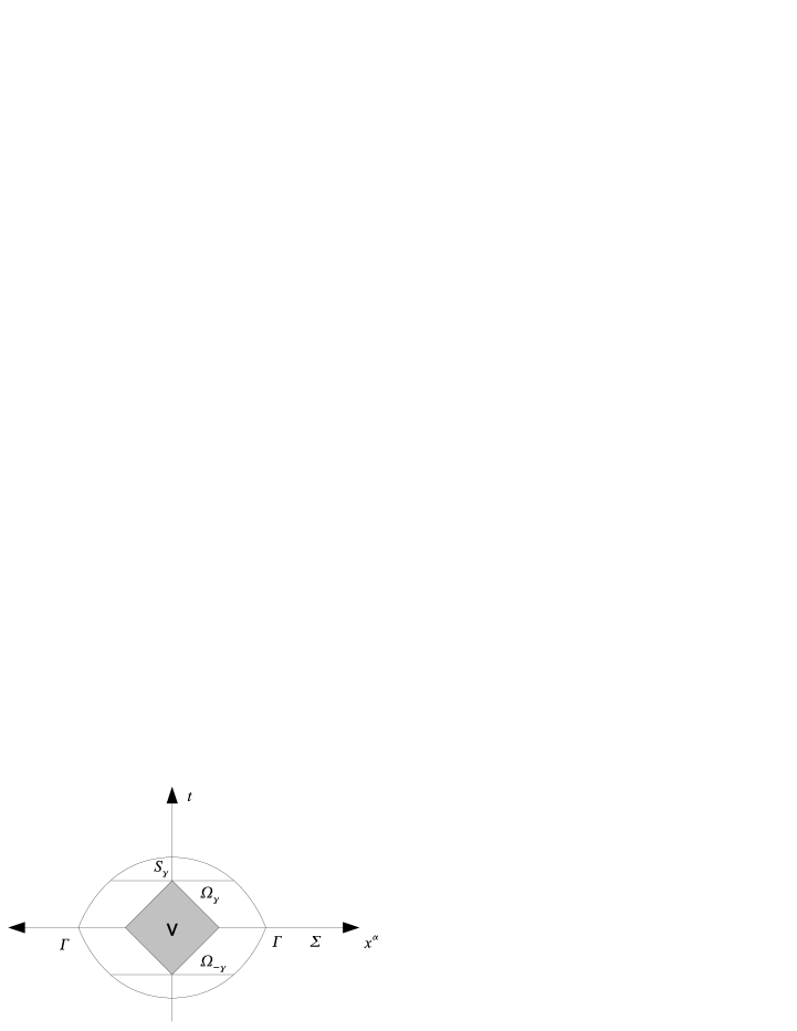
Figure 3.3. Choice of the open set $V$ for the existence result

We are now prepared to present the existence and uniqueness theorem for the Cauchy problem of the wave equation in our setting:

Theorem 3.36.

For each point $p$ in $\Sigma$ there exists an open neighborhood $V\subset U$ on which a unique generalized solution $u\in\mathcal{G}(V)$ of the initial value problem (3.23) exists.

Even though there will be redundancies, we shall present a detailed proof of the theorem.

Proof.

Let $(U,(t,x^{\mu}))$ be an open relatively compact static coordinate chart at $p$. By Theorem 3.16, we choose a representative $(g_{ab}^{\varepsilon})_{\varepsilon}$ of the metric which is static for each $\varepsilon$ and which (for small $\varepsilon$) satisfies the respective bounds according to the setting. Furthermore, a representative $(e_{ab}^{\varepsilon})_{\varepsilon}$ of $e_{ab}$ may be directly constructed from the representative $(g_{ab}^{\varepsilon})_{\varepsilon}$ of the metric.

Under these conditions Proposition 3.19 may be applied.

On the level of representatives the initial value problem (3.23) takes the form (3.24) with $(f_{\varepsilon})_{\varepsilon}$ negligible, and $(v_{\varepsilon})_{\varepsilon}$, $(w_{\varepsilon})_{\varepsilon}$ moderate.
Part 1. Existence of a local moderate net of solutions
The smooth theory then provides smooth solutions $(u_{\varepsilon})_{\varepsilon}$ on $U$.

We first show that the net $(u_{\varepsilon})_{\varepsilon}$ satisfies moderate bounds on $\Omega_{\gamma}$: Moderate data $(v_{\varepsilon})_{\varepsilon}$, $(w_{\varepsilon})_{\varepsilon}$ translate by means of Proposition 3.22 to moderate initial energies $(E^{k}_{0,\varepsilon}(u_{\varepsilon}))_{\varepsilon}$ for each hierarchy $k$. Moreover, by means of Proposition 3.32, moderate initial energies $(E^{k}_{0,\varepsilon}(u_{\varepsilon}))_{\varepsilon}$ ($k\geq 1$) translate to moderate energies $(E^{k}_{\tau,\varepsilon}(u_{\varepsilon}))_{\varepsilon}$ ($k\geq 1$), where $0\leq\tau\leq\gamma$, this is the statement of Proposition 3.33. Finally Proposition 3.35 states that moderate energies $(E^{k}_{\tau,\varepsilon}(u_{\varepsilon}))_{\varepsilon}$ ($k\geq 1,\,0\leq\tau\leq\gamma$) translate to moderate bounds of $(u_{\varepsilon})_{\varepsilon}$ and of its derivatives of all orders on $\Omega_{\gamma}$. Due to the preceding introductory remark, estimates of the same kind hold on $\Omega_{-\gamma}$. We pick an open subset $V$ of $\Omega_{-\gamma,\gamma}:=\Omega_{-\gamma}\cup\Omega_{\gamma}$ (see figure 3.3). Due to our considerations in the beginning of Part B (section 3.5), we have therefore established that $(u_{\varepsilon})_{\varepsilon}$ is a moderate net on $V$.
Part 2. Uniqueness of solutions
We may now define a local generalized solution $u$ on $V$ by

$$u:=[(u_{\varepsilon})_{\varepsilon}],$$

the class of $(u_{\varepsilon})_{\varepsilon}$ from Part 1. What is left to be shown is that the solution $u$ does not depend on the choice of representatives of $(f_{\varepsilon})_{\varepsilon},\,(v_{\varepsilon})_{\varepsilon},\,(w_{\varepsilon})_{\varepsilon}$ of $f\equiv 0,v,w$.

Let therefore $(\hat{f}_{\varepsilon})_{\varepsilon},\,(\hat{v}_{\varepsilon})_{\varepsilon},\,(\hat{w}_{\varepsilon})_{\varepsilon}$ be further representatives of $f\equiv 0,v,w$, and let $(\hat{u}_{\varepsilon})_{\varepsilon}$ be the respective net of smooth solutions.

Setting

$$\widetilde{u}_{\varepsilon}:=u_{\varepsilon}-\hat{u}_{\varepsilon},\;\widetilde{f}_{\varepsilon}:=f_{\varepsilon}-\hat{f}_{\varepsilon},\;\widetilde{v}_{\varepsilon}:=v_{\varepsilon}-\hat{v}_{\varepsilon},\;\widetilde{w}_{\varepsilon}:=w_{\varepsilon}-\hat{w}_{\varepsilon},$$

we see that for each $\varepsilon>0$ $\widetilde{u}_{\varepsilon}$ is a solution of the initial value problem

$$\Box^{\varepsilon}\widetilde{u}_{\varepsilon} = \widetilde{f}_{\varepsilon}$$

$$\widetilde{u}_{\varepsilon}(t=0,x^{\mu}) = \widetilde{v}_{\varepsilon}(x^{\mu})$$

$$\partial_{t}\widetilde{u}_{\varepsilon}(t=0,x^{\mu}) = \widetilde{w}_{\varepsilon}(x^{\mu}),$$

Note, that here all the nets $(\widetilde{f}_{\varepsilon})_{\varepsilon},(\widetilde{v}_{\varepsilon})_{\varepsilon},(\widetilde{w}_{\varepsilon})_{\varepsilon}$ are negligible. What is left to show is that the net $(\widetilde{u}_{\varepsilon})_{\varepsilon}$ is negligible, as well; uniqueness of the above defined solution $u$ is then obvious, since $[(\widetilde{u}_{\varepsilon})_{\varepsilon}]=[(u_{\varepsilon})_{\varepsilon}]=u$.

Negligible data $(v_{\varepsilon})_{\varepsilon}$, $(w_{\varepsilon})_{\varepsilon}$ translate by means of Proposition 3.22 to negligible initial energies $(E^{k}_{0,\varepsilon}(u_{\varepsilon}))_{\varepsilon}$ for each hierarchy $k$. Moreover, by means of Proposition 3.32, negligible initial energies $(E^{k}_{0,\varepsilon}(u_{\varepsilon}))_{\varepsilon}$ ($k\geq 1$) translate to negligible energies $(E^{k}_{\tau,\varepsilon}(u_{\varepsilon}))_{\varepsilon}$ ($k\geq 1$), where $0\leq\tau\leq\gamma$, this is the statement of Proposition 3.33. Finally Proposition 3.35 states that negligible energies $(E^{k}_{\tau,\varepsilon}(u_{\varepsilon}))_{\varepsilon}$ ($k\geq 1,\,0\leq\tau\leq\gamma$) translate to a negligible bounds of $(u_{\varepsilon})_{\varepsilon}$ and of its derivatives of all orders on $\Omega_{\gamma}$. Due to the preceding introductory remark, estimates of the same kind hold on $\Omega_{-\gamma}$. Due to our considerations in the beginning of Part B (section 3.5), we have therefore established that $(u_{\varepsilon})_{\varepsilon}$ is a negligible net on $V$. This proves uniqueness of the solution $u$ on $V$. ∎

3.10. Dependence on the representative of the metric (Part G)

So far, we have proved that on $V\subset\Omega_{\gamma}\cup\Omega_{-\gamma}$, a unique solution to the initial value problem exists. We had, however, picked a specific symmetric representative $(g_{ab}^{\varepsilon})_{\varepsilon}$ of the metric $g_{ab}$ (to be more precise, these are coordinate expressions of the metric components) and worked with one and the same all the time. It is, therefore, advisable, to show that the generalized solution $u$ of the wave equation is independent of the choice of the representative of the metric. This is the aim of this section.

There is only one further assumption we impose on the representatives $(g_{ab}^{\varepsilon})_{\varepsilon}$ of the metric: they shall be symmetric (cf. the note in the end of the section).

The initial value problem with respect to $(g_{ab}^{\varepsilon})_{\varepsilon}$ is the following:

(3.122) $$\Box^{\varepsilon}u_{\varepsilon} = f_{\varepsilon}$$

$$u_{\varepsilon}(t=0,x^{\alpha}) = v_{\varepsilon}(x^{\alpha})$$

$$\partial_{t}u_{\varepsilon}(t=0,x^{\alpha}) = w_{\varepsilon}(x^{\alpha})$$

Now, let $(\hat{g}_{ab}^{\varepsilon})_{\varepsilon}$ be another symmetric representative of $g_{ab}$. We call $\hat{\Box}^{\varepsilon}$ the
d’Alembertian operator induced by $(\hat{g}_{ab}^{\varepsilon})_{\varepsilon}$. The initial value problem with respect to the latter reads quite similarly

(3.123) $$\hat{\Box}^{\varepsilon}\hat{u}_{\varepsilon} = f_{\varepsilon}$$

$$\hat{u}_{\varepsilon}(t=0,x^{\alpha}) = v_{\varepsilon}(x^{\alpha})$$

$$\partial_{t}\hat{u}_{\varepsilon}(t=0,x^{\alpha}) = w_{\varepsilon}(x^{\alpha}).$$

We may pause here for a moment and consider why Proposition 3.19 (and therefore all subsequent statements based on the latter) also holds true for the alternative choice $(\hat{g}_{ab}^{\varepsilon})_{\varepsilon}$ of metric representative: First, the difference between $(\hat{g}_{ab}^{\varepsilon})_{\varepsilon}$ and the static representative $(g_{ab}^{\varepsilon})_{\varepsilon}$ (according to Theorem 3.16) is negligible by definition. As a consequence the difference between estimates established on compact sets and with respect to these different representative is negligible. Since we only work on the compact region $\Omega_{\gamma}$, the estimates according to Proposition 3.19 hold as well for other (symmetric) representatives of the metric and for small $\varepsilon$; however, presumably with modified positive constants $A,A^{\prime},B_{k},B_{k}^{\prime}$.

The proof of Theorem 3.36 (Part 1) provides moderate solutions $(u_{\varepsilon})_{\varepsilon}$ and $(\hat{u}_{\varepsilon})_{\varepsilon}$ of (3.122) and (3.123). It is only left to show that the difference $(\widetilde{u}_{\varepsilon})_{\varepsilon}:=(u_{\varepsilon})_{\varepsilon}-(\hat{u}_{\varepsilon})_{\varepsilon}$ is negligible on $\Omega_{\tau}$. For this difference we have

(3.124) $$\hat{\Box}^{\varepsilon}\widetilde{u}_{\varepsilon} = f_{\varepsilon}-\hat{\Box}^{\varepsilon}u_{\varepsilon}$$

$$\widetilde{u}_{\varepsilon}(t=0,x^{\alpha}) = 0$$

$$\partial_{t}\widetilde{u}_{\varepsilon}(t=0,x^{\alpha}) = 0.$$

In view of the proof of Theorem 3.36 (Part 2) we only need to show that $f_{\varepsilon}-\hat{\Box}^{\varepsilon}u_{\varepsilon}$ is negligible. To this end we first manipulate the right hand side of line 1 of (3.124) as follows:

(3.125) $$f_{\varepsilon}-\hat{\Box}^{\varepsilon}u_{\varepsilon}=(f_{\varepsilon}-\Box^{\varepsilon}u_{\varepsilon})+(\Box^{\varepsilon}u_{\varepsilon}-\hat{\Box}^{\varepsilon}u_{\varepsilon})=\Box^{\varepsilon}u_{\varepsilon}-\hat{\Box}^{\varepsilon}u_{\varepsilon},$$

because $(u_{\varepsilon})_{\varepsilon}$ solves (3.122). Therefore the problem is reduced to showing that $(\Box^{\varepsilon}u_{\varepsilon}-\hat{\Box}^{\varepsilon}u_{\varepsilon})_{\varepsilon}$ is negligible. We calculate the difference in local coordinates. We use $|\det g_{ij}^{\varepsilon}|:=|g_{\varepsilon}|=-g_{\varepsilon}$ and for the sake of simplicity we further omit the index $\varepsilon$. The difference then reads:

(3.126) $$\Box u-\hat{\Box}u=(-g)^{-\frac{1}{2}}\partial_{a}((-g)^{\frac{1}{2}}g^{ab}\partial_{b}u)-(-\hat{g})^{-\frac{1}{2}}\partial_{a}((-\hat{g})^{\frac{1}{2}}\hat{g}^{ab}\partial_{b}u)=$$

$$\left((-g)^{-\frac{1}{2}}\partial_{a}((-g)^{\frac{1}{2}}g^{ab}\partial_{b}u)-(-\hat{g})^{-\frac{1}{2}}\partial_{a}((-g)^{\frac{1}{2}}g^{ab}\partial_{b}u)\right)+$$

$$+\left((-\hat{g})^{-\frac{1}{2}}\partial_{a}((-g)^{\frac{1}{2}}g^{ab}\partial_{b}u)-(-\hat{g})^{-\frac{1}{2}}\partial_{a}((-\hat{g})^{\frac{1}{2}}\hat{g}^{ab}\partial_{b}u)\right)=$$

$$((-g)^{-\frac{1}{2}}-(-\hat{g})^{-\frac{1}{2}})\partial_{a}((-g)^{\frac{1}{2}}g^{ab}\partial_{b}u)+(-\hat{g})^{-\frac{1}{2}}\partial_{a}\left((-g)^{\frac{1}{2}}g^{ab}-(-\hat{g})^{\frac{1}{2}}\hat{g}^{ab}\right)\partial_{b}u$$

The differences within the brackets of the last line of (3.126) can easily be shown to be negligible. Indeed, since $(g_{ab}^{\varepsilon}-\hat{g}_{ab}^{\varepsilon})_{\varepsilon}$ is negligible, also $g_{\varepsilon}-\hat{g}_{\varepsilon}$ is negligible, therefore, as can be seen by the following elementary algebraic manipulation, the difference

(3.127) $$(-g_{\varepsilon})^{-\frac{1}{2}}-(-\hat{g}_{\varepsilon})^{-\frac{1}{2}}=\frac{g_{\varepsilon}-\hat{g}_{\varepsilon}}{\sqrt{g_{\varepsilon}\hat{g}_{\varepsilon}}(\sqrt{-\hat{g}_{\varepsilon}}+\sqrt{-g_{\varepsilon}})}$$

is negligible. Also

(3.128) $$\sqrt{-g_{\varepsilon}}g^{ab}-\sqrt{-\hat{g}_{\varepsilon}}\hat{g}^{ab}_{\varepsilon}=\sqrt{-g_{\varepsilon}}(g_{\varepsilon}^{ab}-\hat{g}_{\varepsilon}^{ab})+\hat{g}_{\varepsilon}^{ab}\frac{\hat{g}_{\varepsilon}-g_{\varepsilon}}{\sqrt{-g_{\varepsilon}}+\sqrt{-\hat{g}_{\varepsilon}}}$$

is negligible. Plugging (3.127) and (3.128) into (3.126), we derive that $(\Box^{\varepsilon}u_{\varepsilon}-\hat{\Box}^{\varepsilon}u_{\varepsilon})_{\varepsilon}$ is negligible, and by identity (3.125), $(f_{\varepsilon}-\hat{\Box}^{\varepsilon}u_{\varepsilon})_{\varepsilon}$ is a negligible net of smooth functions as well. This is the right hand side of the differential equation (3.124). Therefore, Part 2 of the proof of Theorem 3.36) ensures that $(\widetilde{u}_{\varepsilon})_{\varepsilon}=(u_{\varepsilon}-\hat{u}_{\varepsilon})_{\varepsilon}$ is negligible and we are done.

It goes without saying that non-symmetric perturbations of the metric are not relevant. Another formulation of the latter would be the following: The present method for solving the initial value problem (3.23) basically lies in showing the existence result on the level of representatives given an arbitrary choice of representatives of the initial data as a well as a symmetric representative of the metric. The resulting generalized solution does not depend on the choice of symmetric representatives of the metric and neither does it depend on the choice of representatives of the initial data.

3.11. Possible generalizations

We finish this chapter by pointing out possible improvements of Theorem 3.36 concerning generality of the statement as well as reducing the list of necessary assumption on the metric as given in section 3.3.2.

First we conjecture that condition (iv) in section 3.3.2, which guarantees existence of smooth solutions on the level of representatives (that is with respect to each sufficiently small $\varepsilon$–component of the representative of the metric), presumably follows from condition (i).

Moreover, we believe that the Cauchy problem (3.23) also admits unique solutions in the special algebra of generalized functions even if the condition (i) are weakened to logarithmic growth properties of the metric coefficients. In this case, the constants $A,A^{\prime},B_{k},B_{k}^{\prime}$ of Proposition 3.19 might depend on $\varepsilon$, say $A(\varepsilon)=A\log(\varepsilon)$ with a positive constant $A$ etc. . Therefore, a later application of Grownwall’s Lemma would yield moderate growth of energies of arbitrary order, since

$$(e^{A\log\varepsilon})_{\varepsilon}=(\varepsilon^{A})_{\varepsilon}$$

is moderate.

Chapter 4 Point values and uniqueness questions in algebras of generalized functions

4.1. Point value characterizations of ultrametric Egorov algebras

As already mentioned in the introduction, a distinguishing feature (compared to spaces of distributions in the sense of Schwartz) of Colombeau- and Egorov type algebras is the availability of a generalized point value characterization for elements of such spaces (see [38], resp. [30] for the manifold setting). Such a characterization may be viewed as a nonstandard aspect of the theory: for uniquely determining an element of a Colombeau- or Egorov algebra, its values on classical (’standard’) points do not suffice: there exist elements which vanish on each classical point yet are nonzero in the quotient algebra underlying the respective construction. A unique determination can only be attained by taking into account values on generalized points, themselves given as equivalence classes of standard points. This characteristic feature is re-encountered in practically all known variants of such algebras of generalized functions.

It therefore came as a surprise when in a series of papers ([2, 3]) it was claimed that, contrary to the above general situation, in $p$-adic Colombeau-Egorov algebras a general point value characterization using only standard points was available. This chapter is dedicated to a thorough study of (generalized) point value characterizations of $p$-adic Colombeau-Egorov algebras and to showing that in fact also in the $p$-adic setting classical point values do not suffice to uniquely determine elements of such.

In the remainder of this section we recall some material from ([2, 3]), using notation from [18]. Let $\mathbb{N}$ be the natural numbers starting with $n=1$. For a fixed prime $p$, let $\mathbb{Q}_{p}$ denote the field of rational $p$-adic numbers. Let $\mathcal{D}(\mathbb{Q}_{p}^{n})$ denote the linear space of locally constant complex valued functions on $\mathbb{Q}_{p}^{n}$ ($n\geq 1$) with compact support. Let further $\mathcal{P}(\mathbb{Q}_{p}^{n}):=\mathcal{D}(\mathbb{Q}_{p}^{n})^{\mathbb{N}}$. $\mathcal{P}(\mathbb{Q}_{p}^{n})$ is endowed with an algebra-structure by defining addition and multiplication of sequences component-wise. Let $\mathcal{N}(\mathbb{Q}_{p}^{n})$ be the subalgebra of elements $\{(f_{k})_{k}\}\in\mathcal{P}(\mathbb{Q}_{p}^{n})$ such that for any compact set $K\subseteq\mathbb{Q}_{p}^{n}$ there exists an $N\in\mathbb{N}$ such that $\forall\;x\in K\;\forall\;k\geq N:f_{k}(x)=0$. This is an ideal in $\mathcal{P}(\mathbb{Q}_{p}^{n})$. The quotient algebra $\mathcal{G}(\mathbb{Q}_{p}^{n}):=\mathcal{P}(\mathbb{Q}_{p}^{n})/\mathcal{N}(\mathbb{Q}_{p}^{n})$ is called the $p$-adic Colombeau-Egorov algebra. Finally, so called Colombeau-Egorov generalized numbers $\widetilde{\mathcal{C}}$ are introduced in the following way: Let $\bar{\mathbb{C}}$ be the one-point compactification of $\mathbb{C}\cup\{\infty\}$.
Factorizing $\mathcal{A}=\bar{\mathbb{C}}^{\mathbb{N}}$ by the ideal $\mathcal{I}:=\{u=(u_{k})_{k}\in\mathcal{A}\mid\,\exists N\in\mathbb{N}\,\forall\;k\geq N:u_{k}=0\}$ yields then the ring $\widetilde{\mathcal{C}}$ of Colombeau-Egorov generalized numbers. We replace $\bar{\mathbb{C}}$ by $\mathbb{C}$ and construct similarly $\mathcal{C}$, the ring of generalized numbers: Clearly, $\bar{\mathbb{C}}$ is not needed in this context, since representatives of elements $f\in\mathcal{G}(\mathbb{Q}_{p}^{n})$ merely take on values in $\mathbb{C}^{\mathbb{N}}$. Let $f=[(f_{k})_{k}]\in\mathcal{G}(\mathbb{Q}_{p}^{n})$. It is clear that for a fixed $x\in\mathbb{Q}_{p}^{n}$, the point value of f at x, $[(f_{k}(x))_{k}]$ is a well defined element of ${\mathcal{C}}$, i.e., we may consider $f$ as a map

(4.1) $$f:\;\mathbb{Q}_{p}^{n}\rightarrow\mathcal{C}:\;\;x\mapsto f(x):=(f_{k}(x))_{k}+\mathcal{I}.$$

Note that the above constitutes a slight abuse of notation: The letter $f$ denotes both a generalized function (an element of $\mathcal{G}(\mathbb{Q}_{p}^{n})$) and a mapping on $\mathbb{Q}_{p}^{n}$.
Finally, let $A$ be a set and let $R$ be a ring. For $B\subset A,\;\theta\in R$ we call the characteristic function of $B$ the map $\chi_{B,\theta}:\;A\rightarrow R$ which is identically $\theta$ on $B$ and which vanishes on $A\setminus B$. Furthermore, if $\theta=1\in R$ we simply write $\chi_{B}=\chi_{B,1}$.

4.1.1. Uniqueness via point values and a counterexample

The following statement is proved in Theorem 4.4 of [3]: Let $f\in\mathcal{G}(\mathbb{Q}_{p}^{n})$, then:

$$f=0\;\;\mbox{in}\;\;\mathcal{G}(\mathbb{Q}_{p}^{n})\Leftrightarrow\forall\;x\in\mathbb{Q}_{p}^{n}:f(x)=0\;\;\mbox{in}\;\;\mathcal{C}.$$

However, inspired by ([43], p. 218) we construct the following counterexample to this claim, which shows that point values cannot uniquely determine elements in $\mathcal{G}(\mathbb{Q}_{p}^{n})$ uniquely. For the sake of simplicity we assume that $n=1$.

Example 4.1.

For any $l\in\mathbb{N}$, set

$$B_{l}:=\{x\in\mathbb{Z}_{p}:|x-p^{l}|<|p^{2l}|\}\subset\{x\in\mathbb{Z}_{p}:|x|=|p^{l}|\}\,.$$

For any $i\in\mathbb{N}$, we set $f_{i}:=\chi_{B_{i}}$. Clearly $B_{i}\cap B_{j}=\emptyset$ whenever $i\neq j$ and since $f_{i}\in\mathcal{D}(\mathbb{Q}_{p})$ for all natural numbers $i$, $(f_{i})_{i}$ is a representative of some $f\in\mathcal{G}(\mathbb{Q}_{p})$. Now, for any $\alpha\in\mathbb{Q}_{p}$, $f(\alpha)=0$ in $\mathcal{C}$, since either $\alpha\in B_{i}$ for some $i\in\mathbb{N}$ (which implies that $f_{j}(\alpha)=0\;\forall\;j>i$) or $\alpha\in\mathbb{Q}_{p}\setminus\bigcup B_{i}$, where each $f_{i}$ ($i\in\mathbb{N}$) is identically zero. Consider now the sequence $(\beta_{i})_{i\geq 1}\in\mathbb{N}^{\mathbb{N}}\subseteq\mathbb{Z}_{p}^{\mathbb{N}}$, where $\beta_{i}=p^{i}\;\forall\;i\in\mathbb{N}$. It follows that $f_{i}(\beta_{i})=1\;\forall\;i\in\mathbb{N}$. In particular, for $K=\mathbb{Z}_{p}$ or any dressed ball containing $0$, there is no representative $(g_{j})_{j}$ of $f$ such that for some $N>0$, $g_{j}=0\;\forall\;j\geq N$. Hence $f\neq 0$ in $\mathcal{G}(\mathbb{Q}_{p})$ although all standard point values of $f$ vanish.

Remark 4.2.

By means of the above example we may analyze the proof of Theorem 4.4 in [3]. Let $f$ be the generalized function from 4.1. As a compact set choose $K:=B_{\leq p^{-2}}(0)=p^{2}\mathbb{Z}_{p}$. For the representative $(f_{k})_{k}$ constructed in 4.1 and $x=0$ we have $N(0)=1$, which in the notation of [3] means that for any $k\geq 1=N(0)$, $f_{k}(0)=0$. Also, recall that $B_{\gamma}(a)$ is the dressed ball $B_{\leq p^{\gamma}}(a)$. The “parameter of constancy” ([3], p. 6) of $f_{1}$ at $x=0$, which is the maximal $\gamma$ such that $f_{1}$ is identically zero on $B_{\gamma}(0)$, is $l_{0}(0)=-2$. Now, there exists a covering of $K$ consisting of a single set, namely $B_{l_{0}(0)}(0)$. Thus we may replace the application of the Heine-Borel Lemma in [3] by our singleton-covering. But then the claim that (4.1) and (4.2) imply that for all $k\geq N(0)=1$ we have $f_{k}(0+x^{\prime})=f_{k}(0)=0\;\forall\,x^{\prime}\in K$ does not hold. This indeed follows from the definition of the sequence $(f_{k})_{k}$ of locally constant functions from above, since for any $k\in\mathbb{N}$ we have $f_{k}(p^{k})=1$.

4.1.2. Egorov algebras on locally compact ultrametric spaces

In this section we investigate the problem of point value characterization in Egorov algebras in full generality: to this end we consider a general locally compact ultrametric space $(M,d)$ instead of $\mathbb{Q}_{p}^{n}$, where $M$ need not have a field structure. Our aim is to show that even in such a general setting, the respective algebra cannot have a point value characterization, unless $M$ carries the discrete topology. Denote by $\mathcal{E}_{d}(M)$ the algebra of sequences of locally constant functions with compact support, taking values in a commutative ring $R\neq\{0\}$. Let $\mathcal{N}_{d}(M)$ be the set of negligible functions $\{(f_{k})_{k}\}\in\mathcal{E}_{d}(M)$ such that for any compact set $K\subset M$ there exists an $N\in\mathbb{N}$ such that $\forall\;x\in K\;\forall\;k\geq N:f_{k}(x)=0$. The subset $\mathcal{N}_{d}(M)$ is an ideal in $\mathcal{E}_{d}(M)$ and the quotient algebra $\mathcal{G}(M,R):=\mathcal{E}_{d}(M)/\mathcal{N}_{d}(M)$ is called the ultrametric Egorov algebra associated with $(M,d)$. Furthermore, the ring of generalized numbers is defined by $\mathcal{R}:=R^{\mathbb{N}}/\sim$, where $\sim~{}$ is the equivalence relation on $R^{\mathbb{N}}$ given by

$$u\sim v\;\mbox{in}\;R^{\mathbb{N}}\Leftrightarrow\exists\,N\in\mathbb{N}\;\forall\;k\geq N:u_{k}-v_{k}=0.$$

We call $\mathcal{I}(R):=\{w\in R^{\mathbb{N}}:w\sim 0\}$ the ideal of negligible sequences in $R$. Analogous to (4.1), for $f\in\mathcal{G}(M,R)$ evaluation on standard point values is introduced by means of the mapping:

(4.2) $$f:\;M\rightarrow\mathcal{R}:\;\;x\mapsto f(x):=(f_{k}(x))_{k}+\mathcal{I}(R).$$

Definition 4.3.

An ultrametric Egorov algebra $\mathcal{G}(M,R)$ is said to admit a standard point value characterization if for each $u\in\mathcal{G}(M,R)$ we have

$$u=0\Leftrightarrow\forall\;x\in M:u(x)=0\;\mbox{in}\;\mathcal{R}.$$

Using this terminology, Example 4.1 shows that $\mathcal{G}(\mathbb{Q}_{p}^{n})$ does not admit a standard point value characterization. The main result of this section is the following generalization:

Theorem 4.4.

Let $(M,d)$ be a locally compact ultrametric space and let $R\neq\{0\}$. Then $\mathcal{G}(M,R)$ does not admit a standard point value characterization unless $(M,d)$ is discrete.

Proof.

The result follows by generalizing the construction of Example 4.1. Assume $(M,d)$ is not discrete, then there exists a point $x\in M$ and a sequence $(x_{n})_{n}$ of distinct points in $M$ converging to $x$. We may assume that $d(x,x_{i})>d(x,x_{j})$ whenever $i<j$. Define stripped balls $(B_{n})_{n\geq 1}$ with centers $(x_{n})_{n\geq 1}$ by $B_{n}:=\{y\in M\mid d(x_{n},y)<\frac{d(x_{n},x)}{2}\}$. Due to the ultrametric property “the strongest one wins” we have $B_{n}\subset\{z\mid d(x,z)=d(x_{n},x)\}$, which further implies that for all $i\neq j\;(i,\,j)\in\mathbb{N}$, the balls $B_{i}$, $B_{j}$ are disjoint sets in $M$. Since $R$ is a non-trivial ring, we may choose some $\theta\in R\setminus\{0\}$. Now we define a sequence $(f_{k})_{k}$ of locally constant functions in the following way: For any $i\geq 1$ set $f_{i}=\chi_{B_{i},\theta}$. Clearly, $f:=[(f_{i})_{i}]\in\mathcal{G}(M,R)$, and similarly to Example 4.1, for any $\alpha\in M$, $f(\alpha)=0$ in $\mathcal{R}$. Nevertheless for the sequence $(x_{n})_{n}$, which without loss of generality may be assumed to lie in a compact neighborhood of $x$, one has $f_{i}(x_{i})=\theta\;\forall\;i\geq 1$ which implies that $f\neq 0$ in $\mathcal{G}(M,R)$. ∎

Recall that a discrete topological space $X$ has the following properties:

1. $X$ is locally compact.

2. Any compact set in $X$ contains finitely many points only.

Therefore we know that for a set $D$ endowed with the discrete metric and for any commutative ring $R$, the respective ultrametric Egorov algebra $\mathcal{G}(D,R)$ admits a point wise characterization. We therefore conclude:

Corollary 4.5.

For a locally compact ultrametric space $(M,d)$ and a non-trivial ring $R$, the following statements are equivalent:

1. $\mathcal{G}(M,R)$ admits a standard point value characterization.

2. The topology of $(M,d)$ is discrete.

4.1.3. Generalized point values

In this section we give an appropriate generalized point value characterization in the style of ([38], pp. Theorem 2. 4) of $\mathcal{G}(M,R)$, where $M$ is endowed with a non-discrete ultrametric $d$ for which $M$ is locally compact, and $R\neq\{0\}$. First, we have to introduce a set $\widetilde{M}_{c}$ of compactly supported generalized points over $M$. Let $\mathcal{E}=M^{\mathbb{N}}$, the ring of sequences in $M$, and identify two sequences, if for some index $N\in\mathbb{N}$ one has $d(x_{n},y_{n})=0$ for each positive integer $n$, that is, $x_{n}=y_{n}\;\forall\;n\geq N$; we write $x\sim y$. We call $\widetilde{M}=\mathcal{E}/\sim$ the ring of generalized numbers. Finally, $\widetilde{M}_{c}$ is the subset of such elements $x\in\widetilde{M}$ for which there exists a compact subset $K$ and some representative $(x_{n})_{n}$ of $x$ such that for some $N>0$ we have $x_{n}\in K$ for all $n\geq N$. It follows that evaluating a function $u\in\mathcal{G}(M,R)$ at a compactly supported generalized point $x$ is possible, i.e., for representatives $(x_{k})_{k}$, $(u_{k})_{k}$ of $x$ resp.  $u$, $[(u_{k}(x_{k}))_{k}]$ is a well defined element of $\mathcal{R}$.

Proposition 4.6.

In $\mathcal{G}(M,R)$, there is a generalized point value characterization, i.e.,

$$u=0\;\mbox{in}\;\mathcal{G}(M,R)\;\Leftrightarrow\;\forall\;x\in\widetilde{M}_{c}:u(x)=0\;\;\mbox{in}\;\;\mathcal{R}.$$

Proof.

The condition on the right side obviously is necessary. Conversely, let $u\in\mathcal{G}(M,R)$, $u\neq 0$. This means that there is a representative $(u_{k})_{k}$ of $u$ and a compact set $K\subset\subset M$ such that $u_{k}$ does not vanish on $K$ for infinitely many $k\in\mathbb{N}$. In particular this means we have a sequence $(x_{k})_{k}$ in $K$ such that for infinitely many $k\in\mathbb{N}$, $u_{k}(x_{k})\neq 0$. Clearly this means that $u(x)\neq 0$ in $\mathcal{R}$, where we have set $x:=[(x_{k})_{k}]$. ∎

4.1.4. The $\delta$-distribution

In [3], Theorem 4.4 is illustrated by some examples, to highlight the advantage of a point value concept in $\mathcal{G}(\mathbb{Q}_{p}^{n})$. In this section we discuss the $\delta$-distribution (Example 4.5 on p. 12 in [3]) and construct a generalized function $f\in\mathcal{G}(\mathbb{Q}_{p})$ different from $\delta$ which however coincides with $\delta$ on all standard points in $\mathbb{Q}_{p}$. We first embed the $\delta$-distribution in $\mathcal{G}(\mathbb{Q}_{p})$ as in [3] (p. 9, Theorem 3.3) which yields $\iota(\delta)=(\delta_{k})_{k}+\mathcal{N}_{p}(\mathbb{Q}_{p})$, where $\delta_{k}(x):=p^{k}\Omega(p^{k}|x|_{p})$ for each $k$, and $\Omega$ is the bump function on $\mathbb{R}^{+}_{0}$ given by

$$\Omega(t):=\begin{cases}1,\;\;0\leq t\leq 1\\ 0,\;\;t>1\end{cases}.$$

Evaluation of $\iota(\delta)$ on standard points is shown in Example 4.5 of [3]. With $\tilde{c}:=(p^{k})_{k}+\mathcal{I}\in\mathcal{C}$ one has:

$$\iota(\delta)(x)=\begin{cases}\widetilde{c},\;\;x=0\\ 0,\;\;x\neq 0\end{cases}\qquad(x\in\mathbb{Q}_{p}).$$

Let $\varphi:\mathbb{N}\rightarrow\mathbb{Z}$ be a monotonous function such that $\lim_{k\rightarrow\infty}\varphi(k)=\infty$, and such that the cardinality of $U_{\varphi}:=\{k:\varphi(k)>k\}$ is infinite. Consider an element $f\in\mathcal{G}(\mathbb{Q}_{p})$ given by $f:=(f_{k})_{k}+\mathcal{N}(\mathbb{Q}_{p})$ where for any $k\geq 1$, $f_{k}(x):=p^{k}\Omega(p^{\varphi(k)}|x|_{p})$. Then the standard point values of $\iota(\delta)$ and $f$ coincide. Furthermore, they coincide on compactly supported generalized points $x\in\widetilde{\mathbb{Q}}_{p,c}$ with the property that for any representative $(x_{k})_{k}$ of $x$ there exists an $N\in\mathbb{N}$ such that $\forall\;k\geq N:\;|x_{k}|_{p}>p^{-\min\{k,\varphi(k)\}}$, since in this case we have $\delta_{k}(x_{k})=f_{k}(x_{k})=0$. However, there are compactly supported generalized points violating this condition which yield different generalized point values of $\iota(\delta)$ resp. $f$: for instance, take the generalized point $x_{0}:=[(p^{k})_{k}]\in\widetilde{\mathbb{Q}}_{p,c}$. Then $f(x_{0})\neq\widetilde{c}$, since $\theta_{k}:=f_{k}(x_{k})=0$ for any $k\in U_{\varphi}$ and thus $\theta_{k}=0$ for infinitely many $k\in\mathbb{N}$. But $\iota(\delta)(x_{0})=\widetilde{c}$.

4.2. Spherical completeness of the ring of generalized numbers

Let $(M,d)$ be an ultrametric space. For given $x\in M,r\in\mathbb{R}^{+}$, we call $B_{\leq r}(x):=\{y\in M\mid d(x,y)\leq r\}$ the dressed ball with center $x$ and radius $r$. Throughout $\mathbb{N}:=\{1,2,\dots\}$ denote the positive integers. Let $(x_{i})_{i}\in M^{\mathbb{N}}$ and $(r_{i})_{i}$ be a sequence of positive reals. We call $(B_{i})_{i},\;B_{i}:=B_{\leq r_{i}}(x_{i})\;(i\geq 1)$ a nested sequence of dressed balls, if $r_{1}\geq r_{2}\geq r_{3}\dots$ and $B_{1}\supseteq B_{2}\supseteq\dots$ . Following standard ultrametric literature (cf. [43]), nested sequences of dressed balls might have empty intersection. The converse property is defined as follows:

Definition 4.7.

$(M,d)$ is called spherically complete, if every nested sequence of dressed balls has a non-empty intersection.

It is evident that any spherically complete ultrametric space is complete with respect to the topology induced by its metric (using the well known fact that topological completeness of $(M,d)$ is equivalent to the property of Definition 4.7 with radii $r_{i}\searrow 0$) . However, there are popular non-trivial examples in the literature, for which the converse is not true. As an example we mention the field of complex $p$-adic numbers together with its $p$-adic valuation considered as the completion of the algebraic closure of the field $\mathbb{C}_{p}$ of rational $p$-adic numbers. Due to Krasner, this field has nice algebraic properties (as it is algebraically closed, and even isomorphic to the complex numbers cf. [43], pp. 134–145), but it also has been shown, that $\mathbb{C}_{p}$ is not spherically complete. This is mainly due to the fact that the complex $p$-adic numbers are a separable, complete ultrametric space with dense valuation (cf. [43], pp. 143–144). However, for an ultrametric field $K$, spherical completeness is necessary in order to ensure $K$ has the Hahn Banach extension property (to which we refer as HBEP), that is, any normed $K$-vector space $E$ admits continuous linear functionals previously defined on a strict subspace $V$ of $E$ to be extended to the whole space under conservation of their norm (cf. W. Ingleton’s proof [24]). Since spherical completeness fails, it is natural to ask if the $p$-adic numbers could at least be spherically completed, i.e., if there existed a spherically complete ultrametric field $\Omega$ into which $\mathbb{C}_{p}$ can be embedded. This question has a positive answer (cf. [43]). The necessity of spherical completeness for the HBEP of $K=\mathbb{C}_{p}$ is evident: even the identity map

$$\varphi:\;\;\mathbb{C}_{p}\rightarrow\mathbb{C}_{p},\quad\varphi(x):=x$$

cannot be extended to a functional $\psi:\Omega\rightarrow\mathbb{C}_{p}$ under conservation of its norm $\|\varphi\|=1$ (here we consider $\Omega$ as a $\mathbb{C}_{p}$- vector space).

The present work is motivated by the question if some version of Hahn-Banach’s Theorem holds on differential algebras in the sense of Colombeau considered as ultra pseudo normed modules over the ring of generalized numbers $\widetilde{\mathbb{R}}$ (resp. $\widetilde{\mathbb{C}}$). Even though topological questions on topological $\widetilde{\mathbb{C}}$ modules have been recently investigated to a wide extent (cf. C. Garetto’s recent papers [15, 16] as well as [11]), a HBEP has not yet been established in the literature.

The analogy with the $p$-adic case lies at hand, since the ring of generalized numbers can naturally be endowed with an ultrametric pseudo-norm. However, the presence of zero-divisor in $\widetilde{\mathbb{R}}$ as well as the failing multiplicativity of the pseudo-norm turns the question into a non-trivial one and Ingleton’s ultrametric version of the Hahn Banach Theorem cannot be carried over to our setting unrestrictedly.

On our first step tackling this question we discuss spherical completeness of the ring of generalized numbers endowed with the given ultrametric (induced by the respective pseudo-norm, cf. the preliminary section).

$\widetilde{\mathbb{R}}$ first was introduced as the set of values of generalized functions at standard points; however, a subring consisting of compactly supported generalized numbers turned out to be the set of points for which evaluation determines uniqueness, whereas standard points do not suffice do determine generalized functions uniquely (cf. [34, 38]). A hint, that $\widetilde{\mathbb{R}}$ (or $\widetilde{\mathbb{C}}$ as well), the ring of generalized real (or complex) numbers is spherically complete, is, that contrary to the above outlined situation on $\mathbb{C}_{p}$, the generalized numbers endowed with the topology induced by the sharp ultra-pseudo norm are not separable. This, for instance, follows from the fact that the restriction of the sharp valuation to the real (or complex) numbers is discrete.

Having motivated our work by now, we may formulate the aim of this section, which is to prove the following:

Theorem 4.8.

The ring of generalized numbers is spherically complete.

We therefore have an independent proof of the fact (cf. [16], Proposition 1. 30):

Corollary 4.9.

The ring of generalized numbers is topologically complete.

In the last section of this note we present a modified version of Hahn-Banach’s Theorem which bases on spherically completeness of $\widetilde{\mathbb{R}}$ (resp. $\widetilde{\mathbb{C}}$). Finally, a remark on the applicability of the ultra metric version of Banach fixed point theorem can be found in the Appendix.

4.2.1. Preliminaries

In what follows we repeat the definitions of the ring of (real or complex) generalized numbers along with its non-archimedean valuation function. The material is taken from different sources; as references we may recommend the recent works due to C. Garetto ([15, 16]) and A. Delcroix et al. ([11]) as well as one of the original sources of this topic due to D. Scarpalezos (cf. [12]).
Let $I:=(0,1]\subseteq\mathbb{R}$, and let $\mathbb{K}$ denote $\mathbb{R}$ resp. $\mathbb{C}$. The ring of generalized numbers over $\mathbb{K}$ is constructed in the following way: Given the ring of moderate (nets of) numbers

$$\mathcal{E}:=\{(x_{\varepsilon})_{\varepsilon}\in\mathbb{K}^{I}\mid\exists\;m:|x_{\varepsilon}|=O(\varepsilon^{m})\;(\varepsilon\rightarrow 0)\}$$

and, similarly, the ideal of negligible nets in $\mathcal{E}(\mathbb{K})$ which are of the form

$$\mathcal{N}:=\{(x_{\varepsilon})_{\varepsilon}\in\mathbb{K}^{I}\mid\forall\;m:|x_{\varepsilon}|=O(\varepsilon^{m})\;(\varepsilon\rightarrow 0)\},$$

we may define the generalized numbers as the factor ring $\widetilde{\mathbb{K}}:=\mathcal{E}_{M}/\mathcal{N}$. We define a (real valued) valuation function $\nu:$ on $\mathcal{E}_{M}(\mathbb{K})$ in the following way:

$$\nu((u_{\varepsilon})_{\varepsilon}):=\sup\,\{b\in\mathbb{R}\mid|u_{\varepsilon}|=O(\varepsilon^{b})\;\;(\varepsilon\rightarrow 0)\}.$$

This valuation can be carried over to the ring of generalized numbers in a well defined way, since for two representatives of a generalized number, the valuations above coincide (cf. [16], section 1). We then may endow $\widetilde{\mathbb{K}}$ with an ultra-pseudo-norm (’pseudo’ refers to non-multiplicativity) $|\;\;|_{e}$ in the following way: $|0|_{e}:=0$, and whenever $x\neq 0$, $|x|_{e}:=e^{-\nu(x)}$. With the metric $d_{e}$ induced by the above norm, $\widetilde{\mathbb{K}}$ turns out to be a non-discrete ultrametric space, with the following topological properties:

1. $(\widetilde{\mathbb{K}},d_{e})$ is topologically complete (cf. [16]),

2. $(\widetilde{\mathbb{K}},d_{e})$ is not separable, since the restriction of $d_{e}$ onto $\mathbb{K}$ is discrete.

The latter property holds, since on metric spaces second countability and separability are equivalent and the well known fact that the property of second countability is inherited by subspaces (whereas separability is not in general).

In order to avoid confusion we henceforth denote closed balls in $\mathbb{K}$ by $B_{\leq r}(x)$ in distinction with dressed balls in $\widetilde{\mathbb{K}}$ which we denote by $\widetilde{B}_{\leq r}(x)$. Similarly stripped balls and the sphere in the ring of generalized numbers are denoted by $\widetilde{B}_{<r}(x)$ resp. $\widetilde{S}_{r}(x)$.

4.2.2. Euclidean models of sharp neighborhoods

Throughout, a net of real numbers $(C_{\varepsilon})_{\varepsilon}$ is said to increase monotonously with $\varepsilon\rightarrow 0$, if the following holds:

$$\forall\eta,\eta^{\prime}\in I:\;(\eta\leq\eta^{\prime}\Rightarrow C_{\eta}\geq C_{\eta^{\prime}}).$$

To begin with we formulate the following condition:
Condition (E).
A net $(C_{\varepsilon})_{\varepsilon}$ of real numbers is said to satisfy condition (E), if it is

1. positive for each $\varepsilon$ and

2. monotonically increasing with $\varepsilon\rightarrow 0$, and finally, if

3. the sharp norm is $|(C_{\varepsilon})_{\varepsilon}|_{e}=1$.

Next, we introduce the notion of euclidean models of sharp neighborhoods of generalized points:

Definition 4.10.

Let $x\in\widetilde{\mathbb{K}}$, $\rho\in\mathbb{R},\;r:=\exp(-\rho)$. Let further $(C_{\varepsilon})_{\varepsilon}\in\mathbb{R}^{I}$ be a net of real numbers satisfying condition (E) and let $(x_{\varepsilon})_{\varepsilon}$ be a representative of $x$. Then we call the net of closed balls $(B_{\varepsilon})_{\varepsilon}\subseteq\mathbb{K}^{I}$ given by

$$B_{\varepsilon}:=B_{\leq C_{\varepsilon}\varepsilon^{\rho}}(x_{\varepsilon})$$

for each $\varepsilon\in I$ an euclidean model of $\widetilde{B}(x,r)$.

Note, that every dressed ball admits an euclidean model: let $(x_{\varepsilon})_{\varepsilon}$ be a representative of $x$ and define $(C_{\varepsilon})_{\varepsilon}$ by $C_{\varepsilon}:=1$ for each $\varepsilon\in I$; then $B_{\leq C_{\varepsilon}\varepsilon^{\rho}}(x_{\varepsilon})$ yields determines an euclidean model of $\widetilde{B}_{\leq r}(x)$.
We need to mention that whenever we write $(B^{(1)}_{\varepsilon})_{\varepsilon}\subseteq(B^{(2)}_{\varepsilon})_{\varepsilon}$, we mean the inclusion relation $\subseteq$ holds component wise (that is for each $\varepsilon\in I$), and we say $(B^{(2)}_{\varepsilon})_{\varepsilon}$ contains $(B^{(1)}_{\varepsilon})_{\varepsilon}$.
The following lemma is basic; however, in order to get familiar with the concept of euclidean neighborhoods, we include a detailed proof:

Lemma 4.11.

For $x\in\widetilde{\mathbb{K}},r>0$, let $(B_{\varepsilon})_{\varepsilon}$ be an euclidean model for $\widetilde{B}_{\leq r}(x)$ and set$\rho=-\log r$. Then we have:

1. Any $y\in\widetilde{B}_{<r}(x)$ has a representative $(y_{\varepsilon})_{\varepsilon}$ such that $y_{\varepsilon}\in B_{\varepsilon}$ for each $\varepsilon\in I$.

2. There exist $y\in\widetilde{S}_{r}(x):=\{x^{\prime}\in\widetilde{\mathbb{K}}:|x^{\prime}-x|=r\}$ which cannot be caught by representatives lying in $(B_{\varepsilon})_{\varepsilon}$. However one may blow $(B_{\varepsilon})_{\varepsilon}$ always up to a new model $(\hat{B}_{\varepsilon})_{\varepsilon}$ which contains some representative of $y$, i.e., there exists a net $(D_{\varepsilon})_{\varepsilon}$ satisfying Condition (E) such that for $\hat{C}_{\varepsilon}:=C_{\varepsilon}D_{\varepsilon}$, $\hat{B}_{\varepsilon}:=B_{\leq\hat{C}_{\varepsilon}\varepsilon^{\rho}}(x_{\varepsilon})$ yields a model containing some representative of $y$

3. In any case, it can be arranged, that $d(\partial\hat{B}_{\varepsilon},y_{\varepsilon})\geq\frac{C_{\varepsilon}}{2}\varepsilon^{\rho}$ for each $\varepsilon\in I$, for some model $(\hat{B}_{\varepsilon})_{\varepsilon}$ of $\widetilde{B}_{\leq r}(x)$ containing $(B_{\varepsilon})_{\varepsilon}$.

Proof.

(i): By definition of the sharp norm, $|y-x|_{e}<r$ is equivalent to the situation, that for each representative $(y_{\varepsilon})_{\varepsilon}$ of $y$ and for each representative $(x_{\varepsilon})_{\varepsilon}$ of $x$, we have

$$\sup\{b\in\mathbb{R}\mid|y_{\varepsilon}-x_{\varepsilon}|=O(\varepsilon^{b})(\varepsilon\rightarrow 0)\}>\rho,$$

and this implies that there exists some $\rho^{\prime}>\rho$ such that for any representative $(y_{\varepsilon})_{\varepsilon}$ of $y$ and any representative $(x_{\varepsilon})_{\varepsilon}$ of $x$ we have

$$|y_{\varepsilon}-x_{\varepsilon}|=o({\varepsilon}^{\rho^{\prime}}),\quad\varepsilon\rightarrow 0.$$

This further implies that for any choice of representatives of $x$ resp. of $y$, there exists some $\eta\in I$ with

(4.3) $$|y_{\varepsilon}-x_{\varepsilon}|\leq\varepsilon^{\rho^{\prime}}$$

for each $\varepsilon<\eta$. Since $C_{\varepsilon}>0$ for each $\varepsilon\in I$ and $C_{\varepsilon}$ is monotonously increasing with $\varepsilon\rightarrow 0$, we have $\varepsilon^{\rho^{\prime}}\leq C_{\varepsilon}\varepsilon^{\rho}$ for sufficiently small $\varepsilon$, therefore, a suitable choice of $y_{\varepsilon}$, for $\varepsilon\geq\eta$, yields the first claim (for instance, one may set $y_{\varepsilon}:=x_{\varepsilon}$ whenever $\varepsilon\geq\eta$).
We go on by proving (ii): For the first part, set

$$y_{\varepsilon}:=2C_{\varepsilon}\varepsilon^{\rho}+x_{\varepsilon}$$

Let $y$ denote the class of $(y_{\varepsilon})_{\varepsilon}$. It is evident, that $y\in\widetilde{B}_{\leq r}(x)$. However, $(y_{\varepsilon})\notin B_{\varepsilon}$ for each $\varepsilon\in I$. Indeed,

$$\forall\;\varepsilon\in I:|y_{\varepsilon}-x_{\varepsilon}|=2C_{\varepsilon}\varepsilon^{\rho}>C_{\varepsilon}\varepsilon^{\rho},$$

since $C_{\varepsilon}>0$ for each $\varepsilon$. We further show, that the same holds for any representative $(\bar{y}_{\varepsilon})_{\varepsilon}$ of $y$ for sufficiently small index $\varepsilon$. Indeed, the difference of two representatives being negligible implies that for any $N>0$ we have

$$y_{\varepsilon}-\hat{y}_{\varepsilon}=o(\varepsilon^{N})\;\;(\varepsilon\rightarrow 0).$$

Therefore, for $N>\rho$ and sufficiently small $\varepsilon$, we have:

$$|\hat{y}_{\varepsilon}-y_{\varepsilon}|\geq||\hat{y}_{\varepsilon}-y_{\varepsilon}|-|y_{\varepsilon}-x_{\varepsilon}||\geq 2C_{\varepsilon}\varepsilon^{\rho}-\varepsilon^{N}\geq\frac{3}{2}C_{\varepsilon}\varepsilon^{\rho}>C_{\varepsilon}\varepsilon^{\rho}.$$

Therefore we have shown the first part of (ii). Let $y\in\widetilde{S}_{r}(x)$. We demonstrate how to blow up $(B_{\varepsilon})_{\varepsilon}$ to catch some fixed representative $(y_{\varepsilon})_{\varepsilon}$ of $y$. Since $|y-x|=e^{-\rho}=r$, there is a net $C^{\prime}_{\varepsilon}\geq 0$ ($|(C^{\prime}_{\varepsilon})_{\varepsilon}|_{e}=1$) such that

$$\forall\varepsilon\in I:\;|y_{\varepsilon}-x_{\varepsilon}|=C_{\varepsilon}^{\prime}\varepsilon^{\rho}$$

Set $C^{\prime\prime}_{\varepsilon}=\max_{\eta\geq\varepsilon}\{1,C^{\prime}_{\eta}\}$. This ensures that $(C^{\prime\prime}_{\varepsilon})$ is a monotonously increasing with $\varepsilon\rightarrow 0$, above $1$ for each $\varepsilon\in I$, and $|(C^{\prime\prime}_{\varepsilon})|_{e}=1$ is preserved. Define $B^{\prime}_{\varepsilon}:=B_{\leq C_{\varepsilon}C^{\prime\prime}_{\varepsilon}\varepsilon^{\rho}}(x_{\varepsilon})$. Then $(B^{\prime}_{\varepsilon})_{\varepsilon}$ is a new model for $\widetilde{B}_{\leq r}(x)$ containing the old model and $(y_{\varepsilon})_{\varepsilon}$ as well, since the product $C_{\varepsilon}C^{\prime\prime}_{\varepsilon}$ has the required properties, and

$$|y_{\varepsilon}-x_{\varepsilon}|\leq C^{\prime\prime}_{\varepsilon}\varepsilon^{\rho}\leq C_{\varepsilon}^{\prime\prime}C_{\varepsilon}\varepsilon^{\rho}$$

and we are done with (ii).
Proof of (iii): So far, we have shown that for each $y\in\widetilde{B}_{\leq r}(x)$, there exists an euclidean model $(B_{\leq C_{\varepsilon}\varepsilon^{\rho}}(x_{\varepsilon}))$ of $B_{\leq r}(x)$ such that for some representative $(y_{\varepsilon})_{\varepsilon}$ of $y\in\widetilde{B}_{\leq r}(x)$ we have

$$\forall\;\varepsilon\in I:y_{\varepsilon}\in B_{\varepsilon}.$$

Therefore, by replacing $C_{\varepsilon}$ by $2C_{\varepsilon}$ above, again a model for $\widetilde{B}_{\leq r}(x)$ is achieved, however with the further property that $|y_{\varepsilon}-x_{\varepsilon}|\leq C_{\varepsilon}/2\varepsilon^{\rho}$ for each $\varepsilon\in I$ which proves our claim.∎

Before going on by establishing the crucial statement which will allow us to translate decreasing sequences of closed balls in the given ultrametric space $\widetilde{\mathbb{K}}$ to decreasing sequences of their (appropriately chosen) euclidean models, we introduce a useful term:

Definition 4.12.

Suppose, we have a nested sequence $(\widetilde{B}_{i})_{i=1}^{\infty}$ of closed balls with centers $x_{i}$ and radius $r_{i}$ in $\widetilde{\mathbb{K}}$ and for each $i\in\mathbb{N}$ we have an euclidean model $(B^{(i)}_{\varepsilon})_{\varepsilon}$. We say, this associated sequence of euclidean models is proper, if $\left((B^{(i)}_{\varepsilon})_{\varepsilon}\right)_{i=1}^{\infty}$ is nested as well, that is, if we have:

$$(B^{(1)}_{\varepsilon})_{\varepsilon}\supseteq(B^{(2)}_{\varepsilon})_{\varepsilon}\supseteq(B^{(3)}_{\varepsilon})_{\varepsilon}\supseteq\dots.$$

4.2.3. Proof of the main theorem

In order to prove the main statement, we proceed by establishing two important preliminary statements. First, a remark on the notation in the sequel: If $(x_{i})_{i}$, a sequence of points in the ring of generalized numbers, is considered, then $(x_{\varepsilon}^{(i)})_{\varepsilon}$ denote (certain) representatives of the $x_{i}$’s. Furthermore, for subsequent choices of nets of real numbers $(C^{(i)}_{\varepsilon})_{\varepsilon}$, and positive radii $r_{i}$, we denote by $\rho_{i}$ the negative logarithms of the $r_{i}$’s ($i=1,2,\dots,$) and the euclidean models of the balls $\widetilde{B}_{\leq r_{i}}(x_{i})$ with radii $r_{\varepsilon}^{i}:=C_{\varepsilon}^{(i)}\varepsilon^{\rho_{i}}$ to be constructed are denoted by

$$B_{\varepsilon}^{(i)}:=B_{\leq r_{\varepsilon}^{(i)}}(x_{\varepsilon}^{(i)}).$$

We start with the fundamental proposition:

Proposition 4.13.

Let $x_{1},\;x_{2}\in\widetilde{\mathbb{K}}$, and $r_{1},\;r_{2}$ be positive numbers such that $\widetilde{B}_{\leq r_{1}}(x_{1})\supseteq\widetilde{B}_{\leq r_{2}}(x_{2})$. Let $(x^{(1)}_{\varepsilon})_{\varepsilon}$ be a representative of $x_{1}$. Then the following holds:

1. There exists a net $(C^{(1)}_{\varepsilon})_{\varepsilon}$ satisfying condition (E) such that for each $\varepsilon\in I$

   (4.4) $$x_{\varepsilon}^{(2)}\in B_{\leq\frac{C_{\varepsilon}^{(1)}\varepsilon^{\rho_{1}}}{2}}(x_{\varepsilon}^{(1)}).$$

2. Furthermore, for each net $(C^{(2)}_{\varepsilon})_{\varepsilon}$ satisfying condition (E) there exists an $\varepsilon_{0}^{(1)}\in I$ such that for each $\varepsilon<\varepsilon_{0}^{(1)}\in I$ we have $B^{(2)}_{\varepsilon}\subseteq B^{(1)}_{\varepsilon}$.

Proof.

Proof of (i): Let $(x_{\varepsilon}^{(2)})_{\varepsilon}$ be a representative of $x_{1}$. We distinguish the following two cases:

1. $x_{2}\in\widetilde{S}_{r_{1}}(x_{1})$, that is, $|x_{2}-x_{1}|_{e}=r_{1}$. Let $(x_{\varepsilon}^{(2)})_{\varepsilon}$ be a representative of $x_{2}$. Define $\hat{C}_{\varepsilon}^{(1)}:=|x_{\varepsilon}^{(1)}-x_{\varepsilon}^{(2)}|$. Now, set $C_{\varepsilon}^{(1)}:=2\max(\{\hat{C}_{\eta}^{(1)}|\eta>\varepsilon\},1)$. Then not only $C_{\varepsilon}^{(1)}>0$ for each parameter $\varepsilon$, but also the net $C_{\varepsilon}^{(1)}>0$ is monotonically increasing with $\varepsilon\rightarrow 0$, furthermore (4.4) holds, and we are done with this case.

2. $x_{2}\notin\widetilde{S}_{r_{1}}(x_{1})$, that is, $|x_{2}-x_{1}|_{e}<r_{1}$. Set, for instance, $C_{\varepsilon}^{(1)}=1$. For each representative $(x_{\varepsilon}^{(2)})_{\varepsilon}$ of $x_{2}$ it follows that

   $$|x_{\varepsilon}^{(2)}-x_{\varepsilon}^{(1)}|=o(\varepsilon^{\rho_{1}})$$

   and a representative satisfying the desired properties is easily found.

Proof of (ii):
To show this we consider the asymptotic growth of $(C_{\varepsilon}^{(1)})_{\varepsilon},(C_{\varepsilon}^{(2)})_{\varepsilon},\varepsilon^{\rho_{1}},\varepsilon^{\rho_{2}}$ as well as the monotonicity of $C_{\varepsilon}^{(1)}$: let $y\in B_{\leq C_{\varepsilon}^{(2)}\varepsilon^{\rho_{2}}}(x_{\varepsilon}^{(2)})$. Then we have by the triangle inequality for each $\varepsilon\in I$:

(4.5) $$|y-x_{\varepsilon}^{(1)}|\leq|y-x_{\varepsilon}^{(2)}|+|x_{\varepsilon}^{(2)}-x_{\varepsilon}^{(1)}|\leq C_{\varepsilon}^{(2)}\varepsilon^{\rho_{2}}+\frac{C_{\varepsilon}^{(1)}\varepsilon^{\rho_{1}}}{2}.$$

We know further that by the monotonicity $\forall\varepsilon\in I:C_{\varepsilon}^{(1)}\geq C_{0}^{(1)}:=C_{0}$ so that

(4.6) $$\frac{C_{\varepsilon}^{(2)}}{C_{\varepsilon}^{(1)}}\varepsilon^{\rho_{2}-\rho_{1}}\leq C_{0}C_{\varepsilon}^{(2)}\varepsilon^{\rho_{2}-\rho_{1}}.$$

Moreover, since the sharp norm of $C_{\varepsilon}^{(2)}$ equals $1$, for any $\alpha>0$ we have

$$C_{\varepsilon}^{(2)}=o(\varepsilon^{-\alpha}),\;(\varepsilon\rightarrow 0).$$

which in conjunction with the fact that $\rho_{2}>\rho_{1}$ allows us to further estimate the right hand side of (4.6): Obtaining

$$\frac{C_{\varepsilon}^{(2)}}{C_{\varepsilon}^{(1)}}\varepsilon^{\rho_{2}-\rho_{1}}=o(1),\;(\varepsilon\rightarrow 0),$$

we plug this information into (4.5). This yields for sufficiently small $\varepsilon$, say $\varepsilon<\varepsilon_{0}^{(1)}$:

(4.7) $$|y-x_{\varepsilon}^{(1)}|\leq\frac{C_{\varepsilon}^{(1)}\varepsilon^{\rho_{1}}}{2}+\frac{C_{\varepsilon}^{(1)}\varepsilon^{\rho_{1}}}{2}=C_{\varepsilon}^{(1)}\varepsilon^{\rho_{1}};$$

the proof is finished. ∎

Proposition 4.14.

Any nested sequence of closed balls in $\widetilde{\mathbb{K}}$ admits a proper sequence of associated euclidean models.

Proof.

We proceed step by step so that we may easily read off the inductive argument of the proof in the end.
We may assume that for each $i\geq 1$, $r_{i}>r_{i+1}$. Define $\rho_{i}:=-\log(r_{i})$ (so that $\rho_{i}<\rho_{i+1}$ for each $i\geq 1$).
Step 1.
Choose a representative $(x^{(1)}_{\varepsilon})_{\varepsilon}$ of $x_{1}$.
Step 2.
Due to Proposition 4.13 (i) we may choose a representative $(x^{(2)}_{\varepsilon})_{\varepsilon}$ of $x_{2}$ and a net $(C^{(1)}_{\varepsilon})_{\varepsilon}$ of real numbers satisfying condition (E) such that such that for each $\varepsilon\in I$

$$x_{\varepsilon}^{(2)}\in B_{\leq\frac{C_{\varepsilon}^{(1)}\varepsilon^{\rho_{1}}}{2}}(x_{\varepsilon}^{(1)}).$$

Denote by $\varepsilon_{0}^{(1)}\in I$ be the maximal $\varepsilon$ such that the inclusion relation $B^{(2)}_{\varepsilon}\subseteq B^{(1)}_{\varepsilon}$ as in (cf. (ii) of Proposition 4.13) holds.
Step 3.
Similarly, take a representative $(\hat{x}^{(3)}_{\varepsilon})_{\varepsilon}$ of $x_{3}$ and a net $(\hat{C}^{(2)}_{\varepsilon})_{\varepsilon}$ of real numbers satisfying condition (E) such that such that for each $\varepsilon\in I$

(4.8) $$\hat{x}_{\varepsilon}^{(3)}\in B_{\leq\frac{\hat{C}_{\varepsilon}^{(2)}\varepsilon^{\rho_{2}}}{2}}(x_{\varepsilon}^{(2)}).$$

We show now, how to adjust our choice of $\hat{x}_{\varepsilon}^{(3)},\hat{C}_{\varepsilon}^{(2)}$ such that condition (E) as well as the inclusion relation (4.8) is preserved, however, we do this in a way such that we moreover achieve the inclusion relation

(4.9) $$B^{(2)}_{\varepsilon}\subseteq B^{(1)}_{\varepsilon}$$

for each $\varepsilon$ (for sufficiently small parameter this is guaranteed by the proceeding proposition).
For $\varepsilon\geq\varepsilon_{0}^{(1)}$ we leave the choice unchanged, that is, we set

$$x_{\varepsilon}^{(3)}:=\hat{x}_{\varepsilon}^{(3)},\;C_{\varepsilon}^{(2)}:=\hat{C}_{\varepsilon}^{(2)};$$

for $\varepsilon<\varepsilon_{0}^{(1)}$, however, we set

(4.10) $$x_{\varepsilon}^{(3)}:=x_{\varepsilon}^{(2)},\;C_{\varepsilon}^{(2)}:=\min(\frac{C_{\varepsilon}^{(1)}}{2}\varepsilon^{\rho_{1}-\rho_{2}},\hat{C}_{\varepsilon}^{(2)}).$$

Therefore, $(C_{\varepsilon}^{(2)})_{\varepsilon}$ still satisfies condition (E), since it is still positive and monotonically increasing with $\varepsilon\rightarrow 0$, furthermore we have only modified for big parameter $\varepsilon$, the asymptotic growth with $\varepsilon\rightarrow 0$ therefore remains unchanged (and so does the sharp norm of $(C_{\varepsilon}^{(2)})_{\varepsilon}$, which it is identically $1$). Next, it is evident that

$$x_{\varepsilon}^{(3)}\in B_{\leq\frac{C_{\varepsilon}^{(2)}\varepsilon^{\rho_{2}}}{2}}(x_{\varepsilon}^{(2)}).$$

still holds for each $\varepsilon\in I$. Finally, by (4.10) it follows that the inclusion relation (4.9) holds now for each $\varepsilon\in I$. For the inductive proof of the statement one formally proceeds as in Step 3. Let $k>1$. Assume we have representatives

$$(x_{\varepsilon}^{(1)})_{\varepsilon},\dots,(x_{\varepsilon}^{(k+1)})_{\varepsilon}$$

and nets of positive numbers

$$(C_{\varepsilon}^{(j)})_{\varepsilon},(1\leq j\leq k),$$

satisfying condition (E), such that for each $\varepsilon\in I$ we have:

$$B_{\leq C_{\varepsilon}^{(1)}\varepsilon^{\rho_{1}}}(x_{\varepsilon}^{(1)})\supseteq B_{\leq C_{\varepsilon}^{(2)}\varepsilon^{\rho_{2}}}(x_{\varepsilon}^{(2)})\supseteq\dots\supseteq B_{\leq C_{\varepsilon}^{(k-1)}\varepsilon^{\rho_{k-1}}}(x_{\varepsilon}^{(k-1)}).$$

and for some $\varepsilon_{0}^{(k-1)}$ we have for each $\varepsilon<\varepsilon_{0}^{(k-1)}$

$$B_{\leq C_{\varepsilon}^{(k-1)}\varepsilon^{\rho_{k-1}}}(x_{\varepsilon}^{(k-1)})\supseteq B_{\leq C_{\varepsilon}^{(k)}\varepsilon^{\rho_{k}}}(x_{\varepsilon}^{(k)}).$$

Furthermore we suppose the following additional property is satisfied: For each $\varepsilon\in I$ we have:

$$x_{\varepsilon}^{(k+1)}\in B_{\leq\frac{C_{\varepsilon}^{(k)}}{2}\varepsilon^{\rho_{k}}}(x_{\varepsilon}^{(k)}),$$

where $\rho_{k}:=-\log r_{k}$. In the very same manner as above, we may now find a representative $(x_{\varepsilon}^{(k+2)})_{\varepsilon}$ of $x_{k+2}$ and a net of numbers $(C_{\varepsilon}^{(k+1)})_{\varepsilon}$ satisfying condition (E) such that the above sequential construction can be enlarged by one ($k\rightarrow k+1$). ∎

The preceding proposition is a key ingredient in the proof of our main statement Theorem 4.8:

Proof.

Let $(\widetilde{B}_{i})_{i=1}^{\infty},\;B_{i}:=\widetilde{B}_{\leq r_{i}}(x_{i})\;(i\geq 1)$ be the given nested sequence of dressed balls; due to Proposition 4.14, there exists a proper sequence of associated euclidean models

$$(B^{(i)}_{\varepsilon})_{\varepsilon}$$

such that for representatives $(x^{(i)}_{\varepsilon})_{\varepsilon}$ of $x_{i}$ ($i\geq 1$) the above nets are given by

$$B^{(i)}_{\varepsilon}:=B_{\leq C_{\varepsilon}^{(i)}\varepsilon^{\rho_{i}}}(x^{(i)}_{\varepsilon}),\quad\rho_{i}:=-\log r_{i},\quad C_{\varepsilon}^{(i)}\in\mathbb{R}_{+}$$

for each $(\varepsilon,i)\in I\times\mathbb{N}$. Since $\mathbb{K}$ is locally compact, for each $\varepsilon\in I$ we may choose some $x_{\varepsilon}\in\mathbb{R}$ such that

$$x_{\varepsilon}\in\bigcap_{i=1}^{\infty}B^{(i)}_{\varepsilon}$$

since for each $\varepsilon\in I$ we have $B_{\varepsilon}^{(1)}\supseteq B_{\varepsilon}^{(2)}\supseteq\dots$. Since the sequence of euclidean models of the $\widetilde{B}_{i}$’s is proper, for each $\varepsilon\in I$ further holds:

$$|x_{\varepsilon}-x_{\varepsilon}^{(i)}|\leq C_{\varepsilon}^{(i)}\varepsilon^{\rho_{i}}.$$

This shows that not only the net $(x_{\varepsilon})_{\varepsilon}$ is moderate (use the triangle inequality), but also gives rise to a generalized number $x:=(x_{\varepsilon})_{\varepsilon}+\mathcal{N}(\mathbb{K})$ with the property

$$|x-x_{i}|_{e}\leq r_{i}$$

for each $i$. This shows that

$$x\in\bigcap_{i=1}^{\infty}\widetilde{B}_{i}\neq\emptyset$$

which yields the claim: $\widetilde{\mathbb{K}}$ is spherically complete. ∎

4.2.4. A Hahn-Banach Theorem

Let $L$ be a subfield of $\widetilde{\mathbb{K}}$ such that $\nu_{e}$ restricted to $L$ is additive. Let $E$ be an ultra pseudo-normed $L$-linear space. We call $\varphi$ an $L$- linear functional on $E$, if $\varphi$ is an $L$- linear mapping on $E$ with values in $\widetilde{\mathbb{K}}$. $\varphi$ is continuous if

$$\|\varphi\|:=\sup_{0\neq x\in E}\frac{|\varphi(x)|}{\|x\|}<\infty$$

and the space of all continuous $L$-linear functionals on $E$ we denote by $E^{\prime}_{L}$.

Remark 4.15.

Note that nontrivial subfields $L$ of $\widetilde{\mathbb{K}}$ exist. For instance, one may choose $\mathbb{K}(\alpha)$ with $\alpha=[(\varepsilon)_{\varepsilon}]\in\widetilde{\mathbb{K}}$ or its completion with respect to $|\;\;|_{e}$-the Laurent series over $\widetilde{\mathbb{K}}$.

Having introduced these notions we show that following version of the Hahn-Banach Theorem holds:

Theorem 4.16.

Let $V$ be an $L$-linear subspace of $E$ and $\varphi\in V^{\prime}_{L}$. Then $\varphi$ can be extended to some $\psi\in E^{\prime}_{L}$ such that $\|\psi\|=\|\varphi\|$.

Proof.

We follow the lines of the proof of Ingleton’s theorem (cf. [24]) in the fashion of ([43], pp. 194–195). To start with, let $V$ be a strict $L$-linear subspace of $E$ and let $a\in E\setminus V$. We first show that $\varphi\in V^{\prime}_{L}$ can be extended to $\psi\in(V+La)^{\prime}_{L}$ under conservation of its norm. To do this it is sufficient to prove that such $\psi$ satisfies for each $x\in V$:

(4.11) $$\|\psi(x-a)\| \leq \|\psi\|\cdot\|x-a\|$$

$$\|\varphi(x)-\psi(a)\| \leq \|\varphi\|\cdot\|x-a\|=:r_{x}.$$

To this end define for each $x$ in $V$ the dressed ball

$$B_{x}:=B_{\leq r_{x}}(\varphi(x)).$$

Next we claim that the family $\{B_{x}\mid x\in V\}$ of dressed balls is nested. To see this, let $x,y\in V$. By the linearity of $\varphi$ and the ultrametric (strong) triangle inequality we have

$$|\varphi(x)-\varphi(y)|\leq\|\varphi\|\cdot\|x-y\|\leq\|\varphi\|\max(\|x-a\|,\|y-a\|)=\max(r_{x},r_{y}).$$

Therefore we have $B_{x}\subseteq B_{y}$ or $B_{y}\subseteq B_{x}$ or vice versa. According to Theorem 4.8, $\widetilde{\mathbb{K}}$ is spherically complete, therefore we may choose

$$\alpha\in\bigcap_{x\in V}B_{x}$$

and further define $\psi(a):=\alpha$. Due to (4.11) and the homogeneity of the sharp norm with respect to the field $L$ we therefore have for each $z\in V$ and for each $\lambda\in L$,

$$|\psi(z-\lambda a)|=|\lambda|\cdot|\psi(z/\lambda-a)|\leq|\lambda|r_{z/\lambda}=|\lambda|\|\varphi\|\cdot\|z/\lambda-a\|=\|\varphi\|\cdot\|z-\lambda a\|$$

which shows that $\psi$ is an extension of $\varphi$ onto $V+La$ and $\|\psi\|=\|\varphi\|$.

The rest of the proof is the standard one-an application of Zorn’s Lemma. ∎

Let $E$ be a ultra pseudo-normed $\widetilde{\mathbb{K}}$ module and denote by $E^{\prime}$ all continuous linear functionals on $E$. We end this section by posing the following conjecture:

Conjecture 4.17.

Let $V$ be a submodule of $E$ and let $\varphi\in V^{\prime}$. Then $\varphi$ can be extended to some element $\psi\in E^{\prime}$ such that $\|\psi\|=\|\varphi\|$.

Appendix

Finally, it is worth mentioning that apart from the standard Fixed Point Theorem due to Banach, a non-archimedean version is available in spherically complete ultrametric spaces ( therefore, also on $\widetilde{\mathbb{K}}$, cf. [41], and for a recent generalization cf. [42]):

Theorem 4.18.

Let ($M,d$) be a spherically complete ultrametric space and $f:M\rightarrow M$ be a mapping having the property

$$\forall x,y\in M:d(f(x),f(y))<d(x,y).$$

Then $f$ has a unique fixed point in $M$.

4.3. Scaling invariance in algebras of generalized functions

Recent research in the field of generalized functions increasingly focuses on intrinsic problems in algebras of generalized functions. This is emphasized by a number of scientific papers on algebraic (cf. [5]) and topological topics (cf. [11, 12, 15, 16]).

In this chapter we investigate scaling invariance of generalized functions. We prove that a generalized function on the real line which is invariant under positive standard scaling has to be a constant. Also, we add a couple of further new characterizations of locally constant generalized functions to the well known ones. Our proof is partially based on the solution of the so-called ”Lobster problem”. It was at the International Conference on Generalized functions 2000 (April, 17–21) that Professor Michael Oberguggenberger offered a lobster for the answer to the question: ”Are generalized functions which are invariant under standard translations, merely the constants?” A (positive) answer to the latter was first given by S. Pilipovic, D. Scarpalezos and V. Valmorin in [40] and an independent proof has recently been established by H. Vernaeve [48].

Note that there is also an evident link between the present work and that of S. Konjik and M. Kunzinger dealing with group invariants in algebras of generalized functions ([25, 26]) which are also partially based on the solution of the Lobster problem.

4.3.1. Preliminaries

The setting of this chapter is the special algebra $\mathcal{G}(\mathbb{R}^{d})$ of generalized functions (cf. the introduction).

To start with we shortly review the specific concepts resp. methods we are going to employ in the sequel: association and integration of generalized functions, generalized points and sharp topology as well as continuity issues with respect to the latter. For the sake of simplicity we set $d=1$. For the generalized point value concept in algebras of generalized functions introduced by M. Kunzinger and M. Oberguggenberger in [38], we refer to the introduction. Next, let us recall the so-called sharp topology on the ring of generalized numbers:

The sharp topology on $\widetilde{\mathbb{R}}$

The - maybe most natural - topology on the ring of generalized numbers is the one which respects the asymptotic growth by means of which they are defined. Define a (real valued) valuation function $\nu$ on $\mathcal{E}_{M}(\mathbb{R})$ in the following way:

$$\nu((u_{\varepsilon})_{\varepsilon}):=\sup\,\{b\in\mathbb{R}\mid|u_{\varepsilon}|=O(\varepsilon^{b})\;\;(\varepsilon\rightarrow 0)\}.$$

This valuation can be carried over to the ring of generalized numbers in a well defined way, since for two representatives of a generalized number, their valuations coincide (cf. [16], chapter 1). We then may endow $\widetilde{\mathbb{R}}$ with an ultra-pseudo-norm (’pseudo’ refers to non-multiplicativity) $|\;\;|_{e}$ in the following way: $|0|_{e}:=0$, and whenever $x\neq 0$, $|x|_{e}:=e^{-\nu(x)}$. With the metric $d_{e}$ induced by the above norm, $\widetilde{\mathbb{R}}$ turns out to be a non-discrete ultrametric space, with the following topological properties:

1. $(\widetilde{\mathbb{R}},d_{e})$ is topologically complete (cf. [16]),

2. $(\widetilde{\mathbb{R}},d_{e})$ is not separable, since the restriction of $d_{e}$ onto $\mathbb{R}$ is discrete.

The latter property holds, since on metric spaces second countability and separability are equivalent and the well known fact that the property of second countability is inherited by subspaces (whereas separability is not in general).

Continuity issues

In ([4]) Aragona et al. develop a new concept of differentiability of generalized functions $f$ viewed as maps $\widetilde{f}:\widetilde{\mathbb{R}}_{c}\rightarrow\widetilde{\mathbb{R}}$, a concept which is compatible with partial differentiation in $\mathcal{G}(\mathbb{R}^{d})$ and evaluation of functions at generalized points. We need not recall this in detail; we only mention one notable consequence which we will make use of subsequently:

Fact 4.19.

If $\widetilde{f}:\widetilde{\mathbb{R}}_{c}\rightarrow\widetilde{\mathbb{R}}$ is induced by a generalized function, then $\widetilde{f}$ is continuous with respect to the sharp topology on $\widetilde{\mathbb{R}}_{c}$.

Integration of generalized functions

Generalized functions may be integrated over relatively compact Lebesgue measurable sets. We recall an elementary statement (this is Proposition 1.2.56 in [18]):

Fact 4.20.

Let $M$ be a Lebesgue-measurable set such that $\bar{M}\subset\subset\mathbb{R}$ and take $u\in\mathcal{G}(\mathbb{R})$. Let $(u_{\varepsilon})_{\varepsilon}$ be a representative of $u$. Then

$$\int_{M}u(x)dx:=\left(\int_{M}u_{\varepsilon}(x)\,dx\right)_{\varepsilon}+\mathcal{N}$$

is a well-defined element of $\widetilde{\mathbb{R}}$ called the integral of $u$ over $M$.

Also, we are going to need the ’antiderivative’ $F$ of a generalized function. Let $f\in\mathcal{G}(\mathbb{R})$. This we introduce by

$$F(x):=\int_{0}^{x}f(s)ds:=\left(\int_{0}^{x}f_{\varepsilon}(s)ds\right)_{\varepsilon}+\mathcal{N}(\mathbb{R})\in\mathcal{G}(\mathbb{R})$$

where $(f_{\varepsilon})_{\varepsilon}$ is an arbitrary representative of $f$. Note that $F$ is the primitive of $f$ with point value $F(0)=0$ in $\widetilde{\mathbb{R}}$ (cf. Proposition 1.2.58 in [18]).

The concept of association

Finally we recall the concept of association in $\widetilde{\mathbb{R}}$ and in $\mathcal{G}(\mathbb{R}^{d})$. First, let $\alpha\in\widetilde{\mathbb{R}}$. We write $\alpha\approx 0$ and we say ”$\alpha$ is associated to zero”, if for some (hence any) representative $(\alpha_{\varepsilon})_{\varepsilon}$ we have

$$\alpha_{\varepsilon}\rightarrow 0\qquad\mbox{whenever}\qquad\varepsilon\rightarrow 0.$$

Similarly, we say $u\in\mathcal{G}(\mathbb{R}^{n})$ is associated with zero, if for each test function $\phi$ we have

$$\int u_{\varepsilon}(x)\phi(x)\,dx^{n}\rightarrow 0\qquad\mbox{whenever}\qquad\varepsilon\rightarrow 0.$$

The relation $\approx$ is an equivalence relation on $\widetilde{\mathbb{R}}$ resp. $\mathcal{G}(\mathbb{R}^{d})$. By slightly abusing the above terminology we write $u\approx w$, $w\in\mathcal{D}^{\prime}(\mathbb{R}^{d})$ and say ”$u$ is associated with $w$” (or , ”$w$ is the distributional shadow of $u$”), if we have

$$\int u_{\varepsilon}(x)\phi(x)\,dx^{n}\rightarrow\langle w,\phi\rangle\qquad\mbox{whenever}\qquad\varepsilon\rightarrow 0.$$

It is a well known fact that a generalized function $u$ has at most one distributional shadow (cf. [18], Proposition 1.2.67).

4.3.2. Generalized functions supported at the origin

To start with we establish a basic lemma:

Lemma 4.21.

Let $f\in\mathcal{G}(\mathbb{R})$ be a non-negative function with $\mathop{\mathrm{supp}}(f)\subseteq\{0\}$. If for some $a>0$ we have

$$I(f)=\int_{[-a,a]}f(x)dx=0,$$

then $f=0$.

Proof.

We present two variants of the proof:
First Proof.
It has been shown recently (cf. [37]) that if for a generalized function $f$ we have for all $\varphi\in\mathcal{G}_{c}(\mathbb{R})$ (the space of compactly supported generalized functions)

$$\int f(x)\varphi(x)\,dx=0,$$

then $f=0$ in $\mathcal{G}(\mathbb{R})$. This is the so-called fundamental lemma of the calculus of variations in the generalized context. Now we have by the non-negativity of $f$,

$$\left|\int f(x)\varphi(x)\,dx\right|\leq\|\varphi\|_{\infty}\int f(x)dx=0,$$

therefore by the above we have $f=0$ in $\mathcal{G}(\mathbb{R})$ and we are done.
Alternative Proof.
This proof employs continuity arguments of generalized functions with respect to the sharp topology. In view of the first proof this may also yield a link between the fundamental lemma of variational calculus (in the generalized setting) and (sharp) topological issues. For our (indirect) proof we proceed in three steps.
Step 1.
Since $f$ is non-negative and $K:=[-a,a]\subset\subset\mathbb{R}$ is a compact set, we may choose a representative $(f_{\varepsilon})_{\varepsilon}$ of $f$ which is non-negative on $K$, that is, $(f_{\varepsilon})_{\varepsilon}$ satisfies:

$$\forall\;x\in K\;\forall\;\varepsilon>0:f_{\varepsilon}\geq 0.$$

Assume $f\neq 0$ in $\mathcal{G}(\mathbb{R})$. Due to (cf. subsection 1.2), there exists a compactly supported generalized point $x_{c}\in\widetilde{\mathbb{R}}$ such that $f(x_{c})=c\neq 0$. From our assumption on the support of $f$ ($\mathop{\mathrm{supp}}(f)\subseteq\{0\}$) it is further evident that $x_{c}\approx 0$; this information, however, is not crucial for what follows).
Step 2.
Let $(x_{\varepsilon})_{\varepsilon}$ be a representative of $x_{c}$. We shall prove the following:

(4.12) $$\exists\;\varepsilon_{k}\rightarrow 0\;\exists\;m_{0}\;\exists\;\rho_{0}\;\forall\;k\;\forall\;y_{k}\in[x_{\varepsilon_{k}}-\varepsilon_{k}^{\rho_{0}},x_{\varepsilon_{k}}+\varepsilon_{k}^{\rho_{0}}]:f_{\varepsilon_{k}}(y_{k})\geq\varepsilon_{k}^{m_{0}}.$$

To see this, we first observe by means of Step 1 that there exists a zero sequence $\varepsilon_{k}$ and a real number $m_{0}$ such that for each $k\geq 0$ we have $f_{\varepsilon_{k}}(x_{\varepsilon_{k}})\geq 2\varepsilon_{k}^{m_{0}}$ (we shall take this zero sequence as the one of our claim). Next, we employ a continuity argument to prove (4.12). Recall that $f$ viewed as a map $\widetilde{f}:\widetilde{\mathbb{R}}_{c}\rightarrow\widetilde{\mathbb{R}}$ is continuous with respect to the sharp topology (cf. subsection 4.3.1). Assume that (4.12) is not true. Then for each $m$ and for each $\rho$ there exists a sequence $(y_{k})_{k}$ with $y_{k}\in[x_{\varepsilon_{k}}-\varepsilon_{k}^{\rho},x_{\varepsilon_{k}}+\varepsilon_{k}^{\rho}]$ for each $k$ such that

(4.13) $$0\leq f_{\varepsilon_{k}}(y_{k})<\varepsilon_{k}^{m}$$

(the first inequality holds because we may assume without loss of generality that everything takes place inside $[-a,a]$, where we have found a non-negative representative of $f$). Define a (compactly supported) generalized number $y:=(y_{\varepsilon})_{\varepsilon}+\mathcal{N}$ via

$$y_{\varepsilon}:=\begin{cases}y_{k},\quad\mbox{if}\;\varepsilon=\varepsilon_{k}\\ x_{\varepsilon},\quad\mbox{otherwise}\end{cases}$$

Then we have for sufficiently small $m$

$$|f_{\varepsilon_{k}}(x_{\varepsilon_{k}})-f_{\varepsilon_{k}}(y_{\varepsilon_{k}})|>2\varepsilon_{k}^{m_{0}}-\varepsilon_{k}^{m}>\varepsilon_{k}^{m_{0}},$$

whereas for $\varepsilon\neq\varepsilon_{k}$ we have by the above construction that $f_{\varepsilon}(x_{\varepsilon})-f_{\varepsilon}(y_{\varepsilon})=0$ . In terms of the sharp norm $|\;\;|_{e}$ we therefore have:

$$|f(x_{c})-f(y)|_{e}\geq e^{-m_{0}};$$

by our assumption, however, it follows that

$$|x_{c}-y|_{e}\leq e^{-\rho_{0}}.$$

The choice of $\rho$ was arbitrary, and $\rho\rightarrow 0$ violates the continuity of $f$ at $x_{c}$. Therefore we have established (4.12). This we apply in the third and final step:
Step 3.
For sufficiently large $k$ we obtain

(4.14) $$\int_{[-a,a]}f_{\varepsilon_{k}}(y)dy>\varepsilon_{k}^{m_{0}}(2\varepsilon_{k}^{\rho})=2\varepsilon_{k}^{\rho+m_{0}}.$$

Since $\left(\int_{[-a,a]}f_{\varepsilon}(y)dy\right)_{\varepsilon}$ is a representative of $I(f)$, inequality (4.14) contradicts our assumption $I(f)=0$ (the representative not being a negligible net) and we are done. ∎

A further ingredient in the subsequent proof of our main result is the elementary observation that generalized scaling invariant functions $f\in\mathcal{G}(\mathbb{R})$ with support contained in the origin have to be identically zero. To motivate our proof, we first analyze the-maybe- simplest non-trivial example: a generalized function $\hat{\rho}$ associated with a distribution supported at the origin, say $\delta$. In this situation invariance under standard scaling is absurd: Assume we are given a standard mollifier $\rho\in C_{c}^{\infty}(\mathbb{R})$, that is $\int_{\mathbb{R}}\rho(x)dx=1$. Then $\rho_{\varepsilon}:(\frac{1}{\varepsilon}\rho(\frac{x}{\varepsilon}))_{\varepsilon}$ gives rise to a generalized function $\hat{\rho}:=[(\rho_{\varepsilon})_{\varepsilon}]\in\mathcal{G}(\mathbb{R})$ and, as it is well known, we have:

$$\hat{\rho}\approx\delta,\quad\mbox{that is,}\quad\forall\varphi\in\mathcal{C}_{c}^{\infty}(\mathbb{R}):\;\lim_{\varepsilon\rightarrow 0}\langle\rho_{\varepsilon},\varphi\rangle\rightarrow\langle\delta,\varphi\rangle=\varphi(0).$$

Consider now, $h\neq 0,1$ and assume the identity $\hat{\rho}(hx)=\hat{\rho}(x)$ holds in $\mathcal{G}(\mathbb{R})$. This in particular means that

$$\hat{\rho}=[(\rho_{\varepsilon}(hx))_{\varepsilon}]\qquad\mbox{in}\qquad\mathcal{G}(\mathbb{R})$$

holds as well. But for each $\varphi\in\mathcal{C}_{c}^{\infty}(\mathbb{R}),\;\varphi(0)\neq 0$ we have

$$\lim_{\varepsilon\rightarrow 0}\langle\rho_{\varepsilon}(hx),\varphi(x)\rangle\rightarrow\frac{1}{h}\varphi(0)\neq\langle\delta,\varphi\rangle$$

therefore $\hat{\rho}$ has more than one distributional shadow, namely $\delta,h\delta,\;$ for arbitrary $h\neq 0$ which is impossible! We may now present the statement in full generality:

Proposition 4.22.

Assume $f\in\mathcal{G}(\mathbb{R})$ has the following properties:

1. $f$ is invariant under positive standard scaling.

2. $\mathop{\mathrm{supp}}(f)\subseteq\{0\}$.

Then $f=0$ in $\mathcal{G}(\mathbb{R})$.

Proof.

Assume $f\in\mathcal{G}(\mathbb{R})$ satisfies the assumption of the proposition and without loss of generality we further assume $f\geq 0$ (otherwise, take $f^{2}$ instead of $f$). Let $(f_{\varepsilon})_{\varepsilon}$ be a representative of $f$ and $a>0$. Since $f$ is supported at the origin, the integral

$$I(f):=\int_{[-a,a]}f(x)dx:=\left(\int_{[-a,a]}f_{\varepsilon}(x)dx\right)_{\varepsilon}+\mathcal{N}\in\widetilde{\mathbb{R}}$$

is well defined, that is, the value $I(f)$ is independent of the choice of $a>0$ resp. of the representative of $f$. Further, for each $h\neq 0,1$ and each $\varepsilon>0$ we have:

$$\int_{[-a,a]}f_{\varepsilon}(xh)dx=\frac{1}{h}\int_{[-ah,ah]}f_{\varepsilon}(s)ds.$$

The scaling invariance of $f$, therefore, which in terms of representatives reads

$$(f_{\varepsilon}(x))_{\varepsilon}-(f_{\varepsilon}(hx))_{\varepsilon}=(n_{\varepsilon}(x))_{\varepsilon}\in\mathcal{N}(\mathbb{R}),$$

combined with the fact that $f$ is supported in the origin, yields

$$I(f)=\frac{1}{h}I(f)\qquad\mbox{in}\qquad\widetilde{\mathbb{R}}.$$

Since $h\neq 0,1$ this implies $I(f)=0$. Now we may apply Lemma 4.21 to the non-negative function $f$, and we obtain $f=0$. ∎

4.3.3. The main theorem

We are now ready to state the main theorem:

Theorem 4.23.

Let $f\in\mathcal{G}(\mathbb{R})$. The following are equivalent:

1. $f$ is constant, that is, there exists an $a\in\widetilde{\mathbb{R}}$ such that $f=a$ holds in $\mathcal{G}(\mathbb{R})$.

2. $\widetilde{f}$ is constant.

3. $\widetilde{f}$ is locally constant.

4. $f$ is translation invariant, that is $\forall h\in\mathbb{R}:f(x+h)=f(x)$ holds in $\mathcal{G}(\mathbb{R})$.

5. $f$ is invariant under positive standard scaling, that is,

   $$\forall h\in\mathbb{R}^{+}:f(hx)=f(x).$$

6. $F$ is additive, that is, $\forall h\in\mathbb{R}:F(x+h)=F(x)+F(h)$ holds in $\mathcal{G}(\mathbb{R})$.

7. $\widetilde{F}$ is additive, that is,

   $$\forall x_{c},h_{c}\in\widetilde{\mathbb{R}}:\widetilde{F}(x_{c}+h_{c})=\widetilde{F}(x_{c})+\widetilde{F}(h_{c})$$

   holds in $\widetilde{\mathbb{R}}$.

8. $F$ has the following property: There exists $\gamma\in(0,1)$ such that the identity:

   (4.15) $$\forall h\in\mathbb{R}:F(\gamma x+(1-\gamma)h)=\gamma F(x)+(1-\gamma)F(h)$$

   holds in $\mathcal{G}(\mathbb{R})$.

Proof.

We establish the implications (iii)$\Rightarrow$(i)$\Rightarrow$(ii)$\Rightarrow$(iii) as well as
(viii)$\Rightarrow$(iv)$\Rightarrow$(i)$\Rightarrow$(viii) and the equivalences (i)$\Leftrightarrow$(vi), (i)$\Leftrightarrow$(v), To begin with, assume (iii), that is $f$ is locally constant. We show the implication by applying the generalized differential calculus for Colombeau generalized functions evaluated on generalized points as has been developed by Aragona et al. in ([4]). Let $\kappa:\mathcal{G}(\mathbb{R})\rightarrow\widetilde{\mathbb{R}}^{\widetilde{\mathbb{R}}_{c}}$ be the linear embedding of generalized functions into mappings on compactly supported points due to [38]. Due to ([4], Theorem 4.1) differentiation in $\mathcal{G}(\mathbb{R})$ resp. in $\widetilde{\mathbb{R}}^{\widetilde{\mathbb{R}}_{c}}$ commute with $\kappa$. Clearly $\kappa(f)$ is differentiable with derivative $\kappa(f)^{\prime}\equiv 0$, and as just mentioned, $\kappa(f^{\prime})=\kappa(f)^{\prime}=0$, therefore, due to the generalized point characterization in $\mathcal{G}(\mathbb{R})$ ([38]) we have $f^{\prime}=0$ in $\mathcal{G}(\mathbb{R})$ and integrating yields (i) that is, $f$ is constant as a generalized function. The latter immediately implies (ii) by evaluating $f$ on compactly supported generalized numbers and the implication (ii)$\Rightarrow$(iii) is trivial.
Next, let $\gamma\in(0,1)$ and assume (4.15) holds for $F$. Differentiating yields

$$\forall h\in\mathbb{R}:f(\gamma x+(1-\gamma)h)=f(x)\quad\mbox{holds in}\quad\mathcal{G}(\mathbb{R}).$$

This is equivalent to

(4.16) $$\forall h\in\mathbb{R}:f(x+h)=f(\gamma^{-1}x)\quad\mbox{holds in}\quad\mathcal{G}(\mathbb{R}).$$

Setting $h=0$ shows that $f(x)=f(\gamma^{-1}x)$ in $\mathcal{G}(\mathbb{R})$ which further implies

(4.17) $$\forall h\in\mathbb{R}:f(x+h)=f(x)\quad\mbox{holds in}\quad\mathcal{G}(\mathbb{R}),$$

i. e., $f$ is translation invariant. This proves (iv). The implication (iv)$\Rightarrow$(i) is proven in ([40], Theorem 6); for an alternative proof cf. the appendix to [48]. Since $f=a$ implies $F=ax$ in $\mathcal{G}(\mathbb{R})$, the implication (i)$\Rightarrow$(viii) holds.
Further we establish the equivalence (i)$\Leftrightarrow$(vi). Again (i) implies that $F$ is of the form $F=ax$ with some generalized number $a$, therefore (vi) holds. Conversely, assume that f satisfies

$$F(x+h)=F(x)+F(h)\quad\mbox{holds in}\quad\mathcal{G}(\mathbb{R})$$

for each $h\in\mathbb{R}$. Differentiation yields

$$\forall h\in\mathbb{R}:f(x+h)=f(x)\quad\mbox{holds in}\quad\mathcal{G}(\mathbb{R})$$

and by the above this implies (i). Finally we establish the equivalence (i)$\Leftrightarrow$(v). Since (i)$\Rightarrow$(v) is trivial, we only need to show (i)$\Leftarrow$(v):
Note that without loss of generality we may assume that $f$ is symmetric (or equivalently, $f$ is invariant under any non-zero standard scaling). Indeed, if $f$ is not, we may introduce the two functions $g_{\pm}$ resp. $f_{\pm}$ given via

$$g_{+}(x):=f_{+}^{2}(x):=(f(x)+f(-x))^{2},\quad g_{-}(x):=f_{-}^{2}(x):=(f(x)-f(-x))^{2}.$$

If for generalized constants $c_{1},c_{2}$ we would have $g_{+}=c_{1},g_{-}=c_{2}$, then for some generalized constants $d_{1},d_{2}$ we would have $f_{+}=d_{1},f_{-}=d_{2}$, therefore

$$f(x):=\frac{f_{+}(x)+f_{-}(x)}{2}=\frac{d_{1}+d_{2}}{2},$$

that is, $f$ is a constant, and we would be done.
We may proceed now in two different ways: the first is a variant of H. Vernaeve’s ([48]) proof of the Lobster problem.
First proof.
We distinguish the two possible cases, ’$f$ is constant in a neighborhood of $1$’ or not.
Case 1
Assume first, there exist a neighborhood $\Omega:=(1-\delta,1+\delta)$ of $1$, $\delta>0$ and $c\in\widetilde{\mathbb{R}}$ such that $f=c$ on $\Omega$. Since $f$ is invariant under positive standard scaling and symmetric, it follows that

1. For each $h>0$, $f=c$ on $(h-h\delta,h+h\delta)$.

2. $f(x)=f(-x)$ in $\mathcal{G}(\mathbb{R})$.

Since $\mathcal{G}(\mathbb{R})$ is a sheaf, $f=c$ on $\mathbb{R}\setminus\{0\}$ and we have obtained a scaling invariant generalized function $g:=f-c$ with $\mathop{\mathrm{supp}}(g)\subseteq\{0\}$. Applying Proposition 4.22 yields $g=0$, that is, $f$ is a constant and we are done with the first case.
Case 2
If $f|_{\Omega}\in\mathcal{G}(\Omega)$ is non-constant on every standard neighborhood $\Omega=(1-\delta,1+\delta)$ ($\delta>0$) of $1$, then we have for any representative $(f_{\varepsilon})_{\varepsilon}$ of $f$:

$$(f_{\varepsilon}|_{\Omega}-f_{\varepsilon}(1))\notin\mathcal{N}(\Omega).$$

Thus there exists a representative $(f_{\varepsilon})_{\varepsilon}$ of $f$ along with a zero sequence $(\varepsilon_{k})_{k}$, a sequence $(a_{k})_{k}\in[\frac{1}{2},\frac{3}{2}]^{\mathbb{N}}$ and an $N$ such that for all sufficiently large $k$ we have

(4.18) $$|f_{\varepsilon_{k}}(a_{k})-f_{\varepsilon_{k}}(1)|>\varepsilon_{k}^{N}.$$

We now follow the basic idea of H. Vernaeve in (theorem 7 in [48]). Let $g_{k}(x):=f_{\varepsilon_{k}}(x)-f_{\varepsilon_{k}}(1)$ for each $k\geq 1$. We define

$$A_{k}:=\{x\in\mathbb{R}:|g_{k}(x)|<\frac{1}{3}\varepsilon_{k}^{N}\},\quad B_{k}:=\bigcap_{m\geq k}A_{m}$$

It is evident that for all $k\in\mathbb{N}$ $g_{k}(1)=0$, therefore $1\in B_{1}$. Furthermore for each $x\in\mathbb{R}^{\ast}$ there exists $(n_{\varepsilon})_{\varepsilon}\in\mathcal{N}$ such that for each $\varepsilon\in I$ we have

$$f_{\varepsilon}(x)=f_{\varepsilon}(1)+n_{\varepsilon}.$$

In particular

$$g_{k}(x)=f_{\varepsilon_{k}}(x)-f_{\varepsilon_{k}}(1)=n_{\varepsilon_{k}}.$$

As a consequence $\forall x\in\mathbb{R}^{\ast}\;\exists\;k_{0}\forall\;k\geq k_{0}:x\in A_{k}$. This clearly implies that for each $x\in\mathbb{R}^{\ast}$ there exists a $k\geq 1$ such that $x\in B_{k}$, therefore we obtain

(4.19) $$\mathbb{R}^{\ast}\subseteq(\bigcup_{k=1}^{\infty}B_{k})\subseteq\mathbb{R}.$$

In a similar way as $A_{k},\;B_{k}$ we introduce the sets:

$$C_{k}:=\{x\in\mathbb{R}:|g_{k}(xa_{k})-g_{k}(a_{k})|<\frac{1}{3}\varepsilon_{k}^{N}\},\quad D_{k}:=\bigcap_{m\geq k}C_{m}.$$

Again for each $x\in\mathbb{R}^{\ast}$, $x\in D_{k}$ for some $k$, since by the assumption of scaling invariance there exists an $(n_{\varepsilon}(y))_{\varepsilon}\in\mathcal{N}(\mathbb{R})$ such that

$$g_{k}(xa_{k})-g_{k}(a_{k})= f_{\varepsilon_{k}}(xa_{k})-f_{\varepsilon_{k}}(1)-f_{\varepsilon_{k}}(a_{k})+f_{\varepsilon_{k}}(1)$$

$$= f_{\varepsilon_{k}}(xa_{k})-f_{\varepsilon_{k}}(a_{k})$$

$$= n_{\varepsilon_{k}}(a_{k}).$$

Therefore we have

(4.20) $$\mathbb{R}^{\ast}\subseteq(\bigcup_{k=1}^{\infty}D_{k})\subseteq\mathbb{R}.$$

$B_{k}$ and $D_{k}$ are increasing sequences of Lebesgue measurable subsets of $\mathbb{R}$. Let $\mu$ be the Lebesgue measure on $\mathbb{R}$ and let $B_{r}(x)$ denote the open ball with radius $r$ and center $x$. For each $\rho>0$ we have due to (4.19) and (4.20)

(4.21) $$\mu(B_{\rho}(0)\backslash B_{k})\to 0,\;\mu(B_{\rho}(0)\backslash D_{k})\to 0,\;(k\to\infty).$$

Moreover by construction $B_{k}\subseteq A_{k}$ and $D_{k}\subseteq C_{k}$, therefore for each $\rho>0$ we also have

(4.22) $$\mu(B_{\rho}(0)\backslash A_{k})\to 0,\;\mu(B_{\rho}(0)\backslash C_{k})\to 0,\quad(k\to\infty).$$

Finally we define

$$E_{k}:=\{x\in\mathbb{R}:|g_{k}(x)-g_{k}(a_{k})|<\frac{1}{3}\varepsilon_{k}^{N}\}=a_{k}C_{k}.$$

By the above we obtain for each $\rho>0$

$$\mu(B_{\rho}(0)\backslash E_{k})= \mu(B_{\rho}(0)\backslash a_{k}C_{k})$$

$$= \mu\left(a_{k}(B_{\frac{\rho}{|a_{k}|}}(0)\backslash C_{k})\right)$$

$$= |a_{k}|\mu(B_{\frac{\rho}{|a_{k}|}}(0)\backslash C_{k})$$

(4.23) $$\leq \frac{3}{2}\mu(B_{2\rho}(0)\backslash C_{k})\to 0,$$

whenever $k\to\infty$, since $\frac{1}{2}\leq|a_{k}|\leq\frac{3}{2}$ and due to (4.22). A consequence of (4.22) and (4.3.3) is the following:

$$\mu(B_{\rho}(0)\backslash(A_{k}\cap E_{k}))\leq\mu(B_{\rho}(0)\backslash A_{k})+\mu(B_{\rho}(0)\backslash E_{k})\to 0,$$

that is, for sufficiently large $k$ the intersection of $A_{k}$ and $E_{k}$ is not empty, i. e.,

$$\exists k_{0}:\forall k\geq k_{0}\,\exists y_{k}\in A_{k}\cap E_{k}.$$

Hence $|g_{k}(y_{k})|<\frac{1}{3k^{N}}$ and $|g_{k}(y_{k})-g_{k}(a_{k})|<\frac{1}{3}\varepsilon_{k}^{N}$ for all $k\geq k_{0}$. The triangle inequality yields for each $k\geq k_{0}$

$$|g_{k}(a_{k})|=|f_{\varepsilon_{k}}(a_{k})-f_{\varepsilon_{k}}(1)|<\frac{2}{3}\varepsilon_{k}^{N}.$$

This contradicts line (4.18) and we are done.
Alternative proof.
First we consider the problem for $f\in\mathcal{G}(\mathbb{R}^{+})$ i. e.,

$$\forall\lambda>0:f(\lambda x)=f(x)\quad\mbox{in}\quad\mathcal{G}(\mathbb{R}^{+}).$$

This is equivalent to the problem

$$\forall h\in\mathbb{R}:g(x+h)=g(x)\quad\mbox{in}\quad\mathcal{G}(\mathbb{R}),$$

where $g:=f\circ\exp$. Therefore, by ([40], Theorem 6) it follows that $g=$const. We are going to show that $f$ is constant on $\mathbb{R}^{+}$ as well. To this end, note that the logarithm on $\widetilde{\mathbb{R}}_{c}^{+}$ is a well defined mapping since it stems from evaluation of $\log\in\mathcal{G}(\mathbb{R}^{+})$. Assume that $f$ is non-constant on the positive real numbers, that is, there exist $x_{c}^{+},y_{c}^{+}\in\widetilde{\mathbb{R}}_{c}^{+}$ such that $\widetilde{f}(x_{c}^{+})\neq\widetilde{f}(y_{c}^{+})$. This is equivalent to the fact that $f\circ\exp(x_{c})\neq f\circ\exp(y_{c})$, where $x_{c}:=\log x_{c}^{+},y_{c}:=\log y_{c}^{+}$, a contradiction. By the symmetry of $f$ we have $f=c=const$ on $\mathbb{R}\setminus\{0\}$. Now we proceed as in Case 1 of the first variant of the proof and we are done. ∎

4.3.4. Scaling invariance in space.

In the preceding section we established that any generalized function on the real line, which is invariant under positive standard scaling, is a constant. An important information we used was that without loss of generality we may assume that $f$ is symmetric. This helped us to overcome the obstacle that $\mathbb{R}\setminus\{0\}$ is not connected, and we were able to reduce the problem to scaling invariance of generalized functions supported at the origin. The analogous question in higher space dimensions may be reduced to the one dimensional case. In the following, $d$ is an arbitrary positive integer.

Theorem 4.24.

Any generalized function $f$ in $\mathbb{R}^{d}$ which is invariant under standard scaling is constant.

Proof.

Let $f\in\mathcal{G}({\mathbb{R}}^{d})$ be invariant under positive (standard) scaling, that is, $\forall\lambda\in{\mathbb{R}}$, $\lambda>0$ we have:

$$f(\lambda x)=f(x).$$

Fix a net $(a_{\varepsilon})_{\varepsilon}$ such that $a_{\varepsilon}\in L\subset\subset{\mathbb{R}}^{d}$ for all $\varepsilon>0$. Then the net $(g_{\varepsilon})_{\varepsilon}:=(f_{\varepsilon}(a_{\varepsilon}t))_{\varepsilon}$ defines a generalized function $g:=[(g_{\varepsilon})_{\varepsilon}]\in\mathcal{G}({\mathbb{R}})$. Now the scaling invariance for a fixed $\lambda$

$$\forall\,L\subset\subset{\mathbb{R}}^{d}\,\forall\,b\in{\mathbb{R}}:\sup_{x\in L}\left|f_{\varepsilon}(\lambda x)-f_{\varepsilon}(x)\right|=O(\varepsilon^{b}),\text{ as }\varepsilon\to 0$$

implies the scaling invariance for the same $\lambda$ of $g$

$$\forall K\subset\subset{\mathbb{R}}\,\forall\,b\in{\mathbb{R}}:\sup_{t\in K}\left|f_{\varepsilon}(\lambda a_{\varepsilon}t)-f_{\varepsilon}(a_{\varepsilon}t)\right|=O(\varepsilon^{b}),\text{ as }\varepsilon\to 0.$$

So the one-dimensional statement (Theorem 4.23) implies that $g$ is a generalized constant, that is,

$$\forall K\subset\subset{\mathbb{R}}\,\forall\,b\in{\mathbb{R}}:\sup_{t\in K}\left|f_{\varepsilon}(a_{\varepsilon}t)-f_{\varepsilon}(0)\right|=O(\varepsilon^{b}),\text{ as }\varepsilon\to 0.$$

By setting $t=1$ and $a:=(a_{\varepsilon})_{\varepsilon}+\mathcal{N}(\mathbb{R}^{d})$ we therefore have $f(a)=f(0)$ in $\widetilde{\mathbb{R}}$. Since the net $(a_{\varepsilon})_{\varepsilon}$ was arbitrary it follows from Theorem 1.4 that $f=f(0)$ in $\mathcal{G}(\mathbb{R}^{d})$ and we are done.

∎

Bibliography

- [1] R. A. Adams, Sobolev spaces, Academic Press, New York-London, 1975. Pure and Applied Mathematics, Vol. 65.
- [2] S. Albeverio, A. Y. Khrennikov, and V. M. Shelkovich, Nonlinear singular problems of -adic analysis: associative algebras of -adic distributions, Izv. Ross. Akad. Nauk Ser. Mat., 69 (2005), pp. 3–44.
- [3] , -adic Colombeau-Egorov type theory of generalized functions, Math. Nachr., 278 (2005), pp. 3–16.
- [4] J. Aragona, R. Fernandez, and S. O. Juriaans, A discontinuous Colombeau differential calculus, Monatsh. Math., 144 (2005), pp. 13–29.
- [5] J. Aragona and S. O. Juriaans, Some structural properties of the topological ring of Colombeau’s generalized numbers, Comm. Algebra, 29 (2001), pp. 2201–2230.
- [6] R. Beig, Lecture notes on special and general relativity, unpublished, University of Vienna, Physics Institute, (2004).
- [7] C. J. S. Clarke, Generalized hyperbolicity in singular spacetimes, Class. Quantum Grav., 15 (1998), pp. 975–984.
- [8] C. J. S. Clarke, J. A. Vickers, and J. P. Wilson, Generalized functions and distributional curvature of cosmic strings, Class. Quantum Grav., 13 (1996), pp. 2485–2498.
- [9] J.-F. Colombeau, New generalized functions and multiplication of distributions, vol. 84 of North-Holland Mathematics Studies, North-Holland Publishing Co., Amsterdam, 1984. Notas de Matemática [Mathematical Notes], 90.
- [10] , Elementary introduction to new generalized functions, vol. 113 of North-Holland Mathematics Studies, North-Holland Publishing Co., Amsterdam, 1985. Notes on Pure Mathematics, 103.
- [11] A. Delcroix, M. F. Hasler, S. Pilipović, and V. Valmorin, Generalized function algebras as sequence space algebras, Proc. Amer. Math. Soc., 132 (2004), pp. 2031–2038 (electronic).
- [12] A. Delcroix and D. Scarpalezos, Sharp topologies on (,,)-algebras, in Nonlinear theory of generalized functions (Vienna, 1997), vol. 401 of Chapman & Hall/CRC Res. Notes Math., Chapman & Hall/CRC, Boca Raton, FL, 1999, pp. 165–173.
- [13] G. Fischer, Lineare Algebra, vol. 17 of Grundkurs Mathematik, Friedr. Vieweg & Sohn, Braunschweig, fifth ed., 1979. In collaboration with Richard Schimpl.
- [14] F. G. Friedlander, The wave equation on a curved space-time, Cambridge University Press, Cambridge, 1975. Cambridge Monographs on Mathematical Physics, No. 2.
- [15] C. Garetto, Topological structures in Colombeau algebras: investigation of the duals of and , Monatsh. Math., 146 (2005), pp. 203–226.
- [16] , Topological structures in Colombeau algebras: topological -modules and duality theory, Acta Appl. Math., 88 (2005), pp. 81–123.
- [17] M. Grosser, G. Hörmann, M. Kunzinger, and M. Oberguggenberger, eds., Nonlinear theory of generalized functions, vol. 401 of Chapman & Hall/CRC Research Notes in Mathematics, Chapman & Hall/CRC, Boca Raton, FL, 1999.
- [18] M. Grosser, M. Kunzinger, M. Oberguggenberger, and R. Steinbauer, Geometric theory of generalized functions with applications to general relativity, vol. 537 of Mathematics and its Applications, Kluwer Academic Publishers, Dordrecht, 2001.
- [19] M. Grosser, M. Kunzinger, R. Steinbauer, H. Urbantke, and J. A. Vickers, Diffeomorphism invariant construction of nonlinear generalised functions, Acta Appl. Math., 80 (2004), pp. 221–241.
- [20] M. Grosser, M. Kunzinger, R. Steinbauer, and J. A. Vickers, A global theory of algebras of generalized functions, Adv. Math., 166 (2002), pp. 50–72.
- [21] S. W. Hawking and G. F. R. Ellis, The large scale structure of space-time, Cambridge University Press, London, 1973. Cambridge Monographs on Mathematical Physics, No. 1.
- [22] G. Hörmann and M. Oberguggenberger, Elliptic regularity and solvability for partial differential equations with Colombeau coefficients, Electr. Jour. Diff. Equ.,, (2004), pp. 1–30.
- [23] T. W. Hungerford, Algebra, Hgolt, Rinehart and Winston, Inc., New York, 1974.
- [24] W. Ingleton, The Hahn-Banach theorem for non-archimedean valued fields, Proc. Cambridge Phil. Soc., 48 (1952), pp. 41–45.
- [25] S. Konjik and M. Kunzinger, Generalized group actions in a global setting, to appear., J. Math. Anal. Appl.
- [26] , Group invariants in algebras of generalized functions, to appear., Integral Transforms Spec. Funct.
- [27] M. Kunzinger, Generalized functions valued in a smooth manifold, Monatsh. Math., 137 (2002), pp. 31–49.
- [28] , Nonsmooth differential geometry and algebras of generalized functions, J. Math. Anal. Appl., 297 (2004), pp. 456–471. Special issue dedicated to John Horváth.
- [29] M. Kunzinger, M. Oberguggenberger, R. Steinbauer, and J. A. Vickers, Generalized flows and singular ODEs on differentiable manifolds, Acta Appl. Math., 80 (2004), pp. 221–241.
- [30] M. Kunzinger and R. Steinbauer, Foundations of a nonlinear distributional geometry, Acta Appl. Math., 71 (2002), pp. 179–206.
- [31] , Generalized pseudo-Riemannian geometry, Trans. Amer. Math. Soc., 354 (2002), pp. 4179–4199 (electronic).
- [32] M. Kunzinger, R. Steinbauer, and J. A. Vickers, Intrinsic characterization of manifold-valued generalized functions, Proc. London Math. Soc. (3), 87 (2003), pp. 451–470.
- [33] , Generalised connections and curvature, Math. Proc. Cambridge Philos. Soc., 139 (2005), pp. 497–521.
- [34] E. Mayerhofer, On the characterization of p-adic Colombeau-Egorov generalized functions by their point values,, to appear in Mathematische Nachrichten, (2006).
- [35] M. Oberguggeberger, S. Pilipović, and D. Scarpal zos, Positivity and positive definiteness in generalized function algebras, to appear, J. Math. Anal. Appl., (2003).
- [36] M. Oberguggenberger, Multiplication of distributions and applications to partial differential equations, vol. 259 of Pitman Research Notes in Mathematics Series, Longman Scientific & Technical, Harlow, 1992.
- [37] , Calculus of variations in Colombeau algebras, unpublished manuscript, (1995).
- [38] M. Oberguggenberger and M. Kunzinger, Characterization of Colombeau generalized functions by their pointvalues, Math. Nachr., 203 (1999), pp. 147–157.
- [39] B. O’Neill, Semi-Riemannian geometry, vol. 103 of Pure and Applied Mathematics, Academic Press Inc., New York, 1983. With applications to relativity.
- [40] S. Pilipović, D. Scarpalezos, and V. Valmorin, Equalities in algebras of generalized functions, Forum Math., 1 (2006), pp. 1–2.
- [41] S. Prieß-Crampe, Der Banachsche Fixpunktsatz für ultrametrische Räume, Results Math., 18 (1990), pp. 178–186.
- [42] S. Priess-Crampe and P. Ribenboim, Fixed point and attractor theorems for ultrametric spaces, Forum Math., 12 (2000), pp. 53–64.
- [43] A. M. Robert, A course in -adic analysis, vol. 198 of Graduate Texts in Mathematics, Springer-Verlag, New York, 2000.
- [44] L. Schwartz, Sur l’impossibilité de la multiplication des distributions, C. R. Acad. Sci. Paris, 239 (1954), pp. 847–848.
- [45] J. M. M. Senovilla, Super-energy tensors, Class. Quantum Grav., 17 (2000), pp. 2799–2841.
- [46] R. Steinbauer and J. Vickers, The use of generalized functions and distributions in general relativity, Class. Quantum Grav.
- [47] G. W. Stewart and J. G. Sun, Matrix perturbation theory, Computer Science and Scientific Computing, Academic Press Inc., Boston, MA, 1990.
- [48] H. Vernaeve, Group invariant colombeau generalized functions, Retrieve from http://arxiv.org/math.FA/0512219, (2005).
- [49] J. A. Vickers and J. P. Wilson, Generalized hyperbolicity in conical spacetimes, Class. Quantum Grav., 17 (2000), pp. 1333–1260.
- [50] R. M. Wald, General relativity, University of Chicago Press, Chicago, IL, 1984.