Noise gates for decoherent quantum circuits

Abstract

A major problem in exploiting microscopic systems for developing a new technology based on the principles of Quantum Information is the influence of noise which tends to work against the quantum features of such systems. It becomes then crucial to understand how noise affects the evolution of quantum circuits: several techniques have been proposed among which stochastic differential equations (SDEs) can represent a very convenient tool. We show how SDEs naturally map any Markovian noise into a linear operator, which we will call a noise gate, acting on the wave function describing the state of the circuit, and we will discuss some examples. We shall see that these gates can be manipulated like any standard quantum gate, thus simplifying in certain circumstances the task of computing the overall effect of the noise at each stage of the protocol. This approach yields equivalent results to those derived from the Lindblad equation; yet, as we show, it represents a handy and fast tool for performing computations, and moreover, it allows for fast numerical simulations and generalizations to non Markovian noise. In detail we review the depolarizing channel and the generalized amplitude damping channel in terms of this noise gate formalism and show how these techniques can be applied to any quantum circuit.

I Introduction

The development of both theoretical and experimental research on quantum information is opening the way to a new technology based on the quantum properties of microscopic systems; its potentialities are extraordinary, but the possibility of actually exploiting quantum properties for building new physical devices is not yet completely clear. The main reason for this limitation, as is well known, is that quantum systems are highly sensitive to the influence of the surrounding environment which tends to destroy quantum coherence: it becomes important to analyze to what extent external influences disturb the time evolution of quantum systems.

The most common techniques employed in studying the interaction of a quantum system with an environment mainly rest on the master equation approach bp , the operator-sum representation method nc , and stochastic unravelings of master equations in terms of random quantum jumps qja_ns_as or stochastic differential equations (SDEs) sde . The SDE approach has gained increasing popularity in recent years, but attention has focused mainly on non linear SDEs which in general are difficult to work with. In this paper we show how SDEs can be a flexible and handy mathematical tool for analyzing many physical situations analytically and numerically. The key property of SDEs we will use is that among the different stochastic unravelings of a given master equation of the Lindblad type, there is always one that is linear lsde : by resorting to this specific unraveling, the power of the superposition principle can be used to analyze the evolution of the open system. As we shall see, the effect of the environment can then be described in terms of a linear and stochastic matrix, which can be manipulated like any other standard quantum gate, when any quantum protocol is analyzed. For this reason we will call it a noise gate.

This approach has some advantages with respect to the other ones, at least in certain circumstances:

1. During computations it allows one to work with state vectors instead of density matrices, even if the system is open; this makes the analysis simpler, since it allows the system to be treated as if it were closed, the effect of the environment being modeled by a random potential.

2. It is predictively equivalent to the Lindblad approach in the limit of Markovian interactions; at the same time, it can be generalized to non Markovian dynamics nmd , which are a subject of increasing theoretical interest bp ; nmme for the description of several important physical phenomena appl .

3. In many important cases it allows exact mathematical results to be computed; also those, such as the long-time behavior or the limit for a large number of qubits, which cannot be computed numerically. When exact results cannot be obtained, it allows for a perturbation analysis or for fast numerical simulations klo . Alternatively, in some cases, part of the analysis can be done analytically and part numerically, thus simplifying the overall work.

The paper is organized as follows. Section II sets up the general formalism which allows the effect of the environment to be expressed through noise gates. In Sec. III we compute the corresponding noise gates for four standard noise channels. Sections IV-VI contain pedagogical examples of how the noise gate formalism can be applied to any quantum circuit. In Sec. VII we conclude with final remarks.

II Master equations, SDEs and noise gates

Let us consider a master equation of the Lindblad type:

$$\frac{d}{dt}\,\rho(t)=-\frac{i}{\hbar}\,\left[H,\rho(t)\right]+\gamma L\rho(t)L^{\dagger}-\frac{\gamma}{2}\,\{L^{\dagger}L,\rho(t)\},$$ (1)

where the Lindblad operator $L$ (for the sake of simplicity, we consider only one such operator) summarizes the effect of the environment on the quantum system, and $\gamma$ is a coupling constant. It is well known that Eq. (1) allows for different unravelings in terms of SDEs; what perhaps is less known is that, among such unravelings, there is always one which is linear lsde , namely,

$$d|\psi_{t}\rangle=\left[-\frac{i}{\hbar}\,Hdt+i\sqrt{\gamma}\,L\,dW_{t}-\frac{1}{2}\,\gamma L^{\dagger}Ldt\right]|\psi_{t}\rangle,$$ (2)

where $W_{t}$ is a Brownian motion defined on a probability space $(\Omega,{\mathcal{F}},{\mathbb{P}})$. When $L$ is a self-adjoint operator, Eq. (2) preserves the norm of $|\psi_{t}\rangle$; however this is no longer true for general operators. In such cases one can always replace the above equation with a non linear one, which is norm preserving ad . However, this is not necessary since, even for the unnormalized state $|\psi_{t}\rangle$ being a solution of Eq. (2), one can easily prove that

$$\rho(t)\;\equiv\;{\mathbb{E}}[|\psi_{t}\rangle\langle\psi_{t}|],$$ (3)

which means that, when the stochastic average ${\mathbb{E}}$ (with respect to the measure ${\mathbb{P}}$) is computed, the predictions of Eq. (2) are equivalent to those of Eq. (1). In this sense Eq. (2) is an unraveling of Eq. (1).

Now, because of linearity, the solution of Eq. (2) can be generally expressed as follows:

$$|\psi_{t}\rangle\;=\;N(t,t_{0})|\psi_{t_{0}}\rangle,$$ (4)

and the linear operator $N(t,t_{0})$, which from now on we will refer to as the noise gate, can be treated like any other quantum gate, except for the fact that in general it is not unitary. Such a gate of course depends on the noise $W_{t}$, which means that for each realization of the noise the system evolves following different “histories”. So all one has to do is to solve Eq. (2) to get the correct expression for the noise gate $N(t,t_{0})$, which can then be inserted in a quantum circuit in the usual way; after having computed the square modulus of the probability amplitudes, their stochastic average can be calculated to obtain the correct physical predictions.

In the following we give the exact expressions of four important quantum noise gates, and on the basis of two example quantum circuits we show how the proposed noise gate formalism can be used to treat the effects of quantum noise in any quantum circuit.

A note before concluding. In the Introduction we mentioned that other (infinitely many different) unravelings of Eq. (1) in terms of SDEs are possible sde ; in such cases Eq. (2) is replaced by other, structurally different, SDEs, which in general depend in a non linear way on $|\psi_{t}\rangle$. Despite this, the relation (3) still holds true for any such equation, implying that, at the statistical level, the predictions computed through the SDEs are equivalent to those computed through the master equation. This also implies that, at the statistical level only, all effects of non linearity are ”washed away”. The disadvantage of such unravelings with respect to ours is that, precisely due to their non linearity, the solution of the SDE can not be written as in (4) in terms of a linear operator, and therefore the superposition principle can not be used to infer the effect of the noise on a generic state, once its effect on a basis is known.

III examples of noise gates

III.1 Bit Flip, Phase Flip, Bit-Phase Flip Channels

These three channels are accurately described in nc within the framework of the quantum operator-sum representation. It is not difficult to represent them in terms of a master equation of the form (1): the corresponding Lindblad operator $L$ turns out to be one of the Pauli matrices, $\sigma_{x}$ for the bit flip channel, $\sigma_{z}$ for the phase flip channel and $\sigma_{y}$ for the bit-phase flip channel.

For each of these operators, the SDE (2) becomes

$$d|\psi_{t}\rangle=\left[i\sqrt{\gamma}\,\sigma_{\kappa}dW_{t}\,-\,\frac{1}{2}\gamma Idt\right]|\psi_{t}\rangle,$$ (5)

where $I$ is the identity matrix and $\kappa=x,y,z$. Since the matrices appearing in Eq. (5) obviously commute, it can be solved by means of standard techniques arn ; the solutions are:

$$N_{\makebox{\tiny BitFl}}(t,t_{0}) = \exp\left[i\sqrt{\gamma}\sigma_{x}(W_{t}-W_{t_{0}})\right],$$ (6)

$$N_{\makebox{\tiny PhFl}}(t,t_{0}) = \exp\left[i\sqrt{\gamma}\sigma_{z}(W_{t}-W_{t_{0}})\right],$$ (7)

$$N_{\makebox{\tiny Bit-PhFl}}(t,t_{0}) = \exp\left[i\sqrt{\gamma}\sigma_{y}(W_{t}-W_{t_{0}})\right].$$ (8)

As we see, the above gates lead to a nice physical interpretation of the effect of the environment on a qubit: it randomly rotates the qubit along a specific direction, the randomization being proportional to the strength of the coupling constant $\gamma$.

III.2 Amplitude Damping Channel

The amplitude damping channel is also described in nc , and the associated Lindblad operator is $\sigma^{-}\equiv|0\rangle\langle 1|$; written in terms of the components $\alpha_{t}\equiv\langle 0|\psi_{t}\rangle$ and $\beta_{t}\equiv\langle 1|\psi_{t}\rangle$, Eq. (2) becomes:

$$d\alpha_{t} = \sqrt{\gamma}\beta_{t}dW_{t},$$ (9)

$$d\beta_{t} = -(\gamma/2)\beta_{t}dt.$$ (10)

The solution, expressed in matrix notation, is:

$$N_{\makebox{\tiny AmDa}}(t,t_{0}) = \left(\begin{array}[]{cc}1&i\varphi_{(t,t_{0})}\\ 0&e^{-\frac{\gamma}{2}(t-t_{0})}\end{array}\right),$$ (13)

$$\varphi_{(t,t_{0})} = \sqrt{\gamma}\int_{t_{0}}^{t}e^{-\frac{\gamma}{2}s}dW_{s}.$$ (14)

This channel models loss of energy to the environment: the $|1\rangle$ state decays to $|0\rangle$ at a given rate $\gamma$ while $|0\rangle$ is stable.

We now turn to first applications of this formalism, during which we will spot some general features of the noise gates, which are useful for simplifying the calculations.

IV Application 1: Noisy C-NOT gate

As a first example, we analyze the controlled-NOT gate (CNOT) by assuming that, before and after its application, the involved pair of qubits are subject to environmental noise, as shown in Fig. 1.

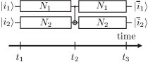
Figure 1: CNOT gate for two qubits subject to environmental noise. We assume that the two noises represented by the gates $N_{1}$ and $N_{2}$ are independent.

Such a quantum circuit is interesting because the final state of the target qubit will depend not only on the noise acting on it but, through the CNOT gate, also on the noise acting on the control qubit: the noise gate formalism allows this dependence to analyzed in simple terms. For definiteness, let us take $|0,0\rangle$ as the input state. Let us moreover assume that the noises acting on the two qubits are independent of each other; this assumption is of course justified only if, e.g., the two physical states encoding the two qubits are separated by more than the correlation length of the noise, so that the surrounding environment acts independently on them.

The noisy CNOT gate acts on the qubits as follows:

$$|0,0\rangle \xrightarrow[]{(1)} N_{1}(t_{2},t_{1})\otimes N_{2}(t_{2},t_{1})\ket{0,0}$$ (15)

$$= \sum_{i,j=0}^{1}n_{1}^{(i,0)}(t_{2},t_{1})n_{2}^{(j,0)}(t_{2},t_{1})|i,j\rangle$$

$$\xrightarrow[]{(2)} \sum_{i,j=0}^{1}n_{1}^{(i,0)}(t_{2},t_{1})n_{2}^{(j,0)}(t_{2},t_{1})|i,i\oplus j\rangle$$

$$\xrightarrow[]{(3)} \sum_{i,j=0}^{1}\sum_{m,\ell=0}^{1}n_{1}^{(i,0)}(t_{2},t_{1})n_{2}^{(j,0)}(t_{2},t_{1})$$

$$\cdot n_{1}^{(m,i)}(t_{3},t_{2})n_{2}^{(\ell,i\oplus j)}(t_{3},t_{2})|m,\ell\rangle,$$

where $n_{\alpha}^{(i,j)}(t_{b},t_{a})$ is the $(i,j)$-th coefficient of the matrix $N_{\alpha}(t_{b},t_{a})$, $\alpha=1,2$. Step (1) takes into account the effect of the environment from time $t_{1}$ to time $t_{2}$, after which the CNOT gate is applied: the latter corresponds to step (2). In step (3) we assume that the environment acts on the qubits until time $t_{3}$. Let us call $|\overline{0,0}\rangle$ the final state.

For a closed system we would have of course $|\overline{0,0}\rangle=|0,0\rangle$, but with the environment interacting with the two qubits, $|\overline{0,0}\rangle$ becomes a random entangled state; to understand the effect of the noise, let us compute the fidelity $F\equiv{\mathbb{E}}[|\langle 0,0|\overline{0,0}\rangle|^{2}]$ of the noisy protocol (the stochastic average ${\mathbb{E}}$ takes into account all possible realizations of the noise). Because of the Markov property of Wiener processes, we have the following property:

Property 1. Two gates $N(t_{2},t_{1})$ and $N(t_{4},t_{3})$ are independent whenever $(t_{1},t_{2})\cap(t_{3},t_{4})$ is empty. This follows directly from the fact that a Brownian motion has independent increments.

According to this rule, and keeping in mind the assumption that the noise gates acting on the two qubits are also independent, $F$ is a combination only of terms having the form ${\mathbb{E}}[n_{\alpha}^{(i,k)}(t_{b},t_{a})n_{\alpha}^{(i^{\prime},k^{\prime})}(t_{b},t_{a})^{\star}]$ with $\alpha=1,2$ and $(t_{b},t_{a})=(t_{2},t_{1})$ or $(t_{3},t_{2})$, since all other terms vanish when averaged, because of the statistical independence. Now it is just a matter of choosing the type of noise that best describes the environment, and computing the required expectation values.

Let us consider, as an example, the bit flip gate given in Eq. (6):

$$N_{\makebox{\tiny BitFl}}(t,t_{0})=\left(\begin{array}[]{cc}\cos(\sqrt{\gamma}\Delta W_{t})&i\sin(\sqrt{\gamma}\Delta W_{t})\\ i\sin(\sqrt{\gamma}\Delta W_{t})&\cos(\sqrt{\gamma}\Delta W_{t})\end{array}\right),$$ (16)

with $\Delta W_{t}=W_{t}-W_{t_{0}}$; one easily verifies that, for a standard Wiener process, the following equalities hold true:

$${\mathbb{E}}[\cos^{2}(\sqrt{\gamma_{\alpha}}(W_{t_{b}}-W_{t_{a}}))] = p_{\alpha}(t_{b}-t_{a})$$

$$\equiv \frac{1+\exp[-2\gamma_{\alpha}(t_{b}-t_{a})]}{2}$$

$${\mathbb{E}}[\sin^{2}(\sqrt{\gamma_{\alpha}}(W_{t_{b}}-W_{t_{a}}))] = \overline{p}_{\alpha}(t_{b}-t_{a})$$

$$\equiv 1-p_{\alpha}(t_{b}-t_{a}),$$

while ${\mathbb{E}}[\cos(\sqrt{\gamma_{\alpha}}(W_{t_{b}}-W_{t_{a}}))\sin(\sqrt{\gamma_{\alpha}}(W_{t_{b}}-W_{t_{a}}))]=0$. From these expressions one can derive the following expressions for the correlation functions of the coefficients of the noise gate:

$${\mathbb{E}}[n_{\alpha}^{(i,k)}(t_{b},t_{a})n_{\alpha}^{(i^{\prime},k^{\prime})}(t_{b},t_{a})^{\star}] = p_{\alpha}(t_{b}-t_{a})$$

$$\text{if $i=k$, $i^{\prime}=k^{\prime}$};$$

$${\mathbb{E}}[n_{\alpha}^{(i,k)}(t_{b},t_{a})n_{\alpha}^{(i^{\prime},k^{\prime})}(t_{b},t_{a})^{\star}] = \overline{p}_{\alpha}(t_{b}-t_{a})$$

$$\text{if $i\neq k$, $i^{\prime}\neq k^{\prime}$};$$

$${\mathbb{E}}[n_{\alpha}^{(i,k)}(t_{b},t_{a})n_{\alpha}^{(i^{\prime},k^{\prime})}(t_{b},t_{a})^{\star}] = 0$$

$$\text{in all other cases}.$$

Given this, one easily gets the following expression for the fidelity $F$ as a function of the coupling constants $\gamma_{\alpha}$ and of the time intervals during which the noises act on the CNOT gate:

$$F = p_{1}(t_{2}-t_{1})p_{2}(t_{2}-t_{1})p_{1}(t_{3}-t_{2})p_{2}(t_{3}-t_{2})$$ (22)

$$+ \overline{p}_{1}(t_{2}-t_{1})p_{2}(t_{2}-t_{1})\overline{p}_{1}(t_{3}-t_{2})\overline{p}_{2}(t_{3}-t_{2})$$

$$+ p_{1}(t_{2}-t_{1})\overline{p}_{2}(t_{2}-t_{1})p_{1}(t_{3}-t_{2})\overline{p}_{2}(t_{3}-t_{2})$$

$$+ \overline{p}_{1}(t_{2}-t_{1})\overline{p}_{2}(t_{2}-t_{1})\overline{p}_{1}(t_{3}-t_{2})p_{2}(t_{3}-t_{2}).\;\;\;\;\;\;$$

In particular, if we assume that the two noises have the same strength ($\gamma_{1}=\gamma_{2}$) and that the time intervals during which they act are the same $t_{3}-t_{2}=t_{2}-t_{1}=T$, we obtain the simplified formula:

$$F(T)=4p(t)^{3}-5p(T)^{2}+2p(T),\;\;p(T)=\frac{1+e^{-2\gamma T}}{2},$$ (23)

which shows, as expected, that $F$ starts from 1 and decreases exponentially in time to $1/4$: the formula displays the whole time evolution.

V Application 2: Transfer of an entangled state through a spin chain.

One of the most common problems in quantum information theory is the transfer of information through a noisy channel, which is often analyzed by modeling the channel with a spin chain sc . By means of the spin chain (see Fig. 2) we want to demonstrate the power of the noise gate formalism for analyzing whole quantum circuits.

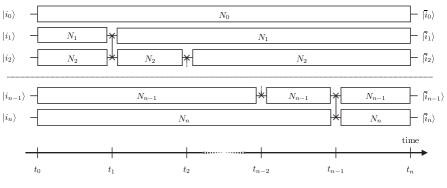
Figure 2: Quantum circuit for the transmission of an entangled state through a spin chain in a noisy environment.

For the spin chain we chose a standard model consisting of a chain of $n+1$ qubits, such that the first two qubits are in a given normalized entangled state $|\psi\rangle$, while the remaining qubits are in a general normalized state $|\phi\rangle$; then the global initial state is $|\Psi\rangle=|\psi\rangle\otimes|\phi\rangle$ with

$$|\psi\rangle = \sum_{i_{0},i_{1}=0}^{1}a_{i_{0},i_{1}}|i_{0}i_{1}\rangle$$ (24)

$$|\phi\rangle = \sum_{i_{2},\ldots i_{n}=0}^{1}c_{i_{2},\ldots i_{n}}|i_{2}\ldots i_{n}\rangle.$$ (25)

The state of qubit 1 can be transferred to the far end of the chain by means of a sequence of $n-2$ swap operations; for a circuit not subject to noise, at the end of the protocol the first and last qubits are in the entangled state $|\psi\rangle$, factorized from the rest of the chain: we now analyze how the protocol is changed by the effect of a noisy environment, which we describe by $n+1$ noise gates $N_{k}(t_{i},t_{j})$, $k=1,\ldots,n$, each acting on a different qubit for the time interval ($t_{j},t_{i}$). We assume that the environment is random enough to act independently on each qubit; this means that we assume that the noise gates are independent.

The time evolution of the global state can now be immediately computed: due to the linearity of the noise gates, and with reference to Fig. 2, one easily gets for the final state at time $t=t_{n}$

$$|\overline{\Psi}\rangle=\sum_{i_{0},\ldots i_{n}}a_{i_{0},i_{1}}\,c_{i_{2},\ldots i_{n}}\,|\bar{i}_{0}\rangle\otimes|\bar{i}_{1}\rangle\otimes\ldots|\bar{i}_{n}\rangle,$$ (26)

where the states $|\bar{i}_{k}\rangle$ are defined as follows:

$$|\bar{i}_{0}\rangle = N_{0}(t_{n},t_{0})\,|i_{0}\rangle,$$

$$|\bar{i}_{k}\rangle = N_{k}(t_{n},t_{k})N_{k+1}(t_{k},t_{0})\,|i_{k+1}\rangle,\;\;k=1,\ldots n-1$$

$$|\bar{i}_{n}\rangle = \prod_{k=0}^{n-1}N_{n-k}(t_{n-k},t_{n-k-1})\,|i_{1}\rangle;$$ (27)

so the problem is mathematically solved. In order to test the effect of the environment on the transmission protocol, we compute the reduced density matrix referring to the 0th and $n$th qubits, obtained from the full density matrix ${\mathbb{E}}[|\overline{\Psi}\rangle\langle\overline{\Psi}|]$ by tracing away all other degrees of freedom (from 1 to $n-1$):

$$\rho_{(0,n)}(t_{n}) = \text{Tr}_{1,\ldots,(n-1)}{\mathbb{E}}[|\overline{\Psi}\rangle\langle\overline{\Psi}|]$$ (28)

$$= {\mathbb{E}}[|\bar{\psi}\rangle\langle\bar{\psi}|\cdot\text{Tr}|\bar{\phi}\rangle\langle\bar{\phi}|],$$ (29)

where we have defined:

$$|\bar{\psi}\rangle = \sum_{i_{0},i_{1}=0}^{1}a_{i_{0},i_{1}}N_{0}(t_{n},t_{0})\,|i_{0}\rangle\overline{N}\,|i_{1}\rangle$$

$$|\bar{\phi}\rangle = \sum_{i_{2},\ldots i_{n}=0}^{1}c_{i_{2},\ldots i_{n}}\underline{N}_{1}\,|i_{2}\rangle\ldots\underline{N}_{n-1}\,|i_{n}\rangle,$$ (30)

and we have used the short-hand notation:

$$\underline{N}_{k} \equiv N_{k}(t_{n},t_{k})N_{k+1}(t_{k},t_{0})$$ (31)

$$\overline{N} \equiv \prod_{k=0}^{n-1}N_{n-k}(t_{n-k},t_{n-k-1}).$$ (32)

Note that the state $|\bar{\psi}\rangle$ is a linear combination of the two states $|\bar{i}_{0}\rangle$ and $|\bar{i}_{n}\rangle$ (see Fig. 2)—this is the reason why the trace does not affect $|\bar{\psi}\rangle\langle\bar{\psi}|$—while $|\bar{\phi}\rangle$ is a linear combination of the remaining states $|\bar{i}_{1}\rangle,\ldots|\bar{i}_{n-1}\rangle$.

In our setting, Property 1 together with our assumption of independence of the environments lead to the independence of the statistics of the noise gates $N_{i}(t_{v},t_{u})$ and $N_{j}(t_{s},t_{r})$ whenever $i\neq j$ or $(t_{u},t_{v})\cap(t_{r},t_{s})$ is empty. One easily verifies that $N_{0}(t_{n},t_{0})$, $\overline{N}$ and $\underline{N}_{k}$ for $k=1,\ldots,n-1$ are independent; this can be immediately checked in Fig. 2. This also means that the statistics of $|\bar{\psi}\rangle\langle\bar{\psi}|$ is independent of that of $|\bar{\phi}\rangle\langle\bar{\phi}|$, and their average values can be computed separately:

$$\rho_{(0,n)}(t_{n}) = {\mathbb{E}}[|\bar{\psi}\rangle\langle\bar{\psi}|]\cdot{\mathbb{E}}[\text{Tr}|\bar{\phi}\rangle\langle\bar{\phi}|].$$ (33)

Another important property of the noise gates, which we shall now use to simplify the above formula, is the following.

Property 2. Given an initial normalized $n$-qubit state $|\psi_{0}\rangle$ which evolves, according to a SDE of the type (2), to a random state $|\psi_{t}\rangle=N(t,t_{0})|\psi_{0}\rangle$, then the following equality holds true: $\text{Tr}\,{\mathbb{E}}[|\psi_{t}\rangle\langle\psi_{t}|]=1$ for any $t$. This property is a direct consequence of Eq. (3) and of the fact that $\rho(t)$ satisfies Eq (1), which is of the Lindblad type and thus trace preserving.

For the sake of brevity, we denote $i_{2},\ldots,i_{n}$ by $\underline{i}$; the full expression of $\text{Tr}\mathbb{E}[|\ket{\bar{\phi}}\bra{\bar{\phi}}]$ is, according to Eq. (30),

$$\text{Tr}\mathbb{E}[|\ket{\bar{\phi}}\bra{\bar{\phi}}]=\sum_{\underline{j}}\mathbb{E}\Big{[}\sum_{\underline{i},\underline{i}^{\prime}}c_{\underline{i}}c^{*}_{\underline{i}^{\prime}}\prod_{k=2}^{n}\braket{j_{k}}{N_{k-1}(t_{n},t_{k-1})N_{k}(t_{k-1},t_{0})}{i_{k}}\braket{i^{\prime}_{k}}{N^{*}_{k}(t_{k-1},t_{0})N^{*}_{k-1}(t_{n},t_{k-1})}{j_{k}}\Big{]};$$ (34)

we now insert two identities $\sum_{\underline{l}}\ket{\underline{l}}\bra{\underline{l}}$ between the noise matrices, and after a rearrangement of the terms we get

$$\text{Tr}\mathbb{E}[|\ket{\bar{\phi}}\bra{\bar{\phi}}]=\sum_{\underline{i},\underline{i}^{\prime},\underline{l},\underline{l}^{\prime}}\prod_{k=2}^{n}\underbrace{\text{Tr}\mathbb{E}\Big{[}N_{k-1}(t_{n},t_{k-1})\ket{l_{k}}\bra{l^{\prime}_{k}}N^{*}_{k-1}(t_{n},t_{k-1})\Big{]}}_{(\Delta)}\cdot\mathbb{E}\Big{[}c_{\underline{i}}c^{*}_{\underline{i}^{\prime}}\braket{l_{k}}{N_{k}(t_{k-1},t_{0})}{i_{k}}\braket{i^{\prime}_{k}}{N^{*}_{k}(t_{k-1},t_{0})}{l^{\prime}_{k}}\Big{]},$$ (35)

where the factorization of the two average values is again justified by the assumption of independence of the environments and by Property 1.

By Property 2, we have

$$(\Delta)\;=\;\text{Tr}\mathbb{E}\Big{[}\ket{l_{k}}\bra{l^{\prime}_{k}}\Big{]}\;=\;\delta_{l_{k},l^{\prime}_{k}},$$ (36)

so Eq. (35) simplifies as follows:

$$\text{Tr}\mathbb{E}[|\ket{\bar{\phi}}\bra{\bar{\phi}}]=$$

$$= \text{Tr}\mathbb{E}\Big{[}\sum_{\underline{i},\underline{i}^{\prime}}\prod_{k=2}^{n}c_{\underline{i}}c^{*}_{\underline{i}^{\prime}}N_{k}(t_{k-1},t_{0})\ket{i_{k}}\bra{i^{\prime}_{k}}N^{*}_{k}(t_{k-1},t_{0})\Big{]},$$

which, again by Property 2, gives

$$\text{Tr}\mathbb{E}[|\ket{\bar{\phi}}\bra{\bar{\phi}}]=\text{Tr}\ket{\phi}\bra{\phi}=1.$$ (38)

Accordingly we are left with the expected simple result:

$$\rho_{(0,n)}(t_{n})\;=\;{\mathbb{E}}[|\bar{\psi}\rangle\langle\bar{\psi}|],$$ (39)

from which any relevant piece of information can be obtained.

V.1 Fidelity of the transmission protocol

As an application of this formula we now compute the fidelity

$$F=\text{Tr}[\rho_{(0,n)}(t_{n})|\psi\rangle\langle\psi|]={\mathbb{E}}[|\langle\psi|\bar{\psi}\rangle|^{2}]$$ (40)

of the transmission protocol; here, again, the noise gates come in handy in the computation since we may work with random vectors instead of density matrices. In order to focus our attention only on the effect of the noise on the qubit that has been transmitted, we neglect the effect of the noise gate $N_{0}(t_{n},t_{0})$ on the 0th qubit. We denote the random matrix components of $\bar{N}$ by

$$\bar{N}=\begin{pmatrix}\bar{a}&\bar{b}\\ \bar{c}&\bar{d}\end{pmatrix}$$ (41)

and compute

$$\braket{\psi}{\bar{\psi}} =\sum_{i_{0},i_{1},j_{0},j_{1}}a^{*}_{j_{0},j_{1}}a_{i_{0},i_{1}}\bra{j_{0}j_{1}}\mathbbm{1}\otimes\bar{N}\ket{i_{0}i_{1}}$$ (42)

$$=A\bar{a}+B\bar{b}+B^{*}\bar{c}+(1-A)\bar{d},$$ (43)

where

$$A:=|a^{\phantom{\star}}_{0,0}|^{2}+|a^{\phantom{\star}}_{1,0}|^{2}, B:=a^{\star}_{0,0}a^{\phantom{\star}}_{0,1}+a^{\star}_{1,0}a^{\phantom{\star}}_{1,1}.$$ (44)

In order to become more concrete we chose the amplitude damping gate for $N_{k}$, cf. Eq. (14),

$$N_{k}(t_{k},t_{k-1}) =\begin{pmatrix}a_{k}&b_{k}\\ c_{k}&d_{k}\end{pmatrix}$$ (45)

$$:=\begin{pmatrix}1&i\sqrt{\gamma_{k}}\int_{t_{k-1}}^{t_{k}}e^{-\frac{\gamma_{k}}{2}s}dW^{(k)}_{s}\\ 0&e^{-\frac{\gamma_{k}}{2}(t_{k}-t_{k-1})}\end{pmatrix}.$$ (46)

The coupling constant $\gamma_{k}$ represents the strength of the interaction of the $k$-th noise $W^{(k)}$ with the $k$-th qubit. By definition of $\bar{N}$, cf. Eq. (32), its matrix components are given by

$$\bar{a}=1,\qquad\bar{c}=0,\qquad\bar{d}=\prod_{k=1}^{n}d_{k},$$ (47)

while $\bar{b}=\bar{b}_{n}$ (for $n$ qubits) is defined by the recursive formula $\bar{b}_{n}:=b_{n}+d_{n}\bar{b}_{n-1}$, with $\bar{b}_{1}=b_{1}$ where $\bar{b}_{1}=b_{1}$. Now we have all we need to compute the fidelity of this protocol. Plugging these matrix components into Eq. (43) we get by Eq. (39)

$$F =\mathbb{E}\left[|A\bar{a}+B\bar{b}+(1-A)\bar{d}|^{2}\right]$$ (48)

$$=A^{2}+|B|^{2}\mathbb{E}\left[|\bar{b}|^{2}\right]+(1-A)^{2}\bar{d}^{2}.$$ (49)

In the last step we have used the fact that only $\bar{b}$ is random and that only the terms quadratic in $\bar{b}$ give a non zero contribution to the expectation value. Using the recursive definition of $\bar{b}$, cf. Eq. (47), and again collecting only the terms quadratic in the random variables $b_{k}$, we compute

$$\mathbb{E}\left[|\bar{b}|^{2}\right] =\mathbb{E}\left[|\bar{b}_{n}+d_{n}\bar{b}_{n-1}|^{2}\right]$$ (50)

$$=\mathbb{E}\left[|\bar{b}_{n}|^{2}]+d_{n}^{2}\mathbb{E}[|\bar{b}_{n-1}|^{2}\right]$$ (51)

$$=1-e^{-\Gamma},\quad\Gamma=\sum_{\alpha=1}^{n}\gamma_{\alpha}(t_{\alpha}-t_{\alpha-1})$$ (52)

by induction. Together with $\bar{d}=e^{-\frac{\Gamma}{2}}$ we arrive at the formula:

$$F_{\makebox{\tiny AmDa}}=\left[A+(1-A)e^{-\frac{\Gamma}{2}}\right]^{2}+|B|^{2}(1-e^{-\Gamma})$$ (53)

For the bit flip, the phase flip and the bit-phase flip channels, cf. (6)-(8), we use the noise gates

$$N_{l}(t_{l},t_{l-1})=\exp\left(i\sqrt{\gamma_{l}}\sigma_{\kappa}(W_{t_{l}}-W_{t_{l-1}})\right)$$ (54)

with $\kappa=x,z,y$, respectively, and so compute $\bar{N}$ for the three cases according to equation (32):

$$\bar{N}_{\makebox{\tiny BitFl}}=\begin{pmatrix}\cos\phi&&i\sin\phi\\ i\sin\phi&&\cos\phi\end{pmatrix},$$ (55)

$$\bar{N}_{\makebox{\tiny PhFl}}=\begin{pmatrix}e^{i\phi}&&0\\ 0&&e^{-i\phi}\end{pmatrix},$$ (56)

$$\bar{N}_{\makebox{\tiny BitPhFl}}=\begin{pmatrix}\cos\phi&&\sin\phi\\ -\sin\phi&&\cos\phi\end{pmatrix}$$ (57)

for

$$\phi=\sum_{k=0}^{n-1}\sqrt{\gamma_{k}}\left(W_{t_{n-k}}-W_{t_{n-k-1}}\right).$$ (58)

Using equation (42) the fidelity turns out to be

$$F_{\makebox{\tiny BitFl}} =\mathbb{E}\left(\cos^{2}\phi+4\text{Re}B^{2}\sin^{2}\phi\right)$$ (59)

$$F_{\makebox{\tiny PhFl}} =\mathbb{E}\left(|1+A(e^{2i\phi}-1)|^{2}\right)$$ (60)

$$F_{\makebox{\tiny BitPhFl}} =\mathbb{E}\left(\cos^{2}\phi+4\text{Im}B^{2}\sin^{2}\phi\right),$$ (61)

Here Re and Im denote the real and imaginary parts respectively. After evaluation of the expectation value the fidelity is given by

$$F_{\kappa}=\frac{1+g_{\kappa}^{2}}{2}+\frac{1-g_{\kappa}^{2}}{2}e^{-2\Gamma},$$ (62)

where $\kappa$ denotes BitFl, PhFl BitPhFl, and $g_{\makebox{\tiny BitFl}}=2\text{Re}\,B$, $g_{\makebox{\tiny PhFl}}=2A-1$ and $g_{\makebox{\tiny Bit-PhFl}}=2\text{Im}\,B$. As expected, the fidelity decreases exponentially in time, reaching an asymptotic finite value which depends both on the initial entangled state and on the type of noise. More generally, the above formula displays the full dependence of $F$ on the different parameters entering the protocol, in particular on the time between two subsequent application of a swap operation and on the strength of the different noises. It then applies, e.g. to non homogeneous environments, where some qubits feel a stronger decoherence effect than others. One can easily generalize the above result by including also uncertainties in the times at which the different swap operations are applied.

VI Linear Combinations of Noises

So far we have looked only at SDEs that are explicitly solvable. In this section we want to consider more complicated noise channels for which an explicit solution might not be available. In the chosen examples of this section we shall see that this is already the case when we combine two or more of the noise channels that we have discussed so far.

In general, a linear combination of noises acting on the same quantum system can be described by

$$d|\psi_{t}\rangle=\sum_{\kappa}\left[i\sqrt{\gamma^{(\kappa)}}\,L_{\kappa}\,dW_{t}^{(\kappa)}-\frac{1}{2}\,\gamma^{(\kappa)}L_{\kappa}^{\dagger}L_{\kappa}dt\right]|\psi_{t}\rangle,$$ (63)

where in contrast to (2) we have neglected the Hamiltonian but in addition have multiple Brownian motions $W_{t}^{(\kappa)}$. For Lindblad operators $L_{\kappa}$ this in turn leads to the corresponding master equation

$$\frac{d}{dt}\,\rho(t)=\sum_{\kappa}\left[\gamma^{(\kappa)}L_{\kappa}\rho(t)L^{\dagger}_{\kappa}-\frac{\gamma^{(\kappa)}}{2}\,\{L^{\dagger}_{\kappa}L_{\kappa},\rho(t)\}\right]$$ (64)

in the sense that (3) holds accordingly.

As an important feature of the noise gate formalism we notice that, since quantum averages are always expressed as the square modulus of the scalar product of two vectors, the coefficients of the noise gates always enter the stochastic averages in quadratic combinations, which with a little abuse of terminology we shall refer to as second moments. Now, although (63) might not in general be explicitly solvable it is often possible to infer from it all second moments of the noise gate that it describes either analytically or numerically; see arn for a discussion of this topic. As we shall demonstrate, this can be done in an easy way whenever a solution to the corresponding master equation is available. Having these second moments computed either analytically or numerically, one may still work in the noise gate picture even without having the explicit form of the noise gate, which in many circumstances can be more intuitive and faster. For the following discussion let us denote the $(i,j)$-th unknown coefficient of a noise gate $N(t_{b},t_{a})$ by $n^{(ij)}(t_{b},t_{a})$, $i,j=0,1$. Then, if the second moments of this noise gate, i.e. $\mathbb{E}\left(n^{(ij)}(t_{b},t_{a}){n^{(kl)}(t_{b},t_{a})}^{*}\right)$ for any $i,j,k,l=0,1$, are available one may perform any computation of a quantum average using the noise gate formalism and in the end plug in the second moments when evaluating the stochastic average.

In order to compute the second moments whenever a solution of the master equation is available, consider $\ket{\psi(t_{a})}$ to be the initial value of the SDE and $\rho(t_{a})=\ket{\psi(t_{a})}\bra{\psi(t_{a})}$ the initial value of the master equation, both at time $t_{a}$. As discussed before, the solution to the SDE at time $t_{b}$ can be expressed via the noise gate it describes as $N(t_{b},t_{a})\ket{\psi(t_{a})}$. By (3) the two entities $\rho(t_{b})$ and $\mathbb{E}(N(t_{b},t_{a})\ket{\psi(t_{a})}\bra{\psi(t_{a})}N(t_{b},t_{a})^{*})$ must be equal. For $\ket{\psi(t_{a})}=\sum_{i}a_{i}\ket{i}$ we have

$$\rho_{00}(t_{b}) =|a_{0}|^{2}\mathbb{E}\left(|n^{(00)}_{T}|^{2}\right)+|a_{1}|^{2}\mathbb{E}\left(|n^{(01)}_{T}|^{2}\right)+2\text{Re}a_{0}a_{1}^{*}\mathbb{E}\left(n^{(00)}_{T}{n^{(01)}_{T}}^{*}\right)$$ (65)

$$\rho_{01}(t_{b}) =|a_{0}|^{2}\mathbb{E}\left(n^{(00)}_{T}{n^{(10)}_{T}}^{*}\right)+|a_{1}|^{2}\mathbb{E}\left(n^{(01)}_{T}{n^{(11)}_{T}}^{*}\right)+a_{0}a_{1}^{*}\mathbb{E}\left(n^{(00)}_{T}{n^{(11)}_{T}}^{*}\right)+a_{0}^{*}a_{1}\mathbb{E}\left(n^{(01)}_{T}{n^{(10)}_{T}}^{*}\right)=\rho_{10}(t_{b})^{*}$$ (66)

$$\rho_{11}(t_{b}) =|a_{0}|^{2}\mathbb{E}\left(|n^{(10)}_{T}|^{2}\right)+|a_{1}|^{2}\mathbb{E}\left(|n^{(11)}_{T}|^{2}\right)+2\text{Re}a_{0}a_{1}^{*}\mathbb{E}\left(n^{(10)}_{T}{n^{(11)}_{T}}^{*}\right),$$ (67)

where $\rho_{ij}(t)=\braket{i}{\rho(t)}{j}$ and $T=t_{b}-t_{a}$. Coefficient comparison then easily leads to the second moments.

In the following we apply this scheme to the spin chain of the previous section treating two prominent representatives of combined noise channels which are known as depolarizing and generalized amplitude damping channel, see nc .

VI.1 Depolarizing Channel

The depolarizing channel is a linear combination of the bit flip, phase flip and bit-phase flip channels. In terms of Eq. (63), $\kappa=1,2,3$ and the $L_{\kappa}$ are the Pauli matrices $\sigma_{x},\sigma_{y},\sigma_{z}$. Here the effect of the environment is to randomly rotate the qubit around the $x,y,z$ axis, with the randomization being proportional to the strength of the coupling constants $\gamma^{(1)},\gamma^{(2)},\gamma^{(3)}$.

Hence its master equation takes the following form:

$$\frac{d}{dt}\rho(t)=\begin{pmatrix}(\rho_{11}(t)-\rho_{00}(t))\gamma^{(1,2)}&&\rho_{10}(t)(\gamma^{(1)}-\gamma^{(2)})-\rho_{01}(t)(\gamma^{(1)}+\gamma^{(2)}+2\gamma^{(3)})\\ \rho_{01}(t)(\gamma^{(1)}-\gamma^{(2)})-\rho_{10}(t)(\gamma^{(1)}+\gamma^{(2)}+2\gamma^{(3)})&&(\rho_{00}(t)-\rho_{11}(t))\gamma^{(1,2)}\end{pmatrix},$$ (68)

for which

$$\rho_{00}(t_{b}) =\frac{1}{2}\left(|a_{0}|^{2}(1+e^{-2T\gamma^{(1,2)}})+|a_{1}|^{2}(1-e^{-2T\gamma^{(1,2)}})\right)$$ (69)

$$\rho_{01}(t_{b}) =\frac{1}{2}\left(a_{0}a_{1}^{*}(e^{-2T\gamma^{(1,3)}}+e^{-2T\gamma^{(2,3)}})+a_{0}^{*}a_{1}(e^{-2T\gamma^{(2,3)}}-e^{-2T\gamma^{(1,3)}})\right)=\rho_{10}(t_{b})^{*}$$ (70)

$$\rho_{11}(t_{b}) =\frac{1}{2}\left(|a_{0}|^{2}(1-e^{-2T\gamma^{(1,2)}})+|a_{1}|^{2}(1+e^{-2T\gamma^{(1,2)}})\right)$$ (71)

is the solution for initial value $\rho(t_{a})$, where we have used $T=t_{b}-t_{a}$ and $\gamma^{(m,n)}=\gamma^{(m)}+\gamma^{(n)}$. By coefficient comparison with Eqs. (65), (66) and (67) one finds

$$\mathbb{E}(n^{(ij)}(t_{b},t_{a})n^{(i^{\prime}j^{\prime})}(t_{b},t_{a})^{\star})=$$

$$=\left\{\begin{array}[]{ll}\frac{1}{2}(1+e^{-2T\gamma^{(1,2)}})&,i=k=i^{\prime}=k^{\prime}\\ \frac{1}{2}(1-e^{-2T\gamma^{(1,2)}})&,i=k\neq i^{\prime}=k^{\prime}\\ \frac{1}{2}(e^{-2T\gamma^{(2,3)}}+e^{-2T\gamma^{(1,3)}})&,i,k,i^{\prime},k^{\prime}=0,0,1,1\\ \frac{1}{2}(e^{-2T\gamma^{(2,3)}}-e^{-2T\gamma^{(1,3)}})&,i,k,i^{\prime},k^{\prime}=0,1,1,0\\ 0&,\text{else}\end{array}\right.$$ (77)

In order to apply this noise channel to the spin chain circuit discussed above we only need to plug these terms into Eq. (40) where we use the same abbreviations as in Eq. (42). We shall label the coupling coefficients for the $\alpha$-th qubit by $\gamma_{\alpha}^{(1)},\gamma_{\alpha}^{(2)},\gamma_{\alpha}^{(3)}$ for all $\alpha=1,\ldots,n$ when evaluating the product in (32). The computation of the fidelity is then straight forward:

$$F_{\makebox{\tiny DePo}}=\frac{1}{2}(A^{2}+(1-A)^{2})(1+e^{-2\Gamma^{(1,2)}})+$$

$$+A(1-A)(e^{-2\Gamma^{(2,3)}}+e^{-2\Gamma^{(1,3)}})+$$

$$+|B|^{2}(1-e^{-2\Gamma^{(1,2))}})+\text{Re}B^{2}(e^{-2\Gamma^{(2,3))}}-e^{-2\Gamma^{(1,3))}})$$ (78)

where $\Gamma^{(m,n)}=\sum_{\alpha=1}^{N}(\gamma^{(m)}_{\alpha}+\gamma^{(n)}_{\alpha})(t_{\alpha}-t_{\alpha-1})$ and $\gamma^{(i)}_{\alpha}$ denotes the $i$th coupling constant of the $\alpha$th noise gate in the circuit. Note that the formula reduces to $F_{\kappa}$, Eq. (62), when all the coupling constants are set to zero except the ones associated with one Pauli matrix. Figure 3 displays the time evolution of the fidelity of the spin chain under the influence of the depolarizing channel for a specific class of initial states.

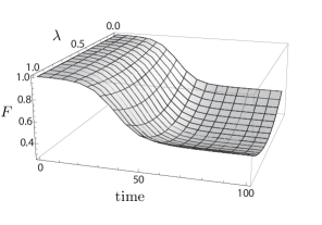
Figure 3: Time dependence of the fidelity $F$ of the qubit pair $\sqrt{\lambda}\ket{01}+\sqrt{1-\lambda}\ket{10}$ separated by the described spin chain circuit (see figure (2)) consisting of $100$ qubits under the influence of depolarizing channels, see Eq. (VI.1). The time intervals between the swap operations were chosen to be equal to $1$ while the coupling coefficients $\gamma^{(i)}_{\alpha}$ were chosen according to a Gaussian distribution centered around the $50$-th qubit with covariance $\operatorname{cov}_{i}$ such that $\operatorname{cov}_{1}:\operatorname{cov}_{2}:\operatorname{cov}_{3}=1:2:3$. Due to the chosen class of initial states, the curvature of the surface along the time axis is due to the coupling of $\gamma^{(1)}_{\alpha}$ and $\gamma^{(2)}_{\alpha}$ while $\gamma^{(3)}_{\alpha}$ determines the curvature along the $\lambda$ axis.

VI.2 Generalized Amplitude Damping Channel

The generalized amplitude damping channel in turn is a linear combination of the amplitude damping channel as defined in the previous sections and the inverse process for which $|1\rangle$ is stable and $|0\rangle$ decays. In terms of Eq. (63), $\kappa=1,2$ and the $L_{\kappa}$ are the operators $\sigma_{-}$ and $\sigma_{+}=|1\rangle\langle 0|$. The amplitude damping channel that we have discussed in the previous sections is the zero temperature limit of this channel. For non zero temperature the qubit may now also gain energy at the rate $\gamma^{(2)}$.

This time its master equation takes the following form:

$$\frac{d}{dt}\rho(t)=\begin{pmatrix}\rho_{11}(t)\gamma^{(1)}-\rho_{00}(t)\gamma^{(2)}&&-\frac{\rho_{01}(t)}{2}(\gamma^{(1)}+\gamma^{(2)})\\ -\frac{\rho_{10}(t)}{2}(\gamma^{(1)}+\gamma^{(2)})&&\rho_{00}(t)\gamma^{(2)}-\rho_{11}(t)\gamma^{(1)}\end{pmatrix},$$ (79)

for which

$$\rho(t_{b})=\begin{pmatrix}|a_{0}|^{2}\cdot\frac{\gamma^{(1)}+\gamma^{(2)}e^{-\Gamma T}}{\Gamma}+|a_{1}|^{2}\cdot\frac{\gamma^{(1)}(1-e^{-\Gamma T})}{\Gamma}&&a_{0}a_{1}^{*}e^{-\frac{\Gamma}{2}T}\\ a_{0}^{*}a_{1}e^{-\frac{\Gamma}{2}T}&&|a_{0}|^{2}\cdot\frac{\gamma^{(2)}(1-e^{-\Gamma T})}{\Gamma}+|a_{1}|^{2}\cdot\frac{\gamma^{(2)}+\gamma^{(1)}e^{-\Gamma T}}{\Gamma}\end{pmatrix}$$ (80)

is the solution for initial value $\rho(t_{a})$, where we used $T=t_{b}-t_{a}$ and $\Gamma=\gamma^{(1)}+\gamma^{(2)}$. Again, by coefficient comparison with Eq. (65), (66) and (67) one finds

$$\mathbb{E}(|n^{(00)}(t_{b},t_{a})|^{2}) =\frac{\gamma^{(1)}+\gamma^{(2)}e^{-\Gamma T}}{\Gamma}$$ (81)

$$\mathbb{E}(|n^{(01)}(t_{b},t_{a})|^{2}) =\frac{\gamma^{(1)}}{\Gamma}e^{-\Gamma T}$$ (82)

$$\mathbb{E}(|n^{(10)}(t_{b},t_{a})|^{2}) =\frac{\gamma^{(2)}}{\Gamma}e^{-\Gamma T}$$ (83)

$$\mathbb{E}(|n^{(11)}(t_{b},t_{a})|^{2}) =\frac{\gamma^{(2)}+\gamma^{(1)}e^{-\Gamma T}}{\Gamma}$$ (84)

and

$$\mathbb{E}(n^{(00)}(t_{b},t_{a}){n^{(11)}(t_{b},t_{a})}^{*}) =e^{-\frac{\Gamma}{2}T}$$ (85)

while all other second moments are equal to zero. As we have done with the depolarizing channel we apply this noise to the spin chain circuit discussed above and therefore we, again, only need to plug these terms into Eq. (40) using the same abbreviations as in Eq. (42). In order to keep the displayed formulas short we choose the coupling constants to be the same for all qubits, i.e. $\gamma^{(1)}_{\alpha}=\gamma^{(1)}$ and $\gamma^{(2)}_{\alpha}=\gamma^{(2)}$ for all $\alpha=1,\ldots,n$, when computing the product in (32). We then find

$$F_{\makebox{\tiny GeAmDa}}=(A^{2}\frac{\gamma^{(1)}}{\Gamma}+(1-A)^{2}\frac{\gamma^{(2)}}{\Gamma}+|B|^{2})+$$

$$+(A^{2}\frac{\gamma^{(2)}}{\Gamma}+(1-A)^{2}\frac{\gamma^{(1)}}{\Gamma}-|B|^{2})e^{-\Gamma(t_{n}-t_{0})}+$$

$$+2A(1-A)e^{-\frac{\Gamma}{2}(t_{n}-t_{0})}$$ (86)

for $\Gamma=\gamma^{(1)}+\gamma^{(2)}$ and $\gamma^{(i)}=\gamma^{(i)}_{\alpha}$, such that all noise gates $N_{\alpha}$ in the circuit have the same coupling constants. Note that also this formula reduces to (53) if $\gamma^{(2)}$ is set to zero. An example of the time evolution of the fidelity for a specific class of initial conditions under the influence of generalized amplitude damping is shown in figure 4.

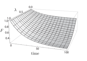
Figure 4: Time dependence of the fidelity $F$ of the qubit pair $\sqrt{\lambda}\ket{01}+\sqrt{1-\lambda}\ket{10}$ separated by the described spin chain circuit (see figure (2)) consisting of $100$ qubits under the influence of generalized amplitude damping channels, see Eq. (VI.2). The time intervals between the swap operations were chosen to be equal $1$ while $\gamma^{(1)}:\gamma^{(2)}:(\gamma^{(1)}+\gamma^{(2)})=3:1:4$. The latter is reflected in the curvature along the $\lambda$ axis.

VII Conclusion

We have suggested the noise gate formalism as a handy approach for analyzing the effect of the environment on quantum algorithms; it is very intuitive as it allows the influence of the environment to be treated in terms of noise gates, which can be manipulated like any other quantum gate. In many situations it makes the computation easier, either analytically or numerically. We emphasize again that it is especially interesting for numerical simulations because linear SDEs can be integrated by standard methods klo . In contrast to solving the Lindblad equation numerically, which roughly scales quadratically with the number of degrees of freedom, the numerical integration of (2) scales only linearly, even if the noises are dependent. Finally note that SDEs can also be generalized to model non Markovian quantum noise.

Acknowledgements. The work of A.B. has been partly supported by DFG (Germany). The work of D.-A.D. has been supported by the EU Grant No. ERG 044941-STOCH-EQ.

References

• (1) H-P. Breuer and F. Petruccione: The Theory of Open Quantum Systems, Oxford University Press, Oxford (2002).
• (2) M. A. Nielsen and I. L. Chuang: Quantum Computation and Quantum Information, Cambridge University Press, Cambridge U.K. (2000).
• (3) H. J. Carmichael: An Open Systems Approach to Quantum Optics (Springer, Berlin, 1993). M. Plenio and P. Knight, Rev. Mod. Phys. 70, 101 (1998). G. G. Carlo, G. Benenti and G. Casati Phys. Rev. Lett. 91, 257903 (2003). A. Carollo, I. Fuentes-Guridi, M. Franca Santos and V. Vedral, Phys. Rev. Lett. 90, 160402 (2003); 92, 020402 (2004).
• (4) N. Gisin and I. C. Percival, J. Phys. A: Math. Gen. 25, 5677 (1992); 26, 2233 (1993); 26, 2245 (1993). N. Gisin and M. Rigo, J. Phys. A: Math. Gen. 28, 7375 (1995). J. Halliwell, A. Zoupas, Phys. Rev. D 52, 7294 (1995); 55, 4697 (1997). T.A. Brun, N. Gisin, P.F. O’Mahony, M. Rigo, Phys. Lett. A 229, 267 (1997). I. Percival: Quantum State Diffusion, Cambridge University Press, Cambridge U.K. (1998). T. A. Brun, Am. J. Phys. 70, 719 (2002).
• (5) K. Jacobs and P. L. Knight, Phys. Rev. A 57, 2301 (1998). A. Bassi, Phys. Rev. A 67, 062101 (2003).
• (6) W. T. Strunz, L. Diosi, N. Gisin and T. Yu, Phys. Rev. Lett. 83, 4909 (1999). W. T. Strunz and L. Diosi, N. Gisin Phys. Rev. Lett. 82, 1801 (1999). A. A. Budini, Phys. Rev. A 63, 012106 (2000). J. Gambetta and H. M. Wiseman, J. Opt. B: Quantum Semiclass. Opt. 6, S821 (2004).
• (7) H.-P. Breuer, J. Gemmer and M. Michel, Phys. Rev. E 73, 016139 (2006). S. Maniscalco and F. Petruccione, Phys. Rev. A 73,012111 (2006). H.-P. Breuer, Phys. Rev. A 75, 022103 (2007). C. Lazarou, G. M. Nikolopoulos, P. Lambropoulos, preprint arXiv:0705.1616, to appear in J. Phys. B.
• (8) B.L. Hu, J.P. Paz and Y. Zhang, Phys. Rev. D 45, 2843 (1992). P. $\check{\text{S}}$telmachovi$\check{\text{c}}$ and V. Bu$\check{\text{z}}$ek, Phys. Rev. A 64, 062106 (2001). J. Schliemann, A. Khaetskii, and D. Loss, J. Phys.: Condens. Matter 15, R1809 (2003). J. Gemmer and M. Michel, Europhys. Lett. 73, 1 (2006).
• (9) P. E. Kloeden, E. Platen: Numerical Solutions of Stochastic Differential Eqautions, Springer Verlag, Berlin (1992).
• (10) D. Gatarek and N. Gisin, J. Math. Phys. 32, 2152 (1991). A.S. Holevo, Probab. Theor. Relat. Fields 104, 483 (1996). A. Bassi, Journ. Phys. A: Math. Gen. 38, 3173 (2005).
• (11) G.G. Carlo, G. Benenti, G. Casati, Phys. Rev. Lett. 91, 257903 (2003). G.G. Carlo, G. Benenti, G. Casati, C. Mejia-Monasterio, Phys. Rev. A 69, 062317 (2004). J.A. Hoyos, G. Rigolin, Phys. Rev. A 74, 062324 (2006). M. B. Plenio, S. Virmani, Phys. Rev. Lett. 99, 120504 (2007). K. Eckert, O. Romero-Isart, A. Sanpera, New J. Phys. 9, 155 (2007). J. Gong, P. Brumer, Phys. Rev. A 75, 032331 (2007).
• (12) L. Arnold: Stochastic Differential Equations: Theory and Applications, John Wiley (1974).