Quantum field theory in terms of consistency conditions I:
General framework, and perturbation theory via Hochschild cohomology

Abstract

In this paper, we propose a new framework for quantum field theory in terms of consistency conditions. The consistency conditions that we consider are “associativity” or “factorization” conditions on the operator product expansion (OPE) of the theory, and are proposed to be the defining property of any quantum field theory. Our framework is presented in the Euclidean setting, and is applicable in principle to any quantum field theory, including non-conformal ones. In our framework, we obtain a characterization of perturbations of a given quantum field theory in terms of a certain cohomology ring of Hochschild-type. We illustrate our framework by the free field, but our constructions are general and apply also to interacting quantum field theories. For such theories, we propose a new scheme to construct the OPE which is based on the use of non-linear quantized field equations.

1 Introduction

Quantum field theory has been formulated in different ways, the most popular ones being the path-integral approach and the operator formalism. In the path integral approach, one aims to construct the correlation functions of the theory as the moments of some measure on the space of classical field configurations. In the operator formalism, the quantum fields are viewed as linear operators which can act on physical states.

The path integral has the advantage of being closely related to classical field theory. In fact, the path integral measure is, at least formally, directly given in terms of the classical action of the theory. The operator formalism is more useful in contexts where no corresponding classical theory—and hence no Lagrange formalism—is known for the quantum field theory. It has been used extensively in the context of conformal or integrable field theories in two spacetime dimensions. In the operator formalism, one may take the point of view that the theory is determined by the algebraic relations between the quantum field observables. This viewpoint was originally proposed in a very abstract form by Haag and Kastler, see e.g. [1]. Other proposals aimed in particular at conformal field theories include e.g. the approach via vertex operator algebras due to Borcherds, Frenkel, Lopowski, Meurman and others [2, 3, 4, 5], see also a related proposal by Gaberdiel and Goddard [6]. A different approach of an essentially algebraic nature applicable to ”globally conformally invariant quantum field theories” in $D$ dimensions is due to [7, 8]. Approaches emphasizing the algebraic relations between the fields have also turned out to fundamental to the construction of quantum field theories on general curved backgrounds [9, 10, 11, 12], because in this case there is no preferred Hilbert space representation or vacuum state.

One way to encode the algebraic relations between the fields in a very explicit way (at least at short distances) is the Wilson operator product expansion (OPE) [13, 14, 15]. This expansion is at the basis of the modern treatments of two-dimensional conformal field theory, and it is a key tool in the quantitative analysis of asymptotically free quantum gauge theories in four dimensions such as Quantum Chromo Dynamics. The OPE can also be established for perturbative quantum field theory in general curved spacetimes [16]. In this reference, it was observed in particular that the OPE coefficients satisfy certain ”asymptotic clustering” or ”factorization” relations when various groups of points in the operator products are scaled together at different rates. This observation was taken one step further in [17], where it was suggested that the OPE should in fact be viewed as the fundamental datum describing a quantum field theory on curved (and flat) spacetimes, and that the factorization conditions should be viewed as the essential constraints upon the OPE coefficients.

In this paper, we will analyze these constraints on the OPE coefficients, and thereby formulate a new approach to quantum field theory in terms of the resulting consistency conditions. One of our main new points is that all these constraints can be encoded in a single condition which is to be viewed as an analogue of the usual ”associativity condition” in ordinary algebra. We then show that it is possible to give a new formulation of perturbation theory which directly involves the OPE coefficients, but does not directly use such notions—and is more general as—path integrals or interaction Lagrangians. This new approach relies on a perturbative formulation of the consistency condition and is hence essentially algebraic in nature. Its mathematical framework is a certain cohomology of ”Hochschild type” which we will also set up in this paper. If our approach to perturbation theory is combined with the assumptions of certain linear or non-linear field equations, then a constructive algorithm is obtained to determine the terms in the perturbation series order-by-order. We expect that our approach is equivalent to more standard ones despite its rather different appearance, but we do not investigate this issue in the present paper.

Some of our ideas bear a (relatively remote) resemblance to ideas that have been proposed a long time ago within the “bootstrap-approach” to conformally invariant quantum field theories, where constraints of a somewhat similar, but not identical, nature as ours have been considered under the name “crossing relations” [18, 19, 22, 20, 21]. But we stress from the outset that our approach is aimed at all quantum field theories—including even quantum field theories on generic spacetime manifolds without symmetries—and not just conformal ones as in these references. The ideas on the use of non-linear field equations expressed in section 10 also bear a resemblance to a constructive method in quantum field theory introduced by Steinmann (see e.g. [23]), but he is mainly concerned with the Wightman functions rather than the OPE, which is a key difference. Some of the ideas in section 10 were developed, in preliminary form, in extensive discussions with N. Nikolov during his tenure as a Humboldt fellow at the U. of Göttingen in 2005/2006, see also the notes [24]. In the present form described in section 10, these ideas were developed in collaboration with H. Olbermann, and more details will be given in a future paper [38].

This paper is organized as follows. We first explain in sec. 2 the basic ideas of this paper, namely, the idea of that the factorization conditions may be expressed by a single associativity condition, the new formulation of perturbation theory in our framework, the generalization to gauge field theories, and the approach via field equations. These ideas are then explained in detail in the subsequent sections.

2 Basic ideas of the paper

The operator product expansion states that the product of two operators may be expanded as

$$\phi_{a}(x_{1})\phi_{b}(x_{2})=\sum_{c}C_{ab}^{c}(x_{1},x_{2})\,\phi_{c}(x_{2})\,,$$ (2.1)

where $a,b,c$ are labels of the various composite quantum fields $\phi_{a}$ in the theory. This relation is intended to be valid after taking expectation values in any (reasonable) state in the quantum field theory. The states, as well as the OPE coefficients typically have certain analytic continuation properties that arise from the spectrum condition in the quantum field theory. These properties imply that the spacetime arguments may be continued to a real Euclidean section of complexified Minkowski spacetime, and we assume this has been done. An important condition on the OPE coefficients arises when one considers the operator product expansion of $3$ operators (in the Euclidean domain),

$$\phi_{a}(x_{1})\phi_{b}(x_{2})\phi_{c}(x_{3})=\sum_{d}C_{abc}^{d}(x_{1},x_{2},x_{3})\,\phi_{d}(x_{3})\,.$$ (2.2)

Let us consider a situation where one pair of points is closer to each other than another pair of points. For example, let $r_{23}$ be smaller than $r_{13}$, where

$$r_{ij}=|x_{i}-x_{j}|$$ (2.3)

is the Euclidean distance between point $x_{i}$ and point $x_{j}$. Then we expect that we can first expand the operator product $\phi_{b}(x_{2})\phi_{c}(x_{3})$ in eq. (2.2) around $x_{3}$, then multiply by $\phi_{a}(x_{1})$, and finally expand the resulting product around $x_{3}$. We thereby expect to obtain the relation

$$C_{abc}^{d}(x_{1},x_{2},x_{3})=\sum_{e}C_{bc}^{e}(x_{2},x_{3})C_{ae}^{d}(x_{1},x_{3})$$ (2.4)

Similarly, if $r_{12}$ is smaller than $r_{23}$, we expect that we can first expand the operator product $\phi_{a}(x_{1})\phi_{b}(x_{2})$ around $x_{2}$, then multiply the result by $\phi_{c}(x_{3})$, and finally expand again around $x_{3}$. In this way, we expect to obtain the relation

$$C_{abc}^{d}(x_{1},x_{2},x_{3})=\sum_{e}C_{ab}^{e}(x_{1},x_{2})C_{ec}^{d}(x_{2},x_{3})\,.$$ (2.5)

A consistency relation now arises because on the open domain $r_{12}<r_{23}<r_{13}$ both expansions (2.4), (2.5) must be valid and therefore should coincide. Thus, we must have

$$\sum_{e}C_{ab}^{e}(x_{1},x_{2})C_{ec}^{d}(x_{2},x_{3})=\sum_{e}C_{bc}^{e}(x_{2},x_{3})C_{ae}^{d}(x_{1},x_{3})\,$$ (2.6)

when $r_{12}<r_{23}<r_{13}$. This requirement imposes a very stringent condition on the OPE-coefficients. We will refer to this condition as a ”consistency-” or ”associativity” condition. The basic idea of this paper is that this condition on the 2-point OPE coefficients incorporates the full information about the structure of the quantum field theory. Therefore, conversely, if a solution to the consistency condition can be found, then one has in effect constructed a quantum field theory. We will pursue this idea below in the following different directions.

2.1 Coherence

First, we will pursue the question whether any further consistency conditions in addition to eq. (2.6) can arise when one considers products of more than three fields, by analogy with the analysis just given for three fields. For example, if we consider the OPE of four fields $\phi_{a}(x_{1})\phi_{b}(x_{2})\phi_{c}(x_{3})\phi_{d}(x_{4})$ and investigate the possible different subsequent expansions of such a product in a similar manner as above, we will get new relations for the 2-point OPE coefficients analogous to eq. (2.6). These will now involve four points and correspondingly more factors of the 2-point OPE coefficients. Are these conditions genuinely new, or do they already follow from the relation (2.6)?

As we will argue, this question is analogous to the question whether, in an ordinary algebra, there are new constraints on the product coming from ”higher order associativity conditions”. As in this analogous situation, we will see that in fact no new conditions arise, i.e. the associativity condition (2.6) is the only consistency condition. We will also see that all higher order expansion coefficients such as $C_{abcd}^{e}(x_{1},x_{2},x_{3},x_{4})$ are uniquely determined by the 2-point OPE coefficients. Thus, in this sense, the entire information about the quantum field theory is contained in these 2-point coefficients $C^{c}_{ab}(x_{1},x_{2})$, and the entire set of consistency conditions is coherently encoded in the associativity condition (2.6).

For this reason, we call the result a ”coherence theorem”, by analogy with the well-known similar result in algebra and in category theory [27]. These results are described in detail in sec. 4.

2.2 Perturbation theory as Hochschild cohomology

Given that the 2-point OPE coefficients $C^{c}_{ab}(x_{1},x_{2})$ are considered in as the fundamental entities in quantum field theory in our approach, it is interesting to ask how to formulate perturbation theory in terms of these coefficients. For this, we imagine that we are given a 1-parameter family of these coefficients parametrized by $\lambda$. For each $\lambda$, the coefficients should satisfy the associativity condition (2.6), and for $\lambda=0$, the coefficients describe the quantum field theory that we wish to perturb around. We now expand the 1-parameter family of OPE-coefficients in a Taylor- or perturbation series in $\lambda$, and we ask what constraints the consistency condition will impose upon the Taylor coefficients. In order to have a reasonably uncluttered notation, let us use an ”index free” notation for the OPE-coefficients suppressing the indices $a,b,c,\dots$. Thus, let us view the 2-point OPE coefficients $C^{c}_{ab}(x_{1},x_{2})$ as the components of a linear map ${\cal C}(x_{1},x_{2}):V\otimes V\to V$, where $V$ is the vector space whose basis elements are in one-to-one correspondence with the composite fields $\phi_{a}$ of the theory. The Taylor expansion is

$${\cal C}(x_{1},x_{2};\lambda)=\sum_{i=0}^{\infty}{\cal C}_{i}(x_{1},x_{2})\,\lambda^{i}\,.$$ (2.7)

We similarly expand the associativity condition as a power series in $\lambda$. If we assume that the associativity condition is fulfilled at zeroth order, then the corresponding condition for the first order perturbation of the 2-point OPE-coefficients is given by

$${\cal C}_{0}(x_{2},x_{3})\Big{(}{\cal C}_{1}(x_{1},x_{2})\otimes id\Big{)}-{\cal C}_{0}(x_{1},x_{3})\Big{(}id\otimes{\cal C}_{1}(x_{2},x_{3})\Big{)}+$$

$${\cal C}_{1}(x_{2},x_{3})\Big{(}{\cal C}_{0}(x_{1},x_{2})\otimes id\Big{)}-{\cal C}_{1}(x_{1},x_{3})\Big{(}id\otimes{\cal C}_{0}(x_{2},x_{3})\Big{)}=0\,,$$ (2.8)

for $r_{12}<r_{23}<r_{13}$, in an obvious tensor product notation. As we will see, this condition is of a cohomological nature, and the set of all first order perturbations satisfying this condition modulo trivial perturbations due to field redefinitions can be identified with the elements of a certain cohomology ring which we will define in close analogy to Hochschild cohomology [28, 29, 30]. Similarly, the conditions for the higher order perturbations can also be described in terms of this cohomology ring. More precisely, at each order there is a potential obstruction to continue the perturbation series—i.e., to satisfy the associativity condition at that order—and this obstruction is again an element of our cohomology ring.

In practice, $\lambda$ can be e.g. a parameter that measures the strength of the self interaction of a theory, as in the theory characterized by the classical Lagrangian $L=(\partial\varphi)^{2}+\lambda\varphi^{4}$. In this example, one is perturbing around a free field theory, for which the OPE-coefficients are known completely. Another example is when one perturbs around a more general conformal field theory—not necessarily described by a Lagrangian. Yet another example is when $\lambda=1/N$, where $N$ is the number of ”colors” of a theory, like in $SU(N)$ Yang-Mills theory. In this example, the theory that one is perturbing around is the large-$N$-limit of the theory.

These constructions are described in detail in sec. 5.

2.3 Local gauge theories

Some modifications must be applied to our constructions when one is dealing with theories having local gauge invariance, such as Yang-Mills theories. When dealing with such theories, one typically has to proceed in two steps. The first step is to introduce an auxiliary theory including further fields. For example, in pure Yang-Mills theory, the auxiliary theory has as basic fields the 1-form gauge potential $A$, a pair of anti-commuting ”ghost fields” $U,\bar{U}$, as well as another auxiliary field $F$, all of which take values in a Lie-algebra. Having constructed the auxiliary theory, one then removes the additional degrees of freedom in a second step, thereby arriving at the actual quantum field theory one is interested in. The necessity of such a two-step procedure can be seen from many viewpoints, maybe most directly in the path-integral formulation of QFT [31], but also actually even from the point of view of classical Hamiltonian field theory, see e.g. [32].

As is well-known, a particularly elegant and useful way to implement this two-step procedure is via the so-called BRST-formalism [33], and this is also the most useful way to proceed in our approach to quantum field theory via the OPE. In this approach one defines, on the space of auxiliary fields, a linear map $s$ (”BRST-transformation”). The crucial properties of this map are that it is a symmetry of the auxiliary theory, and that it is nilpotent, $s^{2}=0$. In the case of Yang-Mills theory it is given by

$$sA=dU-i\lambda[A,U]\,,\quad sU=-\frac{i\lambda}{2}[U,U]\,,\quad s\bar{U}=F\,,\quad sF=0\,,$$ (2.9)

on the basic fields and extended to all monomials in the basic fields and their derivatives (”composite fields”) in such a way that $s^{2}=0$. In our formalism, the key property of the auxiliary theory is now that the map $s$ be compatible with the OPE of the auxiliary theory. The condition that we need is that, for any product of composite fields, we have

$$s[\phi_{a}(x_{1})\phi_{b}(x_{2})]=[s\phi_{a}(x_{1})]\phi_{b}(x_{2})\pm\phi_{a}(x_{1})s\phi_{b}(x_{2})\,,$$ (2.10)

where the choice of $\pm$ depends on the Bose/Fermi character of the fields under consideration. If we apply the OPE to the products in this equation, then it translates into a compatibility condition between the OPE coefficients $C_{ab}^{c}(x_{1},x_{2})$ and the map $s$. This is the key condition on the auxiliary theory beyond the associativity condition (2.6). As we show, it enables one to pass from the auxiliary quantum field theory to true gauge theory by taking a certain quotient of the space of fields.

We will also perform a perturbation analysis of gauge theories. Here, one needs not only to expand the OPE-coefficients [see eq. (2.7)], but also the BRST-transformation map $s(\lambda)$, as perturbations will typically change the form of the BRST transformations as well—seen explicitly for Yang-Mills theory in eqs. (2.9). We must now satisfy at each order in perturbation theory an associativity condition as described above, and in addition a condition which ensures compatibility of the perturbed BRST map and the perturbed OPE coefficients at the given order. As we will see, these conditions can again be encoded elegantly and compactly in a cohomological framework.

These ideas will be explained in detail in sec. 6.

2.4 Field equations

The discussion so far has been focussed so far on the general mathematical structures behind the operator product expansion. However, it is clearly also of interest to construct the OPE coefficients for concrete theories. One way to describe a theory is via classical field equations such as

$$\square\varphi=\lambda\varphi^{3}\,,$$ (2.11)

where $\lambda$ is a coupling parameter. One may exploit such relations by turning them into conditions on the OPE coefficients. The OPE coefficients are then determined by a “bootstrap”-type approach. The conditions implied by eq. (2.11) arise as follows: We first view the above field equation as a relation between quantum fields, and we multiply by an arbitrary quantum field $\phi_{a}$ from the right:

$$\square\varphi(x_{1})\phi_{a}(x_{2})=\lambda\varphi^{3}(x_{1})\phi_{a}(x_{2})\,.$$ (2.12)

Next, we perform an OPE of the expressions on both sides, leading to the relation $\square C_{\varphi a}^{b}=\lambda C_{\varphi^{3}a}^{b}$. As explained above in subsection 2.2, each OPE coefficient itself is a formal power series in $\lambda$, so this equation clearly yields a relationship between different orders in this power series. The basic idea is to exploit these relations and to derive an iterative construction scheme.

To indicate how this works, it is useful to introduce, for each field $\phi_{a}$, a “vertex operator” ${\cal Y}(x,\phi_{a})$, which is a linear map on the space $V$ of all composite fields. The matrix components of this linear map are simply given by the OPE coefficients, $[{\cal Y}(x,\phi_{a})]_{b}^{c}=C_{ab}^{c}(x,0)$, for details see sec. 8. Clearly, the vertex operator contains exactly the same information as the OPE coefficient. In the above theory, it is a power series ${\cal Y}=\sum{\cal Y}_{i}\lambda^{i}$ in the coupling. The field equation then leads to the relation

$$\square{\cal Y}_{i+1}(x,\varphi)={\cal Y}_{i}(x,\varphi^{3})\,.$$ (2.13)

The zeroth order ${\cal Y}_{0}$ corresponds to the free theory, described in sec. 9, and the higher order ones are determined inductively by inverting the Laplace operator. To make the scheme work, it is necessary to construct ${\cal Y}_{i}(x,\varphi^{3})$ from ${\cal Y}_{i}(x,\varphi)$ at each order. It is at this point that we need the consistency condition. In terms of the vertex operators, it implies e.g. relations like

$$\sum_{j=0}^{i}{\cal Y}_{j}(x,\varphi){\cal Y}_{i-j}(y,\varphi)=\sum_{j=0}^{i}{\cal Y}_{j}(y,{\cal Y}_{i-j}(x-y,\varphi)\varphi)\,.$$ (2.14)

On the right side, we now use a relation like ${\cal Y}_{0}(x-y,\varphi)\varphi=\varphi^{2}+\dots$. Such a relation enables one to solve for ${\cal Y}_{i}(y,\varphi^{2})$ in terms of inductively known quantities. Iterating this type of argument, one also obtains ${\cal Y}_{i}(y,\varphi^{3})$, and in fact any other vertex operator at $i$-th order. In this way, the induction loop closes.

Thus, we obtain an inductive scheme from the field equation in combination with the consistency condition. At each order, one has to perform one—essentially trivial—inversion of the Laplace operator, and several infinite sums implicit in the consistency condition. These sums arise when composing two vertex operators if these are written in terms of their matrix components. Thus, to compute the OPE coefficients at $n$-th order in perturbation theory, the ”computational cost” is roughly to perform $n$ infinite sums. This is similar to the case of ordinary perturbation theory, where at $n$-th order one has to perform a number of Feynman integrals increasing with $n$. Note however that, by contrast with the usual approaches to perturbation theory, our procedure is completely well-defined at each step. Thus, there is no ”renormalization” in our approach in the sense of ”infinite counterterms”.

The details of this new approach to perturbation theory are outlined in sec. 10, and presented in more detail in a forthcoming paper with H. Olbermann.

3 Axioms for quantum field theory

Having stated the basic ideas in this paper in an informal way, we now turn to the precise formulation of these ideas. For this, we begin in this section by explaining our axiomatic setup for quantum field theory. The setup we present here is broadly speaking the same as that presented in [17]. In particular, the key idea here as well as in [17] is that the operator product expansion (OPE) should be regarded as the defining property of a quantum field theory. However, there are some differences to [17] in that we work on flat space here (as opposed to a general curved spacetime), and we also work in a Euclidean framework. As a consequence, the microlocal conditions stated in [17] will be replaced by analyticity conditions, the commutativity condition will be replaced by a symmetry condition and the associativity conditions on the OPE coefficients will be replaced by conditions on the existence of various power series expansions.

The first ingredient in our definition of a quantum field theory is an infinite-dimensional vector space, $V$. The elements in this vector space are to be thought of as the components of the various composite scalar, spinor, and tensor fields in the theory. For example, in a theory describing a single real scalar field $\varphi$, the elements of $V$ would be in one-to-one correspondence with the monomials of $\varphi$ and its derivatives [see sec. 9]. The space $V$ is assumed to be graded in various ways which reflect the possibility to classify the different composite quantum fields in the theory by their spin, dimension, Bose/Fermi character, etc. First, for Euclidean quantum field theory on ${\mathbb{R}}^{D}$, the space $V$ should carry a representation of the rotation group $SO(D)$ in $D$ dimensions respectively of its covering group ${\rm Spin}(D)$ if spinor fields are present. This representation should decompose into unitary, finite-dimensional irreducible representations (irrep’s) $V_{S}$, which in turn are characterized by the corresponding eigenvalues $S=(\lambda_{1},\dots,\lambda_{r})$ of the $r$ Casimir operators associated with $SO(D)$. For $D=2$, this is a weight $w\in{\mathbb{R}}$, for $D=3$ this is an integer or half-integer spin, and for $D=4$ this is a pair of spins (using the isomorphism between $SU(2)\times SU(2)$ and the covering of the 4-dimensional rotation group). Thus we assume that $V$ is a graded vector space

$$V=\bigoplus_{\Delta\in{\mathbb{R}}_{+}}\bigoplus_{S\in{\rm irrep}}{\mathbb{C}}^{N(\Delta,S)}\otimes V_{S}\,.$$ (3.15)

The numbers $\Delta\in{\mathbb{R}}_{+}$ provide an additional grading which will later be related to the ”dimension” of the quantum fields. The natural number $N(\Delta,S)$ is the multiplicity of the quantum fields with a given dimension $\Delta$ and spins $S$. We assume this multiplicity to be finite. As always in this paper, the infinite sums in this decomposition are understood without any closure taken, i.e., the elements of $V$ are in one-to-one correspondence with sequences of the form $(|v_{1}\rangle,|v_{2}\rangle,\dots,|v_{n}\rangle,0,0,\dots)$ with only finitely many non-zero entries, where $|v_{i}\rangle$ is a vector in the $i$-th summand in the decomposition. On the vector space $V$, we would like to have an anti-linear, involutive operation called $\star:V\to V$ which should be thought of as taking the hermitian adjoint of the quantum fields. We would also like to have a linear grading map $\gamma:V\to V$ with the property $\gamma^{2}=id$. The vectors corresponding to eigenvalue $+1$ are to be thought of as ”bosonic”, while those corresponding to eigenvalue $-1$ are to be thought of as ”fermionic”.

So far, we have only defined a list of objects—in fact a linear space—that we think of as labeling the various composite quantum fields of the theory. The dynamical content and quantum nature of the given theory is now incorporated in the operator product coefficients associated with the quantum fields. This is a hierarchy denoted

$${\cal C}=\bigg{(}{\cal C}(x_{1},x_{2}),{\cal C}(x_{1},x_{2},x_{3}),{\cal C}(x_{1},x_{2},x_{3},x_{4}),\dots\bigg{)}\,,$$ (3.16)

where each ${\cal C}(x_{1},\dots,x_{n})$ is an analytic function on the ”configuration space”

$$M_{n}:=\{(x_{1},\dots,x_{n})\in({\mathbb{R}}^{D})^{n}\mid x_{i}\neq x_{j}\quad\text{for all $1\leq i<j\leq n$}\}\,,$$ (3.17)

taking values in the linear maps

$${\cal C}(x_{1},\dots,x_{n}):V\otimes\cdots\otimes V\to V\,,$$ (3.18)

where there are $n$ tensor factors of $V$. For one point, we set ${\cal C}(x_{1})=id:V\to V$, where $id$ is the identity map. The components of these maps in a basis of $V$ correspond to the OPE coefficients mentioned in the previous section. More explicitly, if $\{|v_{a}\rangle\}$ denotes a basis of $V$ adapted to the grading of $V$, and $\{\langle v^{a}|\}$ the corresponding basis of the dual space

$$V^{*}=\bigoplus_{\Delta\in{\mathbb{R}}_{+}}\bigoplus_{S\in{\rm irrep}}{\mathbb{C}}^{N(\Delta,S)}\otimes V_{\overline{S}}\,,$$ (3.19)

with $V_{\overline{S}}$ denoting the conjugate representation, $\langle v^{b}|v_{a}\rangle=\delta^{b}_{a}$, then

$$C^{b}_{a_{1}\dots a_{n}}(x_{1},\dots,x_{n})=\langle v^{b}|{\cal C}(x_{1},\dots,x_{n})|v_{a_{1}}\otimes\dots\otimes v_{a_{n}}\rangle\,\,\,\,,$$ (3.20)

using the standard bra-ket notations such as $|v_{a_{1}}\otimes\dots\otimes v_{a_{n}}\rangle:=|v_{a_{1}}\rangle\otimes\cdots\otimes|v_{a_{n}}\rangle$. The basic properties of quantum field theory are now expressed as the following properties on the OPE coefficients:

Hermitian conjugation:

Denoting by $\iota:V\to V$ the anti-linear map given by the star operation $\star$, we have

$$\overline{{\cal C}(x_{1},\dots,x_{n})}=\iota\,{\cal C}(x_{1},\dots,x_{n})\,\iota^{n}$$ (3.21)

where $\iota^{n}:=\iota\otimes\cdots\otimes\iota$ is the $n$-fold tensor product of the map $\iota$.

Euclidean invariance:

Let $R$ be the representation of ${\rm Spin}(D)$ on $V$, let $a\in{\mathbb{R}}^{D}$ and let $g\in{\rm Spin}(D)$. Then we have

$${\cal C}(gx_{1}+a,\dots,gx_{n}+a)=R^{*}(g)\,{\cal C}(x_{1},\dots,x_{n})\,R(g)^{n}\,,$$ (3.22)

where $R(g)^{n}$ stands for the $n$-fold tensor product $R(g)\otimes\dots\otimes R(g)$.

Bosonic nature:

The OPE-coefficients should themselves be ”bosonic” in the sense that

$${\cal C}(x_{1},\dots,x_{n})=\gamma\,{\cal C}(x_{1},\dots,x_{n})\,\gamma^{n}$$ (3.23)

where $\gamma^{n}$ is again a shorthand for the $n$-fold tensor product $\gamma\otimes\dots\otimes\gamma$.

Identity element:

There exists a unique element ${\bf 1}$ of $V$ of dimension $\Delta=0$, with the properties ${\bf 1}^{\star}={\bf 1},\gamma({\bf 1})={\bf 1}$, such that

$${\cal C}(x_{1},\dots,x_{n})|v_{1}\otimes\cdots{\bf 1}\otimes\cdots v_{n-1}\rangle={\cal C}(x_{1},\dots\widehat{x_{i}},\dots x_{n})|v_{1}\otimes\cdots\otimes v_{n-1}\rangle\,.$$ (3.24)

where ${\bf 1}$ is in the $i$-th tensor position, with $i\leq n-1$. When ${\bf 1}$ is in the $n$-th tensor position, the analogous formula takes a slightly more complicated form. This is because $x_{n}$ is the point around which we expand the operator product, and therefore this point and the corresponding $n$-th tensor entry is on a different footing than the other points and tensor entries. To motivate heuristically the appropriate form of the identity axiom in this case, we start by noting that, if $\phi_{a}$ is a quantum (or classical) field, then we can formally perform a Taylor expansion

$$\phi_{a}(x_{1})=\sum_{i=0}^{\infty}\frac{1}{i!}y^{\mu_{1}}\cdots y^{\mu_{i}}\partial_{\mu_{1}}\dots\partial_{\mu_{i}}\phi_{a}(x_{2})\,,$$ (3.25)

where $y=x_{1}-x_{2}$. Now, each field $\partial_{\mu_{1}}\dots\partial_{\mu_{i}}\phi_{a}$ is just another quantum field in the theory—denoted, say by $\phi_{b}$ for some label $b$—so trivially, we might write this relation alternatively in the form $\phi_{a}(x_{1})=\sum t_{a}^{b}(x_{1},x_{2})\phi_{b}(x_{2})$. Here, $t_{a}^{b}$ are defined by the above Taylor expansion, up to potential trivial changes in order to take into account the fact that in the chosen labeling of the fields, a derivative of the field $\phi_{a}$ might actually correspond to a linear combination of other fields. Now formally, we have

$$\sum_{b}C^{b}_{a_{1}\dots a_{n-1}{\bf 1}}(x_{1},\dots,x_{n})\,\phi_{b}(x_{n}) = \phi_{a_{1}}(x_{1})\cdots\phi_{a_{n-1}}(x_{n-1}){\bf 1}$$

$$= \sum_{b}C^{b}_{a_{1}\dots a_{n-1}}(x_{1},\dots,x_{n-1})\,\phi_{b}(x_{n-1})$$

$$= \sum_{c,b}C^{c}_{a_{1}\dots a_{n-1}}(x_{1},\dots,x_{n-1})\,t_{c}^{b}(x_{n-1},x_{n})\,\phi_{b}(x_{n})\,,$$

so we are led to conclude that

$$C^{b}_{a_{1}\dots a_{n-1}{\bf 1}}(x_{1},\dots,x_{n})=\sum_{c}t^{b}_{c}(x_{n-1},x_{n})\,C^{c}_{a_{1}\dots a_{n-1}}(x_{1},\dots,x_{n-1})\,.$$ (3.27)

Note that, in eq. (3.25), the operators on the right contain derivatives and are thus expected to have a dimension that is not smaller than that of the operator on the right hand side. It thus follows that $t^{a}_{b}(x_{1},x_{2})$ can only be nonzero if the dimension of the operator $\phi_{a}$ is not less than the dimension of $\phi_{b}$. Since there are only finitely many operators up to a given dimension, it follows that the sum in eq. (3.27) is finite, and there are no convergence issues.

We now abstract the features that we have heuristically derived. We postulate the existence of a ”Taylor expansion map”, i.e. a linear map $t(x_{1},x_{2}):V\to V$ for each $x_{1},x_{2}\in{\mathbb{R}}^{D}$ with the following properties. The map should transform in the same way as the OPE coefficients, see the Euclidean invariance axiom. If $V^{\Delta}$ denotes the subspace of $V$ in the decomposition (3.15) spanned by vectors of dimension $\Delta$, then

$$t(x_{1},x_{2})V^{\Delta}\subset\bigoplus_{\widehat{\Delta}\geq\Delta}V^{\widehat{\Delta}}\,.$$ (3.28)

Furthermore, we have the cocycle relation

$$t(x_{1},x_{2})t(x_{2},x_{3})=t(x_{1},x_{3})\,.$$ (3.29)

The restriction of any vector of $t(x_{1},x_{2})V^{\Delta}$ to any subspace $V^{\widehat{\Delta}}$ should have a polynomial dependence on $x_{1}-x_{2}$. Finally, for each $v_{1},\dots,v_{n-1}\in V$, we have

$${\cal C}(x_{1},\dots,x_{n})|v_{1}\otimes\dots v_{n-1}\otimes{\bf 1}\rangle=t(x_{n-1},x_{n}){\cal C}(x_{1},\dots,x_{n-1})|v_{1}\otimes\dots\otimes v_{n-1}\rangle\,,$$ (3.30)

for all $(x_{1},\dots,x_{n})\in M_{n}$. This is the desired formulation for the identity axiom when the identity operator is in the $n$-th position. Note that this relation implies in particular the relation

$$t(x_{1},x_{2})|v\rangle={\cal C}(x_{1},x_{2})|v\otimes{\bf 1}\rangle\,,$$ (3.31)

i.e., $t(x_{1},x_{2})$ uniquely determines the 2-point OPE coefficients with an identity operator and vice-versa. In particular, we have $t(x_{1},x_{2}){\bf 1}={\bf 1}$ using the eq. (3.24) and ${\cal C}(x_{1})=id$, meaning that the identity operator does not depend on a ”reference point”.

Factorization:

Let $I_{1},\dots,I_{r}$ be a partition of the set $\{1,\dots,n\}$ into disjoint ordered subsets, with the property that all elements in $I_{i}$ are greater than all elements in $I_{i-1}$ for all $i$. For example, for $n=5$, such a partition is $I_{1}=\{1\},I_{2}=\{2,3,4\},I_{3}=\{5,6\}$. For each ordered subset $I\subset\{1,\dots,n\}$, let $X_{I}$ be the ordered tuple $(x_{i})_{i\in I}\in({\mathbb{R}}^{D})^{|I|}$, let $m_{k}={\rm max}(I_{k})$, and set ${\cal C}(X_{I}):=id$ if $I$ is a set consisting of only one element. Then we have

$${\cal C}(X_{\{1,\dots,n\}})={\cal C}(X_{\{m_{1},\dots,m_{r}\}})\Big{(}{\cal C}(X_{I_{1}})\otimes\cdots\otimes{\cal C}(X_{I_{r}})\Big{)}$$ (3.32)

as an identity on the open domain

$${\mathcal{D}}[\{I_{1},\dots,I_{r}\}] := \bigg{\{}(x_{1},\dots,x_{n})\in M_{n}\mid$$ (3.33)

$${\rm min}\,d(X_{\{m_{1},\dots,m_{r}\}})>{\rm max}\,(d(X_{I_{1}}),\dots,d(X_{I_{r}}))\bigg{\}}\,.$$

Here, $d(X_{I})$ denotes the set of relative distances between points of points in a collection $X_{I}=(x_{i})_{i\in I}$, defined as the collection of positive real numbers

$$d(X_{I}):=\{r_{ij}\,\,\mid i,j\in I,i\neq j\}\,.$$ (3.34)

Note that the factorization identity (3.32) when expressed in a basis of $V\otimes\dots\otimes V$ involves an $r$-fold infinite sum on the right side. The factorization property is in particular the statement that these infinite sums converge on the indicated domain. No statement is made about the convergence outside the domain, and in fact the series are expected to diverge outside the above domains. For an arbitrary partition of $\{1,\dots,n\}$, a similar factorization condition can be derived from the (anti-)symmetry axiom. If there are any fermionic fields in the theory, then there are $\pm$-signs.

We also note that we may iterate the above factorization equation on suitable domains. For example, if the $j$-th subset $I_{j}$ is itself partitioned into subsets, then on a suitable subdomain associated with the partition, the coefficient ${\cal C}(X_{I_{j}})$ itself will factorize. Subsequent partitions may naturally be identified with trees on $n$ elements $\{1,\dots,n\}$, i.e., the specification of a tree naturally corresponds to the specification of a nested set of subsets of $\{1,\dots,n\}$. In [17] and also below, a version of the above factorization property is given in terms of such trees. However, we note that the condition given in reference [17] is not stated in terms of convergent power series expansions, but instead in terms of asymptotic scaling relations. The former seems to be more natural in the Euclidean domain.

Scaling:

Let $|v_{a_{1}}\rangle,\dots,|v_{a_{n}}\rangle\in V$ be vectors with dimension $\Delta_{1},\dots,\Delta_{n}$ [see the decomposition of $V$ in eq. (3.15)] respectively, and let $\langle v^{b}|\in V^{*}$ be an element in the dual space of $V$ with dimension $\Delta_{n+1}$. Then the scaling degree of the ${\mathbb{C}}$-valued distribution (3.20) should be estimated by

$$sd\,C_{a_{1}\dots a_{n}}^{b}\leq\Delta_{1}+\dots+\Delta_{n}-\Delta_{n+1}\,.$$ (3.35)

If $v^{b}$ is an element of the 1-dimensional subspace of dimension-0 fields spanned by the identity operator ${\bf 1}\in V$, if $n=2$ and if $|v_{a_{1}}\rangle=|v_{a_{2}}^{\star}\rangle\neq 0$, then it is required that the inequality is saturated.

(Anti-)symmetry:

Let $\tau_{i-1,i}=(i-1\,\,i)$ be the permutation exchanging the $(i-1)$-th and the $i$-th object, which we define to act on $V\otimes\dots\otimes V$ by exchanging the corresponding tensor factors. Then we have

$${\cal C}(x_{1},\dots,x_{i-1},x_{i},\dots,x_{n})\,\tau_{i-1,i}={\cal C}(x_{1},\dots,x_{i},x_{i-1},\dots,x_{n})\,(-1)^{F_{i-1}F_{i}}$$ (3.36)

$$F_{i}:=\frac{1}{2}\,id^{i-1}\otimes(id-\gamma)\otimes id^{n-i}\,.$$ (3.37)

for all $1<i<n$. Here, the last factor is designed so that Bosonic fields have symmetric OPE coefficients, and Fermi fields have anti-symmetric OPE-coefficients. The last point $x_{n}$, and the $n$-th tensor factor in $V\otimes\dots\otimes V$ do not behave in the same way under permutations. This is because we have chosen to expand an operator product around the $n$-th (i.e., last) point, and hence this point and tensor factor is not on the same footing as the other points and tensor factors in the OPE. The corresponding (anti-)symmetry property for permutations involving $x_{n}$ is as follows. We let $t(x_{1},x_{n})$ be the Taylor expansion map explained in the identity element axiom. Then we postulate

$${\cal C}(x_{1},\dots,x_{n-1},x_{n})\,\tau_{n-1,n}=t(x_{n-1},x_{n})\,{\cal C}(x_{1},\dots,x_{n},x_{n-1})\,(-1)^{F_{n-1}F_{n}}$$ (3.38)

The additional factor of the Taylor expansion operator $t(x_{n-1},x_{n})$ compensates for the change in the reference point. This formula can be motivated heuristically in a similar way as the similar formulae in the identity axiom.

The factorization property (3.32) is the core property of the OPE coefficients that holds everything together. It is clear that it imposes very stringent constraints on the possible consistent hierarchies $({\cal C}(x_{1},x_{2}),{\cal C}(x_{1},x_{2},x_{3}),\dots)$. The Euclidean invariance axiom implies that the OPE coefficients are translation invariant, and it links the decomposition (3.15) of the field space into sectors of different spin to the transformation properties of the OPE coefficients under the rotation group. The scaling property likewise links the decomposition into sectors with different dimension to the scaling properties of the OPE coefficients. The (anti-)symmetry property is a replacement for local (anti-)commutativity (Einstein causality) in the Euclidean setting. Note that we do not impose here as a condition that the familiar relation between spin and statistics [34] should hold. As we have shown in [17], this may be derived as a consequence of the above axioms in the variant considered there. Similarly, we do not postulate any particular transformation properties under discrete symmetries such as $C,P,T$, but we mention that one can derive the $PCT$-theorem in this type of framework, as shown in [35]. The same result may also be proved in the present setting by very similar techniques, but we shall not dwell upon this here.

In summary, in the following, a quantum field theory is defined as a pair consisting of an infinite dimensional vector space $V$ with the above stated properties, together with a hierarchy of OPE coefficients ${\cal C}:=({\cal C}(x_{1},x_{2}),{\cal C}(x_{1},x_{2},x_{3}),\dots)$ with the above stated properties. It is natural to identify quantum field theories if they only differ by a redefinition of its fields. Informally, a field redefinition means that one changes ones definition of the quantum fields of the theory from $\phi_{a}(x)$ to $\widehat{\phi}_{a}(x)=\sum_{b}z_{a}^{b}\phi_{b}(x)$, where $z_{a}^{b}$ is some matrix on field space. The OPE coefficients of the redefined fields differ from the original ones accordingly by factors of this matrix. We formalize this in the following definition:

Definition 3.1.

Let $(V,{\cal C})$ and $(\widehat{V},\widehat{\cal C})$ be two quantum field theories. If there exists an invertible linear map $z:V\to\widehat{V}$ with the properties

$$z\,R(g)=\hat{R}(g)\,z\,,\quad z\,\gamma=\hat{\gamma}\,z\,,\quad z\,\star=\hat{\star}\,z\,,$$ (3.39)

together with

$${\cal C}(x_{1},\dots,x_{n})=z^{-1}\,\widehat{\cal C}(x_{1},\dots,x_{n})\,z^{n}$$ (3.40)

for all $n$, where $z^{n}=z\otimes\dots\otimes z$, then the two quantum field theories are said to be equivalent, and $z$ is said to be a field redefinition.

We would finally like to impose a condition that the quantum field theory $(V,{\cal C})$ described by the field space $V$ and the OPE coefficients ${\cal C}$ has a vacuum state. Since we are working in a Euclidean setting here, the appropriate notion of quantum state is a collection of Schwinger- or correlation functions, denoted as usual by $\langle\phi_{a_{1}}(x_{1})\cdots\phi_{a_{n}}(x_{n})\rangle_{\Omega}$, where $n$ and $a_{1},\dots,a_{n}$ can be arbitrary. These functions should be analytic functions on $M_{n}$ satisfying the Osterwalder-Schrader (OS) axioms for the vacuum state $\Omega$ [25, 26]. They should also satisfy the OPE in the sense that

$$\big{\langle}\phi_{a_{1}}(x_{1})\cdots\phi_{a_{n}}(x_{n})\big{\rangle}_{\Omega}\sim\sum_{b}C_{a_{1}\dots a_{n}}^{b}(x_{1},\dots,x_{n})\,\big{\langle}\phi_{b}(x_{n})\big{\rangle}_{\Omega}\,.$$ (3.41)

Here, the symbol $\sim$ means that the difference between the left and right side is a distribution on $M_{n}$ whose scaling degree is smaller than any given number $\delta$ provided the above sum goes over all of the finitely many fields $\phi_{b}$ whose dimension is smaller than some number $\Delta=\Delta(\delta)$. The OS-reconstruction theorem then guarantees that the theory can be continued back to Minkowski spacetime, and that the fields can be represented as linear operators on a Hilbert space ${\mathcal{H}}$ of states. One may want to impose only the weaker condition that there exist some quantum state for the quantum field theory described by $({\cal C},V)$. In that case, one would postulate the existence of a set of Schwinger functions satisfying all of the OS-axioms except those involving statements about the invariance under the Euclidean group. Such a situation is of interest in theories with unbounded potentials where a vacuum state is not expected to exist, but where the OPE might nevertheless exist.

It is clear that the existence of a vacuum state (or in fact, just any quantum state) satisfying the OS-axioms is a potentially new restriction on the OPE coefficients. We will not analyze here the nature of these restrictions, as our focus is on the algebraic constraints satisfied by the OPE-coefficients. We only note here that the condition of OS-positivity is not satisfied in some systems in statistical mechanics, and it is also not satisfied in gauge theories before the quotient by the BRST-differential is taken (see sec. 6). These systems on the other hand do satisfy an OPE in a suitable sense. Thus, one would expect that the existence of a set of correlation functions satisfying the full set of OS-axioms is a genuinely new restriction on the allowed theory, which one might want to drop in some cases.

4 Coherence theorem

In the last section we have laid out our definition of a quantum field theory in terms of a collection of operator product coefficients. The key condition that these should satisfy is the factorization property (3.32). It is clear that these conditions should impose a set of very stringent constraints upon the coefficients ${\cal C}(x_{1},\dots,x_{n})$ for $n\geq 2$. In this section, we will analyze these conditions and show that, in a sense, all of these constraints may be thought of encoded in the first non-trivial one arising at $n=3$ points. We shall refer to this type of result as a ”coherence theorem”, because it means that all the factorization constraints are coherently described by a single condition in the precise sense explained below.

Before we describe our result in detail, we would like to put it into perspective by drawing a parallel to an analogous result valid for ordinary algebras. Let ${\bf A}$ be a finite-dimensional algebra. The key axiom for an algebra is the associativity condition, stating that

$$(AB)C=A(BC)\quad\text{for all $A,B,C\in{\bf A}$.}$$ (4.42)

Written somewhat differently, if we write the product as $m(A,B)=AB$ with $m$ a linear map $m:{\bf A}\otimes{\bf A}\to{\bf A}$, then in a tensor product notation similar to the one used above in context of the OPE, the associativity condition is equivalent to

$$m(id\otimes m)=m(m\otimes id)\,,$$ (4.43)

where the two sides of the above equation are now maps ${\bf A}\otimes{\bf A}\otimes{\bf A}\to{\bf A}$. An elementary result for algebras is that there do not arise any further constraints on the product $m$ from ”higher associativity conditions” such as for example

$$(AB)(CD)=(A(BC))D\quad\text{for all $A,B,C,D\in{\bf A}$.}$$ (4.44)

Indeed, it is not difficult to prove this identity by successively applying eq. (4.42), and this can be generalized to prove all possible higher associativity identities. The associativity condition (4.42) is analogous to the consistency conditions for the OPE coefficients arising from the the factorization constraint (3.32) for three points. Moreover, the higher order associativity conditions (4.44) are analogous to the conditions that arise from the factorization constraint for more than three points. Thus, our coherence theorem is analogous to the above statement for ordinary algebras that there are no higher order associativity constraints which are not already automatically satisfied on account of the standard associativity condition (4.42).

Let us now describe our coherence result in more detail. For $n=3$ points, there are three partitions of the set $\{1,2,3\}$ leading to three corresponding non-trivial factorization conditions (3.32), namely ${\bf T}_{3}:=\{\{1,2\},\{3\}\}$, ${\bf T}_{2}:=\{\{1,3\},\{2\}\}$, and ${\bf T}_{1}:=\{\{2,3\},\{1\}\}$. The corresponding domains on which the factorization identities are valid are given respectively by

$${\mathcal{D}}[{\bf T}_{1}] = \{(x_{1},x_{2},x_{3})\mid r_{23}<r_{13}\}\,,$$ (4.45)

$${\mathcal{D}}[{\bf T}_{2}] = \{(x_{1},x_{2},x_{3})\mid r_{13}<r_{23}\}\,,$$ (4.46)

$${\mathcal{D}}[{\bf T}_{3}] = \{(x_{1},x_{2},x_{3})\mid r_{12}<r_{23}\}\,.$$ (4.47)

Clearly, the first two domains have no common points, but they both have an open, non-empty intersection with the third domain. Thus, on each of these intersections, we have two factorizations of the OPE coefficient ${\cal C}(x_{1},x_{2},x_{3})$ according to eq. (3.32). These must hence be equal. Thus, we conclude that

$${\cal C}(x_{2},x_{3})\Big{(}{\cal C}(x_{1},x_{2})\otimes id\Big{)}={\cal C}(x_{1},x_{3})\Big{(}id\otimes{\cal C}(x_{2},x_{3})\Big{)}\,$$ (4.48)

on the intersection ${\mathcal{D}}[{\bf T}_{1}]\cap{\mathcal{D}}[{\bf T}_{3}]$ [that is, the set $\{r_{12}<r_{23}<r_{13}\}$] and a similar relation must hold on the intersection ${\mathcal{D}}[{\bf T}_{2}]\cap{\mathcal{D}}[{\bf T}_{3}]$. However, the latter relation is can also be derived from eq. (4.48) by the symmetry axiom for the OPE coefficients stated in the previous section,

$${\cal C}(x_{1},x_{2})=t(x_{1},x_{2}){\cal C}(x_{2},x_{1})\tau_{1,2}\,$$ (4.49)

and the relation

$${\cal C}(x_{1},x_{3})={\cal C}(x_{2},x_{3})\Big{(}t(x_{1},x_{2})\otimes id\Big{)}$$ (4.50)

for $r_{12}<r_{23}$. Thus, for three points, essentially the only independent consistency condition is eq. (4.48). In component form, this condition was given above in eq. (2.6).

The consistency condition (4.48) is analogous to the associativity condition (4.43) for the product in an ordinary algebra. By analogy to an ordinary algebra, we may hence ask whether there are any further constraints on ${\cal C}(x_{1},x_{2})$ arising from the higher order factorization equations (3.32) with $n\geq 4$. As we will now show, this is not the case. We also show that, as in an ordinary algebra, the coefficients ${\cal C}(x_{1},\dots,x_{n})$ analogous to a product of $n$ factors are completely determined by the coefficient ${\cal C}(x_{1},x_{2})$ analogous to a product with two factors.

Our first task is to write down all factorization conditions involving only the coefficients ${\cal C}(x_{1},x_{2})$. For this, it is useful to employ the language of rooted trees. One way to describe a rooted tree on $n$ elements $\{1,\dots,n\}$ is by a set $\{S_{1},\dots,S_{k}\}$ of nested subsets $S_{i}\subset\{1,\dots,n\}$. This is a family of subsets with the property that each set $S_{i}$ is either contained in another set of the family, or disjoint from it. The set $\{1,\dots,n\}$ is by definition not in the tree, and is referred to as the root. The sets $S_{i}$ are to be thought of as the nodes of the tree, and a node is connected by branches to all those nodes that are subsets of $S_{i}$ but not proper subsets of any element of the tree other than $S_{i}$. The leaves are those nodes that themselves do not possess any other set $S_{i}$ in the tree and are given by the singleton sets $S_{i}=\{i\}$. If ${\bf T}$ is a tree on $n$ elements of a set, then we also denote by $|{\bf T}|$ the elements of this set. Let ${\bf T}$ be a tree upon $n$ elements of the form ${\bf T}=\{{\bf T}_{1},\dots,{\bf T}_{r}\}$, where each ${\bf T}_{i}$ is itself a tree on a proper subset of $\{1,\dots,n\}$, so that $|{\bf T}_{1}|\cup\dots\cup|{\bf T}_{r}|=\{1,\dots,n\}$ is a partition into disjoint subsets. We define an open, non-empty domain of $M_{n}$ for such trees recursively by

$${\mathcal{D}}[{\bf T}] = \bigg{\{}(x_{1},\dots,x_{n})\in M_{n}\mid X_{|{\bf T}_{1}|}\in{\mathcal{D}}[{\bf T}_{1}],\dots,X_{|{\bf T}_{r}|}\in{\mathcal{D}}[{\bf T}_{r}];$$ (4.51)

$${\rm min}\,d(X_{\{m_{1},\dots,m_{r}\}})>{\rm max}\,(d(X_{|{\bf T}_{1}|}),\dots,d(X_{|{\bf T}_{r}|}))\bigg{\}}\,,$$

where $m_{i}$ is the maximum element upon which the tree ${\bf T}_{i}$ is built, and where we are using the same notations $d(X_{I})$ and $X_{I}=(x_{i})_{i\in I}$ as above for any subset $I\subset\{1,\dots,n\}$. If ${\bf T}_{i}$ are the trees with only a single node apart from the leaves, then the above domain is identical with the domain defined above in the factorization axiom (3.32), see eq. (3.33) with $I_{i}$ in that definition given by the elements of the $i$-th subtree ${\bf T}_{i}$. Otherwise, it is a proper open subset of that domain. In any case, the factorization identity (3.32) holds on ${\mathcal{D}}[{\bf T}]$. However, we may now iterate the factorization identity, because the factors ${\cal C}(X_{|{\bf T}_{i}|})$ now themselves factorize on ${\mathcal{D}}[{\bf T}]$, given that $X_{|{\bf T}_{i}|}\in{\mathcal{D}}[{{\bf T}_{i}}]$. We apply the factorization condition to this term again, and continuing this way, we get a nested factorization identity on each of the above domains ${\mathcal{D}}[{\bf T}]$.

To write down these identities in a reasonably compact way, we introduce some more notation. If $S\in{\bf T}$, we write $\ell(1),\dots,\ell(j)\subset_{\bf T}S$ if $\ell(1),\dots,\ell(j)$ are the branches descending from $S$ in the tree ${\bf T}$. We write $m_{i}$ for the largest element in the sets $\ell(i)$, and we assume that the branches have been ordered in such a way that $m_{1}<\dots<m_{j}$. As above in eq. (3.20), we let $C_{a_{1}\dots a_{n}}^{b}(x_{1},\dots,x_{n})$ be the basis components of the linear maps ${\cal C}(x_{1},\dots,x_{n}):V^{\otimes n}\to V$. Then, for each tree ${\bf T}$ on $\{1,\dots,n\}$, the following factorization identity holds on the domain ${\mathcal{D}}[{\bf T}]$:

$$C_{a_{1}\dots a_{n}}^{b}(x_{1},\dots,x_{n})=\sum_{a_{S}:S\in{\bf T}}\left(\prod_{S:\ell(1),\dots,\ell(j)\subset_{\bf T}S}C^{a_{S}}_{a_{\ell(1)}\dots a_{\ell(j)}}(x_{m_{1}},\dots,x_{m_{j}})\right)\,.$$ (4.52)

Here, the sums are over all $a_{S}$ with $S$ a subset in the tree not equal to $\{1\},\dots,\{n\}$ respectively $\{1,\dots,n\}$ . For these sets, we define $a_{\{1\}}:=a_{1},\dots,a_{\{n\}}:=a_{n}$ respectively $a_{\{1,\dots,n\}}:=b$. The nested infinite sums are carried out in the hierarchical order determined by the tree, with the sums corresponding to the nodes closest to the leaves first. If ${\bf T}$ is a binary tree, i.e., one where precisely two branches descend from each node, then the above factorization formula expresses the $n$-point OPE coefficient ${\cal C}(x_{1},\dots,x_{n})$ in terms of products of the 2-point coefficient in the open domain ${\mathcal{D}}[{\bf T}]\subset M_{n}$. Since ${\cal C}(x_{1},\dots,x_{n})$ is by assumption analytic in the open, connected domain $M_{n}$, and since an analytic function on a connected domain is uniquely determined by its restriction to an open set, we have the following simple proposition:

Proposition 1.

The $n$-point OPE-coefficients ${\cal C}(x_{1},\dots,x_{n})$ are uniquely determined by the 2-point coefficients ${\cal C}(x_{1},x_{2})$. In particular, if two quantum field theories have equivalent 2-point OPE coefficients [see the previous section], then they are equivalent.

We next ask whether the factorization condition (4.52) for binary trees ${\bf T}$ imposes any further restrictions on ${\cal C}(x_{1},x_{2})$ apart from (4.48). For this, consider for any binary tree ${\bf T}$ the expression

$$(f_{\bf T})^{b}_{a_{1}\dots a_{n}}(x_{1},\dots,x_{n}):=\sum_{a_{S}:S\in{\bf T}}\left(\prod_{S:\ell(1),\ell(2)\subset_{\bf T}S}C^{a_{S}}_{a_{\ell(1)}a_{\ell(2)}}(x_{m_{1}},x_{m_{2}})\right)$$ (4.53)

defined on the domain ${\mathcal{D}}[{\bf T}]$. Thus, $f_{\bf T}(x_{1},\dots,x_{n})$ is the expression for ${\cal C}(x_{1},\dots,x_{n})$ in the factorization condition (4.52) for the binary tree ${\bf T}$. This factorization condition hence implies that $f_{\bf T}$ can be analytically continued to an analytic function on $M_{n}$ (denoted again by $f_{\bf T}$), and that this $f_{\bf T}$ is in fact independent of the choice of the binary tree ${\bf T}$. In order to see to what kinds of constraints this puts on the 2-point OPE coefficients ${\cal C}(x_{1},x_{2})$, let us now pretend we only knew that the sums converge in eq. (4.53), that they define an analytic function $f_{\bf T}$ on ${\mathcal{D}}[{\bf T}]$, and that this can be analytically continued to $M_{n}$, for all $n$ and all binary trees on $n$ elements. In particular, for the sake of the argument, let us not assume that the $f_{\bf T}$ coincide for different binary trees ${\bf T}$, except in the case $n=3$. In this case, the assumption that $f_{\bf T}$ coincide for the three binary trees and corresponding domains (4.45) is equivalent to the assumption of associativity for three points [see eq. (4.48)] and the symmetry and normalization conditions (4.49),(4.50), and we want to assume this condition.

We will now show that these assumptions in fact imply that all $f_{\bf T}$ coincide for all binary trees ${\bf T}$. In this sense, there are no further consistency conditions on ${\cal C}(x_{1},x_{2})$ beyond those for three points. The proof of this statement is not difficult, and is in fact very similar to the proof of the corresponding statement for ordinary algebras. The argument is most easily presented graphically in terms of trees. For $n=3$, we graphically present the assumption that all $f_{\bf T}$ agree for the three trees associated with three elements as fig. 1. In this figure, each tree symbolizes the corresponding expression $f_{\bf T}$, and an arrow between two trees means the following relation: (i) the intersection of the corresponding domains [see eq. (4.45)] is not empty, and (ii) the expressions coincide on that intersection. Because the $f_{\bf T}$ are analytic, any such relation implies that the corresponding $f_{\bf T}$’s in fact have to coincide everywhere on $M_{n}$. Now consider $n>3$ points, and let ${\bf T}$ be an arbitrary tree on $n$ elements. The goal is to present a sequence of trees ${\bf T}_{0},{\bf T}_{1},\dots,{\bf T}_{r}$ of trees such that ${\bf T}_{0}={\bf T}$, and such that ${\bf T}_{r}={\bf S}$ is the ”reference tree”

$${\bf S}=\{\{n\},\{n-1,n\},\{n-2,n-1,n\},\dots,\{1,2,\dots n\}\}$$ (4.54)

which is drawn in fig. 2. The sequence should have the further property that for each $i$, there is a relation as above between ${\bf T}_{i}$ and ${\bf T}_{i-1}$. As we have explained, this would imply that $f_{\bf T}=f_{\bf S}$, and hence that all $f_{\bf T}$’s are equal.

We now construct the desired sequence of trees inductively. We first write the binary tree ${\bf T}={\bf T}_{0}$ as the left tree in fig. 3, where the shaded regions again represent subtrees whose particular form is not relevant. The next tree ${\bf T}_{1}$ is given by the right tree in fig. 3. We claim that there is a relation as above between these trees. In fact, it is easy to convince oneself that the corresponding domains ${\mathcal{D}}[{\bf T}_{0}]$ and ${\mathcal{D}}[{\bf T}_{1}]$ have a non-empty intersection. Secondly, because these trees differ by an elementary manipulation as in fig. 1, it is not difficult to see that the three-point consistency condition implies that the corresponding expressions $f_{{\bf T}_{0}}$ and $f_{{\bf T}_{1}}$ coincide on (at least an open subset of) ${\mathcal{D}}[{\bf T}_{0}]\cap{\mathcal{D}}[{\bf T}_{1}]$. Being analytic, they must hence coincide everywhere. We now repeat this kind of process until we arrive at the left tree ${\bf T}_{r_{1}}$ in fig. 4. This tree has the property that the $n$-th leaf is directly connected to the root. We change this tree to the right tree in fig. 4, again verifying that there is indeed the desired relation between these trees. We repeat this step again until we reach the tree ${\bf T}_{r_{2}}$ given in fig. 5. It is clear now that this can be continued until we have reached the tree ${\bf S}$ in fig. 2.

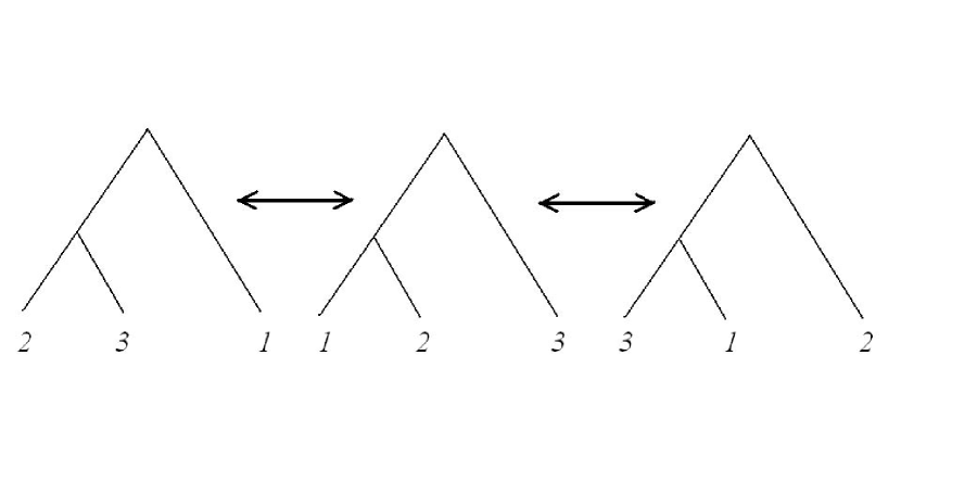
Figure 1: A graphical representation of the associativity condition. The double arrows indicate that the domains ${\mathcal{D}}[{\bf T}_{i}]$ represented by the respective trees have a common intersection, and that on this intersection, the OPE’s represented by the respective trees coincide. Note that the double arrows are not a transitive relation: The domains associated with left- and rightmost tree have empty intersection.

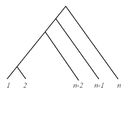
Figure 2: The reference tree $\bf S$.

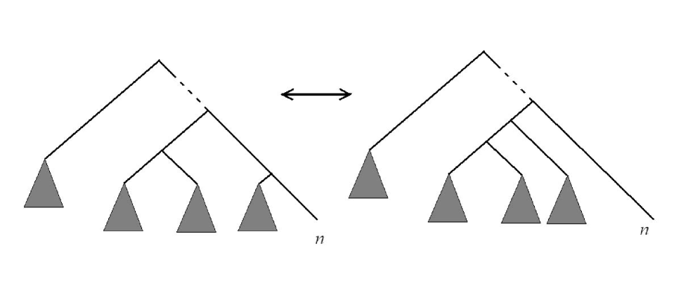
Figure 3: An elementary manipulation. The shaded triangles represent subtrees whose form is not relevant.

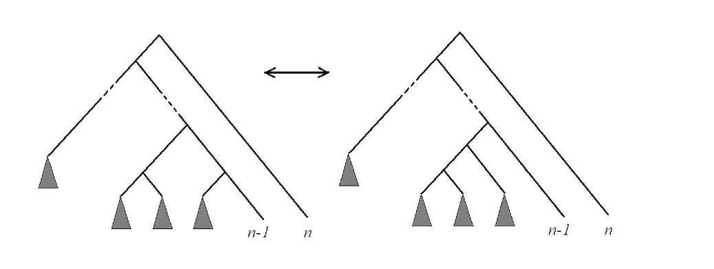
Figure 4: Another elementary manipulation.

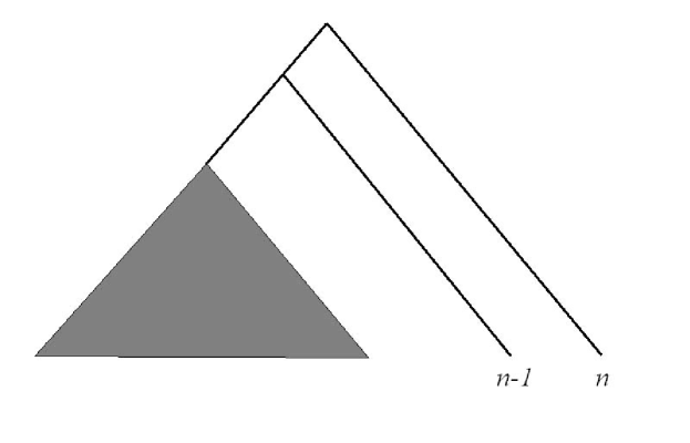
Figure 5: The tree ${\bf T}_{r_{2}}$.

We summarize our finding in the following theorem:

Theorem 1.

(”Coherence Theorem”) For each binary tree ${\bf T}$, let $f_{\bf T}$ be defined by eq. (4.53) on the domain ${\mathcal{D}}[{\bf T}]$ as a convergent power series expansion, and assume that $f_{\bf T}$ has an analytic extension to all of $M_{n}$. Furthermore, assume that the associativity condition (4.48) and symmetry and normalization conditions (4.49), (4.50) hold, i.e. that all $f_{\bf T}$ coincide for trees with three leaves. Then $f_{\bf T}=f_{\bf S}$ for any pair of binary trees ${\bf S},{\bf T}$.

5 Perturbations and Hochschild cohomology

Suppose we are given a quantum field theory in terms of OPE-coefficients as described in sec. 3. In this section we discuss the question how to describe perturbations of such a quantum field theory. According to our definition of a quantum field theory, a perturbed quantum field theory should correspond to a perturbation series in some parameter $\lambda$ for the OPE coefficients. Because our axioms for the OPE coefficients imply constraints–especially the factorization axiom–the perturbations of the coefficients will also have to satisfy corresponding constraints. In this section, we will show that these constraints are of a cohomological nature.

As we have discussed, our definition of quantum field theory is algebraic. In fact, as argued in sec. 4, up to technicalities related to the convergence of various series, the constraints on the OPE coefficients can be formulated in the form of an ”associativity condition” for the 2-point OPE coefficients only, see eq. (4.48). Consequently, the perturbed 2-point OPE coefficients will also have to satisfy a corresponding perturbed version of this constraint, and this is in fact essentially the only constraint. It is this perturbed version of the associativity condition that we will discuss in this section.

Our discussion is in close parallel to the well-known characterization of perturbations (”deformations”) of an ordinary finite dimensional algebra, an analogy which we have already emphasized in another context above. We therefore begin by recalling the basic theory of deformations of finite-dimensional algebras [36, 29]. Let ${\bf A}$ be a finite-dimensional algebra (over ${\mathbb{C}}$, say), whose product we denote as usual by ${\bf A}\otimes{\bf A}\to{\bf A},A\otimes B\mapsto AB$. A deformation of the algebra is a 1-parameter family of products $A\otimes B\mapsto A\bullet_{\lambda}B$, where $\lambda\in{\mathbb{R}}$ is a smooth deformation parameter. The product $A\bullet_{0}B$ should be the original product $AB$, but for non-zero $\lambda$, we have a new product on ${\bf A}$—or alternatively on the ring of formal power series ${\mathbb{C}}((\lambda))\otimes{\bf A}$ if we merely consider perturbations in the sense of formal power series. This new product must satisfy the associativity law, which imposes a strong constraint. If we denote the $i$-th order perturbation of the product by

$$m_{i}(A,B)=\frac{1}{i!}\,\frac{d^{i}}{d\lambda^{i}}A\bullet_{\lambda}B\Bigg{|}_{\lambda=0}\,,$$ (5.55)

then the associativity condition implies to first order that we should have

$$m_{0}(id\otimes m_{1})-m_{0}(m_{1}\otimes id)+m_{1}(id\otimes m_{0})-m_{1}(m_{0}\otimes id)=0\,,$$ (5.56)

as a map ${\bf A}\otimes{\bf A}\otimes{\bf A}\to{\bf A}$, in an obvious tensor product notation. $m_{0}(A,B)=AB$ is the original product on ${\bf A}$. Similar conditions arise for the higher derivatives $m_{i}$ of the new product. These may be written for $i\geq 2$ as

$$m_{0}(id\otimes m_{i})-m_{0}(m_{i}\otimes id)+m_{i}(id\otimes m_{0})-m_{i}(m_{0}\otimes id)$$ (5.57)

$$= -\sum_{j=1}^{i-1}m_{i-j}(id\otimes m_{j})-m_{i-j}(m_{j}\otimes id)\,.$$

Actually, we want to exclude the trivial case that the new product was obtained from the old one by merely a $\lambda$-dependent redefinition of the generators of ${\bf A}$. Such a redefinition may be viewed as a 1-parameter family of invertible linear maps $\alpha_{\lambda}:{\bf A}\to{\bf A}$, and the corresponding trivially deformed product is

$$A\bullet_{\lambda}B=\alpha_{\lambda}^{-1}\Big{[}\alpha_{\lambda}(A)\alpha_{\lambda}(B)\Big{]}\,.$$ (5.58)

In other words, $\alpha_{\lambda}$ defines an isomorphism between $({\bf A},\bullet_{0})$ and $({\bf A},\bullet_{\lambda})$, meaning that the latter should not be regarded as a new algebra. The trivially deformed product is given to first order by

$$m_{1}=m_{0}(id\otimes\alpha_{1})+m_{0}(\alpha_{1}\otimes id)-\alpha_{1}m_{0}\,,$$ (5.59)

with similar formulas for $m_{i}$, where $\alpha_{i}=\frac{1}{i!}\,\frac{d^{i}}{d\lambda^{i}}\alpha_{\lambda}|_{\lambda=0}$.

The above conditions for the $i$-th order deformations of an associative product have a useful and elegant cohomological interpretation [36]. To give this interpretation, consider the linear space $\Omega^{n}({\bf A})$ of all linear maps $\psi_{n}:{\bf A}\otimes\dots\otimes{\bf A}\to{\bf A}$, and define a linear operator $d:\Omega^{n}\to\Omega^{n+1}$ by the formula

$$(d\psi_{n})(A_{1},\dots,A_{n+1}) = A_{1}\psi_{n}(A_{2},\dots,A_{n+1})-(-1)^{n}\psi_{n}(A_{1},\dots,A_{n})A_{n+1}$$ (5.60)

$$+\sum_{j=1}^{n}(-1)^{j}\psi_{n}(A_{1},\dots,A_{j}A_{j+1},\dots,A_{n+1})\,.$$

It may be checked using the associativity law for the original product on the algebra ${\bf A}$ that $d^{2}=0$, so $d$ is a differential with a corresponding cohomology complex. This complex is called the Hochschild complex, see e.g. [30]. More precisely, if $Z^{n}({\bf A})$ is the space of all closed $\psi_{n}$, i.e., those satisfying $d\psi_{n}=0$, and $B^{n}({\bf A})$ the space of all exact $\psi_{n}$, i.e., those for which $\psi_{n}=d\psi_{n-1}$ for some $\psi_{n-1}$, then the $n$-th Hochschild cohomology $HH^{n}({\bf A})$ is defined as the quotient $Z^{n}({\bf A})/B^{n}({\bf A})$. The first order associativity condition may now be viewed as saying that $dm_{1}=0$, or $m_{1}\in Z^{2}({\bf A})$. Furthermore, if the new product just arises from a trivial redefinition of the generators in the sense of (5.58), then it follows that $m_{1}=d\alpha_{1}$, so $m_{1}\in B^{2}({\bf A})$ in that case. Thus, the non-trivial first order perturbations $m_{1}$ of the algebra product can be identified with the non-trivial classes $[m_{1}]\in HH^{2}({\bf A})$. In particular, non-trivial deformations may only exist if $HH^{2}({\bf A})\neq 0$. Let us assume a non-trivial first order perturbation exists, and let us try to find a second order perturbation. We view the right side of the second order associativity condition as an element $w_{2}\in\Omega^{3}({\bf A})$, and we compute that $dw_{2}=0$, so $w_{2}\in Z^{3}({\bf A})$. Actually, the left side of the second order associativity condition is just $dm_{2}\in B^{3}({\bf A})$ in our cohomological notation, so if the second order associativity condition is to hold, then $w_{2}$ must in fact be an element of $B^{3}({\bf A})$, or equivalently, the class $[w_{2}]\in HH^{3}({\bf A})$ must vanish. If it does not define the trivial class—as may only happen if $HH^{3}({\bf A})\neq 0$ itself is non-trivial—then there is an obstruction to lift the perturbation to second order. If there is no obstruction at second order, we continue to third order, with a corresponding potential obstruction $[w_{3}]\in HH^{3}({\bf A})$, and so on. In summary, the space of non-trivial perturbations corresponds to elements of $HH^{2}({\bf A})$, while the obstructions lie in $HH^{3}({\bf A})$.

We now show how to give a similar characterization of perturbations of a quantum field theory. According to our definition of a quantum field theory given in sec. 3, a quantum field theory is defined by the set of its OPE-coefficients with certain properties. Furthermore, as argued in sec. 4, all higher $n$-point operator product coefficients are uniquely determined by the 2-point coefficients ${\cal C}(x_{1},x_{2})$. Furthermore, we argued that, up to technical assumptions about the convergence of the series (4.53), the key constraints on the OPE coefficients for $n$ points are encoded in the associativity constraint (4.48) for the 2-point coefficient, which we repeat for convenience:

$${\cal C}(x_{2},x_{3})\Big{(}{\cal C}(x_{1},x_{2})\otimes id\Big{)}-{\cal C}(x_{1},x_{3})\Big{(}id\otimes{\cal C}(x_{2},x_{3})\Big{)}=0\quad\text{for $r_{12}<r_{23}<r_{13}$.}$$ (5.61)

We ask the question when it is possible to find a 1-parameter deformation ${\cal C}(x_{1},x_{2};\lambda)$ of these coefficients by a parameter $\lambda$ so that the associativity condition continues to hold, at least in the sense of formal power series in $\lambda$. Actually, the analogues of the symmetry condition (4.49), the normalization condition (4.50), the hermitian conjugation, the Euclidean invariance, and the unit axiom should hold as well for the perturbation. However, these conditions are much more trivial in nature than (5.61), because these conditions are linear in ${\cal C}(x_{1},x_{2})$. These conditions could therefore easily be included in our discussion, but would distract from the main point. For the rest of this section, we will therefore discuss the implications of the associativity condition (5.61) for the perturbed OPE-coefficients.

As we shall see now, such perturbations can again be characterized in a cohomological framework similar to the one given above. As above, we will presently define a linear operator $b$ which defines the cohomology in question. The definition of this operator will implicitly involve infinite sums [as our associativity condition (5.61)], and such sums are typically only convergent on certain domains. It is therefore necessary to get a set of domains that will be stable under the action of $b$ and that is suitable for our application. Many such domains can be defined, and correspondingly different rings are obtained. For simplicity and definiteness, we consider the non-empty, open domains of $({\mathbb{R}}^{D})^{n}$ defined by

$${\mathcal{F}}_{n}=\{(x_{1},\dots,x_{n})\in M_{n};\,\,\,r_{1\,i-1}<r_{i-1\,i}<r_{i-2\,i}<\dots<r_{1i},\,\,\,1<i\leq n\}\subset M_{n}\,.$$ (5.62)

These domains also have a description in terms of the domains ${\mathcal{D}}[{\bf T}]$ defined above in eq. (4.51), but we will not need this here. Note that the associativity condition (5.61) holds on the domain ${\mathcal{F}}_{3}=\{r_{12}<r_{23}<r_{13}\}$.

We define $\Omega^{n}(V)$ to be the set of all holomorphic functions $f_{n}$ on the domain ${\mathcal{F}}_{n}$ that are valued in the linear maps 

$$f_{n}(x_{1},\dots,x_{n}):V\otimes\dots\otimes V\to V,\quad(x_{1},\dots,x_{n})\in{\mathcal{F}}_{n}\,.$$ (5.63)

We next introduce a boundary operator $b:\Omega^{n}(V)\to\Omega^{n+1}(V)$ by the formula

$$(bf_{n})(x_{1},\dots,x_{n+1}):={\cal C}(x_{1},x_{n+1})(id\otimes f_{n}(x_{2},\dots,x_{n+1}))$$

$$+\sum_{i=1}^{n}(-1)^{i}f_{n}(x_{1},\dots,\widehat{x}_{i},\dots,x_{n+1})(id^{i-1}\otimes{\cal C}(x_{i},x_{i+1})\otimes id^{n-i})$$

$$+(-1)^{n+1}\,{\cal C}(x_{n},x_{n+1})(f_{n}(x_{1},\dots,x_{n})\otimes id)\,.$$ (5.64)

Here ${\cal C}(x_{1},x_{2})$ is the OPE-coefficient of the undeformed theory and a caret means omission. The definition of $b$ involves a composition of ${\cal C}$ with $f_{n}$, and hence, when expressed in a basis of $V$, implicitly involves an infinite summation over the basis elements of $V$. We must therefore assume here (and in similar formulas in the following) that these sums converge on the set of points $(x_{1},\dots,x_{n+1})$ in the domain ${\mathcal{F}}_{n+1}$. Thus, when we write $bf_{n}$, it is understood that $f_{n}\in\Omega^{n}(V)$ is in the domain of $b$. We now have the following lemma:

Lemma 1.

The maps $b$ is a differential, i.e., $b^{2}f_{n}=0$ for $f_{n}$ in the domain of $b$ such that $bf_{n}$ is also in the domain of $b$.

Proof: The proof is essentially a straightforward computation. Using the definition of $b$, we have

$$b(bf_{n})(x_{1},\dots,x_{n+2})={\cal C}(x_{1},x_{n+2})(id\otimes bf_{n}(x_{2},\dots,x_{n+2}))$$

$$+\sum_{i=1}^{n+1}(-1)^{i}bf_{n}(x_{1},\dots,\widehat{x}_{i},\dots,x_{n+2})(id^{i-1}\otimes{\cal C}(x_{i},x_{i+1})\otimes id^{n+1-i})$$

$$+(-1)^{n+2}{\cal C}(x_{n+1},x_{n+2})(bf_{n}(x_{1},\dots,x_{n+1})\otimes id)\,.$$ (5.65)

Substituting the definition of $b$ again then gives, for the first term on the right side

$$={\cal C}(x_{1},x_{n+2})[id\otimes{\cal C}(x_{2},x_{n+2})(id\otimes f_{n}(x_{3},\dots,x_{n+2}))]$$

$${\cal C}(x_{1},x_{n+2})[id\otimes\sum_{k=2}^{n+1}(-1)^{k-1}f_{n}(x_{2},\dots,\widehat{x}_{k},\dots,x_{n+2})(id^{k-2}\otimes{\cal C}(x_{k},x_{k+1})\otimes id^{n-k+1})]$$

$$+(-1)^{n+1}{\cal C}(x_{1},x_{n+2})[id\otimes{\cal C}(x_{n+1},x_{n+2})(f_{n}(x_{2},\dots,x_{n+1})\otimes id)]\,.$$ (5.66)

Substituting the definition of $b$ into the third term on the right side of eq. (5) gives

$$=(-1)^{n}{\cal C}(x_{n+1},x_{n+2})[{\cal C}(x_{1},x_{n+1})(id\otimes f_{n}(x_{2},\dots,x_{n+1}))\otimes id]$$

$$+(-1)^{n}{\cal C}(x_{n+1},x_{n+2})[\sum_{i=1}^{n}(-1)^{i}f_{n}(x_{1},\dots,\widehat{x}_{i},\dots,x_{n+1})(id^{i-1}\otimes{\cal C}(x_{i},x_{i+1})\otimes id^{n-i})\otimes id]$$

$$-{\cal C}(x_{n+1},x_{n+2})[{\cal C}(x_{n},x_{n+1})(f_{n}(x_{1},\dots,x_{n})\otimes id)\otimes id]\,.$$ (5.67)

Substituting the definition of $b$ into the second term on the right side of eq. (5) gives the following terms

$$=\sum_{i=2}^{n+1}(-1)^{i}{\cal C}(x_{1},x_{n+2})[id\otimes f_{n}(x_{2},\dots,\widehat{x}_{i},\dots,x_{n+2})(id^{i-1}\otimes{\cal C}(x_{i},x_{i+1})\otimes id^{n+1-i})]$$

$$-{\cal C}(x_{2},x_{n+2})(id\otimes f_{n}(x_{3},\dots,x_{n+2}))({\cal C}(x_{1},x_{2})\otimes id^{n})$$

$$+\sum_{i=1}^{n}(-1)^{i+n+1}{\cal C}(x_{n+1},x_{n+2})[(f_{n}(x_{1},\dots,\widehat{x}_{i},\dots,x_{n+1})\otimes id)(id^{i-1}\otimes{\cal C}(x_{i},x_{i+1})\otimes id^{n-i+1})]$$

$$+{\cal C}(x_{n},x_{n+2})(f_{n}(x_{1},\dots,x_{n})\otimes id)(id^{n}\otimes{\cal C}(x_{n+1},x_{n+2}))$$

$$+\sum_{k=2}^{n}\sum_{i=1}^{k-1}(-1)^{k+i}f_{n}(x_{1},\dots,\widehat{x}_{i},\dots,\widehat{x}_{k+1},\dots,x_{n+2})\circ$$

$$\quad\circ(id^{k-1}\otimes{\cal C}(x_{k+1},x_{k+2})\otimes id^{n-k})(id^{i-1}\otimes{\cal C}(x_{i},x_{i+1})\otimes id^{n-i+1})$$

$$+\sum_{k=1}^{n-1}\sum_{i=k+2}^{n+1}(-1)^{k+i}f_{n}(x_{1},\dots,\widehat{x}_{k},\dots,\widehat{x}_{i},\dots,x_{n+2})\circ$$

$$\quad\circ(id^{k-1}\otimes{\cal C}(x_{k},x_{k+1})\otimes id^{n-k})(id^{i-1}\otimes{\cal C}(x_{i},x_{i+1})\otimes id^{n-i+1})$$

$$-\sum_{k=1}^{n}f_{n}(x_{1},\dots,\widehat{x}_{k},\widehat{x}_{k+1},\dots,x_{n+2})\circ$$

$$\quad\circ(id^{k-1}\otimes{\cal C}(x_{k},x_{k+2})\otimes id^{n-k})(id^{k}\otimes{\cal C}(x_{k+1},x_{k+2})\otimes id^{n-k})$$

$$+\sum_{k=1}^{n}f_{n}(x_{1},\dots,\widehat{x}_{k},\widehat{x}_{k+1},\dots,x_{n+2})\circ$$

$$\quad\circ(id^{k-1}\otimes{\cal C}(x_{k+1},x_{k+2})\otimes id^{n-k})(id^{k-1}\otimes{\cal C}(x_{k},x_{k+1})\otimes id^{n-k+1})\,.$$ (5.68)

We now add up the expressions that we have obtained, and we use the associativity condition eq. (5.61), noting that we are allowed to use this expression on the domain ${\mathcal{F}}_{n+2}$: For example, to apply the associativity condition to the last two terms in the above expression, we need that $r_{k\,k+1}<r_{k+1\,k+2}<r_{k\,k+2}$ for all $k$, which holds on ${\mathcal{F}}_{n+2}$. It is this property of the domains ${\mathcal{F}}_{i}$ that motivates our definition (5.62). Applying the associativity condition, we find that all terms cancel, thus proving the lemma. ∎

By this lemma, we can define a cohomology ring associated with the differential $b$ as

$$H^{n}(V;{\cal C}):=\frac{Z^{n}(V;{\cal C})}{B^{n}(V;{\cal C})}=\frac{\{{\rm ker}\,b:\Omega^{n}(V)\to\Omega^{n+1}(V)\}}{\{{\rm ran}\,b:\Omega^{n-1}(V)\to\Omega^{n}(V)\}}\,.$$ (5.69)

As we will now see, the problem of finding a 1-parameter family of perturbations ${\cal C}(x_{1},x_{2};\lambda)$ such that our associativity condition (5.61) continues to hold for ${\cal C}(x_{1},x_{2};\lambda)$ to all orders in $\lambda$ can be elegantly and compactly be formulated in terms of this ring. If we let

$${\cal C}_{i}(x_{1},x_{2})=\frac{1}{i!}\,\frac{d^{i}}{d\lambda^{i}}{\cal C}(x_{1},x_{2};\lambda)\Bigg{|}_{\lambda=0}\,,$$ (5.70)

then we note that the first order associativity condition,

$${\cal C}_{0}(x_{2},x_{3})\Big{(}{\cal C}_{1}(x_{1},x_{2})\otimes id\Big{)}-{\cal C}_{0}(x_{1},x_{3})\Big{(}id\otimes{\cal C}_{1}(x_{2},x_{3})\Big{)}+$$

$${\cal C}_{1}(x_{2},x_{3})\Big{(}{\cal C}_{0}(x_{1},x_{2})\otimes id\Big{)}-{\cal C}_{1}(x_{1},x_{3})\Big{(}id\otimes{\cal C}_{0}(x_{2},x_{3})\Big{)}=0\,\,,$$ (5.71)

valid for $(x_{1},x_{2},x_{3})\in{\mathcal{F}}_{3}$, is equivalent to the statement that

$$b{\cal C}_{1}=0\,,$$ (5.72)

where here and in the following, $b$ is defined in terms of the unperturbed OPE-coefficient ${\cal C}_{0}$. Thus, ${\cal C}_{1}$ has to be an element of $Z^{2}(V;{\cal C}_{0})$. Let $z(\lambda):V\to V$ be a $\lambda$-dependent field redefinition in the sense of defn. 3.1, and suppose that ${\cal C}(x_{1},x_{2})$ and ${\cal C}(x_{1},x_{2};\lambda)$ are connected by the field redefinition. To first order, this means that

$${\cal C}_{1}(x_{1},x_{2})=-z_{1}{\cal C}_{0}(x_{1},x_{2})+{\cal C}_{0}(x_{1},x_{2})(z_{1}\otimes id+id\otimes z_{1})\,,$$ (5.73)

or equivalently, that $bz_{1}={\cal C}_{1}$, where $z_{i}=\frac{1}{i!}\,\frac{d^{i}}{d\lambda^{i}}z(\lambda)|_{\lambda=0}$. Thus, the first order deformations of ${\cal C}_{0}$ modulo the trivial ones defined by eq. (5.73) are given by the classes in $H^{2}(V;{\cal C}_{0})$. The associativity condition for $i$-th order perturbation (assuming that all perturbations up to order $i-1$ exist) can be written as the following condition for $(x_{1},x_{2},x_{3})\in{\mathcal{F}}_{3}$:

$${\cal C}_{0}(x_{2},x_{3})\Big{(}{\cal C}_{j}(x_{1},x_{2})\otimes id\Big{)}-{\cal C}_{j}(x_{1},x_{3})\Big{(}id\otimes{\cal C}_{0}(x_{2},x_{3})\Big{)}+$$ (5.74)

$${\cal C}_{j}(x_{2},x_{3})\Big{(}{\cal C}_{0}(x_{1},x_{2})\otimes id\Big{)}-{\cal C}_{0}(x_{1},x_{3})\Big{(}id\otimes{\cal C}_{j}(x_{2},x_{3})\Big{)}=w_{i}(x_{1},x_{2},x_{3})\,,$$

where $w_{i}\in\Omega^{3}(V)$ is defined by

$$w_{i}(x_{1},x_{2},x_{3}):=-\sum_{j=1}^{i-1}{\cal C}_{i-j}(x_{1},x_{3})(id\otimes{\cal C}_{j}(x_{2},x_{3}))-{\cal C}_{i-j}(x_{2},x_{3})({\cal C}_{j}(x_{1},x_{2})\otimes id)\,.$$ (5.75)

We assume here that all infinite sums implicit in this expression converge on ${\mathcal{F}}_{3}$. This equation may be written alternatively as

$$b{\cal C}_{i}=w_{i}\,.$$ (5.76)

We would like to define the $i$-th order perturbation by solving this linear equation for ${\cal C}_{i}$. Clearly, a necessary condition for there to exist a solution is that $bw_{i}=0$ or $w_{i}\in Z^{3}(V,{\cal C}_{0})$, and this can indeed shown to be the case, see lemma 2 below. If a solution to eq. (5.76) exists, i.e. if $w_{i}\in B^{3}(V,{\cal C}_{0})$, then any other solution will differ from this one by a solution to the corresponding ”homogeneous” equation. Trivial solutions to the homogeneous equation of the form $bz_{i}$ again correspond to an $i$-th order field redefinition and are not counted as genuine perturbations. In summary, the perturbation series can be continued at $i$-th order if $[w_{i}]$ is the trivial class in $H^{3}(V;{\cal C}_{0})$, so $[w_{i}]$ represents a potential $i$-th order obstruction to continue the perturbation series. If there is no obstruction, then the space of non-trivial $i$-th order perturbations is given by $H^{2}(V;{\cal C}_{0})$. In particular, if we knew e.g. that $H^{2}(V;{\cal C}_{0})\neq 0$ while $H^{3}(V;{\cal C}_{0})=0$, then perturbations could be defined to arbitrary orders in $\lambda$.

Lemma 2.

If $w_{i}$ is in the domain of $b$, and if $b{\cal C}_{j}=w_{j}$ for all $j<i$, then $bw_{i}=0$.

Proof: We proceed by induction in $i$. For $i=1$, the lemma is true as we have $w_{1}=b{\cal C}_{1}$, so $bw_{1}=0$ by $b^{2}=0$. In the general case, using the definition of $b$, we obtain the following expression for $bw_{i}$:

$$-bw_{i}(x_{1},x_{2},x_{3},x_{4})$$ (5.77)

$$=\sum_{j=1}^{i-1}{\cal C}_{0}(x_{1},x_{4})\Big{(}id\otimes{\cal C}_{j}(x_{2},x_{4})(id\otimes{\cal C}_{i-j}(x_{3},x_{4}))\Big{)}$$

$$-\sum_{j=1}^{i-1}{\cal C}_{j}(x_{2},x_{4})\Big{(}id\otimes{\cal C}_{i-j}(x_{3},x_{4})\Big{)}\Big{(}{\cal C}_{0}(x_{1},x_{2})\otimes id^{2}\Big{)}$$

$$+\sum_{j=1}^{i-1}{\cal C}_{j}(x_{1},x_{4})\Big{(}id\otimes{\cal C}_{i-j}(x_{3},x_{4})\Big{)}\Big{(}id\otimes{\cal C}_{0}(x_{2},x_{3})\otimes id\Big{)}$$

$$-\sum_{j=1}^{i-1}{\cal C}_{j}(x_{1},x_{4})\Big{(}id\otimes{\cal C}_{i-j}(x_{2},x_{4})\Big{)}\Big{(}id^{2}\otimes{\cal C}_{0}(x_{3},x_{4})\Big{)}$$

$$+\sum_{j=1}^{i-1}{\cal C}_{0}(x_{3},x_{4})\Big{(}{\cal C}_{j}(x_{1},x_{3})(id\otimes{\cal C}_{i-j}(x_{2},x_{3}))\otimes id\Big{)}$$

$$-\sum_{j=1}^{i-1}{\cal C}_{0}(x_{1},x_{4})\Big{(}id\otimes{\cal C}_{j}(x_{3},x_{4})({\cal C}_{i-j}(x_{2},x_{3})\otimes id)\Big{)}$$

$$+\sum_{j=1}^{i-1}{\cal C}_{j}(x_{3},x_{4})\Big{(}{\cal C}_{i-j}(x_{2},x_{3})\otimes id\Big{)}\Big{(}{\cal C}_{0}(x_{1},x_{2})\otimes id^{2}\Big{)}$$

$$-\sum_{j=1}^{i-1}{\cal C}_{j}(x_{3},x_{4})\Big{(}{\cal C}_{i-j}(x_{1},x_{3})\otimes id\Big{)}\Big{(}id\otimes{\cal C}_{0}(x_{2},x_{3})\otimes id\Big{)}$$

$$+\sum_{j=1}^{i-1}{\cal C}_{j}(x_{2},x_{4})\Big{(}{\cal C}_{i-j}(x_{1},x_{2})\otimes id\Big{)}\Big{(}id^{2}\otimes{\cal C}_{0}(x_{3},x_{4})\Big{)}$$

$$-\sum_{j=1}^{i-1}{\cal C}_{0}(x_{3},x_{4})\Big{(}{\cal C}_{j}(x_{2},x_{3})({\cal C}_{i-j}(x_{1},x_{2})\otimes id)\otimes id\Big{)}\,.$$

After some manipulations using the definition of $b$ and that by definition the points $(x_{1},x_{2},x_{3},x_{4})$ are assumed to be in ${\mathcal{F}}_{4}$, we can transform this into the following expression

$$-bw_{i}(x_{1},x_{2},x_{3},x_{4})$$

$$= +\sum_{j=1}^{i-1}b{\cal C}_{j}(x_{1},x_{2},x_{4})(id^{2}\otimes{\cal C}_{i-j}(x_{3},x_{4}))$$

$$-\sum_{j=1}^{i-1}{\cal C}_{j}(x_{1},x_{4})(id\otimes b{\cal C}_{i-j}(x_{2},x_{3},x_{4}))$$

$$-\sum_{j=1}^{i-1}b{\cal C}_{j}(x_{1},x_{3},x_{4})(id\otimes{\cal C}_{i-j}(x_{2},x_{3})\otimes id)$$

$$-\sum_{j=1}^{i-1}{\cal C}_{j}(x_{3},x_{4})(b{\cal C}_{i-j}(x_{1},x_{2},x_{3})\otimes id)$$

$$+\sum_{j=1}^{i-1}b{\cal C}_{j}(x_{2},x_{3},x_{4})({\cal C}_{i-j}(x_{1},x_{2})\otimes id^{2})\,,$$

where the first sum comes from the first two sums of the previous equation, the second from the third and fourth two sums, etc. We now substitute the relation $b{\cal C}_{j}=w_{j}$ for $j\leq i-1$ on ${\mathcal{F}}_{3}$, noting that we are allowed to do so when $(x_{1},x_{2},x_{3},x_{4})\in{\mathcal{F}}_{4}$: For example, in the last term $(x_{2},x_{3},x_{4})\in{\mathcal{F}}_{3}$ is satisfied whenever $(x_{1},x_{2},x_{3},x_{4})\in{\mathcal{F}}_{4}$, and a similar statement holds for the other 4 terms [this is in fact our motivation for our definition of the domains ${\mathcal{F}}_{n}$]. We then perform the sum over $j$. If this is done, then we see that the five terms in the sum become ten terms involving each three factors of the ${\cal C}$’s. These terms cancel pairwise, and we get the desired result that $bw_{i}=0$, as we desired to show. ∎

6 Gauge Theories

Local gauge theories are typically more complicated than theories without local gauge invariance. One way to understand the complicating effects due to local gauge invariance is to realize that the dynamical field equations are not hyperbolic in nature in Lorentzian spacetimes. This is seen most clearly in the case of classical field theories. Because local gauge transformations may be used to change the gauge connection in arbitrary compact regions of spacetime, it is clear that the gauge connection cannot be entirely determined by the dynamical equations and its initial data on some spatial time slice. Thus, there is no well-posed initial value formulation in the standard sense. Similar remarks apply to the Euclidean situation.

To circumvent this problem, one typically proceeds in two steps. At the first step, an auxiliary theory is considered, containing the gauge fields as well as additional ”ghost” fields taking values in an infinite-dimensional Grassmann algebra. This theory has a well-posed initial value formulation. At the second step, the new degrees of freedom are removed. Here it is important that the auxiliary theory possesses a new symmetry, the so-called BRST-symmetry, $s$, which is a linear transformation on the space of classical fields with the property $s^{2}=0$ [for example, in Yang-Mills theory $s$ is given by eq. (2.9)]. It turns out that the field content and dynamics of the original theory may be recovered by considering only the equivalence classes of fields in the auxiliary theory that are in the null-space of $s$, modulo those that are in the range of $s$. Thus, the second step is to define the observables of the gauge theory in question as the cohomology of the ”differential” $s$.

At the quantum level, one has a similar structure. In the framework considered in this paper, the situation may be described abstractly as follows: As before, we have an abstract vector space of fields, $V$. This space is to be thought of as the collection of the components of all (composite) fields in the auxiliary theory including ghost fields. The space $V$ is equipped with a grading $\gamma$ and a differential $s$, i.e., two linear maps

$$s:V\to V\,,\quad\gamma:V\to V\,,$$ (6.79)

with the properties

$$s^{2}=0\,,\quad\gamma^{2}=id\,\quad\gamma s+s\gamma=0\,.$$ (6.80)

The map $s$ should be thought of as being analogous to the classical BRST-transformation. The map $\gamma$ has eigenvalues $\pm 1$, and the eigenvectors correspond as above to Bose/Fermi fields. At the classical level, the elements in the eigenspace of $-1$ are analogous to the classical (composite) fields of odd Grassmann parity, while those in the eigenspace of $+1$ are analogous to those of even Grassmann parity. However, we emphasize that these are just analogies, as we will be dealing with a quantum field theory. For the general analysis of quantum gauge theories we will only need $s$ and $\gamma$ to satisfy the above properties. It is also natural to postulate the existence of another grading map $g:V\to V$ with the properties ${\rm Spec}\,g=\mathbb{Z}$ and $sg=(g+id)s$, $\gamma g-g\gamma=0$. This map is to be thought of as the number counter for the ghost fields (so that $s$ increases the ghost number by one unit). Finally, we would like all maps $s,\gamma,g$ to be compatible with the $\star$-operation on $V$, and to preserve the grading by the spin, as well as the dimension.

We next consider a quantum field theory whose fields are described by the elements of $V$, with operator product coefficients ${\cal C}$. At the classical level, $s$ is a graded derivation, so we would also like $s$ to be a graded derivation at the quantum level. Recall that if ${\bf A}$ is a graded algebra with grading map $\Gamma$ (i.e., $\Gamma^{2}=id$), then a graded derivation is a map $D:{\bf A}\to{\bf A}$ with the property that

$$D(AB)=(DA)B+\Gamma(A)DB\quad\text{for all $A,B\in{\bf A}$}\,.$$ (6.81)

Equivalently, if we write the product in the algebra as $m:{\bf A}\otimes{\bf A}\to{\bf A}$ with $m(A,B)=AB$, then $m$ should satisfy

$$Dm=m(D\otimes id)+m(\Gamma\otimes D)\,,$$ (6.82)

in the sense of maps ${\bf A}\otimes{\bf A}\to{\bf A}$. As we have emphasized several times, the OPE-coefficients ${\cal C}(x_{1},x_{2})$ are to be thought of informally as the expansion coefficients of a product. Therefore, if $s$ is to be a graded derivation we should add a corresponding additional axiom to those formulated above in sec. 3. Heuristically, we want $s$ to act on a product of quantum fields $\phi_{a}$ in the following way analogous to eq. (6.81):

$$s\Big{[}\prod_{i=1}^{n}\phi_{a_{i}}(x_{i})\Big{]}=\sum_{i=1}^{n}(-1)^{\sum_{j<i}\epsilon_{i}}\phi_{a_{1}}(x_{1})\cdots s\phi_{a_{i}}(x_{i})\cdots\phi_{a_{n}}(x_{n})\,,$$ (6.83)

Here, $\epsilon_{i}=0,1$ according to whether $\phi_{a_{i}}$ is bosonic or fermionic. If we formally apply an OPE to both sides of this equation, then we arrive at the following condition for the OPE coefficients:

BRST-invariance:

The OPE coefficients of the auxiliary should satisfy the additional condition

$$s{\cal C}(x_{1},\dots,x_{n})=\sum_{i=1}^{n}{\cal C}(x_{1},\dots,x_{n})(\gamma^{i-1}\otimes s\otimes id^{n-i})$$ (6.84)

for all $n$.

Above, we have seen in prop. 1 that the 2-point OPE coefficients determine all higher coefficients uniquely. Thus, as a corollary, the above conditions of $BRST$-invariance will be satisfied if they hold for the 2-point coefficients, i.e. if the condition

$$s{\cal C}(x_{1},x_{2})={\cal C}(x_{1},x_{2})(s\otimes id)+{\cal C}(x_{1},x_{2})(\gamma\otimes s)$$ (6.85)

holds. Furthermore, we would like to formulate abstractly the condition that, since the OPE coefficients are valued in the complex numbers, they should have ”ghost number” equal to zero, meaning that

$$g{\cal C}(x_{1},x_{2})={\cal C}(x_{1},x_{2})(g\otimes id)+{\cal C}(x_{1},x_{2})(id\otimes g)\,.$$ (6.86)

In summary a quantum gauge theory is described in our language abstractly as follows:

Definition 6.1.

A quantum gauge theory is a system of OPE-coefficients

$${\cal C}=({\cal C}(x_{1},x_{2}),{\cal C}(x_{1},x_{2},x_{3}),\dots)$$ (6.87)

associated with $V$ satisfying the properties laid out in sec. 3, together with a ghost number grading $g$ satisfying (6.86), and a differential $s:V\to V$ satisfying (6.85) and (6.80), as well as $(g+id)s=sg$.

By analogy with the classical case, we define the space of physical fields of the gauge theory to be the quotient

$$\widehat{V}:=\frac{\{{\rm ker}\,s:V^{0}\to V^{+1}\}}{\{{\rm ran}\,s:V^{-1}\to V^{0}\}}$$ (6.88)

where $V^{q}$ are the eigenspaces of the linear map $g$, with eigenvalue $q$,

$$V=\bigoplus_{q\in\mathbb{Z}}V^{q}\,,\quad s:V^{q}\to V^{q+1}\,.$$ (6.89)

In other words, we define the space of physical fields as the zeroth cohomology group defined by $s$, with the general cohomology group at $q$-th order defined by

$$H^{q}(V;s)=\frac{\{{\rm ker}\,s:V^{q}\to V^{q+1}\}}{\{{\rm ran}\,s:V^{q-1}\to V^{q}\}}\,.$$ (6.90)

Because the OPE coefficients satisfy the assumption of BRST invariance, eq (6.84), we have the following proposition/definition:

Proposition 2.

The OPE coefficients ${\cal C}$ of the auxiliary theory induce maps

$$\widehat{\cal C}(x_{1},\dots,x_{n}):\widehat{V}\otimes\dots\otimes\widehat{V}\to\widehat{V}\,,$$ (6.91)

so the operator product expansion ”closes” on the space $\widehat{V}$ of physical fields. Therefore, the true physical sector of the gauge theory can be defined as the quantum field theory described by the pair $(\widehat{V},\widehat{\cal C})$.

Remarks:

1) In Yang-Mills theory with Lie algebra $\mathfrak{g}$, the space $V$ is naturally identified with the free unital commutative $\partial_{\mu}$-differential module (over ${\mathbb{C}}[\lambda]$) generated by the formal expressions of the form ${\bf 1}$ and

$$\partial_{\mu_{1}}\dots\partial_{\mu_{k}}\psi_{i};\,\,\mu_{j}=1,\dots,D\,,$$ (6.92)

where $\psi_{i}$ denotes either a component of $A$ or the auxiliary ”field” $F$ or the ghost ”fields”, $U,\bar{U}$. The expressions in $V$ are taken modulo the relations $\psi_{i}\psi_{j}=(-1)^{F_{i}F_{j}}\psi_{j}\psi_{i}$, with $F_{i}=0$ or $=1$ according to whether $g(\psi_{i})=\pm\psi_{i}$, where $g$ is $-1$ on ghost fields $U,\bar{U}$, and $+1$ on $A,F$. Furthermore, on $V$, the linear maps $\partial_{\mu}$ are defined to act as the (ungraded) derivations that are obtained by formally viewing the elements of $V$ as classical fields. On $V$, there also acts the BRST-differential $s$. It is defined to act on the generators of $V$ by eq. (2.9), and it is demanded to anti-commute with the formal derivations $\partial_{\mu}$, i.e.,

$$\partial_{\mu}\in{\rm Der}(V)\,,\quad s\circ\partial_{\mu}=\partial_{\mu}\circ s\,,\quad g\circ\partial_{\mu}=\partial_{\mu}\circ g\,.$$ (6.93)

One can then show [37] that $\widehat{V}$ corresponds precisely to the gauge-invariant monomials of the field strength tensor of the gauge connection and its covariant derivatives, i.e.,

$$\widehat{V}=\Big{\langle}p({\mathcal{D}}^{k_{1}}F,\dots,{\mathcal{D}}^{k_{n}}F);p\in{\rm Inv}({\mathfrak{g}}^{\otimes n},{\mathbb{C}})\Big{\rangle}\,,$$ (6.94)

where ${\rm Inv}(\mathfrak{g}^{\otimes n},{\mathbb{C}})$ is the space of $\mathfrak{g}$-invariant multi-linear forms on Lie-algebra, ${\mathcal{D}}_{\mu}=\partial_{\mu}+i\lambda[A_{\mu},\,.\,]$ is the standard covariant derivative, $F$ is a shorthand for its curvature, $F_{\mu\nu}=[\mathcal{D}_{\mu},\mathcal{D}_{\nu}]$, and ${\mathcal{D}}^{k}$ is a shorthand for ${\mathcal{D}}_{(\mu_{1}}\cdots{\mathcal{D}}_{\mu_{k})}$.

2) Note that the OPE-coefficients of the auxiliary theory not only close on the space $\widehat{V}$, but more generally on any of the spaces $W_{k}=\oplus_{q\geq k}H^{q}(V;s)$. These spaces contain also operators of non-zero ghost number. One does not, however, expect this theory to have any non-trivial states satisfying the OS-positivity axiom [see sec. 3].

Proof: Let $|v_{1}\rangle,\dots,|v_{n}\rangle\in{\rm ker}\,s$. Using eq. (6.84), we have

$$s\Big{(}{\cal C}(x_{1},\dots,x_{n})|v_{1}\otimes\dots\otimes v_{n}\rangle\Big{)}$$

$$= \sum_{i=1}^{n}{\cal C}(x_{1},\dots,x_{n})|\gamma(v_{1})\otimes\dots\gamma(v_{i-1})\otimes sv_{i}\otimes v_{i+1}\otimes\dots v_{n}\rangle=0\,.$$

Thus, the composition ${\cal C}(x_{1},\dots,x_{n})|v_{1}\otimes\dots\otimes v_{n}\rangle$ is in the kernel of $s$. One similarly shows that if $|v_{1}\rangle,\dots,|v_{n}\rangle\in{\rm ker}\,s$, and in addition $|v_{i}\rangle\in{\rm ran}\,s$ for some $i$, then the composition is even in the image of $s$. Thus, ${\cal C}(x_{1},\dots,x_{n})$ gives a well defined map from $({\rm ker}\,s/{\rm ran}\,s)^{\otimes n}$ into ${\rm ker}\,s/{\rm ran}\,s$. Finally, since ${\cal C}(x_{1},\dots,x_{n})$ satisfies the analogue of eq. (6.86), it follows that the composition has ghost number zero if each $|v_{i}\rangle$ has. Thus, ${\cal C}(x_{1},\dots,x_{n})$ gives a well defined map $\widehat{\cal C}(x_{1},\dots,x_{n})$ from $\widehat{V}^{\otimes n}$ to $\widehat{V}$. This map inherits the properties of factorization, scaling, the unity axiom, the symmetry property etc. from the map ${\cal C}(x_{1},\dots,x_{n})$. Thus, the collection $(\widehat{\cal C},\widehat{V})$ again defines a quantum field theory in our sense. ∎

We would now like to consider perturbations of a given quantum gauge theory by analogy with the procedure described in the previous section. Thus, as above, let $\lambda$ be a formal expansion parameter, and let ${\cal C}(x_{1},x_{2};\lambda)$ be a 1-parameter family describing a deformation of the given 2-point OPE coefficient of the auxiliary theory. As above let $({\cal C}_{0},{\cal C}_{1},{\cal C}_{2},\dots)$ be the zeroth, first, second, etc. perturbations of the expansion coefficients. In order that the perturbed coefficients satisfy the associativity constraint, the equations (5.74) must again hold for the coefficients. In the situation at hand, we also should consider a deformation $s(\lambda)$ of the BRST-differential, with expansion coefficients $(s_{0},s_{1},s_{2},\dots)$,

$$s_{i}=\frac{1}{i!}\,\frac{d^{i}}{d\lambda^{i}}\,s(\lambda)\Bigg{|}_{\lambda=0}\,.$$ (6.96)

These quantities should satisfy the perturbative version of eq. (6.80), that is

$$\sum_{j=0}^{i}s_{j}s_{i-j}=0\,,\quad s_{i}\gamma+\gamma s_{i}=0\,,$$ (6.97)

and they should satisfy the perturbative version of eq. (6.85),

$$\sum_{j=0}^{i}s_{j}{\cal C}_{i-j}(x_{1},x_{2})=\sum_{j=0}^{i}{\cal C}_{i-j}(x_{1},x_{2})(s_{j}\otimes id)+\sum_{j=0}^{i}{\cal C}_{i-j}(x_{1},x_{2})(\gamma\otimes s_{j})\,,$$ (6.98)

for all $i=0,1,2,\dots$. For $i=0$, these conditions are just the conditions that the undeformed theory described by $s_{0},{\cal C}_{0}$ defines a gauge theory. For $i=1,2,\dots$, we get a set of conditions that constrain the possible $i$-th order perturbations $s_{i},{\cal C}_{i}$. Actually, as in the previous section, we would like to exclude again that our deformations $s_{i},{\cal C}_{i}$ are simply due to a $\lambda$-dependent field redefinition, see defn. 3.1. In the present context, a first order perturbation $s_{1},{\cal C}_{1}$ that is simply due to a field redefinition is one for which

$${\cal C}_{1}(x_{1},x_{2})=-z_{1}\,{\cal C}_{0}(x_{1},x_{2})+{\cal C}_{0}(x_{1},x_{2})(z_{1}\otimes id+id\otimes z_{1})\,,\quad s_{1}=s_{0}\,z_{1}+z_{1}\,s_{0}\,,$$ (6.99)

for some $z_{1}:V\to V$ such that $z_{1}\,\gamma=\gamma\,z_{1}$. There are similar conditions at higher order. We will now see that the higher order conditions, have an elegant formulation in terms of a variant of Hochschild cohomology associated with ${\cal C}_{0}$, twisted with the cohomology of $s_{0}$.

In order to describe this, we begin by defining the respective cohomology rings. Our first task is the definition of the Hochschild type differential $b$ in the case when $V$ is a graded vector space. Let ${\cal C}(x_{1},x_{2}):V\otimes V\to V$ satisfy the associativity condition (5.61) and be even under our grading $\gamma$, meaning ${\cal C}(x_{1},x_{2})(\gamma\otimes\gamma)=\gamma{\cal C}(x_{1},x_{2})$.

Definition 6.2.

Let $\Omega^{n}(V)$ be the space of all translation invariant analytic maps $f_{n}:{\mathcal{F}}_{n}\to\hom(V\otimes\dots\otimes V,V)$, where ${\mathcal{F}}_{n}\subset({\mathbb{R}}^{D})^{n}$ is the domain (5.62). Let

$$f^{\gamma}_{n}:=\gamma f_{n}(\gamma\otimes\dots\otimes\gamma)\,.$$ (6.100)

If $f_{n}^{\gamma}=f_{n}$, then $f_{n}$ is said to be even and the definition of $bf_{n}\in\Omega^{n+1}(V)$ is as above in eq. (5). If $f_{n}^{\gamma}=-f_{n}$, then $f_{n}$ is said to be odd, and we define

$$(bf_{n})(x_{1},\dots,x_{n+1}) := -{\cal C}(x_{1},x_{n+1})(\gamma\otimes f_{n}(x_{2},\dots,x_{n+1})$$ (6.101)

$$- \sum_{i=1}^{n}(-1)^{i}f_{n}(x_{1},\dots,\widehat{x}_{i},\dots,x_{n+1})(id^{i-1}\otimes{\cal C}(x_{i},x_{i+1})\otimes id^{n-i})$$

$$- (-1)^{n+1}{\cal C}(x_{n},x_{n+1})(f_{n}(x_{1},\dots,x_{n})\otimes id)\,.$$

As in the definition of $b$ in the ungraded case, we may check that $b^{2}=0$, so we may again define the cohomology of $b$ as above. We next prove a simple lemma about the relation between the differential $b$ and the differential $s$ when the quantum field theory is a gauge theory $(V,{\cal C},s)$. First, we define an action of $s$ on the space $\Omega^{n}(V)$ of analytic maps $f_{n}$ by $B:\Omega^{n}(V)\to\Omega^{n}(V)$, where

$$(Bf_{n})(x_{1},\dots,x_{n}) := sf_{n}(x_{1},\dots,x_{n})$$ (6.102)

$$- \sum_{i=1}^{n}f^{\gamma}_{n}(x_{1},\dots,x_{n})(\gamma^{i-1}\otimes s\otimes id^{n-i})\,.$$

Lemma 3.

We have $B(Bf_{n})=0$ for all $f_{n}$. If $f_{n}$ is in the domain of $b$, then $Bbf_{n}=-bBf_{n}$. Symbolically

$$bB+Bb=0,\quad B^{2}=0\,.$$ (6.103)

Proof: For the proof of the first statement we consider first the case when $f_{n}^{\gamma}=f_{n}$, and we apply $B$ one more time to eq. (6.102). We obtain the following three terms:

$$B(Bf_{n})(x_{1},\dots,x_{n})=s^{2}f_{n}(x_{1},\dots,x_{n})$$ (6.104)

$$-\sum_{i=1}^{n}[(sf_{n})^{\gamma}(x_{1},\dots,x_{n})+sf_{n}^{\gamma}(x_{1},\dots,x_{n})](\gamma^{i-1}\otimes s\otimes id^{n-i})$$

$$+\sum_{i,j=1}^{n}f_{n}(x_{1},\dots,x_{n})(\gamma^{i-1}\otimes s\otimes id^{n-i})(\gamma^{j-1}\otimes s\otimes id^{n-j})\,.$$

The first term vanishes since $s^{2}=0$. The second term vanishes because if $f_{n}$ is even under $\gamma$, then $sf_{n}$ is odd, so $(sf_{n})^{\gamma}+sf_{n}^{\gamma}=0$. We split the double sum into three parts—the terms for which $i<j$, the terms for $i>j$, and the terms for which $i=j$. The third set of terms give zero using $s^{2}=0$. The first set of terms is manipulated using $s\gamma=-\gamma s$:

$$+\sum_{i<j}f_{n}(x_{1},\dots,x_{n})(\gamma^{i-1}\otimes s\otimes id^{n-i})(\gamma^{j-1}\otimes s\otimes id^{n-j})$$ (6.105)

$$= \sum_{i<j}f_{n}(x_{1},\dots,x_{n})(id^{i-1}\otimes s\gamma\otimes\gamma^{j-i-1}\otimes s\otimes id^{n-j})$$

$$= -\sum_{i<j}f_{n}(x_{1},\dots,x_{n})(\gamma^{j-1}\otimes s\otimes id^{n-j})(\gamma^{i-1}\otimes s\otimes id^{n-i})\,.$$

After changing the names of the indices, this is seen to be equal to minus the second set of terms, so $B(Bf_{n})=0$. The case $f_{n}^{\gamma}=-f_{n}$ is completely analogous.

We next prove the relation $b(Bf_{n})=-B(bf_{n})$, again assuming for definiteness that $f^{\gamma}_{n}=f_{n}$. To compute $b(Bf_{n})$, we apply $b$ to eq. (6.102), and use that $(Bf_{n})^{\gamma}=-Bf_{n}$. This gives

$$- b(Bf_{n})(x_{1},\dots,x_{n+1})={\cal C}(x_{1},x_{n+1})[\gamma\otimes sf_{n}(x_{2},\dots,x_{n+1})]$$ (6.106)

$$- \sum_{i=1}^{n}{\cal C}(x_{1},x_{n+1})[\gamma\otimes f_{n}(x_{2},\dots,x_{n+1})(\gamma^{i-1}\otimes s\otimes id^{n-i})]$$

$$+ \sum_{i=1}^{n}(-1)^{i}sf_{n}(x_{1},\dots,\widehat{x}_{i},\dots,x_{n})(id^{i-1}\otimes{\cal C}(x_{i},x_{i+1})\otimes id^{n-i})$$

$$- \sum_{i,j=1}^{n}(-1)^{i}f_{n}(x_{1},\dots,\widehat{x}_{i},\dots,x_{n})(\gamma^{j-1}\otimes s\otimes id^{n-j})(id^{i-1}\otimes{\cal C}(x_{i},x_{i+1})\otimes id^{n-i})$$

$$+ (-1)^{n+1}{\cal C}(x_{n},x_{n+1})[sf_{n}(x_{1},\dots,x_{n})\otimes id]$$

$$- (-1)^{n+1}\sum_{i=1}^{n}{\cal C}(x_{n},x_{n+1})(f_{n}(x_{1},\dots,x_{n})\otimes id)(\gamma^{i-1}\otimes s\otimes id^{n-i+1})\,.$$

We next evaluate $B(bf_{n})$ by applying $B$ to eq. (5). This gives

$$B(bf_{n})(x_{1},\dots,x_{n+1})=s{\cal C}(x_{1},x_{n+1})[id\otimes f_{n}(x_{2},\otimes,x_{n+1})]$$ (6.107)

$$+ \sum_{i=1}^{n}(-1)^{i}\,sf_{n}(x_{1},\dots,\widehat{x}_{i},\dots,x_{n})[id^{i-1}\otimes{\cal C}(x_{i},x_{i+1})\otimes id^{n-i}]$$

$$+ (-1)^{n+1}\,s{\cal C}(x_{n},x_{n+1})[f_{n}(x_{1},\dots,x_{n})\otimes id]$$

$$- \sum_{i=1}^{n+1}{\cal C}(x_{1},x_{n+1})[id\otimes f_{n}(x_{2},\otimes,x_{n+1})](\gamma^{i-1}\otimes s\otimes id^{n+1-i})$$

$$- \sum_{j=1}^{n+1}\sum_{i=1}^{n}(-1)^{i}\,f_{n}(x_{1},\dots,\widehat{x}_{i},\dots,x_{n})[id^{i-1}\otimes{\cal C}(x_{i},x_{i+1})\otimes id^{n-i}](\gamma^{j-1}\otimes s\otimes id^{n+1-j})$$

$$- (-1)^{n+1}\sum_{i=1}^{n+1}{\cal C}(x_{n},x_{n+1})[f_{n}(x_{1},\dots,x_{n})\otimes id](\gamma^{i-1}\otimes s\otimes id^{n+1-i})\,.$$

We next bring $s$ behind ${\cal C}$ in all terms in this expression using eq. (6.85), and we use that ${\cal C}$ itself is even under $\gamma$. If these steps are carried out, then it is seen that all terms in eq. (6.106) match a corresponding term in eq. (6.107). The calculation when $f_{n}^{\gamma}=-f_{n}$ is again analogous. ∎

The fact that $b^{2}=0$ and the properties of $B$ and $b$ stated in the lemma imply that $(B+b)^{2}=B^{2}+b^{2}+bB+Bb=0$. Hence the map

$$\delta:=B+b\,,\quad\quad\delta:\bigoplus_{n}\Omega^{n}(V)\to\bigoplus_{n}\Omega^{n}(V)$$ (6.108)

is again a differential, i.e., it satisfies $\delta^{2}=0$. Therefore, we can again define a corresponding cohomology ring

$$H^{n}(\delta;V):=\frac{\{(f_{1},f_{2},\dots,f_{n},0,0,\dots)\in{\rm ker}\,\delta\}}{\{(f_{1},f_{2},\dots,f_{n},0,0,\dots)\in{\rm ran}\,\delta\}}\equiv\frac{Z^{n}(\delta;V)}{B^{n}(\delta;V)}\,.$$ (6.109)

Thus, a general element in $H^{n}(\delta;V)$ consists of an equivalence class of a sequence

$$(f_{1},f_{2},\dots,f_{n},0,0,\dots)\,,\quad Bf_{1}=bf_{n}=0\,,\quad bf_{i-1}=-Bf_{i}\,\quad\text{for $1<i\leq n$}\,,$$ (6.110)

where each $f_{i}$ is an element in $\Omega^{i}(V)$ and $n$ is some finite number, modulo all sequences with the property that there exist $h_{i}\in\Omega^{i}(V)\cap{\rm dom}\,b$ for $1\leq i<n$ such that

$$(f_{1},f_{2},\dots,f_{n},0,0,\dots)\,,\quad f_{1}=Bh_{1}\,,\quad f_{n}=bh_{n-1}\,,\quad f_{i}=bh_{i-1}+Bh_{i}\,,$$ (6.111)

for all $1<i<n$. The conditions (6.97), (6.98), (5.74) expressing respectively the nilpotency of the perturbed BRST operator $s_{i}$, the compatibility of the BRST operator with the perturbations ${\cal C}_{i}$ of the operator product, and the corresponding associativity condition at the $i$-th order in perturbation theory may now be expressed by a simple condition in terms of this cohomology ring. For this, we define the differentials $b,B$ and $\delta=B+b$ as above in terms of the unperturbed theory, i.e. using ${\cal C}_{0}$ and $s_{0}$. For $i>0$, we combine $s_{i}$ and ${\cal C}_{i}$ into the element

$$\beta_{i}:=(s_{i},{\cal C}_{i},0,0,\dots)\in\bigoplus_{n}\Omega^{n}(V)\,.$$ (6.112)

and we define $\alpha_{i}=(u_{i},v_{i},w_{i},0,0,\dots)$, where

$$u_{i}(x_{1}) := -\sum_{j=1}^{i-1}s_{j}s_{i-j}\,,$$ (6.113)

$$v_{i}(x_{1},x_{2}) := -\sum_{j=1}^{i-1}s_{j}{\cal C}_{i-j}(x_{1},x_{2})-{\cal C}_{i-j}(x_{1},x_{2})(s_{j}\otimes id)-{\cal C}_{i-j}(x_{1},x_{2})(\gamma\otimes s_{j})\,,$$

$$w_{i}(x_{1},x_{2},x_{3}) := -\sum_{j=1}^{i-1}{\cal C}_{j}(x_{1},x_{3})[id\otimes{\cal C}_{i-j}(x_{2},x_{3})]-{\cal C}_{j}(x_{2},x_{3})[{\cal C}_{i-j}(x_{1},x_{2})\otimes id]\,.$$

The conditions (6.97), (6.98), (5.74) can now be simply and elegantly be restated as the single condition

$$\delta\beta_{i}=\alpha_{i}\,.$$ (6.114)

This is the desired cohomological formulation of our consistency conditions for perturbations of a gauge theory.

Let us analyze the conditions (6.114) on $\beta_{i}$. First we note that $\alpha_{1}=0$, and that $\alpha_{i}$ is defined in terms of $\beta_{1},\beta_{2},\dots,\beta_{i-1}$ for $i>1$. When $i=1$, the above condition hence states that $\delta\beta_{1}=0$, meaning that $\beta_{1}\in Z^{2}(\delta;V)$. On the other hand, we can express the situation when $s_{1}$ and ${\cal C}_{1}$ merely correspond to a field redefinition [see eq. (6.99)] as saying that

$$\beta_{1}=\delta\zeta_{1}\,,$$ (6.115)

where $\zeta_{1}\equiv(z_{1},0,0,\dots)$ is given in terms of the first order field redefinition $z_{1}$. Thus, in this case $\beta_{1}\in B^{2}(\delta;V)$. In summary, the first order perturbations of the BRST-operator and of the product modulo the trivial ones are in one-to-one correspondence with the non-trivial elements of the ring $H^{2}(V;\delta)$. Let us now assume that we have picked a non-trivial first order perturbation $\beta_{1}$—assuming that such a perturbation exists. Then $\beta_{2}$ must satisfy eq. (6.114), $\delta\beta_{2}=\alpha_{2}$, for the $\alpha_{2}$ calculated from $\beta_{1}$. Clearly, because $\delta^{2}=0$, a necessary condition for the existence of a solution to eq. (6.114) is that $\delta\alpha_{2}=0$, meaning that $\alpha_{2}\in Z^{3}(\delta;V)$. This can indeed be checked to be the case (see the lemma below). Our requirement that $\delta\beta_{2}=\alpha_{2}$ is however a stronger statement, meaning that in fact $\alpha_{2}\in B^{3}(V;\delta)$. Thus, if the class $[\alpha_{2}]$ in $H^{3}(\delta;V)$ is non-trivial, then no second order perturbations to our gauge theory exists, or said differently, $[\alpha_{2}]\in H^{3}(\delta;V)$ is an obstruction to continue the deformation process.

Let us assume that there is no obstruction so that a solution $\beta_{2}$ to the ”inhomogeneous equation” $\delta\beta_{2}=\alpha_{2}$ exists. Any solution to the equation will only be unique up to a solution to the corresponding ”homogeneous equation” $\delta\beta_{2}=0$. In fact, because any solution to the inhomogeneous equation can be written as an arbitrary but fixed solution plus the general solution to the homogeneous equation, it follows that the second order perturbations $\beta_{2}$ are parametrized by the elements of $Z^{2}(\delta;V)$. Special solutions to the homogeneous equation include in particular ones of the form $\beta_{2}=\delta\zeta_{2}\in B^{2}(\delta;V)$, with $\zeta_{2}\equiv(z_{2},0,0,\dots)$. However, any such solution of the homogeneous equation can again be absorbed into a second order field redefinition parametrized by $z_{2}$. Thus, we see that if the obstruction $[\alpha_{2}]$ vanishes at second order, then the second order perturbations modulo the trivial perturbations are again parametrized by the elements of the space $H^{2}(\delta;V)$.

In the general order, we assume inductively that a solution to the consistency relations $\delta\beta_{j}=\alpha_{j}$ has been found for all $j<i$, meaning in particular that the obstructions $[\alpha_{j}]$ vanish for all $j<i$. By the lemma below, $\delta\alpha_{i}=0$, so $\alpha_{i}$ defines a class $[\alpha_{i}]\in H^{3}(\delta;V)$. If this class if non-trivial, then the deformation process cannot be continued. If it is the trivial class, by definition there is a solution $\beta_{i}$ to the equation $\delta\beta_{i}=\alpha_{i}$. Again, this is unique only up to a solution to the corresponding homogeneous equation $\delta\beta_{i}=0$. The non-trivial solutions among these not corresponding to a field redefinition are again in one-to-one correspondence with the elements in the ring $H^{2}(\delta;V)$. Thus, a sufficient condition for there to exist a consistent, non-trivial perturbation to the product and BRST operator to arbitrary order in perturbation theory is

$$H^{2}(\delta;V)\neq 0\,,\quad H^{3}(\delta;V)=0\,,$$ (6.116)

for in this case all obstructions are trivial. Moreover, in that case, $H^{2}(\delta;V)$ parameterizes all non-trivial $i$-order perturbations for any $i\geq 1$.

Lemma 4.

Assume that $\delta\beta_{j}=\alpha_{j}$ for all $j<i$, or equivalently, that $[\alpha_{j}]\in H^{3}(\delta;V)$ defines the trivial element for all $j<i$, and assume that the chain $\alpha_{i}$ is in the domain of $\delta$ for all $i$. Then we have $\delta\alpha_{i}=0$. In component form

$$Bu_{i}=0\,,\quad bu_{i}+Bv_{i}=0\,,\quad bv_{i}+Bw_{i}=0\,,\quad bw_{i}=0\,.$$ (6.117)

Proof: For a given $i$, the hypothesis of the lemma amounts to saying that $Bs_{j}=u_{j},bs_{j}+B{\cal C}_{j}=v_{j}$ and $b{\cal C}_{j}=w_{j}$ for all $j<i$. It follows from the last equation that $bw_{i}=0$, as we have already proved above in lemma 2 above.

We next concentrate on proving the relation $Bu_{i}=0$. We have

$$Bu_{i}=-\sum_{j=1}^{i-1}(Bs_{j})s_{i-j}+\sum_{j=1}^{i-1}s_{i-j}(Bs_{j})\,.$$ (6.118)

Now, using that $Bs_{j}=u_{j}$ for the perturbations at order $j<i$ and the definition of $u_{j}$, the first sum is equal to

$$\sum_{j=1}^{i-1}(Bs_{j})s_{i-j}=\sum_{j=1}^{i-1}\sum_{k=1}^{j-1}s_{k}s_{j-k}s_{i-j}$$ (6.119)

$$= \sum_{j=1}^{i-1}\sum_{k=1}^{i-j-1}s_{j}s_{i-j-k}s_{k}=\sum_{j=1}^{i-1}s_{i-j}(Bs_{j})\,.$$

Thus, the first and second sum in (6.118) precisely cancel, and we have shown $Bu_{i}=0$. We next show that $bu_{i}+Bv_{i}=0$. A straightforward calculation using the definitions of $v_{i}$ and of $B$ gives

$$Bv_{i}(x_{1},x_{2})=$$ (6.120)

$$\sum_{j=1}^{i-1}-(Bs_{j})\Big{(}{\cal C}_{i-j}(x_{1},x_{2})\Big{)}+s_{j}\Big{(}B{\cal C}_{i-j}(x_{1},x_{2})\Big{)}$$

$$\sum_{j=1}^{i-1}+{\cal C}_{i-j}(x_{1},x_{2})\Big{(}Bs_{j}\otimes id+id\otimes Bs_{j}\Big{)}$$

$$\sum_{j=1}^{i-1}+B{\cal C}_{i-j}(x_{1},x_{2})\Big{(}s_{j}\otimes id+\gamma\otimes s_{j}\Big{)}\,.$$

By the assumptions of the lemmas, we may substitute $B{\cal C}_{j}=v_{j}-bs_{j}$ and $Bs_{j}=u_{j}$ for $j<i$. This leads to

$$Bv_{i}(x_{1},x_{2})=$$ (6.121)

$$\sum_{j=1}^{i-1}-u_{j}\Big{(}{\cal C}_{i-j}(x_{1},x_{2})\Big{)}-s_{j}\Big{(}bs_{i-j}(x_{1},x_{2})\Big{)}$$

$$\sum_{j=1}^{i-1}+{\cal C}_{i-j}(x_{1},x_{2})\Big{(}u_{j}\otimes id+id\otimes u_{j}\Big{)}$$

$$\sum_{j=1}^{i-1}-bs_{i-j}(x_{1},x_{2})\Big{(}s_{j}\otimes id+\gamma\otimes s_{j}\Big{)}$$

$$\sum_{j=1}^{i-1}+s_{j}v_{i-j}(x_{1},x_{2})+v_{i-j}(x_{1},x_{2})\Big{(}s_{j}\otimes id+\gamma\otimes s_{j}\Big{)}\,.$$

We now use again the definition of $b$ and we substitute the expressions for $v_{j}$ and $u_{j}$. If this is done, then many terms cancel out and we are left with

$$Bv_{i}(x_{1},x_{2}) = \sum_{j=1}^{i-1}{\cal C}_{0}(x_{1},x_{2})\Big{(}s_{j}s_{i-j}\otimes id+id\otimes s_{j}s_{i-j}\Big{)}-s_{i-j}s_{j}\Big{(}{\cal C}_{0}(x_{1},x_{2})\Big{)}$$ (6.122)

$$= -bu_{i}(x_{1},x_{2})\,,$$

which is what we wanted to show. We finally prove the relation $Bw_{i}=-bv_{i}$. Using the definition of $b$ and of $v_{i}$, we see after some manipulations that $bv_{i}$ can be brought into the form

$$bv_{i}(x_{1},x_{2},x_{3})=$$ (6.123)

$$\sum_{j=1}^{i-1}-bs_{j}(x_{1},x_{3})\Big{(}id\otimes{\cal C}_{i-j}(x_{2},x_{3})\Big{)}+bs_{j}(x_{2},x_{3})\Big{(}{\cal C}_{i-j}(x_{1},x_{2})\otimes id\Big{)}$$

$$\sum_{j=1}^{i-1}+{\cal C}_{j}(x_{2},x_{3})\Big{(}bs_{i-j}(x_{1},x_{2})\otimes id\Big{)}-{\cal C}_{j}(x_{1},x_{3})\Big{(}\gamma\otimes bs_{i-j}(x_{2},x_{3})\Big{)}$$

$$\sum_{j=1}^{i-1}-b{\cal C}_{j}(x_{1},x_{2},x_{3})\Big{(}s_{i-j}\otimes id\otimes id+\gamma\otimes s_{i-j}\otimes id+\gamma\otimes\gamma\otimes s_{i-j}\Big{)}$$

$$\sum_{j=1}^{i-1}s_{j}\Big{(}b{\cal C}_{i-j}(x_{1},x_{2},x_{3})\Big{)}\,\,,$$

where $(x_{1},x_{2},x_{3})\in{\mathcal{F}}_{3}$. On this domain may substitute the assumption of the lemma that $bs_{j}+B{\cal C}_{j}=v_{j}$ and that $b{\cal C}_{j}=w_{j}$ for all $j<i$. This results in the equation

$$bv_{i}(x_{1},x_{2},x_{3})=$$ (6.124)

$$\sum_{j=1}^{i-1}+B{\cal C}_{j}(x_{1},x_{3})\Big{(}id\otimes{\cal C}_{i-j}(x_{2},x_{3})\Big{)}-B{\cal C}_{j}(x_{2},x_{3})\Big{(}{\cal C}_{i-j}(x_{1},x_{2})\otimes id\Big{)}$$

$$\sum_{j=1}^{i-1}-{\cal C}_{j}(x_{2},x_{3})\Big{(}B{\cal C}_{i-j}(x_{1},x_{2})\otimes id\Big{)}+{\cal C}_{j}(x_{1},x_{3})\Big{(}\gamma\otimes B{\cal C}_{i-j}(x_{2},x_{3})\Big{)}$$

$$\sum_{j=1}^{i-1}-v_{j}(x_{1},x_{3})\Big{(}id\otimes{\cal C}_{i-j}(x_{2},x_{3})\Big{)}+v_{j}(x_{2},x_{3})\Big{(}{\cal C}_{i-j}(x_{1},x_{2})\otimes id\Big{)}$$

$$\sum_{j=1}^{i-1}+{\cal C}_{j}(x_{2},x_{3})\Big{(}v_{i-j}(x_{1},x_{2})\otimes id\Big{)}-{\cal C}_{j}(x_{1},x_{3})\Big{(}\gamma\otimes v_{i-j}(x_{2},x_{3})\Big{)}$$

$$\sum_{j=1}^{i-1}-w_{j}(x_{1},x_{2},x_{3})\Big{(}s_{i-j}\otimes id\otimes id+\gamma\otimes s_{i-j}\otimes id+\gamma\otimes\gamma\otimes s_{i-j}\Big{)}$$

$$\sum_{j=1}^{i-1}+s_{j}\,w_{i-j}(x_{1},x_{2},x_{3})\,\,.$$

We compute the first four terms in the expression on the right hand side as

$$= \sum_{j=1}^{i-1}+s_{0}{\cal C}_{j}(x_{1},x_{3})\Big{(}id\otimes{\cal C}_{i-j}(x_{2},x_{3})\Big{)}$$ (6.125)

$$\sum_{j=1}^{i-1}-{\cal C}_{j}(x_{1},x_{3})\Big{(}s_{0}\otimes{\cal C}_{i-j}(x_{1},x_{2})\Big{)}$$

$$\sum_{j=1}^{i-1}-s_{0}{\cal C}_{j}(x_{2},x_{3})\Big{(}{\cal C}_{i-j}(x_{1},x_{2})\otimes id\Big{)}$$

$$\sum_{j=1}^{i-1}+{\cal C}_{j}(x_{2},x_{3})\Big{(}\gamma\,{\cal C}_{i-j}(x_{1},x_{2})\otimes s_{0}\Big{)}$$

$$\sum_{j=1}^{i-1}+{\cal C}_{j}(x_{2},x_{3})\Big{(}{\cal C}_{i-j}(x_{1},x_{2})(s_{0}\otimes id)\otimes id\Big{)}$$

$$\sum_{j=1}^{i-1}+{\cal C}_{j}(x_{2},x_{3})\Big{(}{\cal C}_{i-j}(x_{1},x_{2})(\gamma\otimes s_{0})\otimes id\Big{)}$$

$$\sum_{j=1}^{i-1}-{\cal C}_{j}(x_{1},x_{3})\Big{(}\gamma\otimes{\cal C}_{i-j}(x_{2},x_{3})(s_{0}\otimes id)\Big{)}$$

$$\sum_{j=1}^{i-1}-{\cal C}_{j}(x_{1},x_{3})\Big{(}\gamma\otimes{\cal C}_{i-j}(x_{2},x_{3})(\gamma\otimes s_{0})\Big{)}=-Bw_{i}(x_{1},x_{2},x_{3})\,.$$

The remaining terms cancel if we substitute the expressions $bs_{j}+B{\cal C}_{j}=v_{j}$ and $b{\cal C}_{j}=w_{j}$ for $v_{j},w_{j}$ for $j<i$. Thus, we have shown that $bv_{i}=-Bw_{i}$, and this concludes the proof of the lemma. ∎

7 Euclidean invariance

Above, we have defined quantum field theory by a collection of OPE-coefficients subject to certain axiomatic requirements, and we have pointed out that the essential information is contained in the 2-point coefficients ${\cal C}(x_{1},x_{2})$. The main condition that these conditions have to satisfy is the associativity condition (5.61). They also have to satisfy the condition of Euclidean invariance. We will now explain how that condition can be used to simplify the coefficients ${\cal C}(x_{1},x_{2})$, and how to reformulate the associativity condition in terms of the simplified coefficients.

Let us denote the components of ${\cal C}(x_{1},x_{2})$ in a basis of $V$ by $C^{c}_{ab}(x_{1},x_{2})$. We use Euclidean invariance to write these 2-point OPE coefficients as

$$C_{ab}^{c}(x_{i},x_{j})=\sum_{I}\left[\begin{matrix}\hat{c}\\ \hat{a}\,\,\,\,\hat{b}\end{matrix};\,\,I\right](\hat{x}_{ij})\cdot f_{ab}^{c}(I;r_{ij})\,.$$ (7.126)

Here, the quantity in brackets is an invariant tensor

$$\left[\begin{matrix}i\\ j\,\,\,\,k\end{matrix};\,\,I\right]:S^{D-1}\mapsto V_{i}\otimes V_{j}\otimes V_{k}^{*}\,,$$ (7.127)

meaning that it satisfies the transformation law

$$\left[\begin{matrix}i\\ j\,\,\,\,k\end{matrix};\,\,I\right](g\hat{x})=R_{i}^{*}(g)R_{j}(g)R_{k}(g)\left[\begin{matrix}i\\ j\,\,\,\,k\end{matrix};\,\,I\right](\hat{x})\,,$$ (7.128)

for all $\hat{x}\in S^{D-1}$, and all $g$ in the covering (spin) group of $SO(D)$. The quantities $f_{ab}^{c}:{\mathbb{R}}_{+}\to{\mathbb{C}}$ are analytic functions valued in the complex numbers, $r_{ij}=|x_{i}-x_{j}|$, $\hat{x}_{ij}=x_{ij}/r_{ij}$, and $I$ is an index that labels the space of invariant tensors on the $(D-1)$-dimensional sphere.

In the following, we will restrict attention to the case $D=3$ for pedagogical purposes, since the representation theory of the corresponding spin group $SU(2)$ is most familiar. In the case $D=3$, the representation labels may be identified with spins $\in\frac{1}{2}{\mathbb{N}}$, and the representation spaces are $V_{j}={\mathbb{C}}^{2j+1}$. A basis of invariant tensors (7.127) is labeled by a pair of spins $I=[l_{1}l_{2}]\in\frac{1}{2}{\mathbb{N}}\times\frac{1}{2}{\mathbb{N}}$, and is given by

$$\left[\begin{matrix}j_{1}\\ j_{2}\,\,\,\,j_{3}\end{matrix};\,\,I\right](\hat{x})=\left\{\begin{matrix}l_{1}\\ j_{2}\,\,\,\,j_{3}\end{matrix}\right\}\left\{\begin{matrix}j_{1}\\ l_{1}\,\,\,\,l_{2}\end{matrix}\right\}Y_{l_{2}}(\hat{x})$$ (7.129)

in terms of the Clebsch-Gordan coefficients ($3j$-symbols) of $SU(2)$ and the spherical harmonics $Y_{lm}$ on $S^{2}$. Here we have suppressed the magnetic quantum numbers, and as everywhere in what follows, magnetic quantum numbers associated with spins are summed over if the spins appear twice. In the above example, the invariant tensor should have 3 additional indices for the magnetic quantum numbers associated with the representations $j_{1},j_{2},j_{3}$, which have been suppressed. The magnetic quantum numbers associated with $l_{1},l_{2}$ are contracted in the above expression, because each of these spins appears twice.

The decomposition (7.126) provides a split of the 2-point OPE coefficients into the purely representation theoretic tensor part $[\therefore\,\,;\,\,I]$ determined entirely by the representation theory of $SU(2)$, and the dynamical part $f^{c}_{ab}$, which is a scalar function that is holomorphic in the radial variable $r\in{\mathbb{R}}_{+}$. It is clear that it should be possible to formulate our associativity condition in terms of these functions $f^{c}_{ab}$, as the tensor coefficients are determined entirely in terms of group theory. To present the resulting associativity conditions on $f^{c}_{ab}$ in a reasonably short form, we introduce the notation $\rho_{1}=r_{23},\rho_{2}=r_{13},\rho_{3}=r_{12}$ for the side lengths and

$$\theta_{1}=\arccos\frac{\rho_{2}^{2}+\rho_{3}^{2}-\rho_{1}^{2}}{2\rho_{2}\rho_{3}},\quad{\rm etc.}$$ (7.130)

for the angles of the triangle in ${\mathbb{R}}^{3}$ spanned by $x_{1},x_{2},x_{3}$, see fig. 6.

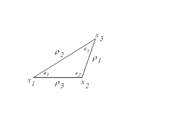
Figure 6: The triangle spanned by $x_{1},x_{2},x_{3}$.

We also denote the spin associated with a field $\phi_{a}$ by $\hat{a}\in\frac{1}{2}{\mathbb{N}}$. Then the associativity condition (5.61) is equivalent to the following condition:

$$\sum_{b}\sum_{j_{1},j_{2},j_{5}}\left\{\begin{matrix}j_{6}&j_{2}&\hat{a}_{4}\\ j_{7}&j_{5}&j_{1}\end{matrix}\right\}\left\{\begin{matrix}j_{3}&j_{5}&\hat{b}\\ j_{1}&\hat{a}_{3}&j_{6}\end{matrix}\right\}\,{\rm P}_{j_{1}}(\cos\theta_{2})$$ (7.131)

$$\times f_{a_{1}a_{2}}^{b}\Big{(}\rho_{3};[j_{3}j_{1}]\Big{)}f_{ba_{3}}^{a_{4}}\Big{(}\rho_{1};[j_{5}j_{2}]\Big{)}=$$

$$\sum_{b}\sum_{j_{1},j_{2},j_{4},j_{5}}\left\{\begin{matrix}j_{6}&j_{2}&\hat{a}_{4}\\ j_{7}&j_{5}&j_{1}\end{matrix}\right\}\left\{\begin{matrix}j_{4}&j_{5}&\hat{a}_{5}\\ j_{1}&\hat{a}_{2}&j_{6}\end{matrix}\right\}\left\{\begin{matrix}\hat{a}_{1}&j_{6}&j_{4}\\ \hat{a}_{3}&\hat{a}_{2}&j_{5}\end{matrix}\right\}\,{\rm P}_{j_{1}}(\cos\theta_{3})$$

$$\times f_{a_{1}a_{3}}^{b}\Big{(}\rho_{2};[j_{4}j_{1}]\Big{)}f_{a_{2}b}^{a_{4}}\Big{(}\rho_{1};[j_{5}j_{2}]\Big{)}\,,$$

in the domain $\rho_{3}<\rho_{1}<\rho_{2}$. Here, the expressions in brackets denote the well-known $6j$-symbols for $SU(2)$,

$$\left\{\begin{matrix}j_{1}&j_{2}&j_{3}\\ j_{4}&j_{5}&j_{6}\end{matrix}\right\}=\left\{\begin{matrix}j_{3}\\ j_{1}\,\,\,\,j_{2}\end{matrix}\right\}\left\{\begin{matrix}j_{4}\\ j_{3}\,\,\,\,j_{5}\end{matrix}\right\}\left\{\begin{matrix}j_{5}\,\,\,\,j_{2}\\ j_{6}\end{matrix}\right\}\left\{\begin{matrix}j_{6}\,\,\,\,j_{1}\\ j_{4}\end{matrix}\right\}\,.$$ (7.132)

The expressions ${\rm P}_{j}(z)={}_{2}F_{1}(-j,j+1,1;(1-z)/2)$ are the Legendre polynomials. A similar form of the associativity condition can be obtained for arbitrary dimensions $D\geq 3$, the only essential difference being that we now encounter the $6j$-symbols for the spin groups of $SO(D)$ for general $D$. The case $D=2$ is an exceptional case and the corresponding expression is much simpler, owing to the fact that the representation theory $SO(2)$ and its covering ${\mathbb{R}}$ is much simpler.

If we let $|a|$ be the dimension of the field $\phi_{a}$, then the scaling axiom for the OPE-coefficients implies the relation

$$f_{ab}^{c}(r)=O(r^{|c|-|a|-|b|})\,.$$ (7.133)

In the case of the free quantum field theory in 3 dimensions defined by the Lagrangian $L=\frac{1}{2}(\partial\varphi)^{2}$, the coefficients are in fact monomials and are given by $f_{ab}^{c}(r)=\zeta_{ab}^{c}r^{|c|-|a|-|b|}$ for some complex constants $\zeta^{c}_{ab}$, see section 9 for details. Furthermore, one can show that [16], for the coefficients of the perturbatively defined theory with Lagrangian $L=\frac{1}{2}(\partial\varphi)^{2}-\frac{1}{6}\lambda\varphi^{6}$ and dimensionless $\lambda$, the coefficients take the form

$$f_{ab}^{c}(r)=p_{ab}^{c}(\log r,\lambda)r^{|c|-|a|-|b|}\,,$$ (7.134)

with $p_{ab}^{c}$ a polynomial in two variables whose degree is $n$ in $\lambda$ if we compute the coefficients to $n$-th order in perturbation theory, and whose degree in $\log r$ is no more than $n$ at $n$-th order. The associativity condition (7.131) is a quadratic constraint for these polynomials $p_{ab}^{c}$ at each arbitrary but fixed order in perturbation theory.

If there are dimensionful parameters in the lagrangian, those would effectively be treated as other perturbations in our framework. For example, for the Lagrangian $L=\frac{1}{2}(\partial\varphi)^{2}+\frac{1}{2}m^{2}\varphi^{2}+\frac{1}{6}\lambda\varphi^{6}$, the coefficients take the form

$$f_{ab}^{c}(r)=p_{ab}^{c}(r,\log r,m^{2},\lambda)r^{|c|-|a|-|b|}\,,$$ (7.135)

where $p_{ab}^{c}$ is again a polynomial in all four variables at $n$-th perturbation order in $m^{2}$ and $\lambda$. Each term in this polynomial containing a power $m^{2k}$ contains exactly a power of $r^{2k}$ so as to make each term ”dimensionless” (with the logarithms and $\lambda$ not counting as having a dimension).

8 The fundamental left (vertex algebra) representation

In the previous sections, we have elaborated on our definition of quantum field theory in terms of consistency conditions. Our formulation involved only the OPE coefficients such as $C_{ab}^{c}$. To motivate our constructions, we sometimes wrote formal relations like

$$\text{``$\phi_{a}(x_{1})\phi_{b}(x_{2})=\sum_{c}C_{ab}^{c}(x_{1},x_{2})\,\phi_{c}(x_{2})$''}\quad.$$ (8.136)

But these relations were only heuristic, in the sense that none of our proposed properties of the OPE coefficients relied on the existence or properties of the hypothetical operators $\phi_{a}$, which were only ”dummy variables”. As we have emphasized, our approach is similar to the standard viewpoint taken in algebra that an abstract algebra ${\bf A}$ is entirely defined in terms of its product—i.e., a linear map $m:{\bf A}\otimes{\bf A}\to{\bf A}$ subject to the associativity condition. But, as in our case, the algebra elements need not be represented a priori by linear operators on a vector space. Representations in the context of an algebra are an additional structure defined as linear maps $\pi:{\bf A}\to{\rm End}(H)$ from the algebra to the linear operators on a vector space $H$, subject to the condition $\pi[m(A,B)]=\pi(A)\pi(B)$. It is natural to ask whether there is a construction similar to a representation also in our context. We shall show in this section that there is indeed a certain ”canonical” construction, which has some features in common with an algebra representation, and which will be useful in the next section. We will refer to this construction as the ”fundamental left-” or ”vertex algebra representation”.

Definition 8.1.

Let $|v\rangle\in V$ be an arbitrary vector. We define a corresponding vertex operator ${\cal Y}(x,v):V\to V$ by the formula

$${\cal Y}(x,v)|w\rangle={\cal C}(x,0)(|v\rangle\otimes|w\rangle)\,,$$ (8.137)

for all $x\neq 0$. In a basis $\{|v_{a}\rangle\}$, the matrix representing the vertex operator is hence given by

$$[{\cal Y}(x,v_{a})]_{b}^{c}:=C_{ab}^{c}(x,0)\,\,\,\,\,.$$ (8.138)

This is our fundamental left- or vertex algebra representation.

Using the consistency condition (5.61), one can immediately show that

$${\cal Y}(x,v_{a}){\cal Y}(y,v_{b})=\sum_{c}C_{ab}^{c}(x,y)\,{\cal Y}(y,v_{c})\,,$$ (8.139)

for $0<|x-y|<|y|<|x|$, or equivalently that

$${\cal Y}(x,v_{a}){\cal Y}(y,v_{b})={\cal Y}(y,{\cal Y}(x-y,v_{a})v_{b})\,.$$ (8.140)

Thus, by eq. (8.139), the vertex operators operators ${\cal Y}(x,v_{a}):V\to V$ satisfy the operator product expansion. The fact that the OPE coefficients in this expansion are precisely the matrix elements of the vertex operators themselves is expressed in the second relation (8.140). This quadratic relation is the key axiom in the theory of vertex operator algebras, see [2, 3, 4, 5]. Because of eq. (8.139), we may formally view the vertex operators as forming a ”representation” of the heuristic field operators, i.e., formally ”$\pi(\phi_{a}(x))={\cal Y}(x,v_{a})$” is a ”representation” of the ”algebra” defined by the OPE coefficients. This ”representation” is in some sense analogous to the GNS-representation (see e.g. [1]) for $C^{*}$-algebras. However, we emphasize that in our case, $V$ is not in a natural way a Hilbert space, and should not be confused with the physical Hilbert space obtained via the Osterwalder-Schrader reconstruction theorem, see our remarks in section 3. We will further develop the analogy of our approach to the theory of vertex operator algebras in a forthcoming paper [38].

9 Example: The free field

Let us now explain our approach to quantum field theory in a simple example, namely that of a free hermitian bosonic scalar field in $D$ dimensions classically described by the field equation

$$\square\varphi=0,$$

with $\square=\delta^{\mu\nu}\partial_{\mu}\partial_{\nu}$. The aim is to present explicitly the OPE coefficients ${\cal C}(x_{1},x_{2})$ for this model. This section is joint work with H. Olbermann and details will appear elsewhere. We begin by describing the space $V$ of fields in our case, assuming $D>2$ for simplicity. The case $D=2$ can be treated analogously, with only minor modifications.

Definition 9.1.

$V$ is the defined to be the commutative, unital, ${\mathbb{C}}$-module generated as a module (i.e., under addition, multiplication and scalar multiplication) by formal expressions of the form $\partial_{\{\mu_{1}}\dots\partial_{\mu_{N}\}}\varphi$, and unit ${\bf 1}$, where $\mu_{i}=1,\dots,D$ and a curly bracket denotes the totally symmetric, trace-free part, i.e. by definition,

$$\delta^{\mu_{i}\mu_{j}}\,\partial_{\{\mu_{1}}\dots\partial_{\mu_{N}\}}\varphi=0\,.$$ (9.141)

The trace free condition has been imposed because any trace would give rise to an expression containing $\square\varphi$, which we want to vanish in order to satisfy the field equation on the level of $V$. A basis of $V$ as a ${\mathbb{C}}$-vector space can e.g. be given as follows. First, let us choose a basis of totally symmetric, trace-free, rank-$l$ tensors in ${\mathbb{R}}^{D}$ for any $l\geq 0$. For a given $l\geq 0$, this space has dimension $N(l,D)$, where

$$N(l,D)=\begin{cases}1&\text{for $l=0$}\\ \frac{(2l+D-2)(l+D-3)!}{(D-2)!l!}&\text{for $l>0$.}\end{cases}$$ (9.142)

We denote the basis elements by $t_{l,m},m=1,\dots,N(l,D)$, and we assume for convenience that they are orthonormal with respect to the natural hermitian inner product on $({\mathbb{R}}^{D})^{\otimes l}$ coming from the Euclidean metric on ${\mathbb{R}}^{D}$, i.e. $\bar{t}_{l^{\prime},m^{\prime}}\cdot t_{l,m}=\delta_{ll^{\prime}}\delta_{mm^{\prime}}$. A basis of $V$ is then given by ${\bf 1}$, together with the elements

$$|v_{a}\rangle=\prod_{l,m}(a_{l,m}!)^{-1/2}\left(c_{l}^{-1/2}\,t_{l,m}\cdot\partial^{l}\varphi\right)^{a_{l,m}}\,\quad\,,$$ (9.143)

where $a=\{a_{l,m}\mid l\geq 0,0<m\leq N(l,D)\}$ is a multi-index of non-negative integers, only finitely many of which are non-zero. For later convenience, we also set

$$c_{l}=\frac{2^{l}\,\Gamma(l+1)\Gamma(l+D/2-1)}{\Gamma(D/2-1)}\,.$$ (9.144)

The canonical dimension of $|v_{a}\rangle$ is defined as

$$|a|=\sum_{l,m}a_{l,m}[(D-2)/2+l]\,.$$ (9.145)

It is possible to formally view $V$ as a ”Fock-space”, with $a_{l,m}$ the ”occupation numbers” of the ”mode” labeled by $l,m$. On this Fock-space, one can then define creation and annihilation operators ${\mathbf{b}}_{l,m},{\mathbf{b}}_{l,m}^{+}:V\to V$ as usual. These are defined explicitly by

$${\mathbf{b}}_{l,m}|v_{a}\rangle := (a_{l,m})^{1/2}\,|v_{a-e_{l,m}}\rangle$$ (9.146)

$${\mathbf{b}}_{l,m}^{+}|v_{a}\rangle := (a_{l,m}+1)^{1/2}\,|v_{a+e_{l,m}}\rangle$$ (9.147)

where $e_{l,m}$ is the multiindex with a unit entry at position $l,m$ and zeros elsewhere. They satisfy the standard commutation relations

$$\left[{\mathbf{b}}_{l,m},{\mathbf{b}}_{l^{\prime},m^{\prime}}^{+}\right]=\delta_{ll^{\prime}}\delta_{mm^{\prime}}\,\,id\,,\quad\left[{\mathbf{b}}_{l,m}^{+},{\mathbf{b}}_{l^{\prime},m^{\prime}}^{+}\right]=\left[{\mathbf{b}}_{l,m},{\mathbf{b}}_{l^{\prime},m^{\prime}}\right]=0$$ (9.148)

where $id$ is the identity operator on $V$. The “vacuum” vector $|0\rangle$ in this Fock space by definition corresponds to the identity operator ${\bf 1}\in V$.

To present the OPE coefficients of the model, it is further convenient to introduce spherical harmonics in $D$ dimensions. The most straightforward way to do this is as follows. Let $l\in{\mathbb{N}}_{0}$, and let $h_{l}(x)\in{\mathbb{C}}[x]$ be a harmonic polynomial on ${\mathbb{R}}^{D}$ that is homogeneous of degree $l$, meaning that $\square h_{l}(x)=0$, and that $h(\lambda x)=\lambda^{l}h_{l}(x)$ for all $\lambda\in{\mathbb{R}}_{+}$. It is not difficult to see that the vector space spanned by such polynomials is of dimension $N(l,D)$. We let $h_{l,m}(x),0<m\leq N(l,D)$ be a basis of this vector space and we define the (scalar) spherical harmonics $Y_{l,m}:S^{D-1}\to{\mathbb{C}}$ to be the restriction of the corresponding harmonic polynomials to the $(D-1)$-dimensional sphere. We normalize the spherical harmonics to turn them into an orthonormal basis on the sphere, in the natural $L^{2}$-inner product. The spherical harmonics are closely related to the trace free symmetric tensors $t_{l,m}$ in $({\mathbb{R}}^{D})^{\otimes l}$ that were introduced above. In fact, we may choose

$$Y_{l,m}(\hat{x})=k_{l}\,\bar{t}_{l,m}\cdot\hat{x}^{\otimes l}\,,$$ (9.149)

for some normalization constant $k_{l}$. With this notation in place, we now explicitly present the OPE coefficients ${\cal C}(x_{1},x_{2})$ for this model. For this, it is sufficient to present the vertex operators (left-representatives) ${\cal Y}(x,v_{a}):V\to V$ for all $|v_{a}\rangle\in V$, since the matrix elements $[{\cal Y}(x,v_{a})]_{b}^{c}=C_{ab}^{c}(x,0)$ are by definition just the OPE coefficient components, see sec. 8. First, we give the formula for ${\cal Y}(x,\varphi)$ corresponding to the basic field $\varphi\in V$. This is defined by

$${\cal Y}(x,\varphi)=\sqrt{{\rm vol}(S^{D-1})}\,\sum_{l=0}^{\infty}\,\sum_{m=1}^{N(l,D)}\sqrt{\frac{D-2}{2l+D-2}}\times\\ \Big{[}r^{l}Y_{l,m}(\hat{x})\,{\mathbf{b}}_{l,m}^{+}+r^{-l-D+2}\overline{Y_{l,m}(\hat{x})}\,{\mathbf{b}}_{l,m}\Big{]}\,.$$ (9.150)

We will ”derive” this formula from the standard quantum field theory formalism in a future paper [38]. Accidentally, this has precisely the familiar form for a free field operator, with an ”emissive” and an ”absorptive” piece, which should not come as a surprise, since ${\cal Y}(x,\varphi)$ is in a sense the ”representative” of the (formal) field operator $\varphi(x)$ on $V$. Actually, if we furthermore write $r={\rm e}^{t}$, then this is precisely the formula for a free field operator on the manifold ${\mathbb{R}}\times S^{D-1}$ with ”time” $t$ formally imaginary. We will pursue this analogy elsewhere.

For a general element in $V$, we now give a corresponding formula for the vertex operator. It is defined by ${\cal Y}(x,{\bf 1})=id$ for the identity element, and by

$${\cal Y}\Big{(}x,\prod_{i}\partial^{l_{i}}\varphi\Big{)}=\,\,:\prod_{i}\partial^{l_{i}}{\cal Y}\Big{(}x,\varphi\Big{)}:\,\,\,.$$ (9.151)

for a general field monomial. Here, the following notation is used. The double dots $:\dots:$ mean ”normal ordering”, i.e., all creation operators are to the right of all annihilation operators. Again, one can derive this formula using the standard quantum field theory formalism. The OPE coefficients for the free field are consequently given by $C_{ab}^{c}(x_{1},x_{2}):=[{\cal Y}(x_{1}-x_{2},v_{a})]_{b}^{c}=\langle v^{c}|{\cal Y}(x_{1}-x_{2},v_{a})|v_{b}\rangle$ or more explicitly by

$$C_{ab}^{c}(x_{1},x_{2}):=\Big{\langle}0\Big{|}\prod_{l,m}({\mathbf{b}}_{l,m})^{c_{l,m}}\,{\cal Y}(x_{1}-x_{2},v_{a})\,\prod_{l,m}({\mathbf{b}}_{l,m}^{+})^{b_{l,m}}\Big{|}0\Big{\rangle}\,.$$ (9.152)

We now state that the so-defined OPE-coefficients satisfy our consistency condition:

Theorem 2.

Let ${\cal Y}(x,v):V\to V$ be defined for our model by formula (9.151), and let the OPE-coefficients $C_{ab}^{c}(x_{1},x_{2})$ be defined by eq. (9.152). Then the OPE coefficients satisfy the consistency condition (5.61). Equivalently, the vertex algebra condition (8.140) holds for the free field vertex operators ${\cal Y}(x,v_{a})$.

Proof: The proof of this theorem is essentially a longish but straightforward computation, using various standard identities for the $D$-dimensional spherical harmonics. We will give a complete proof in [38].

10 Interacting fields

In the previous section, we have presented the (2-point) OPE coefficients in the example of a free quantum field associated with the classical equation $\square\varphi=0$. It is clearly of interest to know what would be the corresponding coefficients for a field associated with a non-linear equation such as

$$\square\varphi=\lambda\varphi^{p}$$ (10.153)

where $p$ is some non-negative integer. As has been appreciated for a long time, the construction of a quantum field theory (and hence in particular of the OPE) associated with such an equation is extremely difficult, and has only been accomplished so far for certain values of $p,D$ where the theory has a particularly simple behavior. However, one can treat $\lambda$ as a formal perturbation parameter, and try to construct the OPE coefficients in the sense of formal power series in $\lambda$ as we have outlined in general terms in section 6. Here we would like to outline how a field equation can help to actually determine the formal power series in the theory described by a field equation of the above type. Some of the ideas in this section go back, in preliminary form, to discussions with N. Nikolov, and also to joint work with H. Olbermann, which will be published in [38].

As we have seen in section 8, the 2-point OPE coefficients ${\cal C}(x_{1},x_{2})$ contain the same information as the corresponding vertex operators ${\cal Y}(x,v)$. In perturbation theory, they are given by formal power series

$${\cal Y}(x,v)=\sum_{i=0}^{\infty}{\cal Y}_{i}(x,v)\,\lambda^{i}\,,$$ (10.154)

where each ${\cal Y}_{i}(x,v)$ is a linear map $V\to V$, and where ${\cal Y}_{0}(x,v)$ is given by the free field vertex operator defined in the previous section 9. As discussed in subsection 2.4, we expect that the field equation implies:

$${\cal Y}_{i}(x,\varphi)=\square^{-1}{\cal Y}_{i-1}(x,\varphi^{p})\,.$$ (10.155)

More precisely, in this section we assume the existence of ${\cal Y}_{i}$ satisfying this equation, and we also assume that the consistency condition (8.140) is satisfied order-by-order; in vertex operator notation

$$\sum_{j=0}^{i}{\cal Y}_{j}(y,v_{a}){\cal Y}_{i-j}(x,v_{b})=\sum_{j=0}^{i}{\cal Y}_{i-j}\Big{(}x,{\cal Y}_{j}(y-x,v_{a})v_{b}\Big{)}\,.$$ (10.156)

As we will now show, these assumptions will allow us to inductively determine the actual form of the vertex operators order by order in $i$. But before we do this, we must explain a point related to the choice of $V$ in for our interacting theory. Recall that, in the underlying free theory with $\lambda=0$, $V$ was spanned by formal monomials in $\varphi$ and its derivatives $\partial_{\{\mu_{1}}\dots\partial_{\mu_{N}\}}\varphi$, where he curly brackets denote the trace-free part of a tensor. In the free theory, we considered the trace free part only, since any trace gives rise to a factor of $\square\varphi$ in such a monomial, $v$, and the corresponding vertex operator ${\cal Y}_{0}(x,v)$ then vanishes (essentially by definition). However, for the interacting theory, we must be more careful and allow also traces, i.e., we also consider vertex operators whose arguments are formal monomials in $\varphi$ and its derivatives $\partial_{\mu_{1}}\dots\partial_{\mu_{N}}\varphi$. This enlarged space of objects, $\widehat{V}$, is a commutative unital differential module (with derivations $\partial_{\mu},\mu=1,\dots,D$ acting in the usual way), and the vertex operators ${\cal Y}_{i}(x,v)$ should now be considered as linear maps $\widehat{V}\owns v\mapsto{\cal Y}_{i}(x,v)\in{\rm End}(\widehat{V})$. We then also assume to have a relation

$$\partial_{\mu}\,{\cal Y}_{i}(x,v)={\cal Y}_{i}(x,\partial_{\mu}v)\quad,\quad\mu=1,\dots,D\,,$$ (10.157)

where the symbol $\partial_{\mu}$ denotes a genuine partial $x$-derivative on the left side, while it is the derivation on the differential module $\widehat{V}$ on the right side. For details, we refer to [38]. To lighten the notation, we will drop the caret on $\widehat{V}$ again for the remaining part of the section.

To make sense of eq. (10.155), we first of all need to define the inverse of the Laplace operator. We rewrite it in $D$-dimensional polar coordinates, and we furthermore assume that we can expand each vertex operator in spherical harmonics and coefficients in the ring ${\mathbb{C}}[r,1/r,\log r]\otimes{\rm End}(V)$. Then the vertex operators schematically take the form

$${\cal Y}_{i}(x,v)=\sum A_{i,l,m,j,k}(v)r^{k}(\log r)^{j}Y_{l,m}(\hat{x})\,,$$ (10.158)

with $A_{i,l,m,j,k}(v)\in{\rm End}(V)$. We define the action of the inverse Laplacian on such expressions by putting

$$\square^{-1}[r^{k}(\log r)^{j}Y_{l,m}(\hat{x})]:=j!Y_{l,m}(\hat{x})\times$$

$$\times\begin{cases}(-1)^{j+1}r^{l}\sum_{i=0}^{j+1}\frac{(-1)^{i}\log^{i}r}{i!(2l+D-2)^{j-i+2}}&\text{if $k=l-2$}\\ -r^{-l-D+2}\sum_{i=0}^{j+1}\frac{\log^{i}r}{i!(2l+D-2)^{j-i+2}}&\text{if $k=-l-D$}\\ r^{k+2}\sum_{i=0}^{j}\sum_{n=0}^{i}\frac{(-1)^{i-n}\log^{j-i}r}{(j-i)!(l-k-2)^{n+1}(l+k+D)^{i-n+1}}&\text{otherwise.}\end{cases}$$ (10.159)

This is a left inverse for the Laplacian. Any other left inverse can differ from this one only by terms in the kernel of $\square$, i.e. a harmonic polynomial of $x$ with values in ${\rm End}(V)$.

Let us now assume inductively that we have constructed all the vertex operators ${\cal Y}_{j}(x,v)$ up to order $j=i-1$. The vertex operator ${\cal Y}_{i}(x,\varphi)$ is then given by eq. (10.155). Next, we would like to determine all other vertex operators ${\cal Y}_{i}(x,v)$, where $|v\rangle\in V$ is a general element. For this, we perform, at fixed $i$, an induction in the dimension $\Delta(v)$. Thus, let us assume that we have succeeded in constructing all vertex operators up to dimension $d$, and let us assume for the sake of concreteness that we are in $D=4$, so that $\Delta(\varphi)=1$. We may hence assume that $d\geq 2$. We may write a general field of dimension $d+1$ as a linear combination of fields of the form $v=w\partial^{l}\varphi$, or of the form $v=\partial^{l+1}w$. In both cases, $w$ has dimension $d-l$, and so ${\cal Y}_{j}(x,w)$ is inductively known for $0\leq j\leq i$. In the second case, we must have ${\cal Y}_{i}(x,v)=\partial^{l+1}{\cal Y}_{i}(x,w)$. In the first case, the consistency condition gives

$$\sum_{j=0}^{i}{\cal Y}_{j}\Big{(}y,\partial^{l}\varphi\Big{)}{\cal Y}_{i-j}\Big{(}x,w\Big{)}=\sum_{j=0}^{i}{\cal Y}_{i-j}\Big{(}x,{\cal Y}_{j}(y-x,\partial^{l}\varphi)w\Big{)}\,.$$ (10.160)

By the inductive hypothesis, all operators on the left side of the equation are already known. Now we investigate which operators are not already known on the right side. Evidently, if $j\neq 0$, then all terms in the corresponding expression are known. If $j=0$, we look at the terms that survive in the limit $y\to x$. Using the definition of the zeroth order vertex operators (free theory), we see that

$${\cal Y}_{0}(y-x,\partial^{l}\varphi)w=w\partial^{l}\varphi+\dots,$$ (10.161)

where the dots stand for the following terms: (a) terms that vanish as $|x-y|\to 0$ and (b) a finite Laurent series in $1/|x-y|$ with coefficients that are vectors of dimension $\leq d$. Let $P_{d}^{j}:V\to V$ denote the map which is the identity for $j\neq 0$, which is the projector onto the subspace of vectors of dimension $\leq d$ for $j=0$. Then we can write:

$${\cal Y}_{i}(x,v)=\lim_{y\to x}\Bigg{[}\sum_{j=0}^{i}{\cal Y}_{j}\Big{(}y,\partial^{l}\varphi\Big{)}{\cal Y}_{i-j}\Big{(}x,w\Big{)}\\ -\sum_{j=0}^{i}{\cal Y}_{i-j}\Big{(}x,P_{d}^{j}\circ{\cal Y}_{j}(y-x,\partial^{l}\varphi)w\Big{)}\Bigg{]}\,.$$ (10.162)

Now all the terms on the right side are known inductively. We can hence determine all vertex operators at order $i$, and hence to arbitrary orders. This shows how we may construct inductively the terms in the perturbation series starting from those of the free theory.

11 Conclusions and outlook

In this paper, we have suggested a new approach to general, non-conformal, quantum field theories in terms of consistency conditions. These consistency conditions are formulated in terms of the operator product expansion (OPE). We showed that these conditions are quite powerful. For example, they can be used to characterize the possible perturbations of the quantum field theory, and give rise to an efficient algorithm for explicitly computing these coefficients.

This paper is just the beginning of a longer programme. In the future, we would like to extend the ideas of the paper. In particular, it would be interesting to consider the following issues:

• Generalization of our approach to curved space-time;

• Convergence/Borel summability of the perturbation series;

• Explicit perturbative calculations;

• Incorporation of the renormalization group into our approach;

• (Super-)conformal quantum field theories;

• Perturbations of 2-dimensional conformal quantum field theories.

We intend to study these topics in future publications.




Acknowledgements: I would like to thank N. Nikolov for extensive discussions on various topics in this paper. I would also like to thank K.-H. Rehren and R. M. Wald for discussions. I would especially like to thank C. Brouder for his careful reading of the manuscript, and in particular for pointing out several sign errors in the first version.

References

- [1] R. Haag: ”Local Quantum Physics”, Springer Verlag (1994)
- [2] R. E. Borcherds, “Vertex Algebras, Kac-Moody Algebras, And The Monster,” Proc. Nat. Acad. Sci. 83, 3068 (1986).
- [3] V. Kac, “Vertex algebras for beginners,” Providence, USA: AMS (1996) 141 p. (University lectures series. 10)
-
[4]
I. Frenkel, J. Lepowsky and A. Meurman,
“Vertex operator algebras and the Monster,”
http://www.slac.stanford.edu/spires/find/hep/www?irn=2107686
Academic Press, Boston (1988) - [5] N. M. Nikolov, “Vertex algebras in higher dimensions and global conformally invariant quantum field theory,” Commun. Math. Phys. 253, 283 (2004) [arXiv:hep-th/0307235].
- [6] M. R. Gaberdiel and P. Goddard, “Axiomatic conformal field theory,” Commun. Math. Phys. 209, 549 (2000) [arXiv:hep-th/9810019].
- [7] N. M. Nikolov, K. H. Rehren and I. T. Todorov, “Partial wave expansion and Wightman positivity in conformal field theory,” Nucl. Phys. B 722, 266 (2005) [arXiv:hep-th/0504146].
- [8] N. M. Nikolov, K. H. Rehren and I. Todorov, “Harmonic bilocal fields generated by globally conformal invariant scalar fields,” arXiv:0704.1960 [hep-th].
- [9] S. Hollands and R. M. Wald, “Local Wick polynomials and time ordered products of quantum fields in curved spacetime,” Commun. Math. Phys. 223, 289 (2001) [arXiv:gr-qc/0103074].
- [10] S. Hollands and R. M. Wald, “Existence of local covariant time ordered products of quantum fields in curved spacetime,” Commun. Math. Phys. 231, 309 (2002) [arXiv:gr-qc/0111108].
- [11] R. Brunetti and K. Fredenhagen, “Microlocal analysis and interacting quantum field theories: Renormalization on physical backgrounds,” Commun. Math. Phys. 208, 623 (2000) [arXiv:math-ph/9903028].
- [12] R. Brunetti, K. Fredenhagen and R. Verch, “The generally covariant locality principle: A new paradigm for local quantum physics,” Commun. Math. Phys. 237, 31 (2003) [arXiv:math-ph/0112041].
- [13] K. G. Wilson, “Nonlagrangian models of current algebra,” Phys. Rev. 179, 1499 (1969).
- [14] K. G. Wilson and W. Zimmermann, “Operator Product Expansions And Composite Field Operators In The General Framework Of Quantum Field Theory,” Commun. Math. Phys. 24, 87 (1972).
- [15] W. Zimmermann, “Normal products and the short distance expansion in the perturbation theory of renormalizable interactions,” Annals Phys. 77, 570 (1973) [Lect. Notes Phys. 558, 278 (2000)].
- [16] S. Hollands, “The operator product expansion for perturbative quantum field theory in curved spacetime,” Commun. Math. Phys. 273, 1 (2007) [arXiv:gr-qc/0605072].
- [17] S. Hollands and R.M. Wald: ”Axiomatic quantum field theory in curved spacetime”, to appear.
- [18] A. A. Migdal, “4-dimensional soluble models of conformal quantum field theory,” 1972
- [19] A. M. Polyakov, “Non-Hamiltonian approach to quantum field theory at small distances,” 1972
- [20] G. Mack: “Osterwalder-Schrader Positivity in Conformal invariant quantum field theory,” Trends in Elem. Part. Theory, LNP 37, Rollnick, Dietz (eds.), Springer 1975
- [21] G. Mack: “Group theoretical approach to conformal field theories,” Karpasz Winter school proceedings 1973
- [22] I. T. Todorov, “Conformal expansions for Euclidean Green’s functions,” 1974
- [23] O. Steinmann, “Perturbation theory of Wightman functions,” Commun. Math. Phys. 152 (1993) 627.
- [24] N. Nikolov: Unpublished notes, Göttingen, May 2005
- [25] K. Osterwalder and R. Schrader, “Axioms for Euclidean Green’s functions,” Commun. Math. Phys. 31 (1973) 83.
- [26] K. Osterwalder and R. Schrader, “Axioms For Euclidean Green’s Functions. 2,” Commun. Math. Phys. 42, 281 (1975).
- [27] See e.g. sec. VII.2 in: S. MacLane: ”Categories for the working mathematician” Graduate Texts in Mathematics, vol. 5, Springer Verlag (1995)
- [28] S. MacLane: ”Homology” Grundlehren der mathematischen Wissenschaften ; Vol. 114, Springer (1995)
- [29] D. Happel: ”Hochschild Cohomology of Finite-dimensional Algebras.” Number 1404 in Lecture Notes in Mathematics, Springer-Verlag (1989)
- [30] A. Connes: ”Non-Commutative Differential Geometry,” Publ. Math. IHES 62 (1985).
- [31] L. D. Faddeev and V. N. Popov, “Feynman diagrams for the Yang-Mills field,” Phys. Lett. B 25, 29 (1967).
- [32] M. Henneaux and C. Teitelboim, “BRST cohomology in classical mechanics,” Commun. Math. Phys. 115, 213 (1988).
- [33] C. Becchi, A. Rouet and R. Stora, “Renormalization Of Gauge Theories,” Annals Phys. 98, 287 (1976).
-
[34]
R. F. Streater and A. S. Wightman,
“PCT, spin and statistics, and all that,”
http://www.slac.stanford.edu/spires/find/hep/www?irn=2423855
Addison-Wesley (1989) (Advanced book classics) - [35] S. Hollands, “A general PCT theorem for the operator product expansion in curved spacetime,” Commun. Math. Phys. 244, 209 (2004) [arXiv:gr-qc/0212028].
- [36] M. Gerstenhaber: ”On the deformation of rings and algebras” Ann. Math. 79 59–103 (1964)
- [37] G. Barnich, F. Brandt and M. Henneaux, “Local BRST cohomology in gauge theories,” Phys. Rept. 338, 439 (2000) [arXiv:hep-th/0002245].
- [38] S. Hollands, H. Olbermann: In preparation.