Multi-particle collision dynamics modeling of viscoelastic fluids

Abstract

In order to investigate the rheological properties of viscoelastic fluids by mesoscopic hydrodynamics methods, we develop a multi-particle collision dynamics (MPC) model for a fluid of harmonic dumbbells. The algorithm consists of alternating streaming and collision steps. The advantage of the harmonic interactions is that the integration of the equations of motion in the streaming step can be performed analytically. Therefore, the algorithm is computationally as efficient as the original MPC algorithm for Newtonian fluids. The collision step is the same as in the original MPC method. All particles are confined between two solid walls moving oppositely, so that both steady and oscillatory shear flows can be investigated. Attractive wall potentials are applied to obtain a nearly uniform density everywhere in the simulation box. We find that both in steady and oscillatory shear flow, a boundary layer develops near the wall, with a higher velocity gradient than in the bulk. The thickness of this layer is proportional to the average dumbbell size. We determine the zero-shear viscosities as a function of the spring constant of the dumbbells and the mean free path. For very high shear rates, a very weak “shear thickening” behavior is observed. Moreover, storage and loss moduli are calculated in oscillatory shear, which show that the viscoelastic properties at low and moderate frequencies are consistent with a Maxwell fluid behavior. We compare our results with a kinetic theory of dumbbells in solution, and generally find good agreement.

I Introduction

It is the characteristic feature of soft matter systems that a macromolecular component of nano- to micrometer size is dispersed in a solvent of much smaller molecules. The mesoscopic length scale of the dispersed component implies that crystalline phases have a very small shear modulus – which roughly scales like the inverse of the third power of the structural length scale – and that both crystalline and fluid phases are characterized by long structural relaxation times. Soft matter systems have therefore interesting dynamical properties, because the time scale of an external perturbation can easily become comparable with the intrinsic relaxation time of the dispersed macromolecules.

One of the unique properties of soft matter is its viscoelastic behaviorLarson (1999). Due to the long structural relaxation time, the internal degrees of freedom cannot relax sufficiently fast in an oscillatory shear flow, so that there is some elastic restoring force which pushes the system back to its previous state. A very well studied example of viscoelastic fluids are polymer solutions and polymer meltsFerry (1980); Doi and Edwards (1986); Larson (1999). In the case of polymer melts, the characteristic time scale is given by the reptation time, i.e. by the time it takes a chain to slide by its contour length along the tube formed by other polymer chainsDoi and Edwards (1986).

In order to bridge the length- and time-scale gap between the solvent and macromolecular or colloidal scales, several mesoscopic simulation techniques – such as the lattice-Boltzmann method, dissipative-particle dynamics (DPD), and multi-particle collision dynamics (MPC) – have been suggested in recent years, and are in the process of being developed further. The idea of all these methods is to strongly simplify the microscopic dynamics in order to gain computational efficiency, but at the same time to exactly satisfy the conservation laws of mass, momentum and energy, so that hydrodynamic behavior emerges naturally on larger length scales.

We will focus here on the multi-particle collision dynamics (MPC) techniqueMalevanets and Kapral (1999, 2000); Lamura et al. (2001), also called stochastic rotation dynamicsIhle and Kroll (2001) (SRD), originally developed for Newtonian fluids. This particle-based hydrodynamics method consists of alternating streaming and collision steps. In the streaming step, point particles move ballistically. In the collision step, particles are sorted into the cells of a simple cubic (or square) lattice. All particles in a cell collide by a rotation of their velocities relative to the center-of-mass velocity around a random axisMalevanets and Kapral (1999). A random shift of the cell lattice is performed before each collision step in order to restore Galilean invarianceIhle and Kroll (2001). This method has been applied very successfully to study the hydrodynamic behavior of many complex fluids, such as polymer solutions in equilibriumMussawisade et al. (2005); Lee and Kapral (2006) and flowWebster and Yeomans (2005); Ryder and Yeomans (2006); Ripoll et al. (2006), colloidal dispersionsPadding and Louis (2004); Hecht et al. (2005), vesicle suspensionsNoguchi and Gompper (2004, 2005), and reactive fluidsTucci and Kapral (2004); Echeveria et al. (2007).

The viscoelastic behavior of polymer solutions leads to many unusual flow phenomena, such as shear-induced phase separationHelfand and Fredrickson (1989); Onuki (1989); Milner (1993), viscoelastic phase separationTanaka (2000), and elastic turbulenceGroisman and Steinberg (2000). A coarse-grained description of viscoelastic fluids is necessary in order to obtain a detailed understanding of the role of elastic forces in such flow instabilities.

However, there is a second level of complexity in soft matter system, in which a colloidal component is dispersed in a solvent, which is itself a complex fluid. Examples are spherical or rod-like colloids dispersed in polymer solutions or melts, which are exposed to a shear flowLyon et al. (2001); Suen et al. (2002); Hwang et al. (2004); Scirocco et al. (2004); Vermant and Solomon (2005). Shear flow can induce particle aggregation and alignment in these systems. This is important, for example, in the processing of nanocompositesVermant and Solomon (2005).

The aim of this paper is therefore the development of a MPC algorithm, which is able to describe viscoelastic phenomena, but at the same time retains the computational simplicity of standard MPC for Newtonian fluids, and thereby allows to take advantage of this mesoscale simulation for the investigation of flow instabilities as well as suspensions with viscoelastic solvents. We show that this goal can be achieved by replacing the point particles of standard MPC by harmonic dumbbells. In order to obtain a strong elastic contribution, we consider a fluid, which consists of dumbbells only. However, it is of course straightforward to mix dumbbells with a point-particle solvent. A similar idea has been suggested recently for DPD fluidsSomfai et al. (2006).

II The Model

II.1 Algorithm

In our MPC model, we consider $N_{\mathrm{p}}$ point particles of mass $\mathrm{m}$, which are pairwise connected by a harmonic potential $\mathbf{V}(\mathbf{r}_{1},\mathbf{r}_{2})=\frac{1}{2}\mathrm{K}(\mathbf{r}_{1}-\mathbf{r}_{2})^{2}$ to form dumbbells, where $\mathrm{K}$ is the spring constant. The center-of-mass position $\mathbf{r}^{\mathrm{c}}_{i}$ and velocity $\mathbf{v}^{\mathrm{c}}_{i}$ for each dumbbell $i$, with $i=1,2,...,N_{\mathrm{p}}/2$, are represented by

$$\mathbf{r}^{\mathrm{c}}_{i}=\frac{1}{2}(\mathbf{r}_{i1}+\mathbf{r}_{i2})\;;\;\;\;\mathbf{v}^{\mathrm{c}}_{i}=\frac{1}{2}(\mathbf{v}_{i1}+\mathbf{v}_{i2})\;.$$ (1)

Here $\mathbf{r}_{i1}$, $\mathbf{r}_{i2}$ and $\mathbf{v}_{i1}$, $\mathbf{v}_{i2}$ denote the position and velocity of the two point particles composing a dumbbell $i$, respectively.

The MPC algorithm consists of two steps, streaming and collisionsMalevanets and Kapral (1999, 2000, 2004). In the streaming step, within a time interval $h$, the motion of all dumbbells is governed by Newton’s equations of motion,

$$\mathrm{m}^{\mathrm{c}}\frac{d\mathbf{v}^{\mathrm{c}}_{i}}{dt}=\mathbf{f}^{\mathrm{c}}_{i}\;;\;\;\frac{d\mathbf{r}^{\mathrm{c}}_{i}}{dt}=\mathbf{v}^{\mathrm{c}}_{i}\;,$$ (2)

where $\mathrm{m}^{\mathrm{c}}=2\mathrm{m}$ is the mass of a dumbbell, and $\mathbf{f}^{\mathrm{c}}_{i}$ is the total external force on dumbbell $i$. We consider only constant force fields. The center-of-mass positions and velocities of dumbbells are then given by a simple ballistic motion. The evolution of the relative coordinates of each dumbbell are determined by the harmonic interaction potential, so that

$$\mathbf{r}_{i1}(t+h)-\mathbf{r}_{i2}(t+h) = \mathbf{A}_{i}(t)\cos(\omega_{0}h)$$ (3)

$$+\mathbf{B}_{i}(t)\sin(\omega_{0}h)\;;$$

$$\mathbf{v}_{i1}(t+h)-\mathbf{v}_{i2}(t+h) = -\omega_{0}\mathbf{A}_{i}(t)\sin(\omega_{0}h)$$ (4)

$$+\omega_{0}\mathbf{B}_{i}(t)\cos(\omega_{0}h)\;,$$

with angular frequency $\omega_{0}=\sqrt{2\mathrm{K}/\mathrm{m}}$. The vectors $\mathbf{A}_{i}$ and $\mathbf{B}_{i}$ are different for each time step, and are calculated from the relative positions and velocities of the point particles of dumbbell $i$ before the streaming step,

$$\mathbf{A}_{i}(t)=\mathbf{r}_{i1}(t)-\mathbf{r}_{i2}(t)\;;\;\;\mathbf{B}_{i}(t)=\frac{1}{\omega_{0}}\left(\mathbf{v}_{i1}(t)-\mathbf{v}_{i2}(t)\right)\;.$$ (5)

In the MPC algorithm described here, $\mathbf{r}^{\mathrm{c}}$, $\mathbf{v}^{\mathrm{c}}$, $\mathbf{A}$ and $\mathbf{B}$ are continuous variables, evolving in discrete increments of time. In the absence of shear flow, the average length of the dumbbell is $\mathrm{r_{0}}^{(d)}\equiv\sqrt{\langle\mathrm{r}^{2}\rangle_{\rm eq}}=\sqrt{d~{}k_{\mathrm{B}}T/\mathrm{K}}$ for a $d$-dimensional system.

In the collision step, the point particles are sorted into the cells of a cubic lattice with lattice constant $a_{0}$. Multi-particle collisions are performed for all particles in a cell $J$, by the same SRD algorithmMalevanets and Kapral (1999) as for point particle fluids. The velocity of each particle relative to the center-of-mass velocity $\mathbf{v}_{\mathrm{cm},J}$ of the cell is rotated around a randomly chosen axis by a fixed angle $\alpha$,

$$\mathbf{v}^{\prime}_{j}(t+h)=\mathbf{v}_{\mathrm{cm},J}+\mbox{$\hat{\mathcal{R}}$}(\alpha)\left[\mathbf{v}_{j}(t+h)-\mathbf{v}_{\mathrm{cm},J}\right]\;,$$ (6)

where $\mbox{$\hat{\mathcal{R}}$}(\alpha)$ is a stochastic rotation matrix, and

$$\mathbf{v}_{\mathrm{cm},J}=\sum^{N_{J}}_{j=1}\mathbf{v}_{j}/N_{J}\;,$$ (7)

with $N_{J}$ the number of particles within cell $J$. This step guarantees that each particle changes the direction as well as the magnitude of its velocity during the multi-particle collisions, while the local momentum and the kinetic energy are conserved. Random shifts are applied in each direction, so that the Galilean invariance is ensured even in case of small mean free pathIhle and Kroll (2001, 2003).

In order to describe Couette or oscillatory shear flow, the system is confined within two parallel hard walls in the $y$ direction, which are moving oppositely along the $x$ direction. Here, $L_{x}$, $L_{y}$ and $L_{z}$ are used to denote the dimension of the simulation box along the corresponding directions. For a steady shear flow, the shear rate is given by $\dot{\gamma}=2v_{\mathrm{wall},x}/L_{y}$, with $v_{\mathrm{wall},x}$ the $x$ component of the velocity of the wall moving along the positive direction. Periodic boundary conditions are applied in the $x$ and $z$ direction, bounce-back boundary condition in the $y$ direction. The system is therefore divided into $L_{x}/a_{0}$ and $L_{z}/a_{0}$ cells in the $x$ and $z$ directions (parallel to the walls), but $L_{y}/a_{0}+1$ cells in the $y$ direction because of the random shifts. At the walls, for collision cells which are not completely filled by particles, extra virtual point particles are added to conserve the monomer number density, $\rho$, defined by the average number of monomers per cellLamura et al. (2001). In principle, the velocities of the virtual particles can be drawn from a Maxwell-Boltzmann distribution of average velocity equal to the wall velocity and variance $\sqrt{k_{\mathrm{B}}T/\mathrm{m}}$, where $k_{\mathrm{B}}T$ the bulk temperature. In the simulation code, it is not necessary to sample the velocity of virtual wall particles individually. A random vector from Maxwell-Boltzmann distribution with wall velocity and variance $\sqrt{(\rho-n)k_{\mathrm{B}}T/\mathrm{m}}$ is then used instead of the contribution of the entire virtual particles in the cell, where $n$ is the number of real particles in that cell. For point particles, the combination of bounce-back boundary condition and virtual wall particles has been shown to guarantee no-slip boundary condition to a very good approximationLamura et al. (2001).

II.2 Thermostats

In order to keep the system temperature constant, various thermostats can be employed. In the first case, the MPC method with collisions by stochastic rotations (MPC-SRD) of relative velocities is augmented by velocity rescaling. The simulation box is subdivided into $L_{y}/a_{0}$ layers parallel to the walls. In each layer, the new velocity $\mathbf{v}^{\prime}_{j}$ of each particle $j$ in cell $J$ is obtained by rescaling the velocity relative to the center-of-mass velocity of that cell,

$$\mathbf{v}^{\prime}_{j}=\mathbf{v}_{\mathrm{cm},J}+(\mathbf{v}_{j}-\mathbf{v}_{\mathrm{cm},J})\sqrt{\frac{k_{\mathrm{B}}T}{k_{\mathrm{B}}T^{\prime}}}\;.$$ (8)

Here $k_{\mathrm{B}}T^{\prime}$ is calculated from the actual velocity distribution

$$\sum_{J\in{\rm layer}}\sum^{N_{J}}_{j=1}\frac{1}{2}\mathrm{m}(\mathbf{v}_{j}-\mathbf{v}_{\mathrm{cm},J})^{2}=(\sum_{J\in{\rm layer}}N_{J}-\tilde{N}_{\rm layer})k_{\mathrm{B}}T^{\prime}\;,$$ (9)

where $N_{J}$ denotes the number of particles in cell $J$ and $\tilde{N}_{\rm layer}$ the number of cells which contains particles within a layer.

In the second case, the Anderson’s thermostat version of MPC, denoted MPC-AT, is appliedNoguchi et al. (2007); Allahyarov and Gompper (2002). This thermostat employs a different collision rule instead of Eq. (6). In the MPC-AT$-a$ version of the algorithm (without angular momentum conservation, compare Sec. II.3 below), the new velocities of point particles in the collision step are assigned asNoguchi et al. (2007)

$$\mathbf{v}^{\prime}_{j}=\mathbf{v}_{\mathrm{cm},J}+\mathbf{v}^{\mathrm{ran}}_{j}-\sum^{N_{K}}_{k=1}\frac{\mathbf{v}^{\mathrm{ran}}_{k}}{N_{K}}\;.$$ (10)

Here $\mathbf{v}^{\mathrm{ran}}_{j}$ is a velocity chosen from the Maxwell-Boltzmann distribution and $N_{K}$ the number of particles within cell $\mathrm{K}$. Instead of energy conservation in MPC, the temperature is kept constant in MPC-AT.

II.3 Angular Momentum Conservation

The standard MPC algorithm as well as the Anderson thermostat version do not conserve angular momentum. It has been shown recentlyGötze et al. (2007) that this lack of angular-momentum conservation may lead to quantitative or even qualitative incorrect results, like non-physical torques in circular Couette flows. We therefore also consider the angular-momentum conserving modification of MPC-ATNoguchi et al. (2007); Götze et al. (2007), denoted MPC-AT$+a$. Here, the velocities in the collision step are calculated by

$$\mathbf{v}^{\prime}_{j} = \mathbf{v}_{\mathrm{cm},J}+\mathbf{v}^{\mathrm{ran}}_{j}-\sum^{N_{K}}_{k=1}\frac{\mathbf{v}^{\mathrm{ran}}_{k}}{N_{K}}$$

$$+ \left\{\mathrm{m}~{}\mathbf{\Pi}^{-1}~{}\sum^{N_{K}}_{k=1}\left(\mathbf{r}_{k}-\mathbf{r}_{\mathrm{cm},K}\right)\times\left(\mathbf{v}_{k}-\mathbf{v}^{\mathrm{ran}}_{k}\right)\right\}$$

$$\times \left(\mathbf{r}_{j}-\mathbf{r}_{\mathrm{cm},J}\right)\;,$$

where $\mathbf{\Pi}$ and $\mathbf{r}_{\mathrm{cm},J}$ denote the moment-of-inertia tensor and the center of mass of particles in the cell, respectively.

II.4 Wall Potential

In the absence of shear flow, the monomer density profile $\rho(y)$ can be calculated from the interaction potentials $V$ of the dumbbells,

$$\rho(y) = \frac{1}{Z}\int^{L_{y}}_{0}dy^{\prime}~{}\mathrm{e}^{-\frac{1}{2}\frac{\mathrm{K}}{k_{\mathrm{B}}T}(y-y^{\prime})^{2}}\;,$$ (12)

$$\rho(y)/\rho_{\mathrm{b}} = \frac{1}{2}\left[\mathrm{erf}\left(\sqrt{\mathrm{K}/2k_{\mathrm{B}}T}~{}y\right)\right.$$ (13)

$$+ \left.\mathrm{erf}\left(\sqrt{\mathrm{K}/2k_{\mathrm{B}}T}~{}(L_{y}-y)\right)\right]\;,$$

where $\rho_{\mathrm{b}}$ is the bulk monomer density, $Z$ the partition function, and erf the error function. Fig. 1 shows excellent agreement of the theoretical prediction (13) with simulation data. The particles are not equally distributed along the wall direction; instead, at both walls, the density is only half of the bulk density. In order to reduce possible slip effects, it seems desirable to make the particle distribution as uniform as possible. An attractive potential is therefore applied when the center-of-mass position of the dumbbells approaches one of the walls,

$$V_{\mathrm{wall}}(y_{i1},y_{i2}) = -2c_{2}~{}k_{\mathrm{B}}T~{}\left(1-\frac{y_{i1}+y_{i2}}{2c_{1}\mathrm{r}_{0}^{(1)}}~{}\right)$$

$$\mathrm{for}~{}~{}\frac{y_{i1}+y_{i2}}{2}\leq c_{1}\mathrm{r}_{0}^{(1)}\;;$$

$$V_{\mathrm{wall}}(y_{i1},y_{i2}) = -2c_{2}~{}k_{\mathrm{B}}T~{}\left(1-\frac{2L_{y}-y_{i1}-y_{i2}}{2c_{1}\mathrm{r}_{0}^{(1)}}~{}\right)$$ (14)

$$\mathrm{for}~{}~{}\frac{y_{i1}+y_{i2}}{2}\geq L_{y}-c_{1}\mathrm{r}_{0}^{(1)}\;,$$

where $\mathrm{r}_{0}^{(1)}=\sqrt{k_{\mathrm{B}}T/\mathrm{K}}$ is the one-dimensional average extension of a dumbbell. The density profile is now given by

$$\rho(y)=\frac{1}{Z}\int^{L_{y}}_{0}dy^{\prime}~{}\mathrm{e}^{-\frac{1}{2}\frac{\mathrm{K}}{k_{\mathrm{B}}T}(y-y^{\prime})^{2}}\mathrm{e}^{-V_{\mathrm{wall}}(y,y^{\prime})}\;.$$ (15)

The advantages of the piecewise linear form (II.4) of the wall potential are twofold. Firstly and most importantly, it allows for an analytical integration of the equations of motion during the streaming step. Secondly, the density profile in the absence of flow can again be calculated analytically (see Appendix for details).

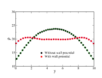
Figure 1: (Color online) Monomer density profiles with (squares) and without (circles) attractive wall potentials applied along the wall direction when particles approach close to walls. The dashed and dotted lines are the theoretical prediction described in Eq. (12) and Eq. (15), respectively. The spring constant of dumbbells and the collision time are $\mathrm{K}=0.2$ and $h=0.02$, respectively. Both simulations are with absence of shear flow.

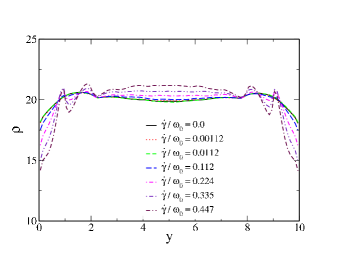
Figure 2: (Color online) Monomer density profiles at various dimensionless shear rates $\dot{\gamma}/\omega_{0}$, ranging from $\dot{\gamma}/\omega_{0}=0.0$ to $0.447$, when attractive wall potentials are applied. The spring constant of dumbbells and the collision time are as same as those in Fig. 1. The small ripples in the profile at large $\dot{\gamma}/\omega_{0}$ are due to inhomogeneities in the temperature profile, since velocity rescaling is not sufficiently efficient at high shear rates. The ripples to not appear for MPC-AT.

The simulated density profile shows excellent agreement with the analytical solution of Eqs. (II.4) and (15) (see Appendix). The factors $c_{1}$ and $c_{2}$ are chosen to obtain a nearly uniform density distribution. This is achieved for $c_{1}=1.3$ and $c_{2}=0.4$. As shown in Fig. 1, the densities of point particles at both wall boundaries deviate by less than $10\%$ lower from the bulk value, when the attractive wall potentials are applied. Simulations are also performed on systems of dumbbells with various spring constants, ranging from $\mathrm{K}a_{0}^{2}/k_{\mathrm{B}}T=0.1$ to $\mathrm{K}a_{0}^{2}/k_{\mathrm{B}}T=5.0$, in the absence of shear flow. It is found that for the given values of $c_{1}$ and $c_{2}$, the density profiles are essentially independent of the spring constant of the dumbbell in the range $0.1<\mathrm{K}a_{0}^{2}/k_{\mathrm{B}}T<1.0$. In Fig. 2, we plot density profiles in shear flow. At lower shear rates, i.e. $\dot{\gamma}/\omega_{0}\leq 0.1$, nearly identical profiles are obtained as without flow. For higher shear rates, deviations of the density profile from the equilibrium profile become significant. Nevertheless, these profiles are still more uniform than those without an attractive wall potential. Our investigations are mainly focusing on relatively low shear rates, where the non-uniformity of the density profile is not significant.

II.5 Stress Tensor and Shear Viscosity

In the MPC model, the viscosity $\eta$ consists of a kinetic and collisional contributionKikuchi et al. (2003); Tüzel et al. (2003). At steady shear rates, with flow along the $x$ direction and gradient along the $y$ direction, $\eta$ is calculated by measuring the $xy$ component of the stress tensor, $\sigma_{xy}=\sigma^{\mathrm{kin}}_{xy}+\sigma^{\mathrm{col}}_{xy}$, so that $\eta=\sigma_{xy}/\dot{\gamma}$.

In the streaming step, $\sigma^{\mathrm{kin}}_{xy}$ is proportional to the flux of the $x$ momentum crossing a plane normal to the $y$ direction. Since the stress tensor is independent of the position of the plane, we choose $y=0$ or $y=L_{y}$ to measure the momentum transfer. In two-dimensional simulations,

$$\sigma^{\mathrm{kin}}_{xy}=\frac{\mathrm{m}}{L_{x}h}\sum^{N_{1}}_{i=1}\left[v^{\prime}_{x,i}(t_{w})-v_{x,i}(t_{w})\right]\;,$$ (16)

where $t_{w}\in[t,t+h]$ is the time at which particle $i$ bounces back from the wall, $v_{x,i}(t_{w})$ and $v^{\prime}_{x,i}(t_{w})$ are the velocities just before and after the collision with the wall, and $N_{1}$ denotes the number of particles which hit one of the walls in the time interval $[t,t+h]$. In the collision step, particles close to the wall will change their velocities due to the multi-particle collisions with virtual wall particles with average velocity $v_{x}=\pm\frac{1}{2}\dot{\gamma}L_{y}$, so that

$$\sigma^{\mathrm{col}}_{xy}=\frac{\mathrm{m}}{L_{x}h}\sum^{N_{2}}_{i=1}\left[v^{\prime}_{x,i}(t+h)-v_{x,i}(t+h)\right]\;.$$ (17)

Here $N_{2}$ denotes the number of particles which have multi-particle collisions with virtual particles, while $v_{x,i}(t+h)$ and $v^{\prime}_{x,i}(t+h)$ are the velocities of particle $i$ before and after the collision step, respectively. In our simulations, $N_{2}$ is found to be much larger than $N_{1}$ for small collision times $h$, indicating that the collisional part dominates the shear viscosity. Simulations are first performed on a system of pure point-like fluid particles to verify the measurement of the zero-shear viscosity from Eqs. (16) and (17). We get perfect agreement with the theoretical predictionsKikuchi et al. (2003); Tüzel et al. (2003); Ripoll et al. (2005) for $\eta$.

The shear viscosity can also be measured from system under Poiseuille flowLamura et al. (2001); Ripoll (2006) by

$$\eta=\frac{\rho gL_{y}^{2}}{8v_{\mathrm{max}}}\;,$$ (18)

where $g$ is the gravitation field, and $v_{\mathrm{max}}$ the maximum flow velocity.

II.6 Storage and Loss Moduli

In an oscillatory shear flow, the shear rate $\dot{\gamma}(t)$ is time-dependent,

$$\dot{\gamma}(t)=\gamma_{0}~{}\omega~{}\cos{(\omega t)}\;,$$ (19)

where $\gamma_{0}$ and $\omega$ are the strain amplitude and the oscillation frequency, respectively. Note that the frequency $\omega$ in Eq. (19) is independent of the angular frequency $\omega_{0}$ of harmonic dumbbells in Section II. In our simulations, we choose $\gamma_{0}\ll 1$ in order to investigate the linear viscoelastic regime. The stress tensor is divided into two contributions, the viscous part $\sigma^{\prime}$ and the elastic part $\sigma^{\prime\prime}$, so thatLarson (1999); Macosko (1994)

$$\sigma_{xy}(t) = \sigma^{\prime}\sin{(\omega t)}+\sigma^{\prime\prime}\cos{(\omega t)}$$ (20)

$$= \gamma_{0}\left[G^{\prime}(\omega)\sin{(\omega t)}+G^{\prime\prime}(\omega)\cos{(\omega t)}\right]\;,$$

where $G^{\prime}$ is the storage modulus, which measures the in-phase storage of the elastic energy, and $G^{\prime\prime}$ is the loss modulus, which measures the out-of-phase energy dissipation. For a simple Maxwell fluid, $G^{\prime}$ and $G^{\prime\prime}$ are given byMacosko (1994)

$$G^{\prime} = G^{*}\frac{(\omega/\omega^{*})^{2}}{1+(\omega/\omega^{*})^{2}}\;;$$ (21)

$$G^{\prime\prime} = G^{*}\frac{\omega/\omega^{*}}{1+(\omega/\omega^{*})^{2}}\;\;,$$ (22)

where $\omega^{*}$ is a characteristic relaxation frequency, and $G^{*}$ is a characteristic shear modulus. In the limit of $\omega\ll\omega^{*}$, the loss modulus is $G^{\prime\prime}=\eta~{}\omega$, where $\eta$ is the zero-shear viscosity.

II.7 Kinetic Theory of Dumbbells in Solution

In order to estimate the rheological properties of our model fluid, we modify the kinetic theory for dilute solutions of elastic dumbbells Bird et al. (1987). For Hookean dumbbells in a solvent, the viscosity $\eta_{0}$, the storage modulus $G_{0}^{\prime}$ and the loss modulus $G_{0}^{\prime\prime}$ are given byBird et al. (1987)

$$\eta_{0}=\eta_{s}+\frac{\rho}{2}\,\frac{k_{B}T}{\omega_{s}},$$ (23)

$$G_{0}^{\prime}=\frac{\rho k_{B}T}{2}\,\frac{(\omega/\omega_{s})^{2}}{1+(\omega/\omega_{s})^{2}},$$ (24)

$$G_{0}^{\prime\prime}=\eta_{s}\omega+\frac{\rho k_{B}T}{2}\,\frac{\omega/\omega_{s}}{1+(\omega/\omega_{s})^{2}},$$ (25)

where

$$\omega_{s}=\frac{4\mathrm{K}}{\zeta_{s}}$$ (26)

with solvent viscosity $\eta_{s}$ and friction coefficient $\zeta_{s}$ of a monomer. Moreover, the expectation value for the square of the monomer separation, divided by its equilibrium value, is given byBird et al. (1987)

$$\frac{\langle r^{2}\rangle}{\langle r^{2}\rangle_{\rm eq}}=1+\frac{2}{3}(\dot{\gamma}/\omega_{s})^{2}.$$ (27)

In Ref. Bird et al., 1987, the friction coefficient is obtained from Stokes’ law for a bead of radius $r$ in the solvent, i.e. $\zeta_{s}=6\pi\eta_{s}r$. However, in the MPC dumbbell fluid, there exists no explicit solvent and the monomers are point particles instead of spheres. Nevertheless, the motion of the monomers is governed by the friction caused by the surrounding monomers which can be considered to take the role of the solvent. Using $\zeta=k_{B}T/D$, which follows from the Stokes-Einstein relation, we can thus relate the friction to the diffusion constant $D$ of a MPC fluid of point particles with the same monomer density. Similarly, we substitute the viscosity of the solvent, $\eta_{s}$, by the corresponding viscosity $\eta_{\rm MPC}$ of a MPC fluid of point particles. Theoretical expression for $\eta_{\rm MPC}$ and $D$ for the different collision methods can be found in Refs. Kikuchi et al., 2003; Tüzel et al., 2003; Götze et al., 2007; Noguchi and Gompper, 2007 and Refs. Ripoll et al., 2005; Tüzel et al., 2006; Noguchi and Gompper, 2007, respectively. The zero-shear viscosity then reads

$$\eta=\eta_{\rm MPC}+\frac{\rho}{2}\,\frac{k_{B}T}{\omega_{H}},$$ (28)

where we have introduced

$$\omega_{H}=\frac{4\mathrm{K}}{\zeta}=\frac{4D\mathrm{K}}{k_{B}T}.$$ (29)

Note that the limit $\mathrm{K}\rightarrow\infty$ corresponds to a MPC fluid of $N_{p}/2$ point particles of mass $\mathrm{m}^{\mathrm{c}}$. Here, the second term in Eq. (28) vanishes, and since $\eta_{\rm MPC}(\rho/2,2\mathrm{m})\approx\eta_{\rm MPC}(\rho,\mathrm{m})$ for not too small $\rho$ and sufficiently small $h$ (so that the collisional part of the viscosity dominates), the viscosity resulting from this simple theory approaches the correct value in this limit.

Consequently, we use the same substitutions for the storage and loss modulus, and for the average dumbbell extension, and obtain

$$G^{\prime}=\frac{\rho k_{B}T}{2}\,\frac{(\omega/\omega_{H})^{2}}{1+(\omega/\omega_{H})^{2}}$$ (30)

$$G^{\prime\prime}=\eta_{\rm MPC}\omega+\frac{\rho k_{B}T}{2}\,\frac{\omega/\omega_{H}}{1+(\omega/\omega_{H})^{2}},$$ (31)

and

$$\frac{\langle r^{2}\rangle}{\langle r^{2}\rangle_{\rm eq}}=1+\frac{2}{3}(\dot{\gamma}/\omega_{H})^{2}.$$ (32)

We emphasize that the above expressions only serve as a semi-quantitative description of the MPC dumbbell fluid. For example, the employed expressions for the diffusion constant neglect hydrodynamic interactions, which become important for small time steps $h$.

III Results

III.1 Dimensionless Variables and Parameters

In the remainder of this article, we introduce dimensionless quantities by measuring length in unit of the lattice constant $a_{0}$, mass in unit of the dumbbell mass $\mathrm{m}^{\mathrm{c}}$, time in units of $a_{0}\sqrt{\mathrm{m}^{\mathrm{c}}/k_{\mathrm{B}}T}$, velocity in units of $\sqrt{k_{\mathrm{B}}T/\mathrm{m}^{\mathrm{c}}}$, monomer number density $\rho$ in units of $a_{0}^{-d}$, where $d$ is the spatial dimension, and the spring constant $\mathrm{K}$ in units of $k_{\mathrm{B}}T/a^{2}_{0}$. The shear rate $\dot{\gamma}$ and all kinds of frequencies are measured in units of $\sqrt{k_{\mathrm{B}}T/\mathrm{m}^{\mathrm{c}}a^{2}_{0}}$. Finally the viscosity $\eta$ is in units of $\sqrt{\mathrm{m}^{\mathrm{c}}k_{\mathrm{B}}T/a^{2}_{0}}$, and the storage modulus $G^{\prime}$ and the loss modulus $G^{\prime\prime}$ are in units of $k_{\mathrm{B}}T/a^{3}_{0}$. In these dimensionless units, the mean free path $\lambda$ (in units of the lattice constant) becomes equivalent to the time step $h$.

In our simulations, harmonic dumbbells with $N_{\mathrm{p}}$ point particles are initially placed in a two- or three-dimensional rectangular box at random. We choose the average number density of point particles $\rho=20$ and $L_{x}=50$ for all two-dimensional simulations which results in $N_{\mathrm{p}}=1000L_{y}$. The collision time ranges from $h=0.01$ to $h=0.2$, while the spring constant ranges from $\mathrm{K}=0.1$ to $\mathrm{K}=5.0$. The rotational angle is chosen $\alpha=90^{\mathrm{o}}$ and $\alpha=130^{\mathrm{o}}$ for two- or three-dimensional simulations, respectively. We use small $h$ and large $\alpha$ to obtain large Schmidt numbers required for fluid-like behaviorRipoll et al. (2004, 2005). Most of the results shown are obtained from two-dimensional systems, except in a few cases where this is explicitly mentioned.

In Tab. 1, the theoretical values for the diffusion constant $D$ are given for $h=0.1$ for the different collision methods and various monomer densities Ripoll et al. (2005); Noguchi and Gompper (2007). The corresponding results for other time steps $h$ can be obtained by employing the linear relationship between $D$ and $h$.

$\rho$	$D^{\rm(SRD)}$	$D^{{\rm(AT}-a{\rm)}}$	$D^{{\rm(AT}+a{\rm)}}$
10	0.1222	0.1222	0.1353
20	0.1105	0.1105	0.1162
40	0.1051	0.1051	0.1078

Table 1: Diffusion constants $D$ of point-particle fluids for the standard MPC-SRD algorithm, as well as for MPC-AT$-a$ and MPC-AT$+a$ simulations for various monomer densities, in two dimensions. All data are calculated for collision time $h=0.1$. Diffusion constants for other time steps $h$ can be obtained by employing the linear relationship between $D$ and $h$. Note that the values for MPC-AT$-a$ are identical with those for MPC-SRD with collision angle $\alpha=90^{\mathrm{o}}$.

III.2 Steady Shear Flow

Figure 3: (Color online) Snapshots of dumbbell configurations in steady shear flow. The system size is $L_{x}=L_{y}=50$. Half of each dumbbell is colored red, the other half yellow for reason of visualization. In each frame only 2500 dumbbells are shown, so that the density is $10$ times as high as appears from the pictures. The spring constant and the collision time are $\mathrm{K}=0.2$ and $h=0.02$, respectively. From (A) to (D), the applied shear rates are $\dot{\gamma}/\omega_{H}=0.0565$, $0.565$, $2.83$ and $5.65$.

In Fig. 3, we present snapshots for steady shear flow with a simulation box containing 25000 dumbbells. At lower shear rates, i.e. $\dot{\gamma}/\omega_{H}\leq 0.6$, see Fig. 3A and 3B, the average extension of the dumbbells is hardly distinguishable from the equilibrium value. In these two cases, the shear flow is not strong enough to align the dumbbells along the flow direction, so that both systems are still isotropic. With increasing $\dot{\gamma}$, shear forces overwhelm entropic forces. As a result, dumbbells are largely stretched, at the same time reorientated along the flow direction, as presented in Fig. 3C and 3D. Note that near both the walls, the average size $\langle\mathrm{r^{2}}\rangle^{1/2}$ of the dumbbells in flow is larger than in the bulk. Also, an alignment of the dumbbells is found near the walls, both with and without shear flow, with peaks at $y=0$ and $y=L_{y}$. This is an effect of the geometrical constraints imposed on anisotropic particles by a hard wall. Furthermore, a maximum of the extension occurs at a finite distance from the wall, which we attribute to the combined effect of the wall and the flow conditions; dumbbells very close to the wall are sterically oriented parallel to the wall and thus experience only a very small shear force, while those a little further away are close to the average inclination angle (see Fig. 4 below), which corresponds to the largest stretching. The distance of the position of the maximum from the wall decreases with increasing shear rate, and seems to approach the size of the collision cells for large $\dot{\gamma}$. The relative peak height increases with increasing shear rate. For example, we find that the maximum extension $\langle\mathrm{r^{2}}\rangle^{1/2}$ near the wall is about $11\%$ larger than the bulk extension for $\dot{\gamma}/\omega_{H}=1.13$, while it is about $28\%$ larger than in the bulk for $\dot{\gamma}/\omega_{H}=2.83$.

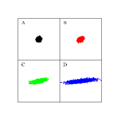
Figure 4: (Color online) Distribution of dumbbell configurations for the system shown in Fig. 3. Each dot indicates the end-to-end vector of a dumbbell.

Fig. 4 presents the extensional and orientational distribution of the dumbbells for various shear rates. At lower shear rates, $\dot{\gamma}/\omega_{H}\leq 1$, the end-to-end vector of the dumbbells is distributed on a circle, see Fig. 4A and B, indicating an isotropic orientation. At a higher shear rate, $\dot{\gamma}/\omega_{H}=2.83$, the orientational distribution becomes an elongated ellipse, see Fig. 4C. With increasing shear rate, the distribution elongates further. Simultaneously, dumbbells become more aligned with the flow direction, as can be seen quantitatively from the inclination angle $\theta$ shown in Fig. 5. Here, the inclination angle is defined as the angle between the average orientation of the end-to-end vector of a dumbbell and the the flow direction. At lower shear rates, $\dot{\gamma}/\omega_{H}\leq 1$, the inclination angle approaches $\theta=45^{\mathrm{o}}$, while it decays to zero for large shear rates with a power law $\dot{\gamma}^{-1}$.

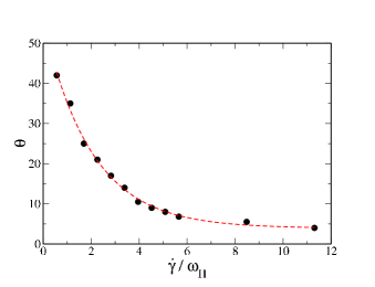
Figure 5: (Color online) The inclination angle $\theta$ as a function of dimensionless shear rate $\dot{\gamma}/\omega_{H}$ for the system of Fig. 3, with spring constant $\mathrm{K}=0.2$, collision time $h=0.02$, and system size $L_{x}=L_{y}=50$.

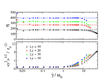
Figure 6: (Color online) Shear viscosity $\eta$ and scaled average dumbbell length $\langle\mathrm{r}^{2}\rangle^{1/2}/\mathrm{r}_{0}^{(2)}$ as a function of dimensionless shear rate $\dot{\gamma}/\omega_{H}$. Systems with the wall separation $L_{y}=10,~{}20,~{}30$, and $50$ are investigated. The spring constant is $\mathrm{K}=0.2$ and the collision time $h=0.02$.

In Fig. 6, we plot the shear viscosity $\eta$ as a function of dimensionless shear rate $\dot{\gamma}/\omega_{H}$ for various wall separations $L_{y}$ ranging from $10$ to $50$. In each system, $\eta$ remains constant until the applied shear rate reaches a critical value $\dot{\gamma}_{c}/\omega_{H}\approx 5$. The shear viscosity then decays rapidly as $\dot{\gamma}$ further increases, showing a typical “shear-thinning” behavior. Fig. 6 also shows the average extension of dumbbells $\langle\mathrm{r}^{2}\rangle^{1/2}/\mathrm{r}_{0}^{(2)}$ as a function of the shear rate.

Two comments are required here. Firstly, in our MPC model, an entanglement between dumbbells is not taken into account, so that they can freely cross each other. Also, the absence of an excluded-volume interaction implies that there is no benefit of a para-nematic ordering in terms of an increased sliding of parallel dumbbells along each other as in solutions of rod-like colloids; instead, parallel dumbbells interact very similarly to isotropically oriented dumbbells, since in both cases the monomers colloide with other monomers in exactly the same fashion. Thus, our system is very similar to a solution of non-interacting harmonic dumbbells, for which – in the absence of a finite extensibility – neither “shear-thinning” nor “shear-thickening” is expectedBird et al. (1987); Doi and Edwards (1986), compare Eq. (23). Secondly, the size of the simulation box should have no influence on the bulk viscosity at a given shear rate. However, the plateau value of the viscosity increases strongly with the wall separation $L_{y}$. This indicates that boundary effects could be responsible for the observed “shear-thinning” behavior.

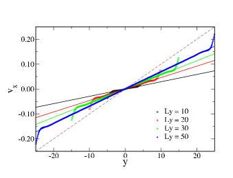
Figure 7: (Color online) Velocity profiles for wall separations $L_{y}=10$, $20$, $30$, and $50$. Data are obtained for spring constant $\mathrm{K}=0.2$, collision time $h=0.02$, and shear rate $\dot{\gamma}/\omega_{H}=0.565$. The dashed line corresponds to the applied shear rate. Solid lines represent fits to the bulk part of the velocity profiles, their slopes yield the effective shear rates $\dot{\gamma}_{\mathrm{eff}}$.

We therefore examine the velocity profiles for systems with various wall separations $L_{y}$. In Fig. 7, the average velocities $v_{x}$ of the monomers along the flow direction are plotted as function of $L_{y}$ for a fixed shear rate of $\dot{\gamma}/\omega_{H}=0.565$. The velocities at the boundaries deviate only very little from the wall velocities, i.e. there is very little slip at the walls, as expected. However, the velocity decays rapidly in a boundary layer of thickness $\Delta$, then decays linearly to zero at the middle plane. Obviously the applied shear rate $\dot{\gamma}$ is not appropriate to calculate the shear viscosities from the stress tensor $\sigma_{xy}$ by $\eta=\sigma_{xy}/\dot{\gamma}$. An effective shear rate $\dot{\gamma}_{\mathrm{eff}}$ is therefore introduced instead, which characterizes the linear bulk part of the velocity profile. At a given shear rate, the larger the wall separation, the less the effective shear rate deviates from $\dot{\gamma}$, since the finite-size effect is much stronger in smaller systems. The ratio $\dot{\gamma}/\dot{\gamma}_{\mathrm{eff}}$ between the applied and the effective shear rates is plotted in Fig. 8, as a function of $\dot{\gamma}/\omega_{H}$. At lower shear rates, i.e. $\dot{\gamma}<\dot{\gamma}_{\mathrm{c}}$, where $\dot{\gamma}_{\mathrm{c}}$ is the critical shear rate, the ratio $\dot{\gamma}/\dot{\gamma}_{\mathrm{eff}}$ is independent of the shear rate. When the applied shear rate becomes larger than this critical value, the effective shear rate $\dot{\gamma}_{\mathrm{eff}}$ increases more slowly than $\dot{\gamma}$.

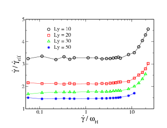
Figure 8: (Color online) Ratios between the applied shear rates $\dot{\gamma}$ and the effective shear rates $\dot{\gamma}_{\mathrm{eff}}$ as a function of $\dot{\gamma}/\omega_{H}$ for the same systems as in Fig. 6.

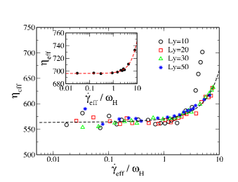
Figure 9: (Color online) Master curve of the viscosity $\eta_{\mathrm{eff}}$ as a function of the effective shear rate $\dot{\gamma}_{\mathrm{eff}}$ on a semi-logarithmic scale. Symbols are the same as in Fig. 6 and Fig. 8. For strong shear flow, i.e. $\dot{\gamma}_{\mathrm{eff}}/\omega_{H}\gtrsim 2$, the viscosity increases (“shear thickening”). The dashed line is fitted to the data with wall separations $L_{y}\geq 20$. In the inset, $\eta_{\mathrm{eff}}$ is plotted as a function of $\dot{\gamma}_{\mathrm{eff}}/\omega_{H}$ for three-dimensional systems. A $20\times 20\times 10$ simulation box is chosen, while the spring constant $\mathrm{K}$, the collision time $h$ and the average number density $\rho$ are the same as in the two-dimensional systems.

Consequently, the effective shear viscosity can be calculated by

$$\eta_{\mathrm{eff}}=\frac{\sigma_{xy}}{\dot{\gamma}_{\mathrm{eff}}}\;.$$ (33)

In Fig. 9, $\eta_{\mathrm{eff}}$ is shown against $\dot{\gamma}_{\mathrm{eff}}/\omega_{H}$ for various wall separations $L_{y}$. The data for different system sizes now all fall onto a single master curve, which describes the bulk shear viscosity. Now, instead of “shear thinning” shown in Fig. 6, a very weak “shear thickening” behavior is observed when $\dot{\gamma}_{\mathrm{eff}}/\omega_{H}>1$. Three-dimensional simulations are also carried out for systems of $20\times 20\times 10$ boxes along the $x$, $y$, and $z$ directions. For the same parameters $\mathrm{K}=0.2$ and $h=0.02$, weak “shear thickening” behavior is also observed, as shown in the inset of Fig. 9, when $\dot{\gamma}_{\mathrm{eff}}/\omega_{H}$ reaches the critical value, $\dot{\gamma}_{\mathrm{c},\mathrm{eff}}/\omega_{H}\approx 2$. The value of the critical shear rates are found to be very similar in two and three dimensions.

Fig. 9 shows that the effective shear viscosity $\eta_{\mathrm{eff}}$ is nearly independent of the shear rate for $\dot{\gamma}_{\mathrm{eff}}/\omega_{H}\leq\dot{\gamma}_{\mathrm{c,eff}}/\omega_{H}\approx 2$. This critical shear rate corresponds to the onset of the apparent “shear thinning” observed in Fig. 6, as well as the deviation of $\dot{\gamma}/\dot{\gamma}_{\mathrm{eff}}$ from its low-shear-rate value in Fig. 8. It should be noticed that the value of $\dot{\gamma}_{\mathrm{c},\mathrm{eff}}/\omega_{H}\approx 2$ implies $\dot{\gamma}_{\mathrm{c}}/\omega_{H}$ is in the range $[3,6.4]$ for system sizes $L_{y}\in[10,50]$, compare Fig. 8. However, it is important to note that there is already a pronounced alignment and stretching of the dumbbells for smaller shear rates; Fig. 5 shows that the inclination angle $\theta$ has decreased from $\theta=45^{\mathrm{o}}$ in the absence of shear flow to $\theta\approx 15^{\mathrm{o}}$ at $\dot{\gamma}/\omega_{H}=3$, while Fig. 6 indicates that $\langle\mathrm{r}^{2}\rangle^{1/2}/\mathrm{r}_{0}^{(2)}\approx 2$ at $\dot{\gamma}/\omega_{H}=3$.

The spring constant $\mathrm{K}$ of the dumbbells is of great importance, since it controls the elasticity of the fluid. We have therefore examined velocity profiles of systems of dumbbells with various spring constants. In Fig. 10, the simulation results are plotted for a fixed applied shear rate $\dot{\gamma}=0.01$. The effect of the boundary layer becomes more pronounced with decreasing spring constant. By fitting the linear parts of the velocity profiles, we find that, for the same shear rate $\dot{\gamma}=0.01$, the effective shear rate $\dot{\gamma}_{\mathrm{eff}}$ for dumbbells with $\mathrm{K}=0.1$ is about 10 times lower than that with the highest spring constant studied here, $\mathrm{K}=4.0$. The thickness of the boundary layer is proportional to the equilibrium average extension $\mathrm{r}_{0}^{(2)}=\sqrt{2k_{\mathrm{B}}T/\mathrm{K}}$, as shown in the inset of Fig. 10.

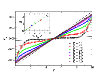
Figure 10: (Color online) Velocity profiles for various spring constants, ranging from $\mathrm{K}=0.1$ to $\mathrm{K}=4.0$. The wall separation in each case is $L_{y}=10$. The dashed line corresponds to the applied shear rate $\dot{\gamma}=0.01$, while solid lines are the fitted effective velocity profiles. The inset shows the thickness of the boundary layer $\Delta$ as a function of equilibrium extension $\mathrm{r}_{0}^{(2)}=\sqrt{2k_{\mathrm{B}}T/\mathrm{K}}$. The dashed line is a linear fit.

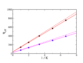
Figure 11: (Color online) The zero-shear viscosity $\eta_{\mathrm{eff}}$ as a function of spring constant $\mathrm{K}$ in both two-dimensional (circles) and three-dimensional (squares) systems. The solid lines are linear fits, the dashed lines indicate the theoretical predictions (28). In all simulations, the collision time is $h=0.02$. Two-dimensional simulations are performed in systems of $50\times 10$ boxes, while three-dimensional simulations are in $30\times 30\times 20$ boxes along the $x$, $y$ and $z$ directions, respectively. The average number density in three-dimensional systems is $\rho=10$, which is half of value in two-dimensional systems.

The zero-shear viscosity $\eta_{\mathrm{eff}}$ is found to depend linearly on $1/\mathrm{K}$, see Fig. 11. As $\mathrm{K}$ increases, the effective viscosity $\eta_{\mathrm{eff}}$ approaches the expected value of system of point particles with mass of $\mathrm{m}^{\mathrm{c}}$ and density $\rho/2$. The same linear relationship between $\eta_{\mathrm{eff}}$ and $1/\mathrm{K}$ is also obtained in three-dimensional systems, as shown in Fig. 11. Not only the linear dependence of $\eta_{\mathrm{eff}}$ on $1/\mathrm{K}$ but also the prefactors are in very good agreement with the theoretical predictions (28).

The scaled mean free path $\lambda$, which determines how far a point particle travels between collisions, is another important parameter which affects the shear viscosity. We always employ small mean free pathsRipoll et al. (2004, 2005), so that the collisional viscosity is dominant compared to the kinetic viscosity. The data of Fig. 12(a) demonstrate that the zero-shear viscosity increases linearly with $1/\lambda$, for all spring constants $\mathrm{K}$ studied here, as it does for a system of point particlesKikuchi et al. (2003); Tüzel et al. (2003); Ripoll et al. (2005). However, the slope decreases with increasing $\mathrm{K}$, in good agreement with the analytical results obtained from Eq. (28), as shown in the inset of Fig. 12(a).

Figure 12: (Color online) The effective shear viscosity $\eta_{\mathrm{eff}}$ as a function of the dimensionless effective shear rate $\dot{\gamma}_{\mathrm{eff}}/\omega_{0}$, on a double-logarithmic scale. (a) For fixed spring constant $\mathrm{K}=0.2$ and various mean free paths $\lambda=0.01$, $0.02$, $0.05$, $0.1$ and $0.2$. (b) For fixed mean free path $\lambda=0.02$ and various spring constants $\mathrm{K}=0.2$, $0.5$, $1.0$ and $5.0$. In both cases, the wall separation is $L_{y}=10$. The inset in (a) shows the zero-shear viscosity $\eta_{\mathrm{eff}}$ as a function of $1/\lambda$. The solid line indicates the theoretical result for $\mathrm{K}\rightarrow\infty$, while the other lines show the predictions (28) for $\mathrm{K}=0.2$, $0.5$, and $5.0$.

The weak “shear-thickening” behavior is observed for all mean free paths investigated here, see Fig. 12. Thus, this weak “shear-thickening” behavior is intrinsic to the MPC algorithm, and cannot be avoided by a variation of the collision time. Fig. 12(a) indicates that the critical shear rate $\dot{\gamma}_{\mathrm{c,eff}}/\omega_{0}$ depends only very weakly on the mean free path $\lambda$. Therefore, we present the simulation data in Fig. 12 as a function of $\dot{\gamma}_{\mathrm{eff}}/\omega_{0}$, since $\omega_{0}=(2\mathrm{K}/m)^{1/2}$ is independent of $\lambda$, while $\omega_{H}$ decreases linearly with $\lambda$. The “shear-thickening” behavior becomes more pronounced and slowly shifts to smaller values of $\dot{\gamma}_{\mathrm{eff}}/\omega_{0}$ for system of dumbbells with smaller spring constants, see Fig. 12(b). In the range of investigated spring constants and mean free paths, the shear thickening occurs roughly at $\dot{\gamma}_{\mathrm{c,eff}}/\omega_{0}\simeq 0.1$. It is important to note that the viscosity of the standard point-particle MPC fluid is also not independent of the shear rate, but shows a weak shear-thinning behavior at high shear rates Kikuchi et al. (2003). For our model parameters and in two dimensions, this shear-thinning behavior sets in at a shear rate $\dot{\gamma}_{\mathrm{c}}\simeq 1$. Thus, with increasing $\mathrm{K}$, shear thickening occurs at a slowly increasing $\dot{\gamma}_{\mathrm{c,eff}}/\omega_{0}$ for $\mathrm{K}\leq 1$; for larger spring constants $\mathrm{K}\geq 5$, shear thinning is observed instead, and $\dot{\gamma}_{\mathrm{c,eff}}/\omega_{0}$ decreases again (since $\dot{\gamma}_{\mathrm{c,eff}}\to 1$ and $\omega_{0}\to\infty$ for $\mathrm{K}\to\infty$).

III.3 Small-amplitude Oscillatory Shear Flow

Another way to explore the viscoelastic properties of a fluid is to apply a small-amplitude oscillatory shear flow. We use here the strain amplitudes $\gamma_{0}=\dot{\gamma}/\omega$ in the range $0.1$ to $0.5$ to mimic a small amplitude shearing. The frequencies $\omega$ ranges from $10^{-4}$ to $10^{-1}$ in our simulations, which provides a wide range of shear rate from $10^{-5}$ to $5\times 10^{-2}$.

The storage and loss moduli as a function of oscillation frequency are plotted in Fig. 13. Similarly to the simulations of steady shear flow, effective shear rates are measured from the bulk velocity profiles at times when $\cos(\omega t)=\pm 1$. By doing so, all the simulation data fall onto master curves at various wall separations from $L_{y}=10$ to $50$. As can been seen from Fig. 13(a), the storage modulus $G^{\prime}$ is well fitted by Eq. (21), indicating that the dumbbell system exhibits a typical behavior of a Maxwell fluid. The relaxation frequency $\omega^{*}$ obtained from the fit of the storage modulus $G^{\prime}$ against $\omega$ is then used in Eq. (22) to fit the loss modulus $G^{\prime\prime}$. In Fig. 13(b), at low frequencies, $\omega\leq 0.02$, the simulation data follow the expected linear $\omega$-dependence very well. In this linear regime, the shear viscosity is then calculated by $\eta=G^{\prime\prime}(\omega)/\omega$, which yields $\eta=565$, in excellent agreement with the result in steady shear flow, compare Fig. 9. Note that the fitted values for the amplitude $G^{*}$ in Eqs. (21) and (22) differ by about a factor 2. This indicates that the system investigated here does not behave exactly like a simple Maxwell fluid.

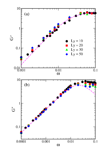
Figure 13: (Color online) (a) Storage $G^{\prime}$ and (b) loss modulus $G^{\prime\prime}$, as a function of oscillation frequency $\omega$ on a double-logarithmic scale, for systems with various wall separations ranging from $L_{y}=10$ to $50$. The spring constant and the collision time are $\mathrm{K}=0.2$ and $h=0.02$, respectively. The dashed line in (a) is fitted by the Maxwell model, Eq. (21), on the basis of all simulation data, while the one shown in (b) is based on data for oscillation frequencies $\omega<0.02$.

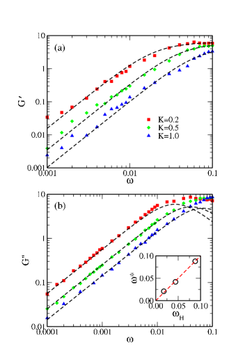
Figure 14: (Color online) (a) The storage $G^{\prime}$ and (b) the loss moduli $G^{\prime\prime}$, as function of oscillation frequency $\omega$ on a double-logarithmic scale, for systems of dumbbells with various spring constants ranging from $\mathrm{K}=0.2$ to $\mathrm{K}=1.0$. The wall separation and the collision time are $L_{y}=10$ and $h=0.02$, respectively. The inset shows the fitted relaxation frequencies $\omega^{*}$ as a function of the frequency $\omega_{H}$ predicted by Eq. (29). The dashed line shows the identity $\omega^{*}=\omega_{H}$.

In Fig. 14, we examine the storage and loss moduli of system of dumbbells with various spring constants. As in Fig. 13, simulation results are all well fitted by the Maxwell equations (21) and (22), except for somewhat different amplitudes $G^{*}$. The relaxation frequency $\omega^{*}$ is found to agree very well with $\omega_{H}$, as shown in the inset of Fig. 14. At lower oscillation frequency in Fig. 14(b), the viscosities calculated from $G^{\prime\prime}(\omega)/\omega$ are $\eta=565$, $253$ and $144$ for systems with $\mathrm{K}=0.2$, $0.5$ and $1.0$, respectively. These values are again in excellent agreement with those calculated from Eq. (33) in steady shear flow. For all spring constants $\mathrm{K}$, the fitted amplitudes $G^{*}$ for the storage moduli $G^{\prime}$ are about half of those calculated for the loss moduli $G^{\prime\prime}$. This indicates that even for a system of dumbbell with high spring constant, a simple Maxwell model is not appropriate for a quantitative description.

III.4 Angular Momentum Conservation

The viscosity of a simple MPC-AT$+a$ fluid (with angular-momentum conservation) is about a factor $1/2$ smaller than of a MPC-AT$-a$ fluid Götze et al. (2007); Noguchi and Gompper (2007). We thus expect the viscosity of the dumbbell fluid to be affected by angular-momentum conservation as well. The simulation results for both MPC-AT$-a$ and MPC-AT$+a$ methods are compared in Fig. 15. We find that the effective zero-shear viscosity $\eta_{\rm eff}$ increases linearly with the monomer density $\rho$ for $\rho\gtrsim 5$. The corresponding theoretical results (28) are in good agreement with the simulation results for both investigated spring constants. Minor deviations from the linear relationship of $\eta_{\rm eff}$ with $\rho$ originate from the variation of the diffusion constant at low densities, which approaches a constant value for high $\rho$. The viscosity of MPC-AT$+a$ is lower than for MPC-AT$-a$, although this effect is less pronounced than for pure point-particle MPC fluids, since the main contribution to the viscosity originates from the spring tension.

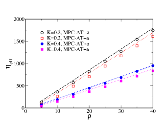
Figure 15: (Color online) Effective shear viscosities $\eta_{\rm eff}$ as a function of the density $\rho$ for MPC-AT$-a$ and MPC-AT$+a$, each for spring constants $\mathrm{K}=0.2$ and $\mathrm{K}=0.4$. The lines represent the theoretical results obtained from Eq. (28). The wall separation and the collision time are $L_{y}=20$ and $h=0.014$, respectively.

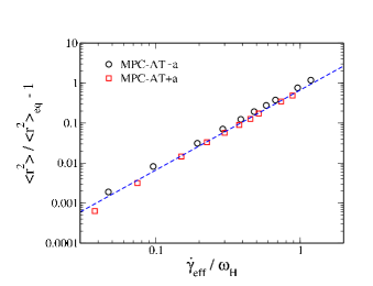
Figure 16: (Color online) Scaled average of the dumbbell extension, $\langle r^{2}\rangle/\langle r^{2}\rangle_{\rm eq}-1$, as a function of the effective shear rate $\dot{\gamma}_{\mathrm{eff}}/\omega_{H}$ for angular-momentum conserving and non-conserving methods. The spring constant and collision time are $\mathrm{K}=0.2$ and time step $h=0.014$, respectively, the density is $\rho=10$ and the wall separation is $L_{y}=20$. The dashed line represents the theoretical result (32).

In Fig. 16, we present the average squared dumbbell extension, determined in the bulk as a function of the effective shear rate, along with the theoretical results (32), for both the MPC-AT$-a$ and MPC-AT$+a$ methods. Note that the diffusion constant $D$ in Eq. (32) is different for angular-momentum conserving and non-conserving methods. The angular-momentum conservation has only little effect on the spring extension; for a given effective shear rate, the extension is slightly lower for the angular-momentum conserving method. The agreement of the simulation data with the theoretical result (32) is again remarkably good.

IV Discussion

As a further test for the correct calculation of the effective viscosity by the procedure described in Secs. II.5 and III.2, we have also determined the viscosity from Poiseuille flow. As in Ref. Allahyarov and Gompper, 2002, we apply a gravitational force of strength $g$ parallel to the walls, with $g$ in the range from $g=0.0001$ to $g=0.01$ (in units of $k_{\mathrm{B}}T/a_{0}$). We fit the central part of the velocity profile to a parabolic flow curve. The value of this curve at the wall positions determines the effective wall slip. When this slip velocity is subtracted, Eq. (18) in Sec. II.5 is employed to determine the viscosityZhang et al. (2007). We have used this method for a system of dumbbells with $\mathrm{K}=0.2$ in a $30\times 30$ box. Excellent agreement between the two methods to calculate the zero-shear viscosity is obtained.

Our results for the dependence of the inclination angle $\theta$ on the shear rate can be compared with the decay of the inclination angle of flexible and semi-flexible polymers. For dilute polymer solutions in the asymptotic regime of high shear rates (where the finite extensibility is important), $\theta$ has been predicted from Brownian dynamics simulations Schroeder et al. (2005) and theory Winkler (2006) to decay with a power law $\dot{\gamma}^{-0.3}$ and $\dot{\gamma}^{-1/3}$, respectively. For extensible dumbbells, the theory of Ref. Winkler, 2006 predictsWinkler (2007) $\theta\sim\dot{\gamma}^{-1}$, in excellent agreement with our simulation results.

The wall slip in polymer melts has been studied extensively. In this case, molecular dynamics simulations of polymer fluids with Lennard-Jones interactions between monomers give a wall slip with a boundary layer thickness, which is on the order of the monomer diameter $\sigma$ or less Priezjev and Troian (2004); Zhang et al. (2007). Our model could be compared more easily with results for polymer solutions, because our model does not include excluded-volume interactions. However, there is little knowledge about semi-dilute polymer solutions near a wall under flow conditions. Nevertheless, some comparisons with polymer melts with moderate chain lengths are possible, where entanglement effects are absent. For example, the molecular dynamics simulations of Zhang et al.Zhang et al. (2007) show a maximum of mean squared radius of gyration at a finite distance $\Delta_{m}$ from the wall, which shifts from $\Delta_{m}\simeq 1.5\sigma$ for chains with $4$ monomers to $\Delta_{m}\simeq 2.2\sigma$ for $10$ monomers.

V Summary and Conclusions

A multi-particle collision dynamics (MPC) algorithm has been developed to investigate the viscoelastic properties of harmonic-dumbbell fluid in shear flow. The method is based on alternating streaming and collision steps, just as the original MPC method for Newtonian fluids. The only modification is to replace the ballistic motion of fluid point particles by harmonic oscillations during the streaming step. In this model, the entanglement between dumbbells is neglected. Moreover, the storage and loss moduli are calculated by introducing a small amplitude oscillatory shear flow.

Our results can be summarized as follows:

First, under steady shear flow, the dumbbells keep their isotropic distribution at low shear rates, but get highly stretched and orientated along the flow direction at high shear rates. The velocity profile is not uniform along the gradient direction, but boundary layers of high shear develop near the walls. The thickness of these boundary layers is found to scale with the size of the dumbbells in the absence of flow. The effective shear viscosity, calculated from the ratio between the off-diagonal component of the stress tenor, $\sigma_{xy}$, and the effective shear rate $\dot{\gamma}_{\mathrm{eff}}$, expresses a very weak “shear thickening” behavior at high shear rates.

Second, the dependence of the viscosity on two parameters, the spring constant $\mathrm{K}$ of the dumbbells and the collision time $h$, has been investigated. These two parameters are of central importance, since the former controls the elastic energy of the system, while the latter determines the mean free path $\lambda$, which measures the fraction a the cell size that a fluid particle travels on average between collisions. We find that the shear viscosity of the dumbbell fluid increases linearly with $1/\mathrm{K}$ and with $h$.

Third, the storage and loss moduli of our viscoelastic solvent are studied by imposing an oscillatory velocity on the two solid walls. The storage modulus $G^{\prime}$ is found to be proportional to $\omega^{2}$ at low frequencies, and to level off at $\omega^{*}=\omega_{H}$. Its behavior over the whole frequency range studied here is well described by a Maxwell fluid. The loss modulus $G^{\prime\prime}$ increases linearly with $\omega$ for low frequencies. The shear viscosities obtained from the ratio $G^{\prime\prime}/\omega$ at low shear rates agree very well with those obtained from simulations with steady shear. On the other hand, for $\omega>\omega_{H}$, we find that the data approach a plateau value, while for a Maxwell fluid $G^{\prime\prime}$ would decrease again for higher frequencies.

Our numerical results are quantitatively in good agreement with a simple theory, based on the kinetic theory of dilute solutions of dumbbells, where the transport coefficients of the standard MPC point-particle fluid are employed for the viscosity and the diffusion constant of the solvent.

In our MPC algorithm of harmonic dumbbells, both elastic and viscous behaviors of solvent particles can be modeled properly, while hydrodynamic interactions are efficiently taken into account. These are valuable assets to guide future simulations on investigating rheological properties of suspensions of spherical, rod-like or polymeric solute molecules in viscoelastic fluids.

Appendix: Analytical solution of the density profile with attractive wall potentials

Combining Equations (II.4) and (15), the density profile, when attractive wall potentials are introduced, can be solved analytically. Considering the symmetry of the density profile, $\rho(y)=\rho(L_{y}-y)$, only the initial half part need to be taken into account. For $0<y<2c_{1}\mathrm{r}_{0}^{(1)}$, we then arrive at

$$\rho(y) = \frac{1}{Z}\left\{\int^{L_{y}}_{0}dy^{\prime}~{}\mathrm{e}^{-\mathrm{K}(y-y^{\prime})^{2}/2k_{\mathrm{B}}T}\right.$$

$$+ \left.\int^{2c_{1}\mathrm{r}_{0}^{(1)}-y}_{0}dy^{\prime}~{}\mathrm{e}^{-\-\mathrm{K}(y-y^{\prime})^{2}/2k_{\mathrm{B}}T}~{}\left[~{}\mathrm{e}^{2c_{2}k_{\mathrm{B}}T(1-(y+y^{\prime})/2c_{1}\mathrm{r}_{0}^{(1)}~{})}-1~{}\right]\right\}\;.$$

which implies

$$\rho(y) = \frac{1}{Z}\left\{\mathrm{erf}\left(\sqrt{\mathrm{K}/2k_{\mathrm{B}}T}~{}(L_{y}-y)\right)+\mathrm{erf}\left(\sqrt{\mathrm{K}/2k_{\mathrm{B}}T}~{}(2y-2c_{1}\mathrm{r}_{0}^{(1)})\right)\right.$$

$$+ \left.\exp\left[\frac{(c_{2}k_{\mathrm{B}}T\mathrm{r}_{0}^{(1)})^{2}+4c_{2}k_{\mathrm{B}}T(c_{1}\mathrm{r}_{0}^{(1)}-y)}{2c_{1}\mathrm{r}_{0}^{(1)}}\right]\left[\mathrm{erf}\left(\frac{-c_{2}k_{\mathrm{B}}T+c_{1}\mathrm{r}_{0}^{(1)}y\mathrm{K}/k_{\mathrm{B}}T}{c_{1}\mathrm{r}_{0}^{(1)}\sqrt{2\mathrm{K}/k_{\mathrm{B}}T}}\right)\right.\right.$$

$$+ \left.\left.\mathrm{erf}\left(\frac{c_{2}k_{\mathrm{B}}T+2(c_{1}\mathrm{r}_{0}^{(1)}-y)c_{1}\mathrm{r}_{0}^{(1)}\mathrm{K}/k_{\mathrm{B}}T}{c_{1}\mathrm{r}_{0}^{(1)}\sqrt{2\mathrm{K}/k_{\mathrm{B}}T}}\right)\right]\right\}\;,$$

while for $2c_{1}\mathrm{r}_{0}^{(1)}<y<L_{y}/2$, the density profile is given by Eq. (13).

References

- Larson (1999) R. G. Larson, The Structure and Rheology of Complex Fluids (Oxford University Press, New York, 1999).
- Ferry (1980) J. D. Ferry, Viscoelastic Properties of Polymers (Wiley, New York, 1980).
- Doi and Edwards (1986) M. Doi and S. F. Edwards, The Theory of Polymer Dynamics (Clarendon Press, Oxford, 1986).
- Malevanets and Kapral (1999) A. Malevanets and R. Kapral, J. Chem. Phys. 110, 8605 (1999).
- Malevanets and Kapral (2000) A. Malevanets and R. Kapral, J. Chem. Phys. 112, 7260 (2000).
- Lamura et al. (2001) A. Lamura, G. Gompper, T. Ihle, and D. M. Kroll, Europhys. Lett. 56, 319 (2001).
- Ihle and Kroll (2001) T. Ihle and D. M. Kroll, Phys. Rev. E 63, 020201(R) (2001).
- Mussawisade et al. (2005) K. Mussawisade, M. Ripoll, R. G. Winkler, and G. Gompper, J. Chem. Phys. 123, 144905 (2005).
- Lee and Kapral (2006) S. H. Lee and R. Kapral, J. Chem. Phys. 124, 214901 (2006).
- Webster and Yeomans (2005) M. A. Webster and J. M. Yeomans, J. Chem. Phys. 122, 164903 (2005).
- Ryder and Yeomans (2006) J. F. Ryder and J. M. Yeomans, J. Chem. Phys. 125, 194906 (2006).
- Ripoll et al. (2006) M. Ripoll, R. G. Winkler, and G. Gompper, Phys. Rev. Lett. 96, 188302 (2006).
- Padding and Louis (2004) J. T. Padding and A. A. Louis, Phys. Rev. Lett. 93, 220601 (2004).
- Hecht et al. (2005) M. Hecht, J. Harting, T. Ihle, and H. J. Herrmann, Phys. Rev. E 72, 011408 (2005).
- Noguchi and Gompper (2004) H. Noguchi and G. Gompper, Phys. Rev. Lett. 93, 258102 (2004).
- Noguchi and Gompper (2005) H. Noguchi and G. Gompper, Phys. Rev. E 72, 011901 (2005).
- Tucci and Kapral (2004) K. Tucci and R. Kapral, J. Chem. Phys. 120, 8262 (2004).
- Echeveria et al. (2007) C. Echeveria, K. Tucci, and R. Kapral, J. Phys.: Condens. Matter 19, 065146 (2007).
- Helfand and Fredrickson (1989) E. Helfand and G. H. Fredrickson, Phys. Rev. Lett. 62, 2468 (1989).
- Onuki (1989) A. Onuki, Phys. Rev. Lett. 62, 2472 (1989).
- Milner (1993) S. T. Milner, Phys. Rev. E 48, 3674 (1993).
- Tanaka (2000) H. Tanaka, J. Phys.: Condens. Matter 12, R207 (2000).
- Groisman and Steinberg (2000) A. Groisman and V. Steinberg, Nature 405, 53 (2000).
- Lyon et al. (2001) M. K. Lyon, D. W. Mead, R. E. Elliott, and L. G. Leal, J. Rheol. 45, 881 (2001).
- Suen et al. (2002) J. K. C. Suen, Y. L. Joo, and R. C. Armstrong, Annu. Rev. Fluid Mech. 34, 417 (2002).
- Hwang et al. (2004) W. R. Hwang, M. A. Hulsen, and H. E. H. Meijer, J. Non-Newton. Fluid Mech. 121, 15 (2004).
- Scirocco et al. (2004) R. Scirocco, J. Vermant, and J. Mewis, J. Non-Newton. Fluid Mech. 117, 183 (2004).
- Vermant and Solomon (2005) J. Vermant and M. J. Solomon, J. Phys. Condens. Matter 17, R187 (2005).
- Somfai et al. (2006) E. Somfai, A. N. Morozov, and W. van Saarloos, Physica A 362, 93 (2006).
- Malevanets and Kapral (2004) A. Malevanets and R. Kapral, Lect. Notes Phys. 640, 116 (2004).
- Ihle and Kroll (2003) T. Ihle and D. M. Kroll, Phys. Rev. E 67, 066705 (2003).
- Noguchi et al. (2007) H. Noguchi, N. Kikuchi, and G. Gompper, Europhys. Lett. 78, 10005 (2007).
- Allahyarov and Gompper (2002) E. Allahyarov and G. Gompper, Phys. Rev. E 66, 036702 (2002).
- Götze et al. (2007) I. O. Götze, H. Noguchi, and G. Gompper, Phys. Rev. E 76, 046705 (2007).
- Kikuchi et al. (2003) N. Kikuchi, C. M. Pooley, J. F. Ryder, and J. M. Yeomans, J. Chem. Phys. 119, 6388 (2003).
- Tüzel et al. (2003) E. Tüzel, M. Strauss, T. Ihle, and D. M. Kroll, Phys. Rev. E 68, 036701 (2003).
- Ripoll et al. (2005) M. Ripoll, K. Mussawisade, R. G. Winkler, and G. Gompper, Phys. Rev. E 72, 016701 (2005).
- Ripoll (2006) M. Ripoll, Lecture Notes of the 37th IFF Spring School on ”Computational Condensed Matter Physics” (Forschungszentrum Jülich, Jülich, 2006).
- Macosko (1994) C. W. Macosko, Rheology Principles, Measurements, and Applications (Wiley-VCH, New York, 1994).
- Bird et al. (1987) R. B. Bird, C. F. Curtiss, R. C. Armstrong, and O. Hassager, Dynamics of Polymeric Liquids, vol. 2: Kinetic Theory (Wiley, New York, 1987).
- Noguchi and Gompper (2007) H. Noguchi and G. Gompper, preprint (2007).
- Tüzel et al. (2006) E. Tüzel, T. Ihle, and D. M. Kroll, Phys. Rev. E 74, 056702 (2006).
- Ripoll et al. (2004) M. Ripoll, K. Mussawisade, R. G. Winkler, and G. Gompper, Europhys. Lett. 68, 106 (2004).
- Zhang et al. (2007) J.-F. Zhang, J. S. Hansen, B. D. Todd, and P. J. Daivis, J. Chem. Phys. 126, 144907 (2007).
- Schroeder et al. (2005) C. M. Schroeder, R. E. Teixeira, E. S. G. Shaqfeh, and S. Chu, Macromolecules 38, 1967 (2005).
- Winkler (2006) R. G. Winkler, Phys. Rev. Lett. 97, 128301 (2006).
- Winkler (2007) R. G. Winkler, private communication (2007).
- Priezjev and Troian (2004) N. V. Priezjev and S. M. Troian, Phys. Rev. Lett. 92, 018302 (2004).