High-speed kinks in a generalized discrete $\phi^{4}$ model

Abstract

We consider a generalized discrete $\phi^{4}$ model and demonstrate that it can support exact moving kink solutions in the form of tanh with an arbitrarily large velocity. The constructed exact moving solutions are dependent on the specific value of the propagation velocity. We demonstrate that in this class of models, given a specific velocity, the problem of finding the exact moving solution is integrable. Namely, this problem originally expressed as a three-point map can be reduced to a two-point map, from which the exact moving solutions can be derived iteratively. It was also found that these high-speed kinks can be stable and robust against perturbations introduced in the initial conditions.

I Introduction

Solitary waves play important role in a great variety of applications because they are robust against perturbations and they can transport various physical quantities such as mass, energy, momentum, electrical charge, and also information infeld ; peyrard . Many popular continuum nonlinear equations support traveling solutions, but for their discrete analogs the existence of traveling solutions was not systematically studied until recently. Previously, only a few integrable lattices were known to support moving solitons, e.g., the Toda lattice Toda and the Ablowitz-Ladik lattice AL , the former being the discrete version of the KdV equation and the latter of the nonlinear Schrödinger (NLS) equation. While integrable lattices of other key continuum models are also available Orfanidis ; Encyclo , these integrable situations are still rather exceptional and typically not directly relevant to experimental settings. On the other hand, recently several wide classes of discrete models supporting translationally invariant (TI) static or stationary solutions have been discovered and investigated for the discrete Klein-Gordon equation PhysicaD ; SpeightKleinGordon ; BenderTovbis ; JPA2005 ; CKMS_PRE2005 ; BOP ; DKY_JPA_2006Mom ; oxt1 ; DKYF_PRE2006 ; Coulomb ; DKKS2007_BOP ; Roy ; ArXivKDS and the discrete NLS equation DNLSEx ; krss ; pel ; DKYF_JPA_2007DNLSE ; DNLSE1 ; NewJPA . Static solitary waves in such lattices possess the translational Goldstone mode JPA2005 ; Roy ; ArXivKDS ; DNLSEx ; DKYF_JPA_2007DNLSE ; NewJPA , which means that the solitary waves moving with vanishing velocity can be regarded as the exact solutions to these discrete equations (although there are issues for finite but small velocities as explained e.g., in Aigner2003 ; Kev2006 ). Moving solutions propagating along a lattice at finite velocity have also been found analytically in DKYF_JPA_2007DNLSE ; NewJPA and with the help of specially tuned numerical approaches in Aigner2003 ; Kev2006 ; pel ; Iooss2006 ; PelIooss2005 ; Oxtoby2007 ; Barashenkov2005 ; OPB2006 . Traveling bright solitons in the NLS lattice model with saturable nonlinearity are also very interesting Kev2006 ; Ljupco1 ; Ljupco2 . For this model the existence of soliton frequencies with vanishing Peierls-Nabarro energy barrier was demonstrated. It was shown that for the specific frequencies the static version of the model equation coincides with that of the integrable Ablowitz-Ladik equation Ljupco2 . This implies in the mapping analysis a possibility to reduce the three-point map to a two-point map. However, the studied model equation is not integrable and while the solitary waves moving with small velocity were numerically obtained for the specific frequencies, the question about the existence of solitary waves moving with finite velocities remains open.

Existence of lattices supporting the static TI solutions and the exact solutions moving with finite velocity poses a natural question, about whether there is a relation between them. In the present study we answer this question in the positive, creating a link between these two classes of solutions below.

On the other hand, as regards the solitary wave motion, another interesting question is the existence of upper bound for the propagation velocity. In view of Lorentz invariance, clearly the solitary waves in continuum nonlinear equations of the Klein-Gordon type have limitations on their propagation velocity. One of the questions that we examine below is whether a similar restriction exists in the corresponding discrete models. Since the Lorentz invariance is no longer a symmetry of the discrete nonlinear systems, strictly speaking there need not be any restriction on the propagation velocity. However, naively one would expect that typically the propagation velocity in the discrete nonlinear systems would be similar to the ones supported by their continuous counterparts and not develop supersonic values. Recently, three of us NewJPA confirmed this naive expectation in a generalized discrete NLS equation. A natural question, however, is whether this always holds true. Although in some case examples, this has already been addressed Aigner2003 , here we address this question (and its negative answer) more systematically in the framework of the recently studied discrete $\phi^{4}$ model ArXivKDS :

$$\frac{d^{2}\phi_{n}}{dt^{2}}=\frac{1}{h^{2}}(\phi_{n+1}+\phi_{n-1}-2\phi_{n})+\lambda\phi_{n}$$

$$-A_{1}\phi_{n}^{3}-\frac{A_{2}}{2}\phi_{n}^{2}(\phi_{n+1}+\phi_{n-1})$$

$$-\frac{A_{3}}{2}\phi_{n}(\phi_{n+1}^{2}+\phi_{n-1}^{2})-A_{4}\phi_{n}\phi_{n+1}\phi_{n-1}$$

$$-\frac{A_{5}}{2}\phi_{n+1}\phi_{n-1}(\phi_{n+1}+\phi_{n-1})-\frac{A_{6}}{2}(\phi_{n+1}^{3}+\phi_{n-1}^{3}),$$ (1)

with the model parameters satisfying the normalization constraint

$$\sum_{k=1}^{6}A_{k}=\lambda\,.$$ (2)

In Eq. (I), $\phi_{n}(t)$ is the unknown function defined on the lattice $x_{n}=hn$ with the lattice spacing $h>0$. Without loss of generality it is sufficient to consider the cases $\lambda=1$ and $\lambda=-1$.

Our results will be displayed as follows. Analytical results are collected in Sec. II. Examples of the exact moving solutions to Eq. (I) are given in Sec. II.1 to Sec. II.3. Then, in Sec. II.4, we derive a continuum analog of Eq. (I) and find its kink solution. In Sec. II.5 spectrum of the vacuum solution of Eq. (I) is obtained. The relation between the exact moving solutions and integrable maps is established in Sec. II.6. Section III is devoted to the numerical analysis of stability and robustness of moving kinks. We present our conclusions in Sec. IV.

II Analytical results

Our approach to deriving analytical solutions will be, at least in the beginning of this section somewhat similar in spirit to the inverse method of flach99 . That is, we will postulate the desired solution and will identify the model parameters for which this solution will be a valid one, as we explain in more detail below.

II.1 Moving sn solution

It is easy to show that an exact solution to Eq. (I) is

$$\phi_{n}=A{\rm sn}[\beta(hn+hx_{0}-vt),m]\,,$$ (3)

provided the following relations are satisfied:

$$A_{5}{\rm ns}(2h\beta,m)=-A_{3}{\rm ns}(h\beta,m)\,,$$

$$\quad A_{1}A^{2}=-2m\beta^{2}v^{2}\,,\quad A_{6}=0,$$ (4)

$$\frac{2}{A^{2}h^{2}}=2A_{4}{\rm ns}(h\beta,m){\rm ns}(2h\beta,m)+A_{2}{\rm ns}^{2}(h\beta,m)$$

$$-A_{3}{\rm cs}(h\beta,m){\rm ds}(h\beta,m)$$

$$-A_{5}[{\rm cs}(2h\beta,m){\rm ds}(2h\beta,m)-{\rm ns}^{2}(2h\beta,m)]\,,$$ (5)

$$\frac{2-\lambda h^{2}}{A^{2}h^{2}}=A_{4}{\rm ns}^{2}(h\beta,m)+A_{2}{\rm cs}(h\beta,m){\rm ds}(h\beta,m)$$

$$-A_{3}{\rm ns}^{2}(h\beta,m)+(1+m)\frac{\beta^{2}v^{2}}{A^{2}}\,.$$ (6)

In Eq. (3), $A$ is the amplitude, $v$ is the propagation velocity, $\beta$ is a parameter related to the (inverse) width, $x_{0}$ is an arbitrary position shift, $0\leq m\leq 1$ is the Jacobi elliptic function (JEF) modulus. Further, ${\rm ns}(x,m)=1/{\rm sn}(x,m),{\rm cs}(x,m)={\rm cn}(x,m)/{\rm sn}(x,m)$ and $ds(x,m)={\rm dn}(x,m)/{\rm sn}(x,m)$, where ${\rm sn}(x,m)$, ${\rm cn}(x,m)$, and ${\rm dn}(x,m)$ denote standard JEFs.

Solution parameters $x_{0}$ and $m$ can be chosen arbitrarily. Equations (II.1) to (II.1) establish five constraints from which one can find the three solution parameters $A$, $v$, and $\beta$, and two constraints on model parameters $h$, $\lambda$, and $A_{i}$ ($i=1,2,...,6$).

It is possible to construct some other moving JEF solutions, for example, moving ${\rm cn}$ and ${\rm dn}$ solutions (and hence hyperbolic pulse solutions of the ${\rm sech}$ type) but we do not discuss these here.

II.2 Exact moving kink solution

In the limit $m\rightarrow 1$, the above moving ${\rm sn}$ solution reduces to the moving kink solution

$$\phi(x,t)=\tanh\left[{\beta\left({hn+hx_{0}-vt}\right)}\right],$$ (7)

and the relations (II.1) to (II.1) take the simpler form

$$\beta^{2}=\frac{-A_{1}}{2v^{2}}\,,\quad 2A_{3}=-A_{5}(1+T)\,,\quad A_{6}=0,$$ (8)

$$\frac{2T}{h^{2}}=A_{4}(1+T)+A_{2}+\frac{A_{5}}{2}(1+2T-T^{2})\,,$$ (9)

$$\frac{(2-h^{2}\lambda)T}{h^{2}}=A_{4}+A_{2}(1-T)+\frac{A_{5}}{2}(1+T)-A_{1}T\,,$$ (10)

where

$$T=\tanh^{2}(h\beta)\,.$$ (11)

One can see that the solution is defined only if $A_{1}\leq 0$.

It is worth pointing out that the static NewJPA and the moving JEF as well as hyperbolic soliton solutions exist in this model in the following seven cases: (i) only $A_{2}$ nonzero (ii) only $A_{4}$ nonzero (iii) $A_{3},A_{5}$ nonzero (iv) $A_{2},A_{4}$ nonzero (v) $A_{2},A_{3},A_{5}$ nonzero (vi) $A_{3},A_{4},A_{5}$ nonzero (vii) as discussed above $A_{2},A_{3},A_{4},A_{5}$ all nonzero. Further, while in the static case, solutions exist only if $A_{1},A_{6}=0$, in the moving case solutions exist only if $A_{6}=0,A_{1}\neq 0$. It may be noted that these conclusions are valid for ${\rm sn},{\rm cn},{\rm dn}$ as well as $\tanh,{\rm sech}$ solutions. Moreover, while in the static case, the kink solution exists only if $\lambda>0$, the moving kink solution is possible even when $\lambda<0$. In fact, it turns out that in cases (i), (ii) and (iii) kink solution with a large velocity $v$ is possible only if $\lambda<0$.

While Eqs. (8) to (10) give a general set of restrictions on the model parameters supporting the exact moving kink, below we extract and analyze three particular cases where the restrictions attain a very simple and transparent form.

Case I. Only $A_{1}$, $A_{2}$, and $A_{4}$ are nonzero. These parameters are subject to the constraint of Eq. (2) and one can take $A_{1}\leq 0$ and $A_{4}\leq A_{1}-\lambda+2/h^{2}$ as free parameters. From equations (8) to (10) and (2) we get

$$\beta^{2}=\frac{-A_{1}}{2v^{2}},\quad A_{4}=\frac{2}{h^{2}}-\frac{\lambda-A_{1}}{T},\quad A_{2}=\lambda-A_{1}-A_{4}.$$ (12)

We note that the kink velocity $v$ can have an arbitrary value in case $\lambda>0$.

Indeed, for chosen $\lambda$ and $h$, one can take any $v$ and then, using the expressions of Eq. (12), find subsequently the inverse kink width $\beta$ and the remaining model parameters $A_{4}$ and $A_{2}$.

As a subcase of case I, one can take only $A_{1}$ and $A_{2}$ nonzero. From Eq. (12) we get

$$\beta^{2}=\frac{-A_{1}}{2v^{2}},\quad 2T=h^{2}\lambda+2v^{2}h^{2}\beta^{2},\quad A_{2}=\lambda-A_{1}\,.$$ (13)

From here it is clear that the kink solution with large $v$ is only possible in this case if $\lambda<0$. Similar arguments are also valid in cases (ii) and (iii) discussed above.

Case II. Another interesting case is when ($A_{2}$, $A_{3}$, $A_{5}$ nonzero):

$$A_{2}=\lambda-\frac{2}{h^{2}}-A_{1},\quad A_{3}=\lambda-\frac{2}{h^{2}}-A_{1}+A_{4},$$

$$A_{5}=-\lambda+\frac{4}{h^{2}}+A_{1}-2A_{4},\quad A_{6}=0,$$ (14)

with $A_{1}$ and $A_{4}$ being free parameters. It is clear that the constraint of Eq. (2) is satisfied for any $A_{1}$ and $A_{4}$. Conditions (8) to (10) reduce to

$$\beta^{2}=\frac{-A_{1}}{2v^{2}},\quad\quad A_{5}=\frac{A_{1}-\lambda}{T}.$$ (15)

Thus, we have a two-parameter set of moving kinks. Kink solution exists for $A_{1}<0$ and $A_{4}>2/h^{2}$. In this case too the kink velocity $v$ can obtain any value.

As it was found in ArXivKDS , for

$$A_{1}=4\gamma_{1}\lambda,\quad A_{2}=6\gamma_{2}\lambda,\quad A_{3}=(1-4\gamma_{1}-8\gamma_{2})\lambda,$$

$$A_{4}=A_{5}=0,\quad A_{6}=2\gamma_{2}\lambda\,,$$ (16)

with arbitrary $\gamma_{1}$ and $\gamma_{2}$, the model Eq. (I) has the Hamiltonian

$$H=\sum_{n}\Big{[}\frac{\dot{\phi}_{n}^{2}}{2}+\frac{(\phi_{n}-\phi_{n-1})^{2}}{2h^{2}}+\frac{\lambda}{4}-\frac{\lambda}{2}\phi_{n}^{2}+\gamma_{1}\phi_{n}^{4}$$

$$+\gamma_{2}\phi_{n}\phi_{n-1}(\phi_{n}^{2}+\phi_{n-1}^{2})+\left(\frac{1}{4}-\gamma_{1}-2\gamma_{2}\right)\phi_{n}^{2}\phi_{n-1}^{2}\Big{]},\,\,\,\,$$ (17)

and hence energy is conserved in this model. Simple analysis of Eqs. (8) to (10) suggests that among the models supporting the exact moving kink solutions there are no Hamiltonian models.

II.3 Exact moving trigonometric solution
and moving four-periodic solution

Exact moving trigonometric solution. The discrete model of Eq. (I) supports an exact moving solution of the form

$$\phi_{n}=A\sin[h\beta(n+x_{0})-vt]\,,$$ (18)

even when $A_{i}$, $i=1,...,6$ are all nonzero provided

$$\lambda h^{2}-2+2\cos(h\beta)+v^{2}$$

$$=A^{2}h^{2}\sin^{2}(h\beta)[A_{3}-A_{4}+(3A_{6}-A_{5})\cos(h\beta)]\,,$$ (19)

$$A_{1}+A_{4}+A_{3}\cos(2h\beta)+(A_{2}+A_{5})\cos(h\beta)$$

$$+A_{6}\cos(h\beta)[4\cos^{3}(h\beta)-3]=0\,.$$ (20)

From here, one can work out specific relations in the case of various models. For example, consider the Hamiltonian model with the parameters satisfying Eq. (II.2). It is easy to check that the moving $\sin$e solution exists in this model provided

$$\lambda h^{2}-2+2\cos(h\beta)+v^{2}$$

$$=A^{2}\lambda h^{2}\sin^{2}(h\beta)[1-4\gamma_{1}-8\gamma_{2}+6\gamma_{2}\cos(h\beta)]\,,$$ (21)

$$4\gamma_{1}+(1-4\gamma_{1}-8\gamma_{2})\cos(2h\beta)+8\gamma_{2}\cos^{3}(h\beta)=0.$$ (22)

Exact moving four-site periodic solution. For $\beta h=\pi/2$ the above moving trigonometric solution reduces to the moving four-periodic solution of the form

$$\phi_{n}=A\sin\left[\frac{\pi}{2}(n+x_{0})-vt\right],$$ (23)

with

$$A_{1}+A_{4}=A_{3}\,,\quad A^{2}=\frac{\lambda h^{2}-2+v^{2}}{A_{1}h^{2}}\,.$$ (24)

For the Hamiltonian model, Eq. (24) reduces to

$$\gamma_{1}+\gamma_{2}=\frac{1}{8}\,,\quad A^{2}=\frac{\lambda h^{2}-2+v^{2}}{4\gamma_{1}\lambda h^{2}}\,.$$ (25)

Even in the Hamiltonian case the trigonometric solution can have an arbitrarily large velocity.

II.4 Approximate moving kink solution

The discrete model of Eq. (I) with finite $h$ can support the solutions varying slowly with $n$ (the same class of solutions can be studied near the continuum limit, using $h$ as a small expansion parameter). For such solutions one can use the expansion $\phi(h)\approx\phi+h\phi_{x}+(1/2)h^{2}\phi_{xx}$ and substitute in Eq. (I) $\phi_{n}=\phi(0)$, $\phi_{n\pm 1}=\phi(\pm h)$ to obtain

$$\phi_{tt}=\phi_{xx}+\lambda\phi-\lambda\phi^{3}-\frac{1}{2}h^{2}B\phi^{2}\phi_{xx}-h^{2}D\phi\phi_{x}^{2}\,,$$ (26)

where

$$B = A_{2}+2A_{3}+2A_{4}+3A_{5}+3A_{6}\,,$$

$$D = A_{3}-A_{4}-A_{5}+3A_{6}\,,$$ (27)

and Eq. (2) was used. For $B=D=0$ Eq. (26) reduces to the continuum $\phi^{4}$ equation. This equation also stems from Eq. (26) in the limit $h\rightarrow 0$.

Equation (26) supports the following kink solution

$$\phi(x,t)=\tanh\left[{\beta\left({x+x_{0}-vt}\right)}\right],$$ (28)

provided the following two conditions are satisfied

$$\beta^{2}=\frac{\lambda}{{2\left({1-v^{2}}\right)+h^{2}D}},\quad\,\,\,B+D=0.$$ (29)

This is the quasi-continuum analog of the solution of Eq. (7). Let us analyze the case of $\lambda=1$, which corresponds to the double-well potential. For $D=B=0$ or/and $h=0$ we have the classical continuum $\phi^{4}$ kink with the propagation velocity limited as $|v|<1$. On the other hand, for nonzero $D=-B$ and nonzero $h$, there is no limitation on the kink propagation velocity. In other words, fast kinks are possible in Eq. (26) only in the presence of several competing nonlinear terms. Note that in case $B,D\neq 0$, Eq. (26) is not Lorentz invariant.

For wide kinks, i.e. when $\beta\ll h$, one can use the kink solution of Eq. (26) to write down the approximate solution to the discrete model Eq. (I) of the form of Eq. (7), whose parameters are given by Eq. (29). The corresponding wide, fast kinks are possible in Eq. (I) only for finite $h$ and only for $D=-B\neq 0$.

Substituting the Hamiltonian conditions of Eq. (II.2) into Eq. (II.4) we find $B=2D$ while, according to Eq. (29), the approximate moving kink solution exists at $B=-D$, i.e., it exists only in non-Hamiltonian discrete models.

II.5 Spectrum of vacuum

The discrete model of Eq. (I) supports the vacuum solutions $\phi_{n}=\pm 1$. The spectrum of the small-amplitude waves (phonons) of the form $\varepsilon_{n}(t)\sim\exp(ikn\pm i\omega t)$, propagating in the vacuum, is

$$\omega^{2}=2\lambda+2\left(\frac{2}{h^{2}}-B\right)\sin^{2}\left(\frac{k}{2}\right)\,,$$ (30)

where $k$ denotes wavenumber, $\omega$ is frequency and $B$ is as given by Eq. (II.4).

Another vacuum solution, $\phi_{n}=0$, supports the phonons with the dispersion relation

$$\omega^{2}=-\lambda+\frac{4}{h^{2}}\sin^{2}\left(\frac{k}{2}\right)\,,$$ (31)

and this vacuum is stable for $\lambda<0$.

II.6 Relation to TI models

Note that for $v=0$ the exact moving solutions Eq. (3), Eq. (7), and Eq. (18) reduce to the static TI solutions, i.e., solutions which, due to the presence of arbitrary shift $x_{0}$, can be placed anywhere with respect to the lattice. TI solutions of Eq. (I) were discussed in detail in ArXivKDS . Particularly, it was established that any TI static solution can be obtained iteratively from a two-point nonlinear map. Let us demonstrate that the exact moving solutions (including JEF solutions) can also be derived from a map.

Let us generalize the ansatz Eq. (3) and look for moving solutions to Eq. (I) of the form

$$\phi_{n}=AF(\xi)\,,\quad\xi=\beta(hn+hx_{0}-vt)\,,$$ (32)

with constant amplitude $A$, where $F$ is such a function that

$$\frac{d^{2}\phi_{n}}{dt^{2}}=-\beta^{2}v^{2}(\alpha_{0}\phi_{n}+\alpha_{1}\phi_{n}^{3})\,,$$ (33)

with constant coefficients $\alpha_{0}$, $\alpha_{1}$. If this is the case, the substitution of Eq. (32) into Eq. (I) will result in a static problem essentially identical to the static form of Eq. (I), namely, in the problem

$$0=\frac{2}{{h^{2}}}(\phi_{n-1}-2\phi_{n}+\phi_{n+1})+2(\lambda+\alpha_{0}\beta^{2}v^{2})\phi_{n}$$

$$-2(A_{1}-\alpha_{1}\beta^{2}v^{2})\phi_{n}^{3}-A_{2}\phi_{n}^{2}(\phi_{n-1}+\phi_{n+1})$$

$$-A_{3}\phi_{n}(\phi_{n-1}^{2}+\phi_{n+1}^{2})-2A_{4}\phi_{n-1}\phi_{n}\phi_{n+1}$$

$$-A_{5}\phi_{n-1}\phi_{n+1}(\phi_{n-1}+\phi_{n+1})-A_{6}(\phi_{n-1}^{3}+\phi_{n+1}^{3}).$$ (34)

This effective separation of the spatial and temporal part with each of them satisfying appropriate conditions is reminiscent of the method of tsironis .

The Jacobi elliptic functions and some of their complexes do possess this property. For example, Eq. (33) is valid for

$$\alpha_{0}=1+m\,,\quad\alpha_{1}=-\frac{2m}{A^{2}}\,,\quad {\rm for} \quad F={\rm sn};$$

$$\alpha_{0}=1-2m\,,\quad\alpha_{1}=\frac{2m}{A^{2}}\,,\quad {\rm for} \quad F={\rm cn};$$

$$\alpha_{0}=m-2\,,\quad\alpha_{1}=\frac{2}{A^{2}}\,,\quad {\rm for} \quad F={\rm dn};$$

$$\alpha_{0}=1+m\,,\quad\alpha_{1}=-\frac{2}{A^{2}}\,,\quad {\rm for} \quad F=\frac{1}{\rm sn};$$

$$\alpha_{0}=1-2m\,,\quad\alpha_{1}=\frac{2(m-1)}{A^{2}}\,,\quad {\rm for} \quad F=\frac{1}{\rm cn};$$

$$\alpha_{0}=2(2m-1)\,,\quad\alpha_{1}=-\frac{2}{A^{2}}\,,\quad {\rm for} \quad F=\frac{\rm sndn}{\rm cn}.\,\,\,\,\,\,\,\,\,\,\,$$ (35)

In the limit $m=1$ we get from the first line of Eq. (II.6)

$$\alpha_{0}=2\,,\quad\alpha_{1}=-2\,,\quad{\rm for}\quad F={\rm tanh}\,.$$ (36)

A solution moving along the chain continuously passes through all configurations between the on-site and the inter-site ones. If one finds a static solution to Eq. (II.6) that exists for any location with respect to the lattice, then one finds the corresponding moving solution to Eq. (I). Various static solutions to Eq. (II.6) that have the desired property of translational invariance have been recently constructed. Let us discuss the two simple cases specified in Sec. II.2.

Case I.

For nonzero $A_{1}$, $A_{2}$, and $A_{4}=\lambda-A_{1}-A_{2}$, Eq. (I) reduces to

$$\frac{d^{2}\phi_{n}}{dt^{2}}=\frac{1}{h^{2}}\left({\phi_{n-1}-2\phi_{n}+\phi_{n+1}}\right)+\lambda\phi_{n}-A_{1}\phi_{n}^{3}$$

$$-\frac{A_{2}}{2}\phi_{n}^{2}(\phi_{n+1}+\phi_{n-1})-A_{4}\phi_{n-1}\phi_{n}\phi_{n+1},$$ (37)

while from Eq. (II.6) we get

$$\frac{1}{h^{2}}(\phi_{n-1}-2\phi_{n}+\phi_{n+1})+(\lambda+\alpha_{0}\beta^{2}v^{2})\phi_{n}$$

$$-(A_{1}-\alpha_{1}\beta^{2}v^{2})\phi_{n}^{3}$$

$$-\frac{A_{2}}{2}\phi_{n}^{2}(\phi_{n+1}+\phi_{n-1})-A_{4}\phi_{n-1}\phi_{n}\phi_{n+1}=0\,.$$ (38)

Setting

$$A_{1}=\alpha_{1}\beta^{2}v^{2}\,,\quad\quad\alpha_{0}=-\alpha_{1}\,,$$ (39)

we reduce Eq. (II.6) to the integrable static equation DKKS2007_BOP

$$\frac{1}{h^{2}}(\phi_{n-1}-2\phi_{n}+\phi_{n+1})+P\phi_{n}-\frac{A_{2}}{2}\phi_{n}^{2}(\phi_{n+1}+\phi_{n-1})$$

$$-(P-A_{2})\phi_{n-1}\phi_{n}\phi_{n+1}=0,\,\,\,\,$$ (40)

with

$$P=\lambda-A_{1}\,.$$ (41)

Any static TI solution to Eq. (II.6) generates the corresponding moving solution to Eq. (II.6), provided that Eq. (33) is satisfied.

All static solutions of Eq. (II.6) can be found from its first integral ArXivKDS ,

$$\phi_{n}^{2} + \phi_{n+1}^{2}-\frac{Y\phi_{n}^{2}\phi_{n+1}^{2}}{2-Ph^{2}}-2Z\phi_{n}\phi_{n+1}-\frac{CY}{2-Ph^{2}}=0\,,$$

$$Z = \frac{{(2-Ph^{2})^{2}-Ch^{4}(P-A_{2})^{2}}}{{2\left({2-Ph^{2}}\right)+Ch^{4}A_{2}(P-A_{2})}},$$

$$Y = h^{2}(P-A_{2}+A_{2}Z),\,\,\,\,\,\,\,$$ (42)

where $C$ is the integration constant. The first integral can be viewed as a nonlinear map from which a particular solution can be found iteratively for an admissible initial value $\phi_{0}$ and for a chosen value of $C$.

Thus, Eq. (II.6) is a general solution to Eq. (II.6), while to make it also a solution of Eq. (II.6) one needs to satisfy Eq. (39). This can be achieved by calculating $d^{2}\phi_{n}/d\xi^{2}$ from the map Eq. (II.6) and equalizing it to $-\alpha_{0}\phi_{n+1}-\alpha_{1}\phi_{n+1}^{3}$ according to Eq. (33). To calculate $d^{2}\phi_{n}/d\xi^{2}$ we consider a static solution centered at the lattice point with the number $n$ so that $\phi_{n}=0$. From the map Eq. (II.6) one can find $\phi_{n+1}(0)=\sqrt{CY/(2-Ph^{2})}$. We then consider the initial values $\phi_{n}=-\varepsilon$ and $\phi_{n}=\varepsilon$ and similarly, from the map Eq. (II.6), find the corresponding values of $\phi_{n+1}(-\varepsilon)$ and $\phi_{n+1}(\varepsilon)$. Finally, we calculate the second derivative at the point $n+1$ as $d^{2}\phi_{n}/d\xi^{2}=\mathop{\lim}\limits_{\varepsilon^{2}\to 0}\left[{\phi_{n+1}\left({-\varepsilon}\right)-2\phi_{n+1}\left(0\right)+\phi_{n+1}\left(\varepsilon\right)}\right]/\varepsilon^{2}=-\alpha_{0}\phi_{n+1}-\alpha_{1}\phi_{n+1}^{3}$, where the values of the coefficients are

$$\alpha_{0}=\frac{{CY^{2}-\left({2-Ph^{2}}\right)^{2}\left({Z^{2}-1}\right)}}{{\left({2-Ph^{2}}\right)CY}},\quad\alpha_{1}=-\frac{2}{C}.$$ (43)

Let us summarize our findings. From Eq. (43) and the second expression of Eq. (39), taking into account Eq. (41), we find the relation between the integration constant $C$ and model parameters $A_{1}$, $A_{2}$, $\lambda$, and $h$ when a moving solution is possible:

$$\left({1-C}\right)P\left({2-Ph^{2}}\right)^{2}$$

$$\times\Big{[}h^{4}(C-1)P^{3}+Ch^{4}A_{2}\left({5A_{2}P-4P^{2}-2A_{2}^{2}}\right)$$

$$+4\left({2A_{2}-3P-A_{2}Ph^{2}+2P^{2}h^{2}}\right)\Big{]}=0\,.$$ (44)

The solution profile is found for this $C$ from Eq. (II.6) iteratively for an admissible initial value $\phi_{0}$, and the propagation velocity $v$ is found from the first expression of Eq. (39) and the second expression of Eq. (43). Following this way, any moving solution to Eq. (II.6) can be constructed (possibly, except for some very special solutions that may arise from factorized equations ArXivKDS ). Note that in DKKS2007_BOP we could express many but not all the solutions of Eq. (II.6) in terms of JEF. The approach developed in this section allows one to obtain iteratively even those moving solutions whose corresponding static problems were not solved in terms of JEF.

The simplest case is $C=1$ when Eq. (II.6) is satisfied and this case corresponds to the kink solution. From Eq. (43) we find

$$\alpha_{0}=2,\quad\alpha_{1}=-2\,,$$ (45)

which coincides with Eq. (36). The map Eq. (II.6) in this case reduces to

$$\pm\sqrt{\frac{(2/h^{2})-A_{4}}{\lambda-A_{1}}}(\phi_{n}-\phi_{n+1})-\phi_{n}\phi_{n+1}+1=0\,.$$ (46)

One can check that Eq. (46) supports the static solution $\phi_{n}=\tanh[h\beta(n+x_{0})]$ with

$${\rm{tanh}}^{2}(\beta h)=\frac{\lambda-A_{1}}{2/h^{2}-A_{4}}\,,$$ (47)

and this coincides with the second expression of Eq. (12). The static solution Eq. (47), that can also be found iteratively from Eq. (46), gives the profile of the moving kink that satisfies Eq. (II.6). The kink velocity $v$ is found from Eq. (39) and Eq. (45) and this agrees with the first expression of Eq. (12).

Case II.

The model parameters are related by Eq. (II.2) with $A_{1}$ and $A_{4}$ being free parameters. For $A_{1}=-2\beta^{2}v^{2}$, Eq. (II.6) reduces to

$$\frac{2}{{h^{2}}}\left({\phi_{n-1}-2\phi_{n}+\phi_{n+1}}\right)+2\left({\lambda-A_{1}}\right)\phi_{n}$$

$$-A_{2}\phi_{n}^{2}\left({\phi_{n-1}+\phi_{n+1}}\right)-A_{3}\phi_{n}\left({\phi_{n-1}^{2}+\phi_{n+1}^{2}}\right)$$

$$-2A_{4}\phi_{n-1}\phi_{n}\phi_{n+1}-A_{5}\phi_{n-1}\phi_{n+1}({\phi_{n-1}+\phi_{n+1}})=0,\,\,\,\,$$ (48)

which is a particular form of the case (vii) static equation studied in ArXivKDS . The first integral of the static model (vii) for the general case is not known, but it is known for any particular JEF solution ArXivKDS . Let us further simplify the problem considering only the kink solution of Eq. (II.6), for which one has

$$\tanh^{2}(h\beta)=\frac{A_{1}-\lambda}{A_{5}}\,.$$ (49)

This relation coincides with the second expression of Eq. (15). From the known static $\rm tanh$ solution one can deduce the following two-point map that generates this solution for any initial value $|\phi_{0}|<1$:

$$\phi_{n+1}=\frac{\phi_{n}\pm\sqrt{(A_{1}-\lambda)/A_{5}}}{1\pm\phi_{n}\sqrt{(A_{1}-\lambda)/A_{5}}}\,,$$ (50)

where one can interchange $\phi_{n}$ and $\phi_{n+1}$ and take either the upper or the lower sign.

The static kink solution to Eq. (II.6) with $\beta$ satisfying Eq. (49), that can also be found iteratively from Eq. (50), gives the profile of the moving kink that satisfies Eq. (I) with the parameters related by Eq. (II.2). The kink velocity $v$ is found from Eq. (39) and Eq. (45).

Figure 1: Isolines of equal kink velocity on the plane of model parameters $A_{1}$, $A_{4}$ for the Case I at $\lambda=h=1$, $A_{2}=\lambda-A_{1}-A_{4}$, $A_{3}=A_{5}=A_{6}=0$.

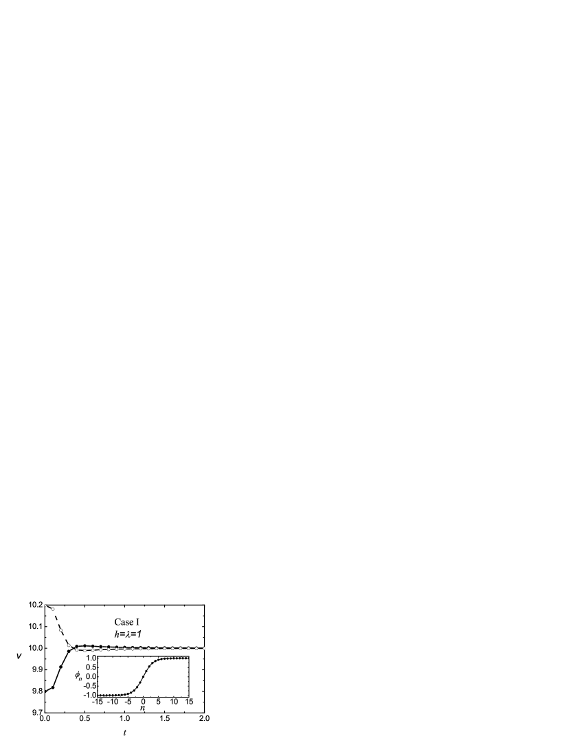
Figure 2: Kink velocity as a function of time for the Case I. The exact kink velocity for chosen model parameters is $v=10$ but for setting the initial conditions we put in Eq. (7) $v=9.8$ (dots) and $v=10.2$ (open circles). In both cases, regardless of the sign of perturbation, the kink velocity rapidly approaches the exact value. The inset shows the moving kink profile. Model parameters: $\lambda=h=1$, $A_{1}=-20$, $A_{4}\approx-222.1$, $A_{2}=\lambda-A_{1}-A_{4}$, $A_{3}=A_{5}=A_{6}=0$.

III Numerics

Let us analyze the kink solutions for the cases I and II described in Sec. II.2. Only the case of $\lambda=1$ will be analyzed.

In our simulations we solve the set of equations of motion, Eq. (I), numerically with a sufficiently small time step $\tau$ using the Stormer integration scheme of order $O(\tau^{6})$. Initial conditions are set by utilizing Eq. (7) with various parameters. Anti-periodic or fixed boundary conditions are employed.

III.1 Exact moving kinks in Case I

In this case, as it was already mentioned, the exact moving kink solution exists for the free model parameters satisfying $A_{1}\leq 0$ and $A_{4}\leq A_{1}-\lambda+2/h^{2}$ (see Fig. 1 where for $\lambda=h=1$ we show the isolines of equal kink velocity on the plane of model parameters $A_{1}$, $A_{4}$). On the line $A_{1}=0$, according to the first expression of Eq. (12), the kink velocity $v$ vanishes. On the line $A_{4}=A_{1}-\lambda+2/h^{2}$ the kink velocity also vanishes. This is so because, as it can be seen from the second expression of Eq. (12), on this line we have $T=1$, i.e. $\beta\rightarrow\infty$ and kink width vanishes. On the line $A_{4}=A_{1}-\lambda+2/h^{2}$ we also have $B=2/h^{2}$, which corresponds to vanishing of the width of the phonon spectrum given by Eq. (30).

The vacuum $\phi_{n}=\pm 1$ is stable, i.e. the spectrum Eq. (30) does not have imaginary frequencies, if $A_{4}<A_{1}+2/h^{2}$, i.e., it is stable in the whole region where the exact moving kink solution is defined.

As it was already mentioned, the kink propagation velocity is unlimited and from Fig. 1 one can see that $|A_{4}|$ increases for higher kink velocities while $A_{1}$ can have any negative value. For example, for $v=10$ the moving kink exists for $A_{1}<0$ and $A_{4}<-221.9$.

Let us now turn to the discussion of the stability of moving kinks.

Case of $\lambda=h=1$ and $v=10$.

Moving kink solutions are stable not in the whole range of parameters of their existence but for each studied value of propagation velocity we were able to find a range of parameters where the moving kink is stable in the sense that even a perturbed kink solution (with a reasonably large perturbation amplitude) in course of time tends to the exact solution (i.e., it is effectively “attractive”). The evolution of the kink velocity in such self-regulated kink dynamics is shown in Fig. 2 for a velocity as large as $v=10$ for $A_{1}=-20$ at $\lambda=h=1$. For this choice, we have from Eq. (12) $\beta\approx 0.316$, $A_{4}\approx-222.1$, $A_{2}\approx 243.1$. The moving kink profile is shown in the inset of Fig. 2. The perturbation was introduced into the initial conditions by setting in the exact solution of Eq. (7), a “wrong” propagation velocity, smaller or higher than the exact value $v=10$. It can be seen that in course of time the propagation velocity approaches the exact value regardless of the sign of perturbation. The increase of kink velocity launched with $v=9.8$ may look counterintuitive but one should keep in mind that moving kinks are the solutions to a non-Hamiltonian (open) system with the possibility to have energy exchange with the surroundings with gain or loss, depending on the trajectories of particles (see, e.g., JPA2005 ).

We found that the absolutely stable, self-regulated motion of kink, similar to that shown in Fig. 2, for $v=10$ and $\lambda=h=1$ takes place within the range of $-164<A_{1}<-1.1$. The inverse kink width at the lower edge of the stability window is $\beta\approx 0.906$, which corresponds to a rather sharp kink, while for $A_{1}=-1.1$ (the upper edge of the stability window) one has $\beta\approx 0.0742$ and the kink is much wider than the lattice spacing $h$. For comparison, the kink shown in the inset of Fig. 2 has $\beta\approx 0.316$. For $A_{1}<-164$ the moving kink solution becomes unstable and displacements of particles behind the kink grow rapidly with time resulting in the stopping of numerical run due to floating point overflow. For $-1.1<A_{1}<0$ kink dynamics is as described in Sec. 6 of JPA2005 for the non-Hamiltonian case. In this region of parameter $A_{1}$, after a transition period, the kink starts to excite in the vacuum in its wake a wave with constant amplitude. In this regime, the kink attains a constant velocity whose value is, generally speaking, different from that prescribed by Eq. (12). Kink dynamics in the two unstable regimes described above will be illustrated below for the kinks moving with $v<1$.

Case of $\lambda=h=1$ and $v<1$.

Similar results were obtained for the kinks moving with small velocities ($v<1$). For smaller velocities the range of $A_{1}$ with stable, self-regulated motion becomes narrower. For instance, a kink with $v=0.8$ is stable (in the above mentioned sense) for $-2.4<A_{1}<-0.10$, while the one with $v=0.5$ for $-0.19<A_{1}<-0.06$.

In Fig. 3 we show the time variation of the moving kink profile to demonstrate the instability of the exact kink solution moving with $v=0.8$ at $A_{1}=-2.6$. This solution is unstable and, due to the presence of rounding error perturbation, the wave behind the kink is excited. The amplitude of the wave rapidly grows with time and it becomes noticeable in the scale of the figure at $t>100$. At $t\approx 130$ the numerical run stops due to the floating point overflow. Kink velocity is nearly equal to $v=0.8$ practically until the collapse of the wave behind it.

In Fig. 4 we show the kink velocity as a function of time to illustrate the instability of the exact moving kink solution at $v=0.8$ and $A_{1}=-0.07$. This solution is unstable and, due to the presence of rounding error perturbation, at $t\approx 400$ it starts to transform into an oscillating kink (with the period $T\approx 5.01$) moving with different velocity and exciting a constant-amplitude wave behind it. The transformation is essentially complete by $t\approx 5000$ and the kink velocity becomes $v\approx 0.96$. The inset shows the profiles of an oscillating moving kink in the two configurations with the most deviation from the average in time configuration.

Case of $\lambda=1$, $h=0.1$, and $v=10$.

Stable, self-regulated motion of high-speed kinks was also observed for as small lattice spacing as $h=0.1$. This may appear surprising at first sight because for small $h$ one would expect the discrete model to be close to the continuum $\phi^{4}$ model where propagation with the velocity faster than $v=1$ is impossible. But looking at Eq. (26), one can notice that the two last non-Lorentz-invariant terms have the coefficients $h^{2}B$ and $h^{2}D$, and they are not small even for small $h$ if $B$ and $D$ are large. The high-speed kink in the considered case indeed exists for $B\approx-19833.1$ and $D\approx 20034.1$. These values correspond to the following parameters considered in this numerical run: $A_{1}=-200.0$, $A_{4}\approx-20034.1$, $A_{2}=\lambda-A_{1}-A_{4}\approx 20235.1$, $A_{3}=A_{5}=A_{6}=0$, $\beta=1$.

Figure 3: Change of the moving kink profile demonstrating the instability of the exact solution for the following set of model parameters: $\lambda=h=1$, $A_{1}=-2.6$, $A_{4}\approx-2.538$, $A_{2}=\lambda-A_{1}-A_{4}\approx 6.138$, $A_{3}=A_{5}=A_{6}=0$. Exact kink parameters are $v=0.8$, $\beta\approx 1.425$. This solution is unstable and, due to the presence of rounding error perturbation, the wave behind the kink is excited. The amplitude of the wave rapidly growths with time and it becomes noticeable in the scale of the figure at $t>100$. At $t\approx 130$ the numerical run stops due to the floating point overflow.

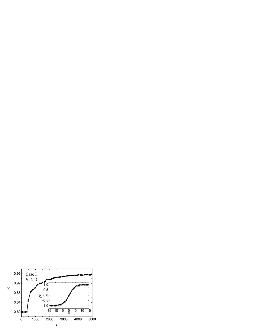
Figure 4: Kink velocity as a function of time demonstrating the instability of the exact moving kink solution for the following set of model parameters: $\lambda=h=1$, $A_{1}=-0.07$, $A_{4}\approx-18.28$, $A_{2}=\lambda-A_{1}-A_{4}\approx 19.35$, $A_{3}=A_{5}=A_{6}=0$. Exact kink parameters are $v=0.8$, $\beta\approx 0.234$. This solution is unstable and, due to the presence of rounding error perturbation, at $t\approx 400$ it starts to transform to an oscillating moving kink (with the period $T\approx 5.01$). The transformation is essentially complete by $t\approx 5000$. Inset shows the profiles of the oscillating moving kink in the two configurations with the most deviation from the average in time configuration.

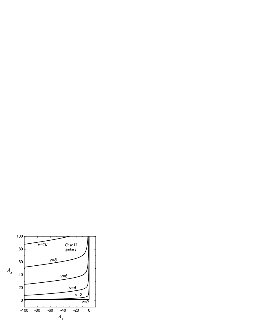
Figure 5: Isolines of equal kink velocity on the plane of model parameters $A_{1}$, $A_{4}$ at $\lambda=h=1$ for the case II when model parameters satisfy Eq. (II.2).

III.2 Exact moving kinks in Case II

In the case II, the model parameters are related by Eq. (II.2) and we find $B=-2A_{4}+6/h^{2}$. As it was already mentioned, the exact moving kink solution exists for $A_{1}<0$ and $A_{4}>2/h^{2}$. Isolines of equal kink velocity on the plane of the free model parameters $A_{1}$, $A_{4}$ can be seen in Fig. 5 for $\lambda=h=1$. In the Case II, similarly to the Case I, on the borders of the existence of the kink solution the kink velocity vanishes. Moreover, on the border $A_{4}=2/h^{2}$, both the width of the phonon spectrum given by Eq. (30) and the kink width vanish, and this is also similar to what we saw in Case I.

As was mentioned above, the exact moving kink solution in the Case II can also have arbitrary velocity. Kink dynamics in the Case II was observed to be qualitatively similar to that of the Case I. For the kink with speed as large as $v=10$ for $\lambda=h=1$ we found that the absolutely stable self-regulated motion is observed within the range of $-82<A_{1}<-1.0$. The corresponding inverse kink width varies in the range $0.640<\beta<0.0707$. For $A_{1}<-82$ the moving kink solution becomes unstable and displacements of particles in the wake of the kink grow rapidly with time resulting in the termination of numerical run due to floating point overflow. For $-1.0<A_{1}<0$, after a transition period, the kink starts to excite in the vacuum behind itself a wave with constant amplitude. In this regime, the kink propagates with a constant velocity whose value is, generally speaking, different from that prescribed by Eq. (15).

III.3 Exact moving four-periodic solution

We have studied the dynamics of the exact moving four-site periodic solution Eq. (23) in the Hamiltonian model, i.e., with the parameters satisfying Eq. (25). Periodic boundary conditions were employed for a chain of 40 particles. A small perturbation was introduced in the amplitude of particles at $t=0$ and we always observed a growth of deviation of the perturbed solution away from the exact one. We varied the free model parameter $\gamma_{1}$ and the solution parameter $v$ in wide ranges at $\lambda=h=1$ but could not find a stable regime.

IV Conclusions

For the discrete model of Eq. (I), in Sec. II.1 we obtained exact moving solutions in the form of the sn Jacobi elliptic function. Solutions in the form of cn and dn Jacobi elliptic functions can also be constructed as well as the solutions having the form of 1/sn, 1/cn, and sndn/cn in analogy with DKKS2007_BOP . In Sec. II.2, from the sn solution, in the limit of $m\rightarrow 1$, we extracted the exact moving kink solution in the form of tanh, i.e., the corresponding hyperbolic function solution.

Setting $v=0$ in the exact moving solutions obtained in this work one obtains the TI static solutions reported in ArXivKDS . In this sense, the results reported here generalize our previous results. We thus reveal the hidden connection between the static TI solutions and the exact moving solutions. Such solutions can be derived from a three-point map reducible to a two-point map (see Sec. II.6) i.e., from an integrable map Quispel .

We have demonstrated that the exact moving solutions to lattice and continuous equations with competing nonlinear terms can have any large propagation velocity. Most of the high-speed solutions reported in the present study are solutions to the non-Hamiltonian variant of the considered $\phi^{4}$ models. However, the trigonometric solution described in Sec. II.3 exists also in the Hamiltonian lattice and it also can have an arbitrary speed.

While the problem of identifying traveling solutions in the one-dimensional context by now has a considerable literature associated with it, as evidenced above, identifying such solutions in higher dimensional problems is to a large extent an open question. While initial studies have demonstrated the possibility in some of these systems for traveling in both on- and off-lattice directions susanto , analytical results along the lines discussed here are essentially absent in that problem and could certainly assist in clarifying the potential of coherent structures for unhindered propagation in these higher dimensional settings.

References

- (1) E. Infeld and G. Rowlands, Nonlinear Waves, Solitons and Chaos, Cambridge University Press (Cambridge, 2000)
- (2) T. Dauxois and M. Peyrard, Physics of Solitons, Cambridge University Press (Cambridge, 2006).
- (3) M. Toda, Theory of Nonlinear Lattices (Springer-Verlag, Berlin, 1981).
- (4) M. J. Ablowitz and J. F. Ladik, J. Math. Phys. 16, 598 (1975); M. J. Ablowitz and J. F. Ladik, J. Math. Phys. 17, 1011 (1976).
- (5) S. J. Orfanidis, Phys. Rev. D 18, 3828 (1978).
- (6) Encyclopedia of Nonlinear Science, Edited by A. Scott (Routledge, New York, 2005).
- (7) P. G. Kevrekidis, Physica D 183, 68 (2003).
- (8) J. M. Speight and R. S. Ward, Nonlinearity 7, 475 (1994); J. M. Speight, Nonlinearity 10, 1615 (1997); J. M. Speight, Nonlinearity 12, 1373 (1999).
- (9) C. M. Bender and A. Tovbis, J. Math. Phys. 38, 3700 (1997).
- (10) S. V. Dmitriev, P. G. Kevrekidis, and N. Yoshikawa, J. Phys. A 38, 1 (2005).
- (11) F. Cooper, A. Khare, B. Mihaila, and A. Saxena, Phys. Rev. E 72, 36605 (2005).
- (12) I. V. Barashenkov, O. F. Oxtoby, and D. E. Pelinovsky, Phys. Rev. E 72, 35602R (2005).
- (13) S. V. Dmitriev, P. G. Kevrekidis, and N. Yoshikawa, J. Phys. A 39, 7217 (2006).
- (14) O.F. Oxtoby, D.E. Pelinovsky, and I.V. Barashenkov, Nonlinearity 19, 217 (2006).
- (15) S. V. Dmitriev, P. G. Kevrekidis, N. Yoshikawa, and D. J. Frantzeskakis, Phys. Rev. E 74, 046609 (2006).
- (16) J. M. Speight and Y. Zolotaryuk, Nonlinearity 19, 1365 (2006).
- (17) S. V. Dmitriev, P. G. Kevrekidis, A. Khare, and A. Saxena, J. Math. Phys. 40, 6267 (2007).
- (18) I. Roy, S. V. Dmitriev, P. G. Kevrekidis, and A. Saxena, Phys. Rev. E 76, 026601 (2007).
- (19) A. Khare, S. V. Dmitriev, A. Saxena, Exact Static Solutions of a Generalized Discrete Model Including Short-Periodic Solutions, arXiv:0710.1460.
- (20) S.V. Dmitriev, P.G. Kevrekidis, A.A. Sukhorukov, N. Yoshikawa, and S. Takeno, Phys. Lett. A 356, 324 (2006).
- (21) S. V. Dmitriev, P. G. Kevrekidis, N. Yoshikawa, and D. Frantzeskakis, J. Phys. A 40, 1727 (2007).
- (22) A. Khare, S. V. Dmitriev, and A. Saxena, J. Phys. A 40, 11301 (2007).
- (23) A. Khare, K.O. Rasmussen, M.R. Samuelsen, A. Saxena, J. Phys. A 38, 807 (2005); A. Khare, K.O. Rasmussen, M. Salerno, M.R. Samuelsen, and A. Saxena, Phys. Rev. E 74, 016607 (2006).
- (24) D.E. Pelinovsky, Nonlinearity 19, 2695 (2006).
- (25) P.G. Kevrekidis, S.V. Dmitriev, and A.A. Sukhorukov, Math. Comput. Simulat. 74, 343 (2007).
- (26) A.A. Aigner, A.R. Champneys, and V.M. Rothos, Physica D 186, 148 (2003).
- (27) T. R. Melvin, A. R. Champneys, P. G. Kevrekidis, and J. Cuevas, Phys. Rev. Lett. 97, 124101 (2006); T.R.O. Melvin, A.R. Champneys, P.G. Kevrekidis, and J. Cuevas, Physica D, in press (2008).
- (28) G. Iooss and D.E. Pelinovsky, Physica D 216, 327 (2006).
- (29) D.E. Pelinovsky and V.M. Rothos, Physica D 202, 16 (2005).
- (30) O. F. Oxtoby and I. V. Barashenkov, Phys. Rev. E 76, 036603 (2007).
- (31) I. V. Barashenkov, O. F. Oxtoby, and D. E. Pelinovsky, Phys. Rev. E 72, 035602 (2005).
- (32) O. F. Oxtoby, D. E. Pelinovsky, and I. V. Barashenkov, Nonlinearity 19, 217 (2006).
- (33) L. Hadžievski, A. Maluckov, M. Stepić, and D. Kip, Phys. Rev. Lett. 93, 033901 (2004); M. Stepić, D. Kip, L. Hadžievski, and A. Maluckov, Phys. Rev E 69 (2004) 066618;
- (34) A. Maluckov, L. Hadžievski, and M. Stepić, Physica D 216, 95 (2006).
- (35) S. Flach, Y. Zolotaryuk, and K. Kladko, Phys. Rev. E 59, 6105 (1999).
- (36) G.P. Tsironis, J. Phys. A 35, 951 (2002).
- (37) G.R.W. Quispel, J.A.G. Roberts, and C.J. Thompson, Physica D 34, 183 (1989).
- (38) H. Susanto, P.G. Kevrekidis, R. Carretero-González, B.A. Malomed, and D.J. Frantzeskakis, Phys. Rev. Lett. 99, 214103 (2007).