1 Threshold resummation

In describing a charged particle-antiparticle system near threshold, it is well known from QED that the so-called Coulomb resummation factor plays an important role. This resummation, performed on the basis of the nonrelativistic Schrödinger equation with the Coulomb potential $V(r)=-\alpha/r$, leads to the Sommerfeld-Sakharov $S$-factor [1]. In the threshold region one cannot truncate the perturbative series and the $S$-factor should be taken into account in its entirety. The $S$-factor appears in the parametrization of the imaginary part of the quark current correlator, which can be approximated by the Bethe-Salpeter amplitude of the two charged particles, $\chi_{\rm{BS}}(x=0)$ [2]. The nonrelativistic replacement of this amplitude by the wave function, which obeys the Schrödinger equation with the Coulomb potential, leads to the appearance of the resummation factor in the parametrization of the normalized $e^{+}e^{-}$ to hadrons cross section ratio $R(s)$.

For a systematic relativistic analysis of quark-antiquark systems, it is essential from the very beginning to have a relativistic generalization of the $S$-factor. A new form for this relativistic factor in the case of QCD was proposed by Solovtsov in 2001 [3].

$$S(\chi)=\frac{X(\chi)}{1-\exp\left[-X(\chi)\right]}\,,\quad\quad X(\chi)=\frac{\pi\,\alpha}{\sinh\chi}\,,$$ (1)

where $\chi$ is the rapidity which is related to $s$ by $2m\cosh\chi=\sqrt{s}$, $\alpha\to 4\alpha_{s}/3$ in QCD. The function $X(\chi)$ can be expressed in terms of $v=\sqrt{1-4m^{2}/s}$: $X(\chi)=\pi\alpha\sqrt{1-v^{2}}/v$. The relativistic resummation factor (1) reproduces both the expected nonrelativistic and ultrarelativistic limits and corresponds to a QCD-like Coulomb potential. Here we consider the vector channel for which a threshold resummation $S$-factor for the s-wave states is used. For the axial-vector channel the $P$-factor is required. The corresponding relativistic factor has been found recently [4].

To incorporate the quark mass effects one usually uses the approximate expression above the quark-antiquark threshold [5]

$${\cal{R}}(s)=T(v)\,\left[1+g(v)r(s)\right]\,,$$ (2)

where

$$T(v)=v\frac{3-v^{2}}{2}\,,\quad g(v)=\frac{4\pi}{3}\left[\frac{\pi}{2v}-\frac{3+v}{4}\left(\frac{\pi}{2}-\frac{3}{4\pi}\right)\right]\,.$$ (3)

The function $g(v)$ is taken in the Schwinger approximation [1].

One cannot directly use the perturbative expression for $r(s)$ in Eq. (2), which contains unphysical singularities, to calculate, for example, the Adler $D$-function. Instead, one can use the analytic perturbation theory (APT) representation for $r(s)$. The explicit three-loop form for $r_{\rm APT}(s)$ can be found in Ref. [6]. Besides this replacement, one has to modify the expression (2) in such a way as to take into account summation of an arbitrary number of threshold singularities. Including the threshold resummation factor (1) leads to the following modification of the expression (2) for a particular quark flavor $f$ [6, 7]

$${\cal{R}}_{f}(s) = \left[R_{0,f}(s)+R_{1,f}(s)\right]\Theta(s-4m_{f}^{2}),$$ (4)

$$R_{0}(s) = T(v)\,S(\chi),\qquad R_{1}(s)=T(v)\left[\,r_{\rm{APT}}(s)\,g(v)-\frac{1}{2}X(\chi)\,\right].$$

The usage of the resummation factor (1) reflects the assumption that the coupling is taken in the $V$ renormalization scheme. To avoid double counting, the function $R_{1}$ contains the subtraction of $X(\chi)$. The potential term corresponding to the $R_{0}$ function gives the principal contribution to ${\cal{R}}(s)$, as shown in Fig. 1, the correction $R_{1}$ amounting to less than twenty percent over the whole energy interval. For a recent account of some of the successes of APT including Coulomb resummation see Ref. [8].

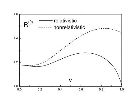
Fig. 1: Behavior of $R_{0}(s)$ with relativistic and nonrelativistic $S$-factors.

2 Dirac Magnetic Monopoles

The relativistic interaction between an electric and a magnetic current is [9]

$$W(j,{}^{*}j)=\int(dx)(dx^{\prime})(dx^{\prime\prime}){}^{*}j^{\mu}(x)\epsilon_{\mu\nu\sigma\tau}\partial^{\nu}f^{\sigma}\left(x-x^{\prime}\right)D_{+}\left(x^{\prime}-x^{\prime\prime}\right)j^{\tau}\left(x^{\prime\prime}\right).$$ (5)

Here the electric and magnetic currents are

$$j_{\mu}=e\bar{\psi}\gamma_{\mu}\psi\qquad\mbox{and}\qquad{}^{*}j_{\mu}=g\bar{\chi}\gamma_{\mu}\chi,$$ (6)

for example, for spin-1/2 particles. The photon propagator is denoted by $D_{+}(x-x^{\prime})$ and $f_{\mu}(x)$ is the Dirac string function which satisfies the differential equation

$$\partial_{\mu}f^{\mu}(x)=4\pi\delta(x).$$ (7)

A formal solution of this equation is given by

$$f^{\mu}(x)=4\pi n^{\mu}\left(n\cdot\partial\right)^{-1}\delta(x),$$ (8)

where $n^{\mu}$ is an arbitrary constant vector.

Dirac showed in 1931 [10] that quantum mechanics was consistent with the existence of magnetic monopoles provided the quantization condition holds,

$$eg=m^{\prime}\hbar c,$$ (9)

where $m^{\prime}$ is an integer or an integer plus 1/2, which explains the quantization of electric charge. This was generalized by Schwinger to dyons, particles carrying both electric charge $e_{a}$ and magnetic charge $g_{a}$ [11]:

$$e_{1}g_{2}-e_{2}g_{1}=-m^{\prime}\hbar c.$$ (10)

(Schwinger sometimes argued that $m^{\prime}$ was an integer, or perhaps an even integer.) For details on the derivation of these quantization conditions, see, for example, Ref. [9]. In the following we write $m^{\prime}=n/2.$

3 OU Monopole Experiment: Fermilab E882

We now refer to the experiment conducted at the University of Oklahoma from 1997–2004 [12], searching for low-mass monopoles which might have been produced at the Tevatron and captured in the old CDF and D0 detectors.

The best prior experimental limit on the direct accelerator production of magnetic monopoles is that of Bertani et al. in 1990 [13]

$$\sigma\leq 2\times 10^{-34}\mbox{cm}^{2}\quad\mbox{for a monopole mass}\quad M\leq 850\,\mbox{GeV}.$$ (11)

(Such limits are complementary to searches for cosmic “intermediate mass” magnetic monopoles, with masses between $10^{5}$ and $10^{12}$ GeV, such as have been recently reported in Ref. [14].) We are able to set much better limits than Bertani et al. because the integrated luminosity is $10^{4}$ times that of the previous 1990 experiment:

$$\int{\cal L}=172\pm 8\,\mbox{pb}^{-1}\quad(\mbox{D0}).$$ (12)

The fundamental mechanism is supposed to be a Drell-Yan process,

$$p+\bar{p}\to q+\bar{q}+X\to M+\bar{M}+X,$$ (13)

where the cross section is given by

$$\frac{d\sigma}{d\mathcal{M}}=(68.5n)^{2}\beta^{3}\frac{8\pi\alpha^{2}}{9s}\int\frac{dx_{1}}{x_{1}}\sum_{i}Q_{i}^{2}q_{i}(x_{1})\bar{q}_{i}\left(\frac{\mathcal{M}^{2}}{sx_{1}}\right).$$ (14)

Here $\mathcal{M}$ is the invariant mass of the monopole-antimonopole pair, and we have included a factor of $\beta^{3}$ to reflect both phase space and the velocity suppression of the magnetic coupling, as roughly implied by Eq. (5).

Any monopole produced at the Tevatron is trapped in the detector elements with 100% probability due to interaction with the magnetic moments of the nuclei, based on the theory described in my review [9]. The experiment consists of running samples obtained from the old D0 and CDF detectors through a superconducting induction detector. Figure 2 is a sketch of the D0 detector.

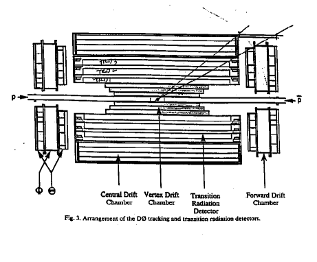
Fig. 2: Arrangement of the D0 tracking and transition radiation detectors.

We use energy loss formula of Ahlen [15] to describe the interaction of the monopoles with the detector elements.

Figure 3 is a diagram of the OU magnetic monopole induction detector. It is a cylindrical detector, with a warm bore of diameter 10 cm, surrounded by a cylindrical liquid N₂ dewar, which insulated a liquid He dewar. The superconducting loop detectors were within the latter, concentric with the warm bore. Any current established in the loops was detected by a SQUID. The entire system was mechanically isolated from the building, and magnetically isolated by $\mu$ metal and superconducting lead shields. The magnetic field within the bore was reduced with the help of Helmholtz coils to about 1% of the earth’s field. Samples were pulled vertically through the warm bore with a computer-controlled stepper motor. Each traversal took about 50 s; every sample run consisted of some 20 up and down traversals. Most samples were run more than once, and more than 660 samples of Be, Pb, and Al from both the old CDF and D0 detectors were analyzed over a period of 7 years.

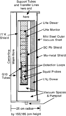
Fig. 3: Sketch of the OU induction detector. Shown is a vertical cross section; it should be imagined as rotated about the vertical axis labelled “centerline.”

A monopole passing through the superconducting loop would produce a step in the current

$$LI=\frac{4\pi g}{c}-\frac{\Delta\Phi}{c}=\frac{4\pi g}{c}\left(1-\frac{r^{2}}{a^{2}}\right).$$ (15)

where $L$ is the inductance of the loop, $r$ is the radius of the loop, and $a$ is the radius of the superconducting cylinder. The detector was calibrated with a pseudopole, a long solenoid, and the resulting steps in the output of the SQUID are seen in Fig. 4 to agree with theory.

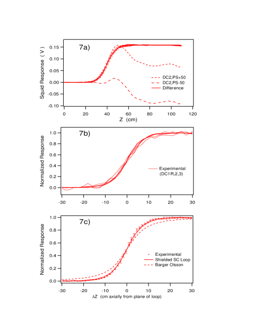
Fig. 4: Typical step plots: D0 aluminum, CDF lead, and CDF aluminum. The experimental data was collected from pseudopole simulations; the steps shown are for the difference between the results with reversed polarizations of the pseudopole. Data agrees well with the SC theory, which incorporates the effect of the shielded superconducting loops. The theory without the shield, given by Barger and Ollson [16] is also shown.

Figure 5 shows the histogram of steps from data collected from D0 samples. Similar histograms were obtained from the CDF data.

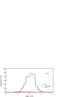
Fig. 5: Steps from D0 samples. A Dirac pole would appear as a step at 2.46 mV.

From this, we can obtain limits on cross sections for the production of monopole–antimonopole pairs, and then, model dependent limits on monopole masses, as shown in Fig. 6.

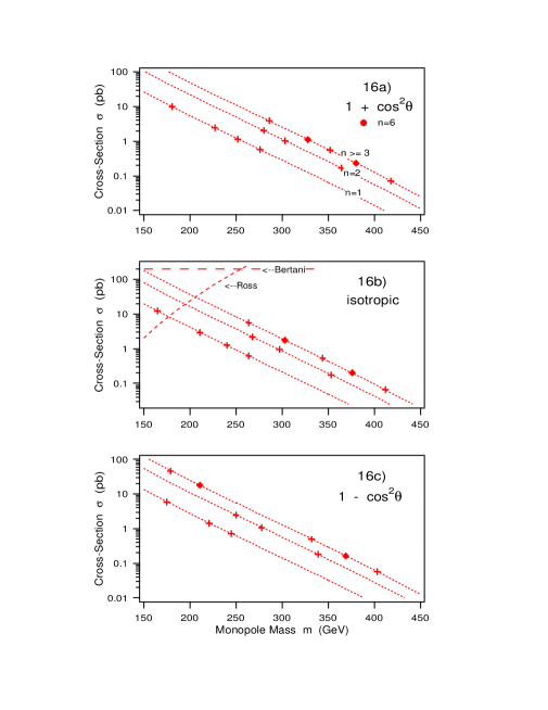
Fig. 6: Cross section vs. mass limits. The three graphs show three different assumptions about the angular distribution, since even if we knew the spin of the monopole, we cannot at present predict the differential cross section. Shown in the second figure are the Bertani (1990) [13] and lunar (1973) [17] limits.

Table 1: Alternative interpretations for different production angular distributions of the monopoles, comparing $1$ and $1\pm\cos^{2}\theta$ (90% CL). Here the upper cross section limits $\sigma_{a}$ corresponds to the distribution $1+a\cos^{2}\theta$, and similarly for the lower mass limits $\mu$ (all at 90% confidence level).

Set	$2m^{\prime}$	$\sigma_{+1}$	$\mu_{+1}$	$\sigma_{0}$	$\mu_{0}$	$\sigma_{-1}$	$\mu_{-1}$
		(pb)	(GeV/$c^{2}$)	(pb)	(GeV/$c^{2}$)	(pb)	(GeV/$c^{2}$)
1 Al	1	1.2	250	1.2	240	1.4	220
1 Al RM	1	0.6	275	0.6	265	0.7	245
2 Pb	1	9.9	180	12	165	23	135
2 Pb RM	1	2.4	225	2.9	210	5.9	175
1 Al	2	2.1	280	2.2	270	2.5	250
2 Pb	2	1.0	305	0.9	295	1.1	280
3 Al	2	0.2	365	0.2	355	0.2	340
1 Be	3	3.9	285	5.6	265	47	180
2 Pb	3	0.5	350	0.5	345	0.5	330
3 Al	3	0.07	420	0.07	410	0.06	405
1 Be	6	1.1	330	1.7	305	18	210
3 Al	6	0.2	380	0.2	375	0.2	370

Table 1 shows the limits we obtained for different sample sets, and different charges $m^{\prime}$, for various assumed production distributions. Our best mass limits are (assuming isotropic distribution)

• $m^{\prime}=\frac{1}{2}$: $\mu>265$ GeV

• $m^{\prime}=1$: $\mu>355$ GeV

• $m^{\prime}=\frac{3}{2}$: $\mu>410$ GeV

• $m^{\prime}=3$: $\mu>375$ GeV.

4 Reanalysis of Monopole Mass Limits Using Coulomb Resummation

We will now use the Solovtsov Coulomb threshold correction (4) in the form

$$R=T(v)[S(\chi)-\frac{1}{2}X(\chi)],$$ (16)

with $T(v)$ given in (3) and $S(\chi)$ given in (1), or

$$X(\chi)=\pi\alpha\frac{\sqrt{1-v^{2}}}{v},\quad S(\chi)=\frac{X(\chi)}{1-e^{-X(\chi)}}.$$ (17)

We have simply neglected the perturbative term, as uncalculable.

This is a small correction in QED, but here from Eq. (9)

$$\alpha\to 137\left(\frac{n}{2}\right)^{2},\quad n=1,2,3,\dots.$$ (18)

Figure 7 shows the substantial resulting increase in the cross section. This essentially pushes the cross section to the unitarity limit,

$$\sigma\leq\frac{\pi(2J+1)}{s}\sim\frac{3\pi}{s}.$$ (19)

As a result, for all charge states, our limits become

$$\mu>400\,\mbox{GeV}.$$ (20)

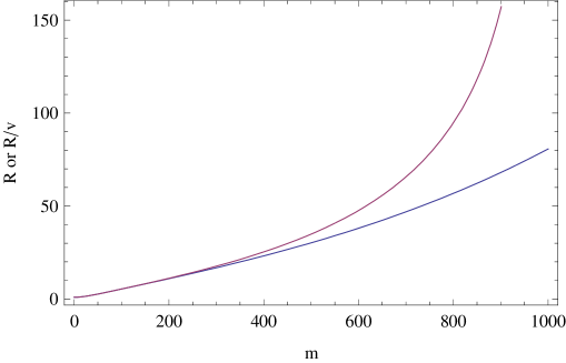
Fig. 7: Enhancement factor $R$ for the theoretical monopole cross section due to Coulomb resummation, as a function of monopole mass $\mu=\frac{\mathcal{M}}{2}m$, where $\mathcal{M}$ is the invariant mass of the monopole-antimonopole pair in TeV, and $\mu$ and $m$ are in GeV. The bottom curve shows $R$ given in Eq. (16), while in the top curve this factor is divided by the monopole velocity, since that is already included in the analysis, see Eq. (14).

5 Conclusions

The relativistic Coulomb resummation factor plays an important role in analysis of QCD experiments. Because the coupling is strong, it also plays a significant role in the theory of the production of magnetic monopole–anti-monopole pairs. Of course, because of the strong coupling, and even more because of the nonperturbative aspects of the Dirac string, there are potentially other effects which are just as strong but uncalculable. Our estimates of production rates were therefore extremely conservative, and a realistic assessment of the situation suggests that the limits on monopole masses from the Oklahoma experiment are at least as strong as the published limit from the very different CDF experiment [18]:

$$\mu_{\rm CDF}\geq 360\,\mbox{GeV},$$ (21)

References

- [1] A. Sommerfeld, Atombau and Spektallinien, vol. 2 (Vieweg, 1939); A. D. Sakharov, Zh. Eksp. Teor. Fiz. 18, 631 (1948); J. Schwinger, Particles, Sources, and Fields, vol. 2 (Addison-Wesley, 1973, Perseus, 1998).
- [2] R. Barbieri, P. Christillin, and E. Remiddi, Phys. Rev. D 8, 2266 (1973).
- [3] K. A. Milton and I. L. Solovtsov, Mod. Phys. Lett. A 16, 2213 (2001)
- [4] I. L. Solovtsov, O. P. Solovtsova, and Yu. D. Chernichenko, Phys. Part. Nucl. Lett. 2, 199 (2005).
- [5] E. C. Poggio, H. R. Quinn, and S. Weinberg, Phys. Rev. D 13, 1958 (1976); T. Appelquist and H. D. Politzer, Phys. Rev. Lett. 34, 43 (1975); Phys. Rev. D 12, 1404 (1975).
- [6] K. A. Milton, I. L. Solovtsov, and O. P. Solovtsova, Phys. Rev. D 64, 016005 (2001).
- [7] A. N. Sissakian, I. L. Solovtsov, and O. P. Solovtsova, JETP Lett. 73, 166 (2001).
- [8] K. A. Milton, I. L. Solovtsov and O. P. Solovtsova, Mod. Phys. Lett. A 21, 1355 (2006) [arXiv:hep-ph/0512209].
- [9] K. A. Milton, Rep. Prog. Phys. 69, 1637 (2006).
- [10] P. A. M. Dirac, Proc. R. Soc. London A 133, 60 (1931).
- [11] J. Schwinger, Science 165, 757 (1969).
- [12] Kalbfleisch et al., Phys. Rev. Lett. 85, 5292 (2000); Phys. Rev. D 69, 052002 (2004).
- [13] M. Bertani et al., Europhys. Lett. 12, 613 (1990).
- [14] S. Balestra et al., arXiv:0801.4913 [hep-ex].
- [15] S. P. Ahlen and K. Kinoshita, Phys. Rev. D 26, 2347 (1982); S. P. Ahlen, in Magnetic Monopoles, ed. R. A. Carrigan and W. P. Trower (New York, Plenum, 1982), p. 259.
- [16] V. Barger and M. G. Ollson, Classical Electricity and Magnetism (Boston: Allyn and Bacon, 1967).
- [17] R. R. Ross, P. H. Eberhard, L. W. Alvarez, and R. D. Watt, Phys. Rev. D 8, 698 (1973).
- [18] A. Abulencia et al. [CDF Collaboration], Phys. Rev. Lett. 96, 201801 (2006) [arXiv:hep-ex/0509015].