Mean-field dynamics of a Bose Josephson junction in an optical cavity

Abstract

We study the mean-field dynamics of a Bose Josephson junction which is dispersively coupled to a single mode of a high-finesse optical cavity. An effective classical Hamiltonian for the Bose Josephson junction is derived and its dynamics is studied in the perspective of phase portrait. It is shown that the strong condensate-field coupling does alter the dynamics of the Bose Josephson junction drastically. The possibility of coherent manipulating and in situ observation of the dynamics of the Bose Josephson junction is discussed.

Cavity quantum electrodynamics has now grown into a paradigm in the study of matter-field interaction. To tailor the atom-field coupling effectively, high degree of control over the center-of-mass motion of the atoms are essential. Although previous works have focused on the few-atom level kimble ; rempe ; chapman2 , recently, a great step was made as two groups succeeded independently in coupling a Bose-Einstein condensate to a single cavity mode esslinger ; colombe . That is, a single cavity mode dressed condensate has been achieved. This opens up a new regime in both the fields of cavity quantum electrodynamics and ultracold atom physics. In the condensate, all the atoms occupy the same motional mode, and couple identically to the cavity mode, thus realizing the Dicke model dicke in a broad sense. As shown by these experiments, the condensate is quite robust, it would not be destroyed by its interaction with the cavity mode.

In this paper, we investigate the mean-field dynamics of a Bose Josephson junction (BJJ), which is coupled to a driven cavity mode. This extends our previous work to the many-atom case zhang . The system may be constructed by splitting a Bose Einstein condensate, which already couples to a single cavity mode, into two weakly linked condensates, as can be done in various ways hofferberth ; levy ; schumm ; albiez ; shin . We restrict to the large detuning and low excitation limit, so that the atomic spontaneous emission can be neglected. In this limit, the effect of the strong coupling between the atoms and the field, seen by the field, is to shift the cavity resonance frequency and hence modifies the field intensity. Unlike the single condensate case, we now have two, which may couple with different strengths to the cavity mode because of the position dependence of the atom-field coupling. Consequently, the field dynamics is coupled to the tunneling dynamics of the BJJ, and vice versa. It is the interplay between the two sides that we are interested in. We would like to stress that, although there had been some experimental investigations on this subject and phenomena such as dispersive optical bistability were observed hemmerich ; gupta , all of them dealt with thermal cold atoms. However, here, the long coherence time of the condensates will surely make a difference.

The Hamiltonian of the system consists of three parts:

$$H=H_{a}+H_{f}+H_{\mathrm{int}}.$$ (1)

$H_{a}$ is the canonical Bose Josephson junction Hamiltonian in the two-mode approximation ($\hbar=1$ throughout),

$$H_{a}=-\Omega(b_{1}^{\dagger}b_{2}+b_{2}^{\dagger}b_{1})+\frac{V}{2}(b_{1}^{\dagger}b_{1}^{\dagger}b_{1}b_{1}+b_{2}^{\dagger}b_{2}^{\dagger}b_{2}b_{2}),$$ (2)

where $b_{1}^{\dagger}$, $b_{2}^{\dagger}$ ($b_{1}$, $b_{2}$) create (annihilate) an atom in its internal ground state in the left and right trap respectively. $\Omega$ is the tunneling matrix element between the two modes, while $V$ denotes the repulsive interaction strength between a pair of atoms in the same mode. The two-mode model assumes two stationary wave functions (the single-atom ground states actually) in the individual traps, while neglecting the modifications due to the atom-atom interaction. The regime in which this is the case can be found in Ref. walls . $H_{f}$ is the single-mode field Hamiltonian,

$$H_{f}=\omega_{c}a^{\dagger}a+\eta(t)e^{-i\omega_{p}t}a^{\dagger}+\eta^{\ast}(t)e^{i\omega_{p}t}a,$$ (3)

where $\omega_{c}$, $\omega_{p}$ are the cavity mode frequency and pump frequency respectively, and $\eta(t)$, the amplitude of the pump, varies slowly in the sense that $|\dot{\eta}/\eta|\ll\omega_{p}$. In the limit of large detuning detuning and weak pump, the atom field interaction is of dispersive nature, and the two-level atoms can be treated as scalar particles with the upper level being adiabatically eliminated. Under the two-mode approximation for the atoms, the interaction between the atoms and the cavity mode is ritsch1 ,

$$H_{\mathrm{int}}=U_{0}a^{\dagger}a(J_{1}n_{1}+J_{2}n_{2}),$$ (4)

where $U_{0}=g_{0}^{2}/(\omega_{c}-\omega_{a})$ is the light shift per photon, i.e. the potential per photon an atom feels at an antinode, $g_{0}$ being the atom-field coupling strength at an antinode. The two dimensionless parameters $J_{1,2}$ ($0\leq J_{1,2}\leq 1$) measure the overlaps between the atomic modes with the cavity mode zhang . $n_{1}=b_{1}^{\dagger}b_{1}$ ($n_{2}=b_{2}^{\dagger}b_{2}$) counts the atoms in the left (right) trap. The term $H_{\mathrm{int}}$ has a simple interpretation, from the point of view of the cavity mode, its frequency is renormalized; while from the point of view of the atom ensemble, the trapping potential is tilted provided $J_{1}\neq J_{2}$.

According to the Heisenberg’s equation, we have

$$i\dot{b_{1}} = -\Omega b_{2}+Vb_{1}^{\dagger}b_{1}b_{1}+J_{1}U_{0}a^{\dagger}ab_{1},$$ (5a)

$$i\dot{b_{2}} = -\Omega b_{1}+Vb_{2}^{\dagger}b_{2}b_{2}+J_{2}U_{0}a^{\dagger}ab_{2},$$ (5b)

$$i\dot{a} = \left[\omega_{c}+U_{0}(J_{1}n_{1}+J_{2}n_{2})\right]a-i\kappa a+\eta(t)e^{-i\omega_{p}t}.\quad$$ (5c)

Note that in Eq. (5c) we have put in the term $-i\kappa a$ to model the cavity loss, with $\kappa$ being the cavity loss rate. Under the mean-field approximation, we treat the operators $b_{1}$, $b_{2}$, and $a$ as classical quantities, $b_{1}\sim\sqrt{N_{1}}e^{i\theta_{1}}$, $b_{2}\sim\sqrt{N_{2}}e^{i\theta_{2}}$, $a\sim\alpha$. Here $N_{1}$, $N_{2}$ are respectively the numbers of atoms in the left and right condensates, and $\theta_{1}$, $\theta_{2}$ are their phases. By taking the mean field approximation, we actually confine to the so called Josephson regime as elaborated in detail in Ref. leggett . This regime is defined as $1/N\ll V/\Omega\ll N$, $N=N_{1}+N_{2}$ being the total atom number, and is characterized by small quantum fluctuations both in the relative phase $\phi\equiv\theta_{2}-\theta_{1}$ ($\Delta\phi\ll 1$) and in the populations $N_{1,2}$ ($\Delta N_{1,2}\ll\sqrt{N}$). This property then justifies the mean field approximation. As shown in Ref. smerzi3 , the mean field predictions (self-trapping etc.) are well recovered in a full quantum dynamics on a short time scale, and their breakdown occurs only at a long time scale which increases exponentially with the total atom number.

It is clear from Eq. (5c) that the relaxation time scale of the cavity mode is of order $1/\kappa$, which is much shorter than the plasma oscillation period of a bare Bose Josephson junction dressed which, roughly speaking, is of order $1/\Omega$. In fact, the typical values of $\kappa$ of high-finesse optical cavities are of order $2\pi\times 10^{6}$ Hz, while the experimentally observed $\Omega$ is of order $2\pi\times 10-2\pi\times 10^{2}$ Hz albiez . This implies that the cavity field follows the motion of the condensates adiabatically ritsch , thus from Eq. (5c) we solve

$$\langle a\rangle=\alpha(t)=\frac{\eta(t)e^{-i\omega_{p}t}}{i\kappa+[\omega_{p}-\omega_{c}-U_{0}(J_{1}N_{1}+J_{2}N_{2})]},$$ (6)

and the photon number is

$$\langle a^{\dagger}a\rangle=|\alpha(t)|^{2}=\frac{|\eta(t)|^{2}}{\kappa^{2}+[\Delta-\delta U_{0}(N_{1}-N_{2})/2]^{2}},$$ (7)

where $\Delta\equiv\omega_{p}-\omega_{c}-(J_{1}+J_{2})NU_{0}/2$, and $\delta\equiv J_{1}-J_{2}$ is the coupling difference between the two atomic modes to the cavity mode. We then see that with other parameters fixed, the photon number depends only on the atom population difference between the two traps. Moreover, the motion of the cavity mode couples to that of the condensates only in the case that the two traps are placed asymmetrically with respect to the cavity mode such that $\delta$ is nonzero. Considering that the cavity field intensity varies rapidly along the cavity axis (with period $\lambda/2\sim 0.5$ $\mu$m) while rather smoothly in the transverse plane (with mode waist $w\sim 10-25$ $\mu$m), and that the extension of the condensates and the separation between them are in between, it may be wise to create the coupling difference $\delta$ by transverse rather than longitudinal position difference between the two condensates. In the experiment of Colombe et al. colombe , the transverse position of the cigar-shaped condensate, which is aligned parallel to the cavity axis, can be adjusted in the full range of the cavity mode waist. On this basis, the condensate may be split along its long axis, by using of the radio-frequency-induced adiabatic potential hofferberth ; schumm , which is also compatible with an atom chip, into two parts offsetted in the transverse direction. For a mode waist $w=10$ $\mu$m, a separation $d=1$ $\mu$m is hopeful to create a coupling difference $\delta=0.12$ if the two condensates are located near the inflection point $x_{c}=w/2$ of the cavity field intensity.

By introducing the dimensionless parameter $z=(N_{1}-N_{2})/N$, which describes the population of the atoms between the two traps, we rewrite the photon number (7) as

$$|\alpha(z,t)|^{2}=\frac{A(t)^{2}}{(z-B)^{2}+C^{2}},$$ (8)

where the three dimensionless parameters are defined as $A(t)=\eta(t)/[\delta U_{0}N/2]$, $B=\Delta/[\delta U_{0}N/2]$, and $C=\kappa/[\delta U_{0}N/2]$. We may understand $A(t)$, $B$, and $C$ as the reduced pumping strength, reduced detuning, and reduced loss rate, respectively. Equation (8) implies that the photon number, as a function of $z$, is a Lorentzian centered at $z_{c}=B$ and with width $2C$. Since $-1\leq z\leq 1$, to maximize the influence of the condensates on the cavity field, it is desirable to have $B$ within the same interval and $C\lesssim 1$. Under these conditions, the atomic motion is able to shift the cavity in or out of resonance. Apart from the factor $\delta$, the latter condition means that, the light shift per photon times the number of atoms exceeds the resonance linewidth of the cavity, which has been realized both with a ring cavity hemmerich and with a Fabry-Perot cavity gupta .

In the following, we follow closely the line of Refs. smerzi ; smerzi2 . Substituting Eq. (8) into Eqs. (5a) and (5b), we find that the two equations can be rewritten in terms of $z$ and the phase difference $\phi$ as

$$\frac{dz}{dt} = -\sqrt{1-z^{2}}\sin\phi,$$ (9a)

$$\frac{d\phi}{dt} = \frac{z}{\sqrt{1-z^{2}}}\cos\phi+rz+\frac{\delta U_{0}}{2\Omega}|\alpha(z,t)|^{2},$$ (9b)

where the time has been rescaled in units of the Rabi oscillation time $1/(2\Omega)$, $2\Omega t\rightarrow t$. The dimensionless parameter $r\equiv NV/(2\Omega)>0$ measures the interaction strength against the tunneling strength. We further define a Hamiltonian $H_{c}=H_{c}(z,\phi,t)$ in which $z$ and $\phi$ are two conjugate variables, i.e., $\dot{z}=-\frac{\partial H_{c}}{\partial\phi}$, $\dot{\phi}=\frac{\partial H_{c}}{\partial z}$. Such a Hamiltonian is

$$H_{c}(z,\phi,t) = -\sqrt{1-z^{2}}\cos\phi+\frac{1}{2}rz^{2}+\frac{\delta U_{0}}{2\Omega}F(z,t),\quad\quad$$ (10)

$$F(z,t) = \frac{A(t)^{2}}{C}\arctan\left(\frac{z-B}{C}\right).$$ (11)

The first two terms in Eq. (10) are the Hamiltonian of a bare Bose Josephson junction as was first derived in Refs. smerzi ; smerzi2 . They describe the energy cost due to the phase twisting between the two condensates and the atom-atom repulsion respectively. The last term may be termed as a cavity field induced tilt, as can be seen from its derivation. It reflects that the two traps, which are originally symmetric, are now subjected to an offset determined by the atom populations. In its nature, this term is similar to the potential an atom feels when passing a cavity adiabatically haroche , with the variable $z$ playing the role of the center-of-mass of the atom. The Hamiltonian can be made explicitly time-dependent if the pump strength varies in time. This may offer us a tool to coherently manipulate the motion of a Bose Josephson junction chapman . However, in this work, we concentrate on the case that the pump strength is a constant, $\eta(t)\equiv\eta$, so that the system is autonomous and the Hamiltonian is conserved in time.

As a one degree-of-freedom Hamiltonian system and with the Hamiltonian itself being a first integral, the system is integrable and there is no chaos. The trajectory of the system in the phase space (plane) follows the manifold (line) of constant energy. Thus qualitatively speaking, the dynamics of the system is to a great extent determined by the structure of its phase portrait, or more specifically, the number of stationary points, their characters (minimum, maximum, or saddle), and their locations. Before proceeding forward, we have some remarks on the structure of the phase space of the system and its implications. Superficially, the Hamiltonian $H_{c}$ is defined on the rectangular domain, $-1\leq z\leq 1$, $0\leq\phi\leq 2\pi$. However, physically $\phi$ is periodic in $2\pi$, and for $z=\pm 1$, $\phi$ is not well defined, so we should identify $(z,0)$ with $(z,2\pi)$ and collapse the lines $(z=\pm 1,\phi)$ to two points [Mathematically, this is justified by the fact that $H_{c}(z,0)=H_{c}(z,2\pi)$, and $H_{c}(1,\phi)=C_{1}$, $H_{c}(-1,\phi)=C_{2}$, with $C_{1}$, $C_{2}$ being two constants]. Therefore, the domain of the Hamiltonian or the phase space of the system is homeomorphous to a sphere. The Euler’s theorem for a smooth function on a sphere states that the number of minima $m_{0}$, the number of saddles $m_{1}$, and that of maxima $m_{2}$, satisfy the relation $m_{0}-m_{1}+m_{2}=2$ euler . This relation can be checked in Fig. 1 below.

In the following, we explore the dynamics of a Bose Josephson junction uncoupled or coupled to a cavity mode in the perspective of phase portrait. This approach has the advantage that it captures the whole information of the BJJ dynamics into one Buonsante . As a first step, we work out the stationary points of the system, which are determined by the equations $\frac{\partial H_{c}}{\partial z}=0$, $\frac{\partial H_{c}}{\partial\phi}=0$. The second equation implies that $\phi=0$ or $\phi=\pi$. Substituting these two possible values of $\phi$ into the first one, we have two equations of $z$ respectively,

$$f_{1}(z)=rz+\frac{z}{\sqrt{1-z^{2}}}+\frac{\tilde{A}}{(z-B)^{2}+C^{2}} = 0,\quad$$ (12a)

$$f_{2}(z)=rz-\frac{z}{\sqrt{1-z^{2}}}+\frac{\tilde{A}}{(z-B)^{2}+C^{2}} = 0.\quad$$ (12b)

where $\tilde{A}=\delta U_{0}A^{2}/(2\Omega)$. The character (minimum, saddle, or maximum) of the possible stationary points are determined by the corresponding Hessian matrices.

As a benchmark, we first consider the uncoupled case. If $r<1$, there are a minimum $(z,\phi)=(0,0)$ and a maximum $(z,\phi)=(0,\pi)$. If $r>1$, the point $(z,\phi)=(0,0)$ keeps to be a minimum while $(z,\phi)=(0,\pi)$ turns now into a saddle point, and there are two maximum at $(z,\phi)=(\pm\sqrt{r^{2}-1}/r,\pi)$. The transition of the point $(z,\phi)=(0,\pi)$ from a maximum to a saddle, and the split (bifurcation) of this old maximum into two new maxima at $r=1$, mark the onset of running-phase and $\pi$-phase self-trapping states smerzi2 ; walls . Note that the aforementioned Euler’s theorem carries over from $r<1$ to $r>1$.

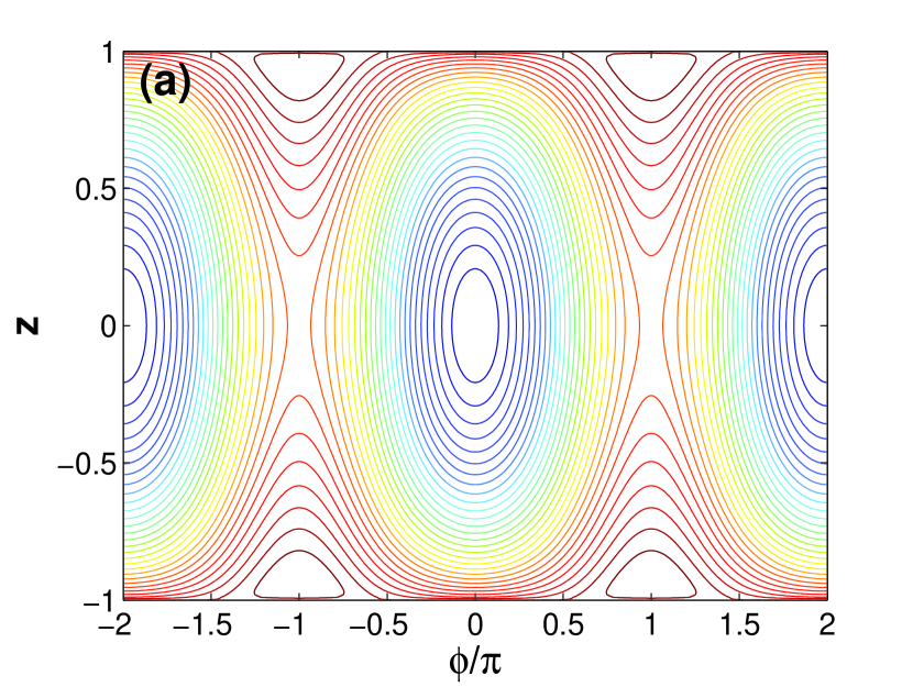
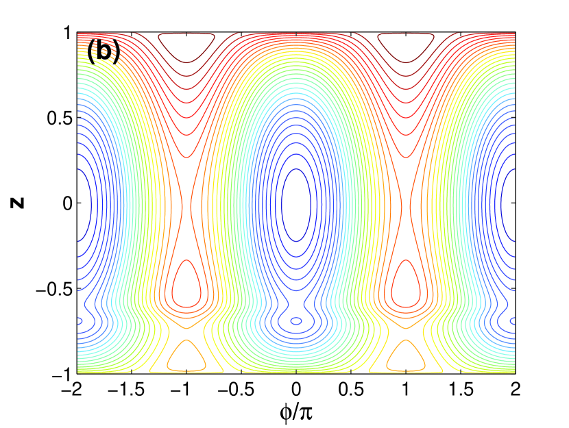
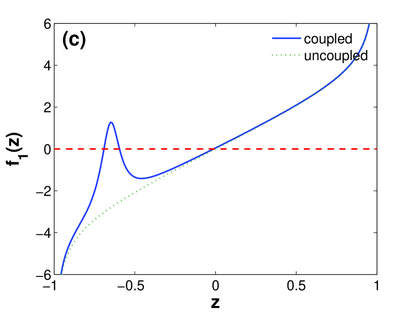
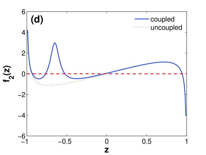
Figure 1: (Color online) Energy contours of a Bose Josephson junction (a) uncoupled and (b) coupled to a single cavity mode. (c) and (d): Gradient of the energy along the line $\phi=0$ and $\phi=\pi$, respectively. Zeros of $f_{1}(z)$ with positive (negative) derivatives correspond to minima (saddle points) of $H_{c}$, while zeros of $f_{2}(z)$ with positive (negative) derivatives correspond to saddle points (maxima). The parameters are $NV/(2\Omega)\equiv r=3$, $\tilde{A}=0.02$, $B=-0.65$, and $C=0.07$ feasibility .

For the coupled case, the roots of Eqs. (12a) and (12b) have to be solved numerically. It is natural to expect that the last term will not only shift the positions of the stationary points, but may also alter the total number of them. Thus the phase portrait of a cavity field coupled BJJ may be quantitatively or even qualitatively different from that of the uncoupled case. A particular example is given in Fig. 1. As shown in Figs. 1(c)-(d), in the specific set of parameters, both the functions $f_{1}(z)$ and $f_{2}(z)$ have two new roots when the BJJ couples to the single cavity mode. The two new roots of $f_{1}(z)$ give rise to a new minimum and a new saddle point along the line $\phi=0$, while those of $f_{2}(z)$ correspond to a new maximum and a new saddle point along the line $\phi=\pi$, as clearly visible in the contour map of $H_{c}$ in Fig. 1(b). Comparing Fig. 1(b) with Fig. 1(a), we see that the cavity mode coupled BJJ has more complex and diverse behaviors than its uncoupled counterpart. To be specific, the coupled BJJ has now three types of zero-phase modes and three types of $\pi$-phase modes, while the uncoupled BJJ possesses just one type of zero-phase mode and two types of $\pi$-phase modes. We attribute the appearance of new stationary points, and hence new motional modes of the BJJ, to the nonlinearity of the cavity field induced tilt. To appreciate this point, let us consider the tilt due to the zero-point energy difference of the two traps or height difference in the gravitational field. That will contribute a term linear in $z$ to the Hamiltonian $H_{c}$ smerzi ; smerzi2 , and in turn a constant to the functions $f_{1,2}$. As a constant just shifts the graph of a function up or down as a whole, it is ready to convince oneself that no new roots will arise.

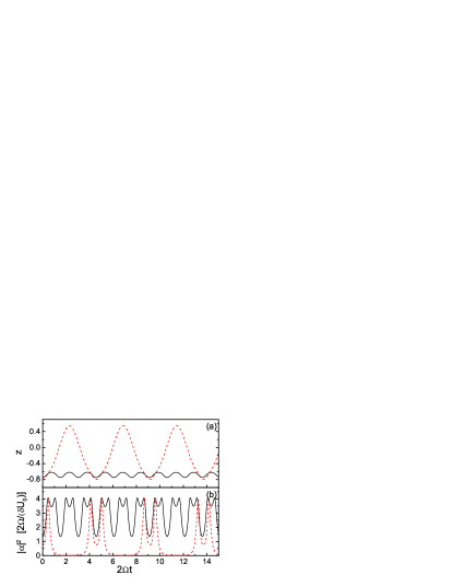
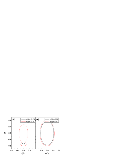
Figure 2: (Color online) Motion of the Bose Josephson junction. (a) Atom population imbalance $z$ and (b) intra-cavity photon number $|\alpha|^{2}$ [in units of $2\Omega/(\delta U_{0})$] versus the reduced time $2\Omega t$. The initial conditions are $(\phi(0),z(0))=(0,-0.75)$ (black solid lines) and $(\phi(0),z(0))=(0,-0.8)$ (red dashed lines). (c) and (d): trajectories of the Bose Josephson junction (c) coupled or (d) uncoupled to the cavity mode, with the two different initial conditions above. The same parameters as in Fig. 1.

We note that the cavity mode plays a dual role here. On one hand, it plays with the condensates interactively and modifies their dynamics effectively; on the other hand, it also carries with it the information of the population of the atoms between the two traps as it leaks out of the cavity. In Figs. 2(a)-(b), we plot the time evolution of the population imbalance and the number of intra-cavity photons (which is proportional to the cavity output), with the latter calculated from the former by using Eq. (8). Initially, the phase $\phi(0)=0$, and $z(0)=-0.75$, or $-0.8$, respectively. Despite of the minimal difference between the two initial states, the subsequent dynamics is quite different. The outputs of the cavity differ not only in their periods, but also in their detailed temporal structures. The trajectories of the BJJ, as can be read off from Fig. 1(b), are shown in Fig. 2(c). The influence of the cavity field on the BJJ dynamics can be seen by comparing Fig. 2(c) with Fig. 2(d). It is worth noting that this influence may occur at an extremely low intra-cavity photon number feasibility ; gupta . If the parameters can be determined independently, we may infer the population imbalance evolution from the outputs of the cavity. This may serve as a different approach, which is nondestructive, than the usual absorption image method, to track the tunneling dynamics of two weakly linked Bose-Einstein condensates. Of course, because the atom-field interaction involves only the atom numbers [see Eq. (4) or Eqs. (6) and (7)], no information of the relative phase of the two condensates is contained in the cavity outputs. To fully characterize the dynamics of a BJJ, techniques such as the release-and-interfere schumm ; albiez ; shin are still needed.

So far, we have assumed that the condensates remain intact during their interaction with the cavity mode. One concern is that, due to the temporal fluctuations of the intra-cavity photon number and hence the fluctuations of the intra-cavity optical lattice, some atoms may be diffracted into higher momentum modes meystre (this effect is sacrificed artificially here because of the two-mode approximation we adopt). However, thanks to the fact that the mean intra-cavity photon number here is very low (on the order of $0.01$, see feasibility ), the strength of the fluctuations of the optical lattice is small, so that this effect may be negligible. In fact, in Esslinger et al.’s experiment esslinger , where the mean intra-cavity photon number was maintained below $0.04$, which corresponded to a maximal lattice depth below $0.1$ recoil energy private , no signatures of diffraction were observed. Of course, the temporal fluctuations of the cavity field may heat the condensates and lead to atom loss, as has been observed experimentally colombe ; murch . In addition, it may also cause phase diffusion of the BJJ. These effects may damp the Josephson oscillation, and deserve further study.

In conclusion, we have derived an effective Hamiltonian for a Bose Josephson junction dispersively coupled to a single cavity mode, under the mean-field approximation. The change of the dynamics of the Bose Josephson junction is studied by the means of phase portraits. We gave just one example as in Fig. 1 for illustrative purposes. However, it by no means exhausts all the possibilities. In fact, by engineering the so many free parameters in the Hamiltonian, a large variety of qualitatively different cases are accessible. Although in this work, as a starting point, we have restricted to the time-independent case, it may be interesting to go into the time-dependent case. By using an external feedback depending on the outputs of the cavity rempe2 , in situ observation and manipulation of the state of a Bose Josephson junction may be achieved. Furthermore, generalization of the present scenario to a Josephson junction array, may be worth consideration. That will allow us to study the cavity-mediated long-range interactions rempe3 between far separated condensates.

This work was supported by NSF of China under Grant Nos. 90406017, 60525417, and 10775176, NKBRSF of China under Grant Nos. 2005CB724508, 2006CB921400, 2006CB921206, and 2006AA06Z104. J. M. Z. would like to thank S. Gupta and D. M. Stamper-Kurn for their kind help on understanding of their paper.

References

- (1) K. M. Fortier, S. Y. Kim, M. J. Gibbons, P. Ahmadi, and M. S. Chapman, Phys. Rev. Lett. 98, 233601 (2007).
- (2) A. D. Boozer, A. Boca, R. Miller, T. E. Northup, and H. J. Kimble, Phys. Rev. Lett. 97, 083602 (2006).
- (3) S. Nußmann, M. Hijlkema, B. Weber, F. Rohde, G. Rempe, and A. Kuhn, Phys. Rev. Lett. 95, 173602 (2005).
- (4) F. Brennecke, T. Donner, S. Ritter, T. Bourdel, M. Khl, and T. Esslinger, Nature 450, 268 (2007).
- (5) Y. Colombe, T. Steinmetz, G. Dubois, F. Linke, D. Hunger, and J. Reichel, Nature 450, 272 (2007).
- (6) R. H. Dicke, Phys. Rev. 93, 99 (1954).
- (7) J. M. Zhang, W. M. Liu, and D. L. Zhou, Phys. Rev. A 77, 033620 (2008).
- (8) S. Levy, E. Lahoud, I. Shomroni, and J. Steinhauer, Nature 449, 579 (2007).
- (9) S. Hofferberth, I. Lesanovsky, B. Fischer, J. Verdu, and J. Schmiedmayer, Nat. Phys. 2, 710 (2006).
- (10) T. Schumm, S. Hofferberth, L. M. Andersson, S. Wildermuth, S. Groth, I. Bar-Joseph, J. Schmiedmayer, and P. Krger, Nat. Phys. 1, 57 (2005).
- (11) M. Albiez, R. Gati, J. Folling, S. Hunsmann, M. Cristiani, and M. K. Oberthaler, Phys. Rev. Lett. 95, 010402 (2005).
- (12) Y. Shin, M. Saba, T. A. Pasquini, W. Ketterle, D. E. Pritchard, and A. E. Leanhardt, Phys. Rev. Lett. 92, 050405 (2004).
- (13) J. Klinner, M. Lindholdt, B. Nagorny, and A. Hemmerich, Phys. Rev. Lett. 96, 023002 (2006); Th. Elsser, B. Nagorny, and A. Hemmerich, Phys. Rev. A 69, 033403 (2004); B. Nagorny, Th. Elssser, and A. Hemmerich, Phys. Rev. Lett. 91, 153003 (2003).
- (14) S. Gupta, K. L. Moore, K. W. Murch, and D. M. Stamper-Kurn, Phys. Rev. Lett. 99, 213601 (2007).
- (15) G. J. Milburn, J. Corney, E. M. Wright, and D. F. Walls, Phys. Rev. A 55, 4318 (1997).
- (16) In contrast to the single atom case, here we have to take into account the collective behavior of the atoms. Thus the large detuning condition corresponds to , for all relevant pairs , see also the supplementary information of Ref. colombe .
- (17) I. B. Mekhov, C. Maschler, and H. Ritsch, Nat. Phys. 3, 319 (2007); C. Maschler and H. Ritsch, Phys. Rev. Lett. 95, 260401 (2005).
- (18) A. J. Leggett, Rev. Mod. Phys. 73, 307 (2001).
- (19) S. Raghavan, A. Smerzi, and V. M. Kenkre, Phys. Rev. A 60, R1787 (1999).
- (20) Its cavity mode coupled counterpart, may be referred to as a cavity mode “dressed” Bose Josephson junction, see also the concept of “dressed Bose-Einstein condensates” in E. V. Goldstein, E. M. Wright, and P. Meystre, Phys. Rev. A 57, 1223 (1998).
- (21) P. Horak, S. M. Barnett, and H. Ritsch, Phys. Rev. A 61, 033609 (2000).
- (22) A. Smerzi, S. Fantoni, S. Giovanazzi, and S. R. Shenoy, Phys. Rev. Lett. 79, 4950 (1997).
- (23) S. Raghavan, A. Smerzi, S. Fantoni, and S. R. Shenoy, Phys. Rev. A 59, 620 (1999).
- (24) S. Haroche, M. Brune, and J. M. Raimond, Europhys. Lett. 14, 19 (1991).
- (25) M. S. Chang, Q. Qin, W. Zhang, L. You, and M. S. Chapman, Nat. Phys. 1, 111 (2005).
- (26) V. I. Arnold, Ordinary Differential Equations, translated from the Russian by Richard A. Silverman (MIT Press, Cambridge, MA, 1973), p. 262.
- (27) P. Buonsante, R. Franzosi, and V. Penna, Phys. Rev. Lett. 90, 050404 (2003).
- (28) We think this set of parameters are experimentally practical. By taking Hz, Hz, Hz, , , , , we have , , . Note that is free by adjusting the cavity pump detuning.
- (29) Yu. B. Ovchinnikov, J. H. Mller, M. R. Doery, E. J. D. Vredenbregt, K. Helmerson, S. L. Rolston, and W. D. Phillips, Phys. Rev. Lett. 83, 284 (1999).
- (30) F. Brennecke (private communication).
- (31) K. W. Murch, K. L. Moore, S. Gupta, and D. M. Stamper-Kurn, Preprint at http://arxiv.org/abs/0706.1005 (2007).
- (32) P. W. H. Pinkse, T. Fischer, P. Maunz, and G. Rempe, Nature 404, 365 (2000); C. J. Hood, T. W. Lynn, A. C. Doherty, A. S. Parkins, and H. J. Kimble, Science 287, 1447 (2000).
- (33) P. Mnstermann, T. Fischer, P. Maunz, P.W. H. Pinkse, and G. Rempe, Phys. Rev. Lett. 84, 4068 (2000).