Gamma-Ray Bursts, new cosmological beacons

Abstract

Long Gamma-Ray Bursts (GRBs) are the brightest electromagnetic explosions in the Universe, associated to the death of massive stars. As such, GRBs are potential tracers of the evolution of the cosmic massive star formation, metallicity, and Initial Mass Function. GRBs also proved to be appealing cosmological distance indicators. This opens a unique opportunity to constrain the cosmic expansion history up to redshifts 5–6. A brief review on both subjects is presented here.

Los Estallidos de Rayos Gamma (ERG’s) largos son las explosiones electromagnéticas más potentes del Universo, asociadas a la muerte de estrellas masivas. Como tales, los ERG’s son trazadores potenciales de la evolución de la formación estelar cósmica, la metalicidad y la función inicial de masa. Los ERG’s también han probado ser atractivos como indicadores de distancia cosmológicos, lo cual abre una oportunidad única de constreñir la historia de expansión cósmica hasta $z\approx 5-6$. Se presenta aquí una reseña sobre ambos temas.

Cosmology: observations gamma–rays: bursts stars: star formation history

0.1 Introduction

Detected as brief ($\sim 0.01-100$ s), intense flashes of $\gamma$–rays (mostly sub–MeV), Gamma–ray Busts (GRBs) are the brightest electromagnetic explosions in the Universe. The power emitted by GRBs in electromagnetic form can reach luminosities up to $L\sim 10^{52}-10^{53}$ erg  s^-1, while AGNs can have $L\sim 10^{48}$ erg  s^-1  (but for long times), and Supernovae can have $L\sim 10^{45}$ erg  s^-1  for the first hundreds of seconds after the explosion. The short variability timescales of the $\gamma-$ray emission, suggest already very small dimensions for the sources, of the order of tens of kilometers, typical of stellar black holes or neutron stars. Several pieces of evidence indeed show that GRBs are associated with cataclysmic stellar events, and that the $\gamma-$ray emission comes from highly relativistic collimated outflows. The typical bulk Lorentz factor for the jets is $\Gamma\sim 300$. Thus, GRBs are true cosmic laboratories for the study of relativistic, magneto–hydrodynamical, and high energy processes (for recent reviews on the GRB physics see e.g., Zhang & Mészáros 2004; Piran 2005; Mészáros 2006).

Furthermore, GRBs and their afterglows are of great interest for studies related to stellar astrophysics, the interstellar and intergalactic medium, and most important, they reveal themselves as unique probes of the high redshift Universe. In the last 3 years, on average $\sim 1$ paper per day is published on GRBs in refereed journals and $\sim 4$ per day in non–refereed publications.

GRBs are divided into two main groups which, following the notation of Zhang (2007), we will call Type I and Type II. The former ($\approx 1/3$) have short $\gamma-$ray durations ($\lesssim 2$ s) and hard spectrum; it is conjectured that they result from binary mergers of compact stellar objects (NS–NS or NS–BH). The latter ($\approx 2/3$) have durations larger than 2 s and their $\gamma-$ray spectra tend to be softer. The observations show (e.g., Hjorth et al. 2003; Stanek et al. 2003) that these GRBs result from the collapse of rapidly rotating cores of low–metallicity stars more massive than about 25 M_⊙  (’collapsar’ scenario).

A breakthrough in the GRB field happened a decade ago: thanks to their relatively long duration, for some Type II GRBs it was possible to resolve and detect the afterglow at softer (X–ray, optical, IR and radio) energies. This allowed to measure spectral lines and/or to identify the host galaxy; hence the redshifts, $z$, could be determined. Up to December 2007, there were around 100 GRBs with secure $z$ measurements (in $\sim 90\%$ of the cases by the afterglow and $\sim 10\%$ of the cases by the host galaxy). More than 60% of the $z$ determinations were obtained during the last 3 years with the dedicated Swift  satellite (Gehrels et al. 2004), which allowed also to discover the afterglows for some Type I events (7 up to date). No doubt, GRBs are the brightest transient cosmological events measurable. In Fig. 1 the $z$ distribution of Swift  GRBs is shown: it ranges from $z=0.033$ to 6.29, with an average $z$ of 2.2. Indirect estimates suggest, however, that many of the observed Type II GRBs could be produced at $z^{\prime}$s larger than 6 (e.g., Bromm & Loeb 2005).

Summarizing: type II GRBs are extremely powerful explosions associated to the collapse of short–lived massive stars, with peak emission at sub–MeV energies, where dust extinction is not an issue. Besides, the $\gamma-$ray spectra of type II GRBs are such that the $K$ correction is small or even negative. Thus, the fluxes of these events can be detected eventually from any $z$. All these properties convert type II GRBs in cosmological beacons, which can help us look back in time. We will review here advances along this line in two directions: GRBs as tracers of the history of global massive star formation rate (SFR; §2), and GRBs as cosmic rulers able to help us in constraining the expansion history of the Universe (§3). In §4, perspectives for future work will be discussed.

0.2 GRBs as tracers of the global massive star formation rate

The death rate of massive short–lived stars resembles their formation rate. Thus, the GRB formation rate (GFR) can be used as a potential tracer of the massive SFR in the Universe. Current observations allow to construct the (yet very incomplete) GRB $z$ distribution per unit of time, $\dot{N}(z)$. This observable distribution is connected to the history of the intrinsic GFR (per unit of comoving volume), $\dot{n}_{\rm GRB}(z)$, through:

$$\mbox{$\dot{N}(z)$}=\int_{0}^{z}dz\frac{dV/dz}{1+z}\frac{F(z)}{f_{obs}}\mbox{$\dot{n}_{\rm GRB}(z)$},$$ (1)

where $dV/dz$ is the comoving volume element, $(1+z)^{-1}$ accounts for the time dilation, $f_{obs}$ stands for the detector exposure factor and the average GRB beaming, and $F(z)=\phi_{flux}(z)\phi_{z}(z)$ takes into account several selection effects. $F(z)$ can be understood as the probability to detect the burst and its afterglow, and to measure its $z$ from the afterglow; it comprises two classes of effects:

• the flux–limited selection function,

  $$\phi_{flux}(z)=\int_{\mbox{L${}_{\rm iso}$}(P_{\rm min},z)}^{\infty}\mbox{$f$(L${}_{\rm iso}$)dL${}_{\rm iso}$},$$ (2)

  which depends on the detector flux threshold $P_{\rm min}$ and on the GRB luminosity function (LF), $f$(L_iso)dL_iso  (L_iso  is the equivalent isotropic –beam uncorrected– GRB bolometric luminosity).

• the selection function related to the observability of the afterglow and its $z$ determination, $\phi_{z}(z)$. This function is very uncertain and comprises spectroscopic and photometric selection effects (e.g., observability of lines in the spectral range and in the presence of night–sky lines, afterglow flux–limited selection, different systematics in the emission or absorption line technique used to determine $z$), as well as potential astrophysical effects (e.g., obscuration, evolving dust extinction, a bias in the GRB host galaxy population). An evidence that these selection effects are severe is the fact that only $\sim 1/3$ of the Swift  GRBs have reliable $z$ determinations in spite of the quick afterglow localization and the great effort in follow–up observations.

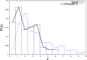
Figure 1: Normalized distribution of 72 spectroscopically measured $z^{\prime}$s obtained with Swift  (solid line) and 220 pseudo–redshifts obtained with the L_iso–variability correlation (dashed line).

0.2.1 Direct inferences, yet limited

A direct joint determination of $\dot{n}_{\rm GRB}(z)$  and $f$(L_iso)dL_iso  would be possible from a populated $\mbox{L${}_{\rm iso}$}-z$ diagram. However, the situation is complicated mainly by some of the uncertain component biases present in the $\phi_{z}(z)$ function (e.g., Bloom 2003; Gou et al. 2004; Fiore et al. 2007; Coward et al. 2007). In view of this and the yet low population statistics, it is not feasible to attempt a clean reconstruction of $\dot{n}_{\rm GRB}(z)$  from current data. Recent works that make use of the Swift  data start from some assumptions and limit themselves to explore only statistical compatibilities of the observed $\dot{N}(z)$  distribution with models of $\dot{n}_{\rm GRB}(z)$  assumed proportional to the global SFR history inferred from extragalactic studies, $\dot{\rho}_{\rm SFR}(z)$. A general conclusion is that $\dot{N}(z)$  implies an enhanced $\dot{n}_{\rm GRB}(z)$  at high redshifts with respect to $\dot{\rho}_{\rm SFR}(z)$  (Kistler et al. 2008; see also Le & Dermer 2007; Guetta & Piran 2007). It should be noted that some pieces of evidence suggest that the Swift  sample of GRBs with $z$ determined is a fair sample of the real high$-z$ GRB population (Fiore et al. 2007).

On the other hand, Coward et al. (2007) concluded that the observed Swift  $z-$distribution, where the number increasing from $z\approx 0$ to $z\approx 1.5$ is modest, implies a bias in the afterglow observability such that at $z=0-1$ it works inversely proportional to the global SFR history. It could be that the Swift  sample with $z$ is biased against low–$z$ GRBs, probably due to the enhanced extinction associated with the prolific SFR at $z\sim 1$ (Fiore et al. 2007; Coward et al. 2007).

0.2.2 Indirect inferences, encouraging results

Alternatively to the observed $\mbox{L${}_{\rm iso}$}-z$ diagram, there are other methods for inferring the GFR history from observations but in a model–dependent way. We will mention three methods:

(1) The most extensive GRB observational database is the CGRO-$BATSE$ peak flux $P$ distribution, $N(P)$, for $\sim 3000$ bursts. The $N(P)$  distribution (corrected by the exposure factor) is the result of 4 physical ingredients: $\dot{n}_{\rm GRB}(z)$, $f$(L_iso)dL_iso, the jet opening angle distribution, $f(\theta_{j}$), and the volumetric factor given by the cosmological model. Therefore, the inference of $\dot{n}_{\rm GRB}(z)$  from the observed $N(P)$  is a highly degenerated problem. The adequate introduction of complementary observational information helps to overcome partially the degeneracies; for example, the $E_{\rm pk}$  distribution (Daigne et al. 2006) or the $\theta_{j}$ distribution (Le & Dermer 2007).

(2) The $\mbox{L${}_{\rm iso}$}-z$ diagram can be (indirectly) obtained for large data-sets of GRBs without $z$ measured by using empirical correlations that involve L_iso. For example, Lloyd–Ronning et al. (2002) and Yonetoku et al. (2004) inferred $\dot{n}_{\rm GRB}(z)$  by applying the L_iso–variability correlation (Fenimore & Ramirez–Ruiz 2000) to 220 BATSE GRBs, and the $\mbox{L${}_{\rm iso}$}-E_{\rm pk,rest}$ relation to 689 BATSE GRBs, respectively. This method relies on the certainty and accuracy of the used empirical correlation.

(3) Given an adequate parametrization for $\dot{n}_{\rm GRB}(z)$  and $f$(L_iso)dL_iso, their free parameters can be efficiently constrained by fitting models jointly to both the observed $N(P)$  distribution and the $\dot{N}(z)$  distribution inferred as in (2) or as in §§2.1 after selection effects correction. So far, this method is the most powerful. A description of and the results from this method (Firmani et al. 2004; hereafter FAGT) are as follows.

The method. The observed $N(P)$  and $\dot{N}(z)$  distributions are modeled by seeding at each $z$ a large number of GRBs with a given rate, $\dot{n}_{\rm GRB}(z)$, and LF, $f$(L_iso)dL_iso, and then by propagating the flux of each source to $z=0$. L_iso in the rest frame is defined as L_iso=$\int_{\rm 30keV}^{\rm 10000keV}ES(E)dE$, where $S(E)$ is the Band (Band et al. 1993) energy spectrum. The break energy at rest, $E_{b}$, is assumed either constant (512 keV) or dependent on L_iso  according to the “Yonetoku relation” (Yonetoku et al. 2004). FAGT explored two models for $f$(L_iso)dL_iso, the single and double power laws (SPL and DPL, respectively), and two cases, one where $f$(L_iso)dL_iso  is constant in time, and another one where L_iso evolves as $(1+z)^{\delta}$. The function $\dot{n}_{\rm GRB}(z)$  was modeled as

$$\mbox{$\dot{n}_{\rm GRB}(z)$}=K\times e_{\rm SFR}(z;a,b)\times\eta_{z>2}(z;c),$$ (3)

where $e_{\rm SFR}(z;a,b)$ is a bi–parametric function proposed by Porciani & Madau (2000) for fitting the observed SFR history, and $\eta_{z>2}(z;c)$ allows to control the growth or decline of $\dot{n}_{\rm GRB}(z)$  at $z>2$. The idea is to constrain the parameters of the LF (2 and 3 for the SPL and DPL, and 1 more if evolution is allowed ) and of $\dot{n}_{\rm GRB}(z)$  (4 parameters) by applying a joint fit of the model predictions to the $N(P)$  and $\dot{N}(z)$  distributions. The $N(P)$  distribution for more than 3000 GRBs compiled by Stern et al. (2002) and the $z$ distribution inferred for 220 GRBs in Lloyd–Ronning et al. (2002; see above) were used.

Results. FAGT obtained that an evolving LF is preferred in all the analyzed cases (with an optimal value of $\delta=1\pm 0.2$). For non evolving LFs, the predicted $N(P)$  distributions have systematically an excess of GRBs at the bright end, and the peak of the $\dot{N}(z)$  distribution is shifted to higher $z^{\prime}$s (see their Fig. 1). Only a weak preference was found for the SPL model over the DPL one. On the other hand, the best fits not only imply an evolving LF but also GFRs histories that steeply increase (by a factor of $\sim 30$) from $z=0$ to $z\approx 2$ and then continue increasing gently up to $z\sim 10$ as $(1+z)^{1.4}$ and $(1+z)$ for the SPL and DPL LFs, respectively.

Figure 2 reproduces from FAGT the SFR history as traced by the GFR history (dot–shaded region) under an opportune normalization and assuming a constant initial mass function (IMF). Both the best SPL and DPL LF models with evolution ($\delta=1$) and their $1\sigma$ uncertainties are taken into account by the region. Symbols are the SFR traced by the rest–frame UV luminosity and corrected for dust obscuration (Giavalisco et al. 2004), while the solid line is a more recent piecewise fit to a large compilation and dust correction of SFR observations by Hopkins & Beacom (2006). The main difference between the SFR histories inferred from GRBs and from extragalactic observations is the enhancement (that increases with $z$) of the former with respect to the latter after $z=1-2$. Interesting enough, the Swift  based studies mentioned in §§2.1, while in much less detail, attain a similar conclusion.

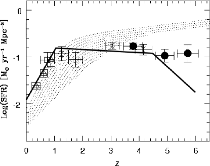
Figure 2: The cosmic SFR histories as traced by GRBs (dotted region) and by rest–UV luminosity (symbols and solid line, the latter from the recent fit to several observations by Hopkins & Beacom 2006); see text.

Implications. Why the GFR evolution might be enhanced with respect to the rest–UV traced SFR evolution at high redshifts? Let us discuss the pros and cons of some of the possibilities.

• Since the $\gamma-$rays do not suffer absorption, even in very dense molecular regions, GRBs are expected to trace the massive SFR of any galaxy/region in the Universe, for example of the dust–enshrouded actively star–forming galaxies at high redshifts. However, there are pieces of evidence against GRBs being located in this kind of galaxies (e.g., Le Floc’h et al. 2007).

• Most of the GRB host galaxies are faint, low–mass, low–metallicity star-forming galaxies (e.g., Fynbo et al. 2003; Stanek et al. 2006) and the GRB–to–SN ratio might increase significantly at lower metallicities (Yoon et al. 2006). Therefore, the GFR could be tracing the SFR of a biased population of low–metallicity galaxies. Nuza et al. (2007), by means of cosmological simulations, have found indeed that the GRB host properties are reproduced if GRBs form from low–metallicty progenitor stars. However, recent observational studies are showing that the neutral ISM around GRBs is not metal poor and is enriched by dust (see Savaglio 2007). Furthermore, GRB hosts should not to be special, but normal, faint, star-forming galaxies (the most abundant), detected at any $z$ just because a GRB event has occurred.

• If GRBs are produced in binary systems and the probability of interloper–catalyzed binary mergers in dense star clusters (where most GRBs appear to occur, Fruchter et al. 2006) increases with $z$, then an enhancement in the GFR is expected (Kistler et al. 2007). This scenario requires quantitative calculations. Interesting enough, FAGT, and more recently Bogomazov, Lipunov & Tutukov (2007), have calculated the Galaxy production rates of Wolf–Rayet stars in very close binaries (progenitors of rapidly rotating –Kerr– black holes), and found an approximate agreement with the estimated rates of type II GRBs in galaxies.

• An IMF that becomes increasingly top–heavy at higher $z$, would increase the relative number of massive stars produced. Since the rest–UV luminosity already traces massive SFR, the IMF should be biased to very massive stars (GRB progenitors) so that an evolving IMF could explain the difference seen in Fig. 2.

The above discussion is an example of the large potential of GRB studies for exploring such key issues in astronomy as SF at high $z$, and the IMF and chemical evolution in galaxies.

Regarding low $z^{\prime}$s, Fig. 2 shows that the GFR decays with time closely proportional to the SFR since $z\approx 1$. This feature does not seem to be observed in the Swift  $z$ distribution, which would imply a dominant redshfit bias, $\phi_{z}(z)$ as suggested by Coward et al. (2007). In the redshift range from $z=1$ to $z=2$, the SFR attains a broad maximum, while the GFR keeps increasing rapidly. The Swift  $z$ distribution would suggest the opposite. In fact, as shown in Fig. 1, the Swift  and the inferred from the $L-$variability relation $\dot{N}(z)$  distributions differ quite substantially up to $z\approx 2$ (rather than the absolute values, the important comparison between the two histograms is at the level of the fractional changes with $z$). As remarked by Fiore et al. (2007), the present samples with $z$ determinations seem to be largely incomplete, especially at $z\mathrel{\mathchoice{\lower 0.5pt\vbox{\par\halign{$\mathnew\displaystyle\hfil#\hfil$\cr<\crcr\sim\crcr}}}{\lower 0.5pt\vbox{\par\halign{$\mathnew\textstyle\hfil#\hfil$\cr<\crcr\sim\crcr}}}{\lower 0.5pt\vbox{\par\halign{$\mathnew\scriptstyle\hfil#\hfil$\cr<\crcr\sim\crcr}}}{\lower 0.5pt\vbox{\par\halign{$\mathnew\scriptscriptstyle\hfil#\hfil$\cr<\crcr\sim\crcr}}}}2$.

0.3 GRBs as tracers of the Universe expansion rate history

The energetics of GRBs spans 3–4 orders of magnitude; at first sight GRBs are all but standard candles. A breakthrough in the field happened after the discovery of a tight correlation between the collimation corrected bolometric energy, $E_{\gamma}=E_{\rm iso}(1-\cos\theta_{j})$ and the prompt peak energy in the $\nu f_{\nu}$ spectrum, $E_{\rm pk}$  (Ghirlanda et al. 2004a). This and any other similar correlations allow to standardize the GRB energetics for using GRBs as distance indicators in the Hubble diagram (HD). Such an endeavor, however, is not trivial.

The first conceptual problem is that most of the GRBs with $z$ measured are at cosmological distances (see Fig. 1). Therefore, the given correlation can not be calibrated locally; to establish the correlation, a cosmology should be assumed, but the cosmological parameters are just what we pretend to constrain in the HD. By using statistical approaches, this circularity problem can be treated in order to get optimal constraints for the explored cosmological parameters. The idea is to use the best–fitted correlation (smallest scatter) for each cosmology and to find which cosmology produces the smallest $\chi^{2}$ in the HD, constructed by applying the corresponding correlation. A powerful Bayessian–like method to carry out this undertaking has been introduced by Firmani et al. (2005,2007). Other groups have developed alternative variants (see e.g., Xu, Dai & Liang 2005; Schaefer 2007; Li et al. 2007). On the other hand, Ghirlanda et al. (2006) have shown that in order to calibrate for example the “Ghirlanda” correlation it is enough to have a dozen of GRBs in a narrow ($\Delta z/z\sim 0.1$) redshift bin, something that will be possible in the near future.

Results. The first cosmological results obtained by using the “Ghirlanda” correlation were encouraging: they provided a test of the accelerated expansion independent from the SN Ia studies (Ghirlanda et al. 2004b; Firmani et al. 2005; see also Dai, Liang & Xu 2004). The addition of GRBs to the SN probe, reduces the confidence levels of the constrained cosmological parameters. A drawback of the “Ghirlanda” correlation is that it needs to establish expensive follow–up observations: $\theta_{j}$ is determined from the achromatic break time, $t_{\rm break}$, in the afterglow light curve.

Firmani et al. (2006a) discovered a tight correlation among three prompt emission GRB parameters: L_iso, $E_{\rm pk}$, and duration t₄₅. Some of the cosmological constraints obtained by using the “Firmani” correlation are plotted in Fig. 3. We show in these plots how the confidence levels given by the SNLS survey (Astier et al. 2006) are improved when the GRB constraints are added. Right panel of Fig. 3 shows the HD for 117 SNLS supernovae and 19 GRBs by using the ’vanilla’ $\Lambda$CDM cosmology (solid line), which provides a good fit to the observations. GRBs are a natural extension of SNIa to high $z^{\prime}$. In the bottom panel the residuals to the assumed cosmology are plotted; the averages and its uncertainties are $0.15\pm 0.01$ mag and $0.26\pm 0.05$ mag for the SNe and GRBs, respectively.

Our results in general (constraining only two parameters at the same time) showed that the flat $\Lambda$CDM cosmology is consistent at the $1\sigma$ level with the HD of GRBs (and GRBs+SNe) up to $z=4.5$.

The cosmography with GRBs opens a valuable window for exploring the expansion history of the Universe to $z>2$ (more than $\sim$10 Gyr ago), where SNIa are practically impossible to observe. Besides, GRBs offer some important advantages for cosmographic studies. (1) GRBs are not affected by dust extinction. (2) The luminous distance $d_{L}$ in the HD is a cumulative quantity with $z$, so that the differences among different cosmological models become larger at higher $z^{\prime}$s. Thus, data-points in the HD at high $z^{\prime}$s highly discriminate the models, even if the uncertainties are large. (3) Each point in the HD translates into a different curve in the space of the cosmological parameters (degeneration). The wider in $z$ is the data sample, the less elongated along one curve (less degeneration) will be the parameter confidence levels (Firmani et al. 2007).

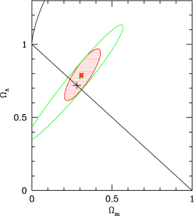
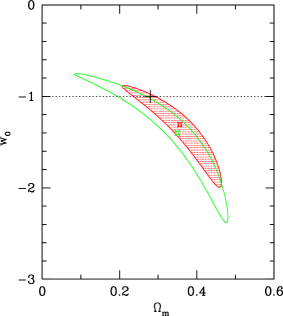
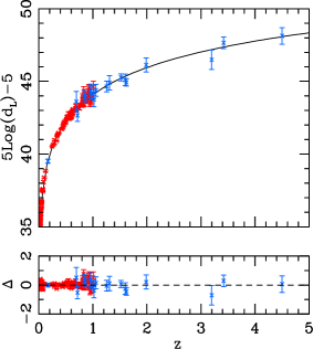
Figure 3: Left: Contours at 68.3% CL’s on the ($\Omega_{\rm m}$,$\Omega_{\Lambda}$) plane from the SNIa HD using our Bayesian approach to circumvent the circularity problem (solid green line) and from the combined SNIa+GRB HD (red shaded region). Middle: Same as left panel but on the ($\Omega_{\rm m}$, $w_{0}$) plane assuming flatness; $w_{0}$  is the equation of state index, assumed to be constant. Rigth: 117 SNIa (red) and 19 GRB (blue) data-points in the HD for the flat $\Lambda$CDM model. The residuals of the data-points minus the $\Lambda$CDM model are shown in the bottom panel.

Caveats. GRB cosmography is in its infancy and of course there should be several caveats as was discussed in the literature (e.g., Friedman & Bloom 2005). For example, it was argued that when using the “Ghirlanda” relation, the results are strongly dependent on the assumption about the density distribution of the circumbust medium (the dependence of $\theta_{j}$ on $t_{\rm break}$ changes slightly with the distribution assumed, and the parameters of one or another distribution are included in the calculation of $\theta_{j}$). Despite that the “Ghirlanda” correlations are different in one case or another, from the point of view of cosmography, the results are very similar (Nava et al. 2006). Furthermore, it was shown that an empirical correlation among E_iso, $E_{\rm pk}$, and $t_{\rm break}$ holds (avoiding then the assumption of the circumbust density distribution), which gives cosmographic results similar to those obtained with the “Ghirlanda” correlations (Liang & Zhang 2006). Recent Swift  observations have shown that the $X-$ray afterglow light curve is more complex than previously though and its break time tends to be different from the one inferred in the optical bands. Several pieces of evidence suggest that the $X-$ray and optical components come from different emitting regions; therefore, the requirement that the optical $t_{\rm break}$ should be compatible with the $X-$ray one should be relaxed (Nava et al. 2007).

Concerning the “Firmani” correlation, it was established for prompt $\gamma-$ray emission quantities alone. Therefore, it is model independent and does not requires follow–up observations. Some of the potential difficulties mentioned in general for the methods of standardizing the energetics of GRBs are the systematics and outliers in the correlations, the gravitational lensing, the possible evolution of GRB properties, and the lack of a physical interpretation of the correlations. We refer the reader to Ghisellini (2007), Firmani et al. (2007), and Ghirlanda (2007) for discussions on these caveats. In our opinion, the last problem is the most challenging. The possibility of evolution is also real (FAGT; Li 2007), but is most likely that this happens at the level of the overall population and not in what concerns the internal emission mechanisms, which control the spectral energy relations.

Finally, it should be said that the current samples of usable GRBs for the correlations involving energetics are still small. As the samples will increase in number, a better treatment of systematics and selection effects will be possible. On the other hand, a wide spectral $\gamma-$ray coverage is necessary in order to obtain reliable correlations involving the energetics of GRBs. Unfortunately, the Swift  BAT detector has a too narrow spectral coverage.

In our view, the use of GRBs as cosmological distance indicators has not been sufficiently appreciated by the astronomical community. We are aware of the difficulties of the method, but it should be considered that GRBs offer a unique possibility to constrain the expansion history of the Universe at $z>2$, and in a way that simply extends (and complements) the method based on SNe type Ia. Perhaps we are now in a similar situation as the SN Ia workers in the early 90’s, when the astronomical community used to react skeptically to their proposals. However, the effort is worth it, because the cosmography with GRBs may offer valuable information to unveil the properties of what we call Dark Energy, the big mystery of cosmology. This mystery stimulates now the frontiers of physics to move in the direction of exploring new elements of high energy physics, the unification of gravity and quantum physics, gravity beyond Einstein relativity, and extra dimensions.

0.4 Outlook

The inference of GFR history and its comparison with the cosmic SFR history will highly benefit from the growth of the samples of GRBs with accurate $z$ determination. However, as discussed in §§2.1, the selection effects that plague these samples are a challenging issue. Therefore, the indirect methods for inferring the GFR history (§§2.3) should be improved in parallel. These methods would largely benefit if large samples of GRBs with pseudo–redshifts are constructed. The use of correlations among prompt $\gamma-$ray quantities alone (e.g., the “Firmani” correlation) is the best way for this aim.

The improvement of the known GRB tight correlations or the discovery of new ones, is not only important for GFR studies but also for cosmography at high $z^{\prime}$s as shown in §3. The increasing of the observational data is mandatory in this endeavor. With a sample of $\sim 150$ GRBs, on one hand, the empirical correlations might already be calibrated in a small $z$ bin, and in the other one, the HD would become highly populated as to get tight constraints on the cosmological parameters. However, it should be noted that for the correlations that involve energetics and spectral information, a wide spectral coverage is necessary, something in which the Swift  detector fails. The hope is in feature missions as GLAST.