A Localization Approach to Improve Iterative Proportional Scaling in Gaussian Graphical Models

Abstract

We discuss an efficient implementation of the iterative proportional scaling procedure in the multivariate Gaussian graphical models. We show that the computational cost can be reduced by localization of the update procedure in each iterative step by using the structure of a decomposable model obtained by triangulation of the graph associated with the model. Some numerical experiments demonstrate the competitive performance of the proposed algorithm.

1 Introduction

Since Dempster Dempster introduced a multivariate Gaussian graphical model, also called a covariance selection model, it has been investigated by many authors from both theoretical and practical viewpoints. On the theory of a Gaussian graphical model, see e.g. Whittaker Whittaker , Lauritzen lauritzen1996 , Cox and Wermuth Cox-Wermuth and Edwards Edwards . In recent years much effort has been devoted to application of the Gaussian graphical model to identify sparse large network systems, especially genetic networks (e.g. Dobra , Li-Gui , Drton-2 ), and the efficient implementation of the inference in the model has been extensively studied. In this article we discuss an efficient algorithm to compute the maximum likelihood estimator (MLE) of the covariance matrix in the Gaussian graphical models.

When the graph associated with the model is a chordal graph, the model is called a decomposable model. For a decomposable model, the MLE of the covariance matrix is explicitly obtained. For general graphical models other than decomposable models, however, we need some iterative procedure to obtain the MLE. The iterative proportional scaling (IPS) procedure is one of popular algorithms to compute the MLE.

The IPS was first introduced by Deming and Stephan Deming-Stephan to estimate cell probabilities in contingency tables subject to certain fixed marginals. Its convergence and statistical properties have been well studied by many authors (e.g. Ireland-Kullback , Fienberg ) and the IPS have been justified in a more general framework (Csiszar ). Speed and Kiiveri Speed-Kiiveri first formulated the IPS in a Gaussian graphical model and gave a proof of its convergence.

However, from a practically point of view, a straightforward application of the IPS is often computationally too expensive for larger models. In the contingency tables several techniques have been developed to reduce both storage and computational time of the IPS (e.g. Jirousek , Jirousek-Preucil ). Badsberg and Malvestuto Badsberg-Malvestuto proposed a localized implementation of the IPS by using the structure of decomposable models containing the graphical model. Such a technique is called the chordal extension. The local computation based on the chordal extension has been a popular technique in many fields for numerical computation of a sparse linear system(e.g. Rose , FKMN ).

In the present paper we describe a localized algorithm based on the chordal extension for improving the computational efficiency of the IPS in the Gaussian graphical models. Let $\Delta$ be the set of variables which corresponds to the set of vertices of the graph associated with the model. The straightforward implementation of the IPS requires approximately $O(|\Delta|^{3})$ time in each iterative step for large models. In the similar way to the technique in Badsberg and Malvestuto Badsberg-Malvestuto , we localize the update procedure in each step by using the structure of a decomposable model containing the model. The proposed algorithm is shown to require $O(|\Delta|)$ time for some models.

The problem of computing the MLE is equivalent to the positive definite matrix completion problem. The proposed algorithm based on the chordal extension is closely related to the technique discussed by Fukuda et al. FKMN in the framework of the positive definite matrix completion problem but not the same.

As pointed out in Dahl et al. Dahl , the implementation of the IPS requires enumeration of all maximal cliques of the graph and this enumeration has an exponential complexity. Hence the application of the IPS to large models may be limited. However in the case where the model is relatively small or the structure of the model is simple, it may be feasible to enumerate maximal cliques. In this article we consider such situations.

The organization of this paper is as follows. In Section 2 we summarize notations and basic facts on graphs and give a brief review of Gaussian graphical models and the IPS algorithm for covariance matrices. In Section 3 we propose an efficient implementation of the update procedure of the IPS. In Section 4 we perform some numerical experiments to illustrate the effectiveness of the proposed procedure. We end this paper with some concluding remarks in Section 5.

2 Background and preliminaries

2.1 Preliminaries on decompositions of graphs

In this section we summarize some preliminary facts on decompositions of graphs needed in the argument of the following sections according to Leimer Leimer , Lauritzen lauritzen1996 and Malvestuto and Moscarini Malvestuto-Moscarini .

Let ${\cal G}=(\Delta,E)$ be an undirected graph, where $\Delta$ denotes the set of vertices and $E$ denotes the set of edges. A subset of $\Delta$ which induces a complete subgraph is called a clique of ${\cal G}$. Define the set of maximal cliques of ${\cal G}$ by ${\cal C}$. For a subset of vertices $V$, let ${\cal G}(V)$ denote the subgraph of ${\cal G}$ induced by $V$. When a graph ${\cal G}$ is not connected, we can consider each connected component of ${\cal G}$ separately. Therefore we only consider a connected graph from now on.

A subset $S\subset\Delta$ is said to be a separator of ${\cal G}$ if ${\cal G}(\Delta\setminus S)$ is disconnected. For a separator $S$, a triple $(A,B,S)$ of disjoint subsets of $\Delta$ such that $A\cup B\cup S=\Delta$ is said to form a decomposition of ${\cal G}$. A separator $S$ is called a clique separator if $S$ is a clique of ${\cal G}$. For two non-adjacent vertices $\delta$ and $\delta^{\prime}$, $S\subset\Delta$ is said to be a $(\delta,\delta^{\prime})$-separator if $\delta\in A$ and $\delta^{\prime}\in B$ for a decomposition $(A,B,S)$. A $(\delta,\delta^{\prime})$-separator which is minimal with respect to inclusion relation is called a minimal $(\delta,\delta^{\prime})$-separator or a minimal vertex separator(Lauritzenlauritzen1996 ). Denote by ${\cal S}$ the set of minimal vertex separators for all non-adjacent pairs of vertices in ${\cal G}$.

A graph ${\cal G}$ is called reducible if $\Delta$ contains a clique separator and otherwise ${\cal G}$ is said to be prime. If ${\cal G}(V)$ is prime and ${\cal G}(V^{\prime})$ is reducible for all $V^{\prime}$ with $V\subsetneq V^{\prime}\subset\Delta$, ${\cal G}(V)$ is called a maximal prime subgraph (mp-subgraph) of ${\cal G}$. For any reducible graph, its decomposition into mp-subgraphs is uniquely defined(LeimerLeimer , Malvestuto and MoscariniMalvestuto-Moscarini ). Denote by ${\cal V}$ the set of subsets of $\Delta$ which induces mp-subgraphs of ${\cal G}$ and let $|{\cal V}|=M$. Then there exists a sequence $V_{1},\dots,V_{M}\in{\cal V}$ such that for every $m=2,\ldots,M$ there exists $m^{\prime}<m$ with

$$V_{m^{\prime}}\supset V_{m}\cap(V_{1}\cup\cdots\cup V_{m-1}).$$

Such a sequence is called a D-ordered sequence. Let $S_{m}:=V_{m}\cap(V_{1}\cup\cdots\cup V_{m-1})$ for $m=2,\ldots,M$. Define $\bar{\cal S}=\{S_{2},\dots,S_{m}\}$. Denote by ${\cal S}_{C}$ the set of clique separators of ${\cal G}$. Then $\bar{\cal S}$ satisfy $\bar{\cal S}={\cal S}\cap{\cal S}_{C}$. So we call elements of $\bar{\cal S}$ clique minimal vertex separators. LeimerLeimer showed that reducible graphs always have a D-ordered sequence with $V_{1}=V$ for any $V\in{\cal V}$. Hence a D-ordered sequence is not uniquely defined. However $\bar{\cal S}$ is common for all D-ordered sequences.

Example 1 (A reducible graph).

The graph ${\cal G}$ in Figure 1 is an example of reducible graphs. ${\cal G}$ has two clique minimal vertex separators $S_{2}:=\{3,4\}$ and $S_{3}:=\{5,6\}$. Define $V_{1}$, $V_{2}$ and $V_{3}$ by

$$V_{1}:=\{1,2,3,4\},\quad V_{2}:=\{3,4,5,6\},\quad V_{3}:=\{5,6,7,8\}$$

as in Figure 1. Then ${\cal V}=\{V_{1},V_{2},V_{3}\}$ and the sequence $V_{1}$, $V_{2}$, $V_{3}$ is a D-ordered sequence.

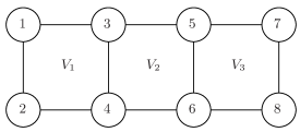
Figure 1: A reducible graph with eight vertices

When ${\cal G}$ is a chordal graph, ${\cal V}$ and $\bar{\cal S}$ are equal to the set of maximal cliques ${\cal C}$ and the set of minimal vertex separators ${\cal S}$ of ${\cal G}$, respectively. Hence $|{\cal C}|=M$. A D-ordered sequence for a chordal graph is called a perfect sequence of maximal cliques. There exists a perfect sequence of maximal cliques $C_{1},\ldots,C_{M}$ such that $C_{1}=C$ for any $C\in{\cal C}$(e.g. Lauritzenlauritzen1996 ).

For a vertex $\delta\in\Delta$, let $\mathrm{adj}(\delta)$ denote the set of vertices adjacent to $\delta$. When $\mathrm{adj}(\delta)$ is a clique, $\delta$ is called a simplicial vertex. A simplicial vertex is contained in only one maximal clique $C$. Hence if $\delta$ is simplicial and $\delta\in C$, then $\mathrm{adj}(\delta)=C\setminus\{\delta\}$. A sequence of vertices $\delta_{1},\delta_{2},\ldots,\delta_{|\Delta|}$ is called a perfect elimination order of vertices of ${\cal G}$ if $\delta_{i}$ is a simplicial vertex in ${\cal G}(\bigcup_{j=i}^{|\Delta|}\{\delta_{j}\})$. It is well known that ${\cal G}$ is a chordal graph if and only if ${\cal G}$ possesses a perfect elimination order (DiracDirac ). Let $C_{1},\ldots,C_{M}$ be a perfect sequence of maximal cliques of a chordal graph ${\cal G}$. Define $R_{1}:=C_{1}\setminus S_{2}$, $S_{m}:=C_{m}\cap(C_{1}\cup\cdots\cup C_{m-1})$ and $R_{m}:=C_{m}\setminus S_{m}$ for $m=2,\ldots,M$. Let $r_{m}:=|R_{m}|$. Let $\delta^{m}_{1},\ldots,\delta^{m}_{r_{m}}$ be any sequence of vertices in $R_{m}$. Then the sequence of vertices

$$\delta^{M}_{1},\ldots,\delta^{M}_{r_{M}},\delta^{M-1}_{1},\ldots,\delta^{M-1}_{r_{M-1}},\ldots,\delta^{1}_{1},\ldots,\delta^{1}_{r_{1}}$$

is a perfect elimination order of ${\cal G}$. We call it a perfect elimination order induced by the perfect sequence $C_{1},\ldots,C_{M}$.

We introduce some notations and a basic formula for matrices needed in the following sections. Let $A=\{a_{ij}\}$ be a $|\Delta|\times|\Delta|$ matrix. For two subsets $\Delta_{1}$ and $\Delta_{2}$ of $\Delta$, we let

$$A_{\Delta_{1}\Delta_{2}}=\{a_{ij}\}_{i\in\Delta_{1},j\in\Delta_{2}}$$

denote a $|\Delta_{1}|\times|\Delta_{2}|$ submatrix of $A$. Define

$$A_{\Delta_{1}\Delta_{2}}^{-1}:=(A^{-1})_{\Delta_{1}\Delta_{2}}.$$

We let $[A_{\Delta_{1}\Delta_{2}}]^{\Delta}$ denote the $|\Delta|\times|\Delta|$ matrix such that

$$([A_{\Delta_{1}\Delta_{2}}]^{\Delta})_{ij}=\left\{\begin{array}[]{ll}a_{ij}&\text{ if }i\in\Delta_{1},j\in\Delta_{2}\\ 0&\text{ otherwise }.\end{array}\right.$$

Let $\Delta_{2}=\Delta_{1}^{C}$ and decompose a symmetric matrix $A$ into blocks as

$$A=\left(\begin{array}[]{cc}A_{\Delta_{1}\Delta_{1}}&A_{\Delta_{1}\Delta_{2}}\\ A^{\prime}_{\Delta_{1}\Delta_{2}}&A_{\Delta_{2}\Delta_{2}}\\ \end{array}\right).$$

Here for notational simplicity we displayed $A$ for the case that the elements of $\Delta_{1}$ are smaller than those of $\Delta_{2}$. Suppose that $A_{\Delta_{2}\Delta_{2}}$ and $A_{\Delta_{1}\Delta_{1}}-A_{\Delta_{1}\Delta_{2}}(A_{\Delta_{2}\Delta_{2}})^{-1}A^{\prime}_{\Delta_{1}\Delta_{2}}$ are both positive definite. Then $A$ is positive definite and

$$A^{-1}_{\Delta_{1}\Delta_{1}}=\left(A_{\Delta_{1}\Delta_{1}}-A_{\Delta_{1}\Delta_{2}}(A_{\Delta_{2}\Delta_{2}})^{-1}A^{\prime}_{\Delta_{1}\Delta_{2}}\right)^{-1}.$$ (1)

2.2 Gaussian graphical models

Let ${\cal M}^{+}({\cal G})$ denote the set of $|\Delta|\times|\Delta|$ positive definite matrices $K=\{k_{ij}\}$ such that $k_{ij}=0$ for all $i$, $j\in\Delta$ with $i\neq j$ and $(i,j)\notin E$. Then the Gaussian graphical model for $|\Delta|$ dimensional random variable $Y=(Y^{(1)},\ldots,Y^{(|\Delta|)})^{\prime}$ associated with a graph $\cal G$ is defined as

$$Y\sim N_{|\Delta|}(\mu,\Sigma),\quad K:=\Sigma^{-1}\in{\cal M}^{+}({\cal G}).$$

$k_{ij}=0$ indicates the conditional independence between $Y^{(i)}$ and $Y^{(j)}$ given all other variables. In what follows, we identify ${\cal M}^{+}({\cal G})$ with the corresponding graphical model. Let $y_{1},\ldots,y_{n}$ be i.i.d. samples from ${\cal M}^{+}({\cal G})$. Define $\bar{y}$ and $W$ by

$$\bar{y}:=n^{-1}\sum_{i=1}^{n}y_{i},\quad W:=\sum_{i=1}^{n}(y_{i}-\bar{y})(y_{i}-\bar{y})^{\prime},$$

respectively. The likelihood equation is written as

$$L(\mu,K)\propto(\mathrm{det}K)^{n/2}\exp\left\{-\frac{1}{2}\mathrm{tr}KW-\frac{n}{2}\mathrm{tr}K(\bar{y}-\mu)(\bar{y}-\mu)^{\prime}\right\}.$$

The MLE of $\mu$ is $\bar{y}$. The likelihood equations involving $K$ are expressed as

$$nK^{-1}_{CC}=n\Sigma_{CC}=W_{CC},\quad\forall C\in{\cal C}.$$ (2)

For a subset of vertices $V\subset\Delta$, let $\hat{K}_{VV}$ denote the MLE of $K$ in the marginal model associated with the graph ${\cal G}(V)$ based on the data in $V$-marginal sample only. Let $S$ be a clique separator of ${\cal G}$ and $(A,B,S)$ be a decomposition of ${\cal G}$. Let $V=A\cup S$ and $V^{\prime}=B\cup S$. Then the MLE $\hat{K}$ is known to satisfy

$$\hat{K}=\left[\hat{K}_{VV}\right]^{\Delta}+\left[\hat{K}_{V^{\prime}V^{\prime}}\right]^{\Delta}-n\left[(W_{SS})^{-1}\right]^{\Delta}$$ (3)

(e.g. Lauritzen lauritzen1996 ). More generally, for the set of mp-subgraphs ${\cal V}$ and the set of clique minimal vertex separators $\bar{\cal S}$,

$$\hat{K}=\sum_{V\in{\cal V}}\left[\hat{K}_{VV}\right]^{\Delta}-n\sum_{S\in\bar{\cal S}}\left[(W_{SS})^{-1}\right]^{\Delta}.$$ (4)

As mentioned in the previous section, when the model is decomposable, ${\cal V}={\cal C}$ and ${\cal S}=\bar{\cal S}$. Hence from (2), $\hat{K}$ is explicitly written by

$$\hat{K}=n\sum_{C\in{\cal C}}\left[(W_{CC})^{-1}\right]^{\Delta}-n\sum_{S\in{\cal S}}\left[(W_{SS})^{-1}\right]^{\Delta}.$$

However for other graphical models, we need some iterative procedure for computing the first term on the right-hand side of (4). The following IPS is commonly used for this purpose. Note that the second term on the right-hand side of (4) needs to be calculated only once and is not involved in the iterative procedure. IPS consists of iteratively and successively adjusting $\Sigma_{CC}$ for $C\in{\cal C}$ as in (2). Let $K^{t}$ and $\Sigma^{t}=(K^{t})^{-1}$ denote the estimated $K$ and $\Sigma$ at the $t$-th step of iteration, respectively. Define $D:=\Delta\setminus C$ for $C\in{\cal C}$. Then the $t$-th iterative step of the IPS is described by the update rule of $K^{t}$ as follows.
Algorithm 0 (Iterative proportional scaling for $K$)

Step 0

$t\leftarrow 1$ and select an initial estimate $K^{0}$ such that $K^{0}\in{\cal M}^{+}({\cal G})$.

Step 1

Select a maximal clique $C\in{\cal C}$ and update $K$ as follows,

$$(K^{t})_{CC} \leftarrow(W_{CC})^{-1}+(K^{t-1})_{CD}((K^{t-1})_{DD})^{-1}(K^{t-1})_{DC}$$ (5)

$$(K^{t})_{CD} \leftarrow(K^{t-1})_{CD}$$

$$(K^{t})_{DD} \leftarrow(K^{t-1})_{DD}.$$

Step 2

If $K^{t}$ converges, exit. Otherwise $t\leftarrow t+1$ and go to Step 1.

From (1), it is easy to see that

$$(K^{t})^{-1}_{CC}=(\Sigma^{t})_{CC}=W_{CC}/n.$$

In Step 1, only the $C$-marginal of $K$ is updated. Therefore we note that if the initial estimate $K^{0}$ satisfies $K^{0}\in{\cal M}^{+}({\cal G})$, $K^{t}$ satisfies $K^{t}\in{\cal M}^{+}({\cal G})$ for all $t$. By using the argument of Csiszár Csiszar , the convergence of the algorithm to the MLE

$$\lim_{n\to\infty}K^{t}=\hat{K},\quad\lim_{n\to\infty}\Sigma^{t}=\hat{\Sigma}$$

is guaranteed (Speed and Kiiveri Speed-Kiiveri and Lauritzen lauritzen1996 ).

The fact (3) suggests that the decomposition $(A,B,S)$ for a clique separator $S$ can localize the problem, that is, in order to obtain the MLE $\hat{K}$, it suffices to compute the MLE of submatrix $\hat{K}_{VV}$ and $\hat{K}_{V^{\prime}V^{\prime}}$, where $V=A\cup S$ and $V^{\prime}=B\cup S$. Especially if the decomposition by mp-subgraphs is obtained, we need only to compute $\hat{K}_{VV}$ for each $V\in{\cal V}$.

From a complexity theoretic point of view, the $t$-th iterative step (5) requires $O(|D|^{3}+|D|^{2}|C|+|D||C|^{2})$ time. The graphical model with

$${\cal C}=\{\{1,2\},\{2,3\},\ldots,\{|\Delta|-1,|\Delta|\},\{|\Delta|,1\}\}$$

is called the $|\Delta|$-dimensional cycle model or $|\Delta|$ cycle model. Note that the cycle is prime. In the case of $|\Delta|$ cycle model, $|C|=2$ and $|D|=|\Delta|-2$. Hence when $|\Delta|\geq 4$, the iterative step (5) requires $O((|\Delta|-2)^{3})$ time. In the next section we propose a more efficient algorithm for computing (5) by using the structure of a chordal extension of a graph.

3 A localized algorithm of IPS

From (1), we note that (5) is rewritten as

$$(K^{t})_{CC} =(W_{CC})^{-1}+(K^{t-1})_{CC}-((\Sigma^{t-1})_{CC})^{-1}$$

$$=(W_{CC})^{-1}+(K^{t-1})_{CC}-((K^{t-1})^{-1}_{CC})^{-1}.$$ (6)

In this section we provide an efficient algorithm to compute $((K^{t-1})^{-1}_{CC})^{-1}$ by using the structure of ${\cal G}$. For a graph ${\cal G}$, let ${\cal G}^{*}$ be a chordal graph obtained by triangulating ${\cal G}$. Such ${\cal G}^{*}$ is called a chordal extension of ${\cal G}$. Figure 2 represents an example of the five cycle model and its chordal extension.

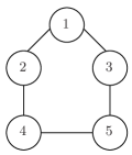
(i) the five cycle model	(ii) a chordal extension of (i)

Figure 2: The five cycle model and its chordal extension

Let $C^{*}_{1},\ldots,C^{*}_{M}$ be a perfect sequence of the maximal cliques of ${\cal G}^{*}$ with $C^{*}_{1}\supset C$. Let $S^{*}_{m}:=C^{*}_{m}\cap(C^{*}_{1}\cup\cdots\cup C^{*}_{m-1})$ for $m=2,\ldots,M$ be minimal vertex separators of ${\cal G}^{*}$. We propose the following algorithm to compute $((K^{t-1})^{-1}_{CC})^{-1}$ for each maximal clique $C\in{\cal C}$.

Algorithm 1 (Computing $((K^{t-1})^{-1}_{CC})^{-1}$).

Step 0

$m\leftarrow M$ and $K^{*}\leftarrow K^{t-1}$.

Step 1

If $m\neq 1$, select a simplicial vertex $\delta\in C_{m}^{*}$ of ${\cal G}^{*}$.
    If $m=1$, select a vertex $\delta\notin C$.
    Let $Q=C_{m}^{*}\setminus\{\delta\}$.

Step 2

Update $K^{*}_{QQ}$ by

$$K^{*}_{QQ}\leftarrow K^{*}_{QQ}-(k^{*}_{\delta\delta})^{-1}K^{*}_{Q\delta}K^{*}_{\delta Q}.$$ (7)

Step 3

Update $C^{*}_{m}$, ${\cal G}^{*}$ and $\Delta$ as follows,

$$C^{*}_{m}\leftarrow Q,\quad{\cal G}^{*}\leftarrow{\cal G}^{*}(\Delta\setminus\{\delta\}),\quad\Delta\leftarrow\Delta\setminus\{\delta\}.$$

If $C^{*}_{m}=S^{*}_{m}$, $m\leftarrow m-1$.
    If $C^{*}_{m}=C$, return $K^{*}_{CC}$. Otherwise, go to Step 1.

Now we state the main theorem of this paper.

Theorem 1.

The output $K^{*}_{CC}$ of Algorithm 1 is equal to $((K^{t-1})^{-1}_{CC})^{-1}$.

Proof.

Let $\delta\in C^{*}_{M}$ be a simplicial vertex in ${\cal G}^{*}$. Define $Q:=C^{*}_{M}\setminus\{\delta\}$, $Q_{1}:=\Delta\setminus\{\delta\}$ and $Q_{2}:=\Delta\setminus C^{*}_{M}$. Since $\mathrm{adj}(\delta)\subset C^{*}_{M}$ and $K^{(t-1)}\in{\cal M}^{+}({\cal G})$, $(K^{t-1})_{Q_{2}\delta}=\bm{0}$. Noting that $Q\cup Q_{2}=Q_{1}$, we have from (1)

$$((K^{t-1})_{Q_{1}Q_{1}}^{-1})^{-1} =(K^{t-1})_{Q_{1}Q_{1}}-(k^{t-1})^{-1}_{\delta\delta}(K^{t-1})_{Q_{1}\delta}(K^{t-1})_{\delta Q_{1}}$$

$$=(K^{t-1})_{Q_{1}Q_{1}}-(k^{t-1})^{-1}_{\delta\delta}\left(\begin{array}[]{c}\bm{0}\\ (K^{t-1})_{Q\delta}\end{array}\right)\left(\begin{array}[]{cc}\bm{0}&(K^{t-1})_{\delta Q}\end{array}\right)$$

$$=(K^{t-1})_{Q_{1}Q_{1}}-\left(\begin{array}[]{cc}\bm{0}&\bm{0}\\ \bm{0}&(k^{t-1})^{-1}_{\delta\delta}(K^{t-1})_{Q\delta}(K^{t-1})_{\delta Q}\end{array}\right)$$

and $((K^{t-1})_{Q_{1}Q_{1}}^{-1})^{-1}\in{\cal M}^{+}({\cal G}(Q_{1}))$, where $(k^{t-1})_{\delta\delta}$ is the $(\delta,\delta)$-th element of $K^{t-1}$. By iterating the procedure in accordance with the perfect elimination order induced by the perfect sequence $C^{*}_{1},\ldots,C^{*}_{M}$, we complete the proof. ∎

In Algorithm 1, the triangulation ${\cal G}^{*}$ is arbitrary. However for every iterative step of adjusting the $C$-marginal, we have to use the perfect sequence with $C_{1}^{*}\supset C$.

Example 2 (the five cycle model).

Consider the five cycle model in Figure 2-(i). $K$ is expressed by

$$K=\left(\begin{array}[]{ccccc}k_{11}&k_{12}&k_{13}&0&0\\ k_{12}&k_{22}&0&k_{24}&0\\ k_{13}&0&k_{33}&0&k_{35}\\ 0&k_{24}&0&k_{44}&k_{45}\\ 0&0&k_{35}&k_{45}&k_{55}\\ \end{array}\right).$$

By adding the fill-in edges $\{2,3\}$ and $\{3,4\}$, a triangulated graph ${\cal G}^{*}$ can be obtained as in Figure 2-(ii). Consider the case where $C=\{1,2\}$. Define $C_{1}^{*}=\{1,2,3\}$, $C_{2}^{*}=\{2,3,4\}$ and $C_{3}^{*}=\{3,4,5\}$. Then the sequence $C^{*}_{1},C^{*}_{2},C^{*}_{3}$ is perfect and it induces a perfect elimination order $5,4,3,2,1$. The update of $K^{*}$ in step 2 in accordance with the perfect elimination order is described as follows,

$$K^{*}_{34,34} \leftarrow K^{*}_{34,34}-(k^{*}_{55})^{-1}\left(\begin{array}[]{c}k^{*}_{35}\\ k^{*}_{45}\\ \end{array}\right)(k^{*}_{35}\;k^{*}_{45}),$$

$$K^{*}_{23,23} \leftarrow K^{*}_{23,23}-(k^{*}_{44})^{-1}\left(\begin{array}[]{c}k^{*}_{24}\\ k^{*}_{34}\\ \end{array}\right)(k^{*}_{24}\;k^{*}_{34}),$$

$$K^{*}_{12,12} \leftarrow K^{*}_{12,12}-(k^{*}_{33})^{-1}\left(\begin{array}[]{c}k^{*}_{13}\\ k^{*}_{23}\\ \end{array}\right)(k^{*}_{13}\;k^{*}_{23}).$$

Then $K^{*}_{12,12}=((K^{t-1})^{-1}_{12,12})^{-1}=((K^{t-1})^{-1}_{CC})^{-1}$. ∎

We now analyze the computational cost of the proposed algorithm. In Step 2, the running time of the calculation of (7) is as follows,

• $K^{*}_{1}:=(k^{*}_{\delta\delta})^{-1}K^{*}_{Q\delta}$ requires $|Q|$ divisions ;

• $K^{*}_{2}:=K^{*}_{1}K^{*}_{\delta Q}$ requires $|Q|^{2}$ multiplications ;

• $K^{*}_{QQ}-K^{*}_{2}$ requires $|Q|^{2}$ subtractions.

Define $R^{*}_{1}:=C^{*}_{1}\setminus C$ and $R^{*}_{m}:=C^{*}_{m}\setminus S^{*}_{m}$ for $m=2,\ldots,M$. $|Q|$ ranges over $\{|C_{m}|-j\mid 1\leq j\leq R^{*}_{m},\ 1\leq m\leq M\}$. Let $\mu$, $\gamma$ and $\sigma$ measure the time units required by a single multiplication, division and subtraction, respectively. Then the running time of Algorithm 1 amounts to

$$(\mu+\sigma)\sum_{m=1}^{M}\sum_{j=1}^{R^{*}_{m}}\left(|C^{*}_{m}|-j\right)^{2}+\delta\sum_{m=1}^{M}\sum_{j=1}^{R^{*}_{m}}\left(|C^{*}_{m}|-j\right)$$

$$\qquad=(\mu+\sigma)\sum_{m=1}^{M}\Bigr{\{}|R^{*}_{m}||C^{*}_{m}|^{2}-|R^{*}_{m}||C^{*}_{m}|-|R^{*}_{m}|^{2}|C^{*}_{m}|$$

$$\qquad\qquad\qquad\qquad\qquad\qquad\qquad+\frac{|R^{*}_{m}|(|R^{*}_{m}|+1)(2|R^{*}_{m}|+1)}{6}\Bigl{\}}$$

$$\qquad\qquad+\delta\sum_{m=1}^{M}\left\{|R^{*}_{m}||C^{*}_{m}|-\frac{(1+|R^{*}_{m}|)|R^{*}_{m}|}{2}\right\}+2\sigma|C|^{2}.$$

Since $|C^{*}_{m}|\geq|R^{*}_{m}|$, the computational cost of Algorithm 1 is $O\left(\sum_{m=1}^{M}|R^{*}_{m}||C^{*}_{m}|^{2}\right)$. Once $((K^{t-1})^{-1}_{CC})^{-1}$ is obtained, $O(|C|^{2})$ additions are required to compute (3). Note that we can compute $(W_{CC})^{-1}$ once before the IPS procedure. Hence the computational cost of the $t$-th iterative step amounts to $O\left(|C|^{2}+\sum_{m=1}^{M}|R^{*}_{m}||C^{*}_{m}|^{2}\right)$. In the case of cycle models, $|C|=2$, $M=|\Delta|-2$, $|C^{*}_{m}|=3$ and $|R^{*}_{m}|=1$. Thus the computational cost is $O(|\Delta|)$. As mentioned in the previous section, the direct computation of $((K^{t-1})^{-1}_{CC})^{-1}$ requires $O((\Delta\setminus C)^{3})=O(|D|^{3})$ time and in the case of cycle models it requires $O((|\Delta|-2)^{3})$ time. Hence we can see the efficiency of the proposed algorithm.

4 Numerical experiments for cycle models

In this section we compare the localized IPS proposed in the previous section with the direct computation of the IPS by numerical experiments. We consider the $|\Delta|$ cycle models with $|\Delta|=5,10,50,100,200,300,500,1000$. We set $K=I_{|\Delta|}$. We generate 100 Wishart matrices $W$ with the parameter $I_{|\Delta|}$ and the degrees of freedom $|\Delta|$ and computed the MLE $\hat{K}$ for $|\Delta|$ cycle models by using the proposed algorithm and the direct computation of the IPS. We set the initial estimate $K^{0}:=I_{|\Delta|}$. As a convergence criterion, we used $\sum_{i,j}|k^{t}_{ij}|\leq 10^{-6}$. The computation was done on a Intel Core 2 Duo 3.0 GHz CPU machine by using R language. Table 1 presents the average CPU time per one iterative step to update $K^{t-1}$ in (3) for both algorithms.

We can see the competitive performance of the proposed algorithm when $|\Delta|=5$ and $|\Delta|\geq 200$. However the direct computation is faster than the proposed one for $|\Delta|=10$, $50$, $100$. In the update procedure of direct computation (3), the computation of $((K^{t-1})_{DD})^{-1}$ is the most computationally expensive and in theory it requires $O(|D|^{3})$ time. Table 2 shows the average CPU time for computing a $|\Delta|\times|\Delta|$ inverse matrix by using R language on the same machine. As seen from the table, while the CPU time for computing the inverse of a matrix increases nearly at the rate $O(|\Delta|^{3})$ for $|\Delta|>100$, it increases too slowly for relatively small $|\Delta|$. On the other hand, we can see from Table 1 that the CPU time of the proposed algorithm almost linearly increases in proportion to $|\Delta|$ which follows the theoretical result in the previous section. These are the reasons why the proposed algorithm is slower than the direct computation for relatively small $|\Delta|$. When $|\Delta|\geq 200$, however, the computational cost of $((K^{t-1})_{DD})^{-1}$ is not ignorable and the proposed algorithm shows a considerable reduction of computational time. In practice the performances for large models are more crucial. In this sense the proposed algorithm is considered to be efficient.

Table 1: CPU time per one iterative procedure for $|\Delta|$ cycle models

$|\Delta|$	Algorithm 1	direct computation
5	1.590	2.261
10	3.442	2.523
50	18.63	5.482
100	38.11	17.48
200	78.87	104.91
300	120.03	361.01
500	225.94	1292.1
1000	511.60	6625.8
		($10^{-2}$ CPU time)

Table 2: CPU time for calculating $|\Delta|\times|\Delta|$ inverse matrices

$|\Delta|$	CPU time
5	0.027
10	0.031
50	0.058
100	0.286
200	1.789
300	5.602
500	24.666
1000	207.66
	($10^{-2}$ CPU time)

5 Concluding remarks

In this article we discussed the localization to reduce the computational burden of the IPS in two ways. We first showed that the decomposition into mp-subgraphs of the graph can localize the IPS. Next we proposed a localized algorithm of the iterative step in the IPS by using the structure of a chordal extension of the graphical model for each mp-subgraph. The proposed algorithm costs $O(|\Delta|)$ in the case of cycle models and some numerical experiments confirmed the theory for large models.

As mentioned in Section 1, the implementation of the IPS requires enumeration of all maximal cliques of the graph and this enumeration has an exponential complexity. In addition, the proposed algorithm also requires some characteristics of graphs, that is, a chordal extension, perfect sequences and perfect elimination orders of the chordal extension. In this sense, the application of the IPS may be limited. However in the case where the structure of the model is simple or sparse, it may be feasible to obtain characteristics of graphs. In such cases, the proposed algorithm is considered to be effective.

Acknowledgment

The authors are grateful to two anonymous referees for constructive comments and suggestions which have led to improvements in the presentation of the paper.

References

- [1] J. H. Badsberg and F. M. Malvestuto. An implrmentaition of the iterative proportional fitting procecure by propagation trees. Comput. Statist. Data. Anal., 37:297–322, 2001.
- [2] D. R. Cox and N. Wermuth. Multivariate Dependencies. Chapman and Hall, London, 1996.
- [3] I. Csiszár. -divergence geometry of probability distributions and minimization problems. Ann. Probab., 3:146–158, 1975.
- [4] J. Dahl, Vandenberghe L., and V. Roychowdhury. Covariance selection for non-chordal graphs via chordal embedding, 2006. To appear in Optimization Methods and Software.
- [5] W. E. Deming and F. F. Stephan. On a least squares adjustment of a sampled frequency table when the expected marginal totals are known. Ann. Math. Statist, 11:427–444, 1940.
- [6] A. P. Dempster. Covariance selection. Biometrics, 28:157–175, 1972.
- [7] G. A. Dirac. On rigid circuit graphs. Abh. Math. Sem. Univ. Hamburg, 25:71–76, 1961.
- [8] A. Dobra, C. Hans, B. Jones, J. R. Nevins, G. Yao, and M. West. Sparse graphical models for exploring gene expression data. J. Multivariate Anal., 90:196–212, 2004.
- [9] M. Drton and T. S. Richardson. Graphical methods for efficient likelihood inference in gaussian covariance models. arXiv:0708.1321, 2007.
- [10] D. M. Edwards. Introduction to Graphical Modelling. Springer, New York, 2000.
- [11] S. E. Fienberg. An iterative procedure for estimation in contingency tables. Ann. Math. Statist., 41:907–917, 1970.
- [12] M. Fukuda, H. Kojima, K. Murota, and K. Nakata. Exploiting sparcity in semidefinite programming via matrix completion I : General framework. SIAM J. Optim., 11:647–674, 2000.
- [13] C. T. Ireland and S. Kulback. Contingency table with given marginal. Biometrika, 55:179–188, 1968.
- [14] R. Jiroušek. Solution of the marginal problem and decomposable solutions. Kybernetika, 27:403–412, 1991.
- [15] R. Jiroušek and S. Přeučil. On the effective implementation of the iterative proportional fitting procedure. Comput. Statist. Data. Anal., 19:177–189, 1995.
- [16] Steffen L. Lauritzen. Graphical Models. Oxford University Press, Oxford, 1996.
- [17] H. G. Leimer. Optimal decomposition by clique separators. Discrete Math., 113:99–123, 1993.
- [18] H. Li and J. Gui. Gradient directed regularization for sparse gaussian concentration graphs, with applications to inference of genetic network. Biostatistics, 7:302–317, 2006.
- [19] F. M. Malvestuto and M. Moscarini. Decomposition of a hypergraph by partial-edge separators. Theoret. Comput. Sci., 237:57–79, 2000.
- [20] J. D. Rose. A graph theoretic study of the numerical solution of sparse positive definite. In R. C. Read, editor, Graph Theory and Computing, pages 183–217. Academic Press, New York, 1971.
- [21] T. P. Speed and H. T. Kiiveri. Gaussian markov distribution over finite graphs. Ann. Statist., 14:138–150, 1986.
- [22] J. Whittaker. Graphical Models in Applied Multivariate Statistics. John Wiley and Sons, Chichester, 1990.