Geodesic Fréchet Distance Inside a Simple Polygon

Abstract.

We unveil an alluring alternative to parametric search that applies to both the non-geodesic and geodesic Fréchet optimization problems. This randomized approach is based on a variant of red-blue intersections and is appealing due to its elegance and practical efficiency when compared to parametric search.

We present the first algorithm for the geodesic Fréchet distance between two polygonal curves $A$ and $B$ inside a simple bounding polygon $P$. The geodesic Fréchet decision problem is solved almost as fast as its non-geodesic sibling and requires $O(N^{2}\log k)$ time and $O(k+N)$ space after $O(k)$ preprocessing, where $N$ is the larger of the complexities of $A$ and $B$ and $k$ is the complexity of $P$. The geodesic Fréchet optimization problem is solved by a randomized approach in $O(k+N^{2}\log kN\log N)$ expected time and $O(k+N^{2})$ space. This runtime is only a logarithmic factor larger than the standard non-geodesic Fréchet algorithm [4]. Results are also presented for the geodesic Fréchet distance in a polygonal domain with obstacles and the geodesic Hausdorff distance for sets of points or sets of line segments inside a simple polygon $P$.

2008193-204Bordeaux 193

1. Introduction

The comparison of geometric shapes is essential in various applications including computer vision, computer aided design, robotics, medical imaging, and drug design. The Fréchet distance is a similarity metric for continuous shapes such as curves or surfaces which is defined using reparametrizations of the shapes. Since it takes the continuity of the shapes into account, it is generally a more appropriate distance measure than the often used Hausdorff distance. The Fréchet distance for curves is commonly illustrated by a person walking a dog on a leash [4]. The person walks forward on one curve, and the dog walks forward on the other curve. As the person and dog move along their respective curves, a leash is maintained to keep track of the separation between them. The Fréchet distance is the length of the shortest leash that makes it possible for the person and dog to walk from beginning to end on their respective curves without breaking the leash. See section 2 for a formal definition of the Fréchet distance.

Most previous work assumes an obstacle-free environment where the leash connecting the person to the dog has its length defined by an $L_{p}$ metric. In [4] the Fréchet distance between polygonal curves $A$ and $B$ is computed in arbitrary dimensions for obstacle-free environments in $O(N^{2}\log N)$ time, where $N$ is the larger of the complexities of $A$ and $B$. Rote [23] computes the Fréchet distance between piecewise smooth curves. Buchin et al. [7] show how to compute the Fréchet distance between two simple polygons. Fréchet distance has also been used successfully in the practical realm of map matching [26]. All these works assume a leash length that is defined by an $L_{p}$ metric.

This paper’s contribution is to measure the leash length by its geodesic distance inside a simple polygon $P$ (instead of by its $L_{p}$ distance). To our knowledge, there are only two other works that employ such a leash. One is a workshop article [18] that computes the Fréchet distance for polygonal curves $A$ and $B$ on the surface of a convex polyhedron in $O(N^{3}k^{4}\log(kN))$ time. The other paper [12] applies the Fréchet distance to morphing by considering the polygonal curves $A$ and $B$ to be obstacles that the leash must go around. Their method works in $O(N^{2}\log^{2}N)$ time but only applies when $A$ and $B$ both lie on the boundary of a simple polygon. Our work can handle both this case and more general cases. We consider a simple polygon $P$ to be the only obstacle and the curves, which may intersect each other or self-intersect, both lie inside $P$.

A core insight of this paper is that the free space in a geodesic cell (see section 2) is $x$-monotone, $y$-monotone, and connected. We show how to quickly compute a cell boundary and how to propagate reachability through a cell in constant time. This is sufficient to solve the geodesic Fréchet decision problem. To solve the geodesic Fréchet optimization problem, we replace the standard parametric search approach by a novel and asymptotically faster (in the expected case) randomized algorithm that is based on red-blue intersection counting. We show that the geodesic Fréchet distance between two polygonal curves inside a simple bounding polygon can be computed in $O(k+N^{2}\log kN\log N)$ expected time and $O(k+N^{3}\log kN)$ worst-case time, where $N$ is the larger of the complexities of $A$ and $B$ and $k$ is the complexity of the simple polygon. The expected runtime is almost a quadratic factor in $k$ faster than the straightforward approach, similar to [12], of partitioning each cell into $O(k^{2})$ subcells. Briefly, these subcells are simple combinatorial regions based on pairs of hourglass intervals. It is notable that the randomized algorithm also applies to the non-geodesic Fréchet distance in arbitrary dimensions. We also present algorithms to compute the geodesic Fréchet distance in a polygonal domain with obstacles and the geodesic Hausdorff distance for sets of points or sets of line segments inside a simple polygon.

2. Preliminaries

Let $k$ be the complexity of a simple polygon $P$ that contains polygonal curves $A$ and $B$ in its interior. In general, a geodesic is a path that avoids all obstacles and cannot be shortened by slight perturbations [20]. However, a geodesic inside a simple polygon is simply a unique shortest path between two points. Let $\pi(a,b)$ denote the geodesic inside $P$ between points $a$ and $b$. The geodesic distance $d(a,b)$ is the length of a shortest path between $a$ and $b$ that avoids all obstacles, where length is measured by $L_{2}$ distance.

Let $\downarrow$, $\uparrow$, and $\downarrow\uparrow$ denote decreasing, increasing, and decreasing then increasing functions, respectively. For example, “$H$ is $\downarrow\uparrow$-bitonic” means that $H$ is a function that decreases monotonically then increases monotonically. A bitonic function has at most one change in monotonicity.

The Fréchet distance for two curves $A,B:[0,1]\rightarrow\mathbb{R}^{l}$ is defined as

$$\delta_{F}(A,B)=\inf_{f,g:[0,1]\rightarrow[0,1]}\sup_{t\in[0,1]}\ d^{\prime}(\ A(f(t)),B(g(t))\ )$$

where $f$ and $g$ range over continuous non-decreasing reparametrizations and $d^{\prime}$ is a distance metric for points, usually the $L_{2}$ distance, and in our setting the geodesic distance. For a given $\varepsilon>0$ the free space is defined as $FS_{\varepsilon}(A,B)=\{(s,t)\;|\;d^{\prime}(A(s),B(t))\leq\varepsilon\}\subseteq[0,1]^{2}$. A free space cell $C\subseteq[0,1]^{2}$ is the parameter space defined by two line segments $\overline{ab}\in A$ and $\overline{cd}\in B$, and the free space inside the cell is $FS_{\varepsilon}(\overline{ab},\overline{cd})=FS_{\varepsilon}(A,B)\cap C$.

The decision problem to check whether the Fréchet distance is at most a given $\varepsilon>0$ is solved by Alt and Godau [4] using a free space diagram which consists of all free space cells for all pairs of line segments of $A$ and $B$. Their dynamic programming algorithm checks for the existence of a monotone path in the free space from $(0,0)$ to $(1,1)$ by propagating reachability information cell by cell through the free space.

2.1. Funnels and Hourglasses

Geodesics in a free space cell $C$ can be described by either the funnel or hourglass structure of [14]. A funnel describes all shortest paths between a point and a line segment, so it represents a horizontal (or vertical) line segment in $C$. An hourglass describes all shortest paths between two line segments and represents all distances in $C$.

The funnel $\mathcal{F}_{p,\overline{cd}}$ describes all shortest paths between an apex point $p$ and a line segment $\overline{cd}$. The boundary of $\mathcal{F}_{p,\overline{cd}}$ is the union of the line segment $\overline{cd}$ and the shortest path chains $\pi(p,c)$ and $\pi(p,d)$. The hourglass $\mathcal{H}_{\overline{ab},\overline{cd}}$ describes all shortest paths between two line segments $\overline{ab}$ and $\overline{cd}$. The boundary of $\mathcal{H}_{\overline{ab},\overline{cd}}$ is composed of the two line segments $\overline{ab}$, $\overline{cd}$ and at most four shortest path chains involving $a$, $b$, $c$, and $d$. See Figure 1. Funnel and hourglass boundaries have $O(k)$ complexity because shortest paths inside a simple polygon $P$ are acyclic, polygonal, and only have corners at vertices of $P$ [15].

Any horizontal or vertical line segment in a geodesic free space cell is associated with a funnel’s distance function $F_{p,\ \overline{cd}}:[c,d]\rightarrow\mathbb{R}$ with $F_{p,\ \overline{cd}}(q)=d(p,q)$. The below three results are generalizations of Euclidean properties and are omitted. See [10] for details.

Lemma 2.1.

$F_{p,\ \overline{cd}}$ is $\downarrow\uparrow$-bitonic.

Corollary 2.2.

Any horizontal (or vertical) line segment in a free space cell has at most one connected set of free space values.

Consider the hourglass $\mathcal{H}_{\overline{ab},\ \overline{cd}}$ in Figure 1. Let the shortest distance from $a$ to any point on $\overline{cd}$ occur at $M_{a}\in\overline{cd}$. Define $M_{b}$ similarly. As $p$ varies from $a$ to $b$, the minimum distance from $p$ to $\overline{cd}$ traces out a function $H_{\overline{ab},\ \overline{cd}}:[a,b]\rightarrow\mathbb{R}$ with $H_{\overline{ab},\ \overline{cd}}(p)=\min_{q\in[c,d]}d(p,q)$.

Figure 1. Shortest paths in the hourglass $\mathcal{H}_{\overline{ab},\overline{cd}}$ define $H_{\overline{ab},\ \overline{cd}}$.

Lemma 2.3.

$H_{\overline{ab},\ \overline{cd}}$ is $\downarrow\uparrow$-bitonic.

3. Geodesic Cell Properties

Consider a geodesic free space cell C for polygonal curves $A$ and $B$ inside a simple polygon. Let $\overline{ab}\in A$ and $\overline{cd}\in B$ be the two line segments defining $C$.

Lemma 3.1.

For any $\varepsilon$, cell $C$ contains at most one free space region $R$, and $R$ is $x$-monotone, $y$-monotone, and connected.

Proof 3.2.

The monotonicity of $R$ follows from Corollary 2.2. For connectedness, choose any two free space points $(p_{1},q_{1}),(p_{2},q_{2})$, and construct a path connecting them in the free space as follows: move vertically from $(p_{1},q_{1})$ to the minimum point on its vertical. Do the same for $(p_{2},q_{2})$. By Lemma 2.1, this movement causes the distance to decrease monotonically. By Lemma 2.3, any two minimum points are connected by a $\downarrow\uparrow$-bitonic distance function $H_{\overline{ab},\ \overline{cd}}$ (cf. section 2.1), but as the starting points are in the free space – and therefore have distance at most $\varepsilon$ – all points on this constructed path lie in the free space.

Given $C$’s boundaries, it is possible to propagate reachability information (see section 2) through $C$ in constant time. This follows from the monotonicity and connectedness of the free space in $C$ and is useful for solving the geodesic decision problem.

4. Red-Blue Intersections

This section shows how to efficiently count and report a certain type of red-blue intersections in the plane. This problem is interesting both from theoretical and applied stances and will prove useful in section 5.3 for the Fréchet optimization problem.

Let $R$ be a set of $m$ “red” curves in the plane such that every red curve is continuous, $x$-monotone, and monotone decreasing. Let $B$ be a set of $n$ “blue” curves in the plane where each blue curve is continuous, $x$-monotone, and monotone increasing. Assume that the curves are defined in the slab $[\alpha,\beta]\times\mathbb{R}$, and let $I(k)$ be the time to find the at most one intersection of any red and blue curve.

Theorem 4.1.

The number of red-blue intersections between $R$ and $B$ in the slab $[\alpha,\beta]\times\mathbb{R}$ can be counted in $O(N\log N)$ total time, where $N=\max(m,n)$. These intersections can be reported in $O(N\log N+K\cdot I(k))$ total time, where $K$ is the total number of intersections reported. After $O(N\log N)$ preprocessing time, a random red-blue intersection in $[\alpha,\beta]\times\mathbb{R}$ can be returned in $O(\log N+I(k))$ time, and the red curve involved in the most red-blue intersections can be returned in $O(1)$ time. All operations require $O(N)$ space.

Proof Sketch.   Figure 2 illustrates the key idea. Suppose a red curve $r_{3}(x)$ lies above a blue curve $b_{2}(x)$ at $x=\alpha$. If it is also true that $r_{3}(x)$ lies below $b_{2}(x)$ at $x=\beta$, then these monotone curves must intersect in $[\alpha,\beta]\times\mathbb{R}$. Two sorted lists $L_{\alpha}$, $L_{\beta}$ of curve values store how many blue curves lie below each red curve at $x=\alpha$ and $x=\beta$. Subtracting the values in $L_{\alpha}$ and $L_{\beta}$ yields the number of actual intersections for each red curve in $[\alpha,\beta]\times\mathbb{R}$ (and also reveals the red curve that is involved in the most intersections). Intersection counting simply sums up these values. Intersection reporting builds a balanced tree from $L_{\alpha}$ and $L_{\beta}$.

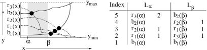
Figure 2. $r_{3}(x)$ lies above two blue curves at $x=\alpha$ but only lies above one blue curve at $x=\beta$. Subtraction reveals that $r_{3}(x)$ has one intersection in the slab $[\alpha,\beta]\times\mathbb{R}$.

To find a random red-blue intersection in $[\alpha,\beta]\times\mathbb{R}$, precompute the number $\kappa$ of red-blue intersections in $[\alpha,\beta]\times\mathbb{R}$. Pick a random integer between 1 and $\kappa$ and use the number of intersections stored for each red curve to locate the particular red curve $r_{i}(x)$ that is involved in the randomly selected intersection. By searching a persistent version of the reporting structure [24], $r_{i}(x)$’s $j$th red-blue intersection can be returned in $O(\log N+I(k))$ query time after $O(N\log N)$ preprocessing time. ∎

5. Geodesic Fréchet Algorithm

5.1. Computing One Cell’s Boundaries in $O(\log k)$ Time

A boundary of a free space cell is a horizontal (or vertical) line segment. This boundary can be associated with a funnel $\mathcal{F}_{p,\overline{cd}}$ that has a $\downarrow\uparrow$-bitonic distance function $F_{p,\ \overline{cd}}$ (cf. Lemma 2.1). Given $\varepsilon\geq 0$, computing the free space on a cell boundary requires finding the (at most two) values $t_{1}$, $t_{2}$ such that $F_{p,\ \overline{cd}}(t_{1})=F_{p,\ \overline{cd}}(t_{2})=\varepsilon$ (see Figure 3).

Figure 3. a & b) A funnel $\mathcal{F}_{p,\ \overline{cd}}$ is associated with a cell boundary and has a bitonic distance function $F_{p,\ \overline{cd}}$. c) The (at most two) values $t_{1}$, $t_{2}$ such that $F_{p,\ \overline{cd}}(t_{1})=F_{p,\ \overline{cd}}(t_{2})=\varepsilon$ define the free space on a cell boundary.

Lemma 5.1.

Both the minimum value of $F_{p,\ \overline{cd}}$ and the (at most two) values $t_{1}$, $t_{2}$ such that $F_{p,\ \overline{cd}}(t_{1})=F_{p,\ \overline{cd}}(t_{2})=\varepsilon$ can be found for any $\varepsilon\geq 0$ in $O(\log k)$ time (after preprocessing).

Proof Sketch.   After $O(k)$ shortest path preprocessing [13, 16], a binary search is performed on the $O(k)$ arcs of $F_{p,\ \overline{cd}}$ in $O(\log k)$ time. See our full paper [10] for details.∎

Corollary 5.2.

The free space on all four boundaries of a free space cell can be found in $O(\log k)$ time by computing $t_{1}$ and $t_{2}$ for each boundary.

5.2. Geodesic Fréchet Decision Problem

Theorem 5.3.

After preprocessing a simple polygon $P$ for shortest path queries in $O(k)$ time [13], the geodesic Fréchet decision problem for polygonal curves $A$ and $B$ inside $P$ can be solved for any $\varepsilon\geq 0$ in $O(N^{2}\log k)$ time and $O(k+N)$ space.

Proof 5.4.

Following the standard dynamic programming approach of [4], compute all cell boundaries in $O(N^{2}\log k)$ time (cf. Corollary 5.2), and propagate reachability information through all cells in $O(N^{2})$ time. $O(k)$ space is needed for the preprocessing structures of [13], and only $O(N)$ space is needed for dynamic programming if two rows of the free space diagram are stored at a time.

5.3. Geodesic Fréchet Optimization Problem

Let $\varepsilon^{*}$ be the minimum value of $\varepsilon$ such that the Fréchet decision problem returns true. That is, $\varepsilon^{*}$ equals the Fréchet distance $\delta_{F}(A,B)$. Parametric search is a technique commonly used to find $\varepsilon^{*}$ (see [3, 4, 9, 25]). The typical approach to find $\varepsilon^{*}$ is to sort all the cell boundary functions based on the unknown parameter $\varepsilon^{*}$. The comparisons performed during the sort guarantee that the result of the decision problem is known for all “critical values” [4] that could potentially define $\varepsilon^{*}$. Traditionally, such a sort operates on cell boundaries of constant complexity. The geodesic case is different because each cell boundary has $O(k)$ complexity. As a result, a straightforward parametric search based on sorting these values would require $O(kN^{2}\log kN)$ time even when using Cole’s [9] optimization.

We present a randomized algorithm with expected runtime $O(k+N^{2}\log kN\log N)$ and worst-case runtime $O(k+N^{3}\log kN)$. This algorithm is an order of magnitude faster than parametric search in the expected case.

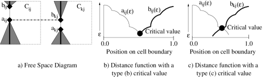
Figure 4. Critical values of the Fréchet distance

Each cell boundary has at most one free space interval (cf. Lemma 2.1). The upper boundary of this interval is a function $b_{ij}(\varepsilon)$, and the lower boundary of this interval is a function $a_{ij}(\varepsilon)$. See Figure 4a. The seminal work of Alt and Godau [4] defines three types of critical values that are useful for computing the exact geodesic Fréchet distance. There are exactly two type (a) critical values associated with distances between the starting points of $A$ and $B$ and the ending points of $A$ and $B$. Type (b) critical values occur $O(N^{2})$ times when $a_{ij}(\varepsilon)=b_{ij}(\varepsilon)$. See Figure 4b. Type (a) and (b) critical values occur $O(N^{2})$ times and are easily handled in $O(N^{2}\log k\log N)$ time. This process involves computing values in $O(N^{2}\log k)$ time, sorting in $O(N^{2}\log N)$ time, and running the decision problem in binary search fashion $O(\log N)$ times. Resolving the type (a) and (b) critical values as a first step will simplify the randomized algorithm for the type (c) critical values.

Alt and Godau [4] show that type (c) critical values occur when the position of $a_{ij}(\varepsilon)$ in cell $C_{ij}$ equals the position of $b_{kj}(\varepsilon)$ in cell $C_{kj}$ in the free space diagram. See Figure 4a. As $\varepsilon$ increases, by Lemma 2.1, $a_{ij}(\varepsilon)$ is $\downarrow$-monotone on the cell boundary and $b_{ij}(\varepsilon)$ is $\uparrow$-monotone (see Figure 4b). As illustrated in Figure 4c, $a_{ij}(\varepsilon)$ and $b_{kj}(\varepsilon)$ intersect at most once. This follows from the monotonicities of $a_{ij}(\varepsilon)$ and $b_{kj}(\varepsilon)$. Hence, there are $O(N^{2})$ intersections of $a_{ij}(\varepsilon)$ and $b_{kj}(\varepsilon)$ in row $j$ and a total of $O(N^{3})$ type (c) critical values over all rows. There are also $O(N^{2})$ intersections of $a_{ij}(\varepsilon)$ and $b_{ik}(\varepsilon)$ in column $i$ and a total of $O(N^{3})$ additional type (c) critical values over all columns.

Lemma 5.5.

The intersection of $a_{ij}(\varepsilon)$ and $b_{kl}(\varepsilon)$ can be found for any $\varepsilon\geq 0$ in $O(\log k)$ time after preprocessing.

Proof Sketch.   Build binary search trees for $a_{ij}(\varepsilon)$ and $b_{kl}(\varepsilon)$ and perform a binary search. See our full paper [10] for details.∎

Theorem 4.1 requires that all $a_{ij}(\varepsilon)$ and $b_{kl}(\varepsilon)$ are defined in the slab $[\alpha,\beta]\times\mathbb{R}$ that contains $\varepsilon^{*}$. Precomputing the type (a) and type (b) critical values of [4] shrinks the slab such that no left endpoint of any relevant $a_{ij}(\varepsilon)$, $b_{kl}(\varepsilon)$ appears in $[\alpha,\beta]\times\mathbb{R}$ when processing the type (c) critical values. In addition, $a_{ij}(\varepsilon)$, $b_{kl}(\varepsilon)$ can be extended horizontally so that no right endpoint appears in $[\alpha,\beta]\times\mathbb{R}$. These changes do not affect the asymptotic number of intersections and allow Theorem 4.1 to count and report type (c) critical values in $[\alpha,\beta]\times\mathbb{R}$.

The below randomized algorithm solves the geodesic Fréchet optimization problem in $O(k+N^{2}\log kN\log N)$ expected time. This is faster than the standard parametric search approach which requires $O(kN^{2}\log kN)$ time.

Randomized Optimization Algorithm

1. Precompute and sort all type (a) and type (b) critical values in $O(N^{2}\log kN)$ time (cf. Lemma 5.1). Run the decision problem $O(\log N)$ times to resolve these values and shrink the potential slab for $\varepsilon^{*}$ down to $[\alpha,\beta]\times\mathbb{R}$ in $O(N^{2}\log k\log N)$ time.

2. Count the number $\kappa_{j}$ of type (c) critical values for each row $j$ in the slab $[\alpha,\beta]\times\mathbb{R}$ using Theorem 4.1. Let $C_{j}$ be the resulting counting data structure for row $j$.

3. To achieve a fast expected runtime, pick a random intersection $\vartheta_{j}$ for each row using $C_{j}$. See Theorem 4.1.

4. To achieve a fast worst-case runtime, use $C_{j}$ to find the $a_{Mj}(\varepsilon)$ curve in each row that has the most intersections (see Theorem 4.1). Add all intersections in $[\alpha,\beta]\times\mathbb{R}$ that involve $a_{Mj}(\varepsilon)$ to a global pool $\mathcal{P}$ of unresolved critical values and delete $a_{Mj}(\varepsilon)$ from any future consideration.

5. Find the median $\Xi$ of the values in $\mathcal{P}$ in $O(N^{2})$ time using the standard median algorithm mentioned in [17]. Also find the median $\Psi$ of the $O(N)$ randomly selected $\vartheta_{j}$ in $O(N)$ time using a weighted median algorithm based on the number of critical values $\kappa_{j}$ for each row $j$.

6. Run the decision problem twice: once on $\Xi$ and once on $\Psi$. This shrinks the search slab $[\alpha,\beta]\times\mathbb{R}$ and at least halves the size of $\mathcal{P}$. Repeat steps 2 through 6 until all row-based type (c) critical values have been resolved.

7. Resolve all column-based type (c) critical values in the same spirit as steps 2 through 6 and return the smallest critical value that satisfied the decision problem as the value of the geodesic Fréchet distance.

Theorem 5.6.

The exact geodesic Fréchet distance between two polygonal curves $A$ and $B$ inside a simple bounding polygon $P$ can be computed in $O(k+N^{2}\log kN\log N)$ expected time and $O(k+N^{3}\log kN)$ worst-case time, where $N$ is the larger of the complexities of $A$ and $B$ and $k$ is the complexity of $P$. $O(k+N^{2})$ space is required.

Proof 5.7.

Preprocess $P$ once for shortest path queries in $O(k)$ time [13]. In the expected case, each execution of the decision problem will eliminate a constant fraction of the remaining type (c) critical values due to the proof of Quicksort’s expected runtime and the median of medians approach for $\Psi$. Consequently, the expected number of iterations of the algorithm is $O(\log N^{3})=O(\log N)$.

In the worst-case, each of the $O(N)$ $a_{ij}(\varepsilon)$ in a row will be picked as $a_{Mj}(\varepsilon)$. Therefore, each row can require at most $O(N)$ iterations. Since all rows are processed each iteration, the entire algorithm requires at most $O(N)$ iterations for row-based critical values. By a similar argument, column-based critical values also require at most $O(N)$ iterations.

The size of the pool $\mathcal{P}$ is expressed by the inequality $S(x)\leq\frac{S(x-1)+O(N^{2})}{2}$, where $x$ is the current step number, and $S(0)=0$. Intuitively, each step adds $O(N^{2})$ values to $\mathcal{P}$ and then at least half of the values in $\mathcal{P}$ are always resolved using the median $\Xi$. It is not difficult to show that $S(x)\in O(N^{2})$ for any step number $x$.

Each iteration of the algorithm requires intersection counting and intersection calculations for $O(N)$ rows (or columns) at a cost of $O(N^{2}\log kN)$ time. In addition, the global pool $\mathcal{P}$ has its median calculated in $O(N^{2})$ time, and the decision problem is executed in $O(N^{2}\log k)$ time. Consequently, the expected runtime is $O(k+N^{2}\log kN\log N)$ and the worst-case runtime is $O(k+N^{3}\log kN)$ including $O(k)$ preprocessing time [13] for geodesics. The preprocessing structures use $O(k)$ space that must remain allocated throughout the algorithm, and the pool $\mathcal{P}$ uses $O(N^{2})$ additional space.

Although the exact non-geodesic Fréchet distance is normally found in $O(N^{2}\log N)$ time using parametric search (see [4]), parametric search is often regarded as impractical because it is difficult to implement and involves enormous constant factors [9]. To the best of our knowledge, the randomized algorithm in section 5.3 provides the first practical alternative to parametric search for solving the exact non-geodesic Fréchet optimization problem in $\mathbb{R}^{l}$.

Theorem 5.8.

The exact non-geodesic Fréchet distance between two polygonal curves $A$ and $B$ in $\mathbb{R}^{l}$ can be computed in $O(N^{2}\log^{2}N)$ expected time, where $N$ is the larger of the complexities of $A$ and $B$. $O(N^{2})$ space is required.

Proof 5.9.

The argument is very similar to the proof of Theorem 5.6. The main difference is that non-geodesic distances can be computed in $O(1)$ time (instead of $O(\log k)$ time).

6. Geodesic Fréchet Distance in a Polygonal Domain with Obstacles

Consider the real-life situation of a person walking a dog in a park. If the person and dog walk on opposite sides of a group of trees, then the leash must go around the trees. More formally, suppose the two polygonal curves $A$ and $B$ lie in a planar polygonal domain $\mathcal{D}$ [19] of complexity $k$. The leash is required to change continuously, i.e., it must stay inside $\mathcal{D}$ and may not pass through or jump over an obstacle. It may, however, cross itself. Let $\delta_{C}$ be the geodesic Fréchet distance for this scenario when the leash length is measured geodesically.

Due to the continuity of the leash’s motion, the free space inside a geodesic cell is represented by an hourglass – just as it was for the geodesic Fréchet distance inside a simple polygon. Hence, free space in a cell is $x$-monotone, $y$-monotone, and connected (cf. Lemma 3.1), and reachability information can be propagated through a cell in constant time.

The main task in computing $\delta_{C}$ is to construct all cell boundaries. Once the cell boundaries are known, the decision and optimization problems can be solved by the algorithms for the geodesic Fréchet distance inside a simple polygon (cf. Theorems 5.3 and 5.6). We use Hershberger and Snoeyink’s homotopic shortest paths algorithm [16] to incrementally construct all cell boundary funnels needed to compute $\delta_{C}$. To use the homotopic algorithm, the polygonal domain $\mathcal{D}$ should be triangulated in $O(k\log k)$ time [19], and all obstacles should be replaced by their vertices. A shortest path map [19] can find an initial geodesic leash $L_{I}$ between the start points of the polygonal curves $A$ and $B$ in $O(k\log k)$ time.

Lemma 6.1.

Given the initial leash for the bottom-left corner of a $\delta_{C}$-cell $\mathcal{C}$, all four funnel boundaries of $\mathcal{C}$ and the initial leashes for cells adjacent to $\mathcal{C}$ can be computed in $O(k)$ time.

Proof 6.2.

The funnels representing cell boundaries are constructed incrementally. The idea is to extend the initial leash into a homotopic “sketch” that describes how the shortest path should wind through the obstacles and then to “snap” this sketch into a shortest path (see Figures 5a and 5b).

Figure 5. a) A funnel for a $\delta_{C}$-cell can be found by extending a cell’s initial leash along one segment to create a path sketch and then b) snapping this sketch into a homotopic shortest path. c) A funnel $\mathcal{F}_{o,\ \overline{cd}}$ has $O(kN)$ complexity, but the distance function $F_{o,\ \overline{cd}}$ has only $O(k)$ complexity because $d(o,p)$ is a constant.

Homotopic shortest paths have increased complexity over normal shortest paths because they can loop around obstacles. For example, if the person walks in a triangular path around all the obstacles, then the leash follows a homotopic shortest path that can have $O(k)$ complexity in a single cycle around the obstacles. By repeatedly winding around the obstacles $O(N)$ times, a path achieves $O(kN)$ complexity.

To avoid spending $O(kN)$ time per cell, we extend a previous homotopic shortest path into a sketch by appending a single line segment to the previous path (see Figure 5a). Adding this single segment can unwind at most one loop over a subset of obstacles, so only the most recent $O(k)$ vertices of the sketch will need to be updated when the sketch is snapped into the true homotopic shortest path. A turning angle is used to identify these $O(k)$ vertices by backtracking on the sketch until the angle is at least $2\pi$ different from the final angle.

Putting all this together, a boundary for a free space cell can be computed in $O(k)$ time by starting with an initial leash $L_{I}$ of $O(kN)$ complexity, constructing a homotopic sketch by appending a single segment to $L_{I}$, backtracking with a turning angle to find $O(k)$ vertices that are eligible to be changed, and finally “snapping” these $O(k)$ vertices to the true homotopic shortest path using Hershberger and Snoeyink’s algorithm [16]. The result is a funnel that describes one cell boundary.

By extending $L_{I}$ in four combinatorially distinct ways, all four cell boundaries can be defined. Specifically, we can extend $L_{I}$ along the current $\overline{ab}\in A$ segment to form the first funnel or along the $\overline{cd}\in B$ segment to form the second funnel. The third funnel is created by extending $L_{I}$ along $\overline{ab}\in A$ and then $\overline{cd}\in B$. The fourth funnel is created by extending $L_{I}$ along $\overline{cd}\in B$ and then $\overline{ab}\in A$. These cell boundaries conveniently define the initial leash for cells that are adjacent to $\mathcal{C}$.

Theorem 6.3.

The $\delta_{C}$ decision problem can be solved in $O(kN^{2})$ time and $O(k+N)$ space.

Proof 6.4.

Each cell boundary is a funnel $\mathcal{F}_{o,\ \overline{cd}}$ with $O(kN)$ complexity [11]. However, this high complexity is a result of looping over obstacles, and most of these points do not affect the funnel’s distance function $F_{o,\ \overline{cd}}$. As illustrated in Figure 5c, $F_{o,\ \overline{cd}}$ has only $O(k)$ complexity because only vertices $\pi(p,c)\cup\pi(p,d)$ contribute arcs to $F_{o,\ \overline{cd}}$.

Construct all cell boundary funnels in $O(kN^{2})$ time (cf. Lemma 6.1), intersect each funnel’s distance function with $y=\varepsilon$ in $O(N^{2}\log k)$ time, and propagate reachability information in $O(N^{2})$ time. Only $O(k+N)$ space is needed for dynamic programming when storing only two rows at a time.

Theorem 6.5.

The $\delta_{C}$ optimization problem can be solved in $O(kN^{2}+N^{2}\log kN\log N)$ expected time and $O(kN^{2})$ space.

Proof 6.6.

The $\delta_{C}$ optimization problem can be solved using red-blue intersections. $O(\log N)$ steps are performed in the expected case by Theorem 5.6. Each step has to perform intersection counting in $O(N^{2}\log kN)$ time and solve the decision problem. If the funnels are precomputed in $O(kN^{2})$ time and space, then the decision problem can be solved in $O(N^{2}\log k)$ time. Hence, after $O(kN^{2})$ time and space preprocessing, $\delta_{C}$ can be found in $O(\log N)$ expected steps where each step takes $O(N^{2}\log kN)$ time.

7. Geodesic Hausdorff Distance

Hausdorff distance is a similarity metric commonly used to compare sets of points or sets of line segments. The directed geodesic Hausdorff distance can be formally defined as $\tilde{\delta}_{H}(A,B)=\ \sup_{a\in A}\inf_{b\in B}d(a,b)$, where $A$ and $B$ are sets and $d(a,b)$ is the geodesic distance between $a$ and $b$ (see [4, 5]). The undirected geodesic Hausdorff distance is the larger of the two directed distances: $\delta_{H}(A,B)=\max(\tilde{\delta}_{H}(A,B),\ \tilde{\delta}_{H}(B,A))$.

Theorem 7.1.

$\delta_{H}(A,B)$ for point sets $A,B$ inside a simple polygon $P$ can be computed in $O((k+N)\log(k+N))$ time and $O(k+N)$ space, where $N$ is the larger of the complexities of $A$ and $B$ and $k$ is the complexity of $P$. If $A$ and $B$ are sets of line segments, $\delta_{H}(A,B)$ can be computed in $O(kN^{2}\alpha(kN)\log kN)$ time and $O(kN\alpha(kN)\log kN)$ space.

Proof Sketch.   A geodesic Voronoi diagram [22] finds nearest neighbors when $A$ and $B$ are point sets. When $A$ and $B$ are sets of line segments, all nearest neighbors for a line segment can be found by computing a lower envelope [1] of $O(N)$ hourglass distance functions. The largest nearest neighbor distance over all line segments is $\delta_{H}(A,B)$. ∎

8. Conclusion

To compute the geodesic Fréchet distance between two polygonal curves inside a simple polygon, we have proven that the free space inside a geodesic cell is $x$-monotone, $y$-monotone, and connected. By extending the shortest path algorithms of [13, 16], the boundaries of a single free space cell can be computed in logarithmic time, and this leads to an efficient algorithm for the geodesic Fréchet decision problem.

A randomized algorithm based on red-blue intersections solves the geodesic Fréchet optimization problem in lieu of the standard parametric search approach. The randomized algorithm is also a practical alternative to parametric search for the non-geodesic Fréchet distance in arbitrary dimensions.

We can compute the geodesic Fréchet distance between two polygonal curves $A$ and $B$ inside a simple bounding polygon $P$ in $O(k+N^{2}\log kN\log N)$ expected time, where $N$ is the larger of the complexities of $A$ and $B$ and $k$ is the complexity of $P$. In the expected case, the randomized optimization algorithm is an order of magnitude faster than a straightforward parametric search that uses Cole’s [9] optimization to sort $O(kN^{2})$ values.

The geodesic Fréchet distance in a polygonal domain with obstacles enforces a homotopy on the leash. It can be computed in the same manner as the geodesic Fréchet distance inside a simple polygon after computing cell boundary funnels using Hershberger and Snoeyink’s homotopic shortest paths algorithm [16]. Future work could attempt to compute these funnels in $O(\log k)$ time instead of $O(k)$ time. The geodesic Hausdorff distance for point sets inside a simple polygon can be computed using geodesic Voronoi diagrams. The geodesic Hausdorff distance for line segments can be computed using lower envelopes; future work could speed up this algorithm by developing a geodesic Voronoi diagram for line segments.

References

- [1] P. K. Agarwal and M. Sharir. Davenport–Schinzel sequences and their geometric applications. Technical Report Technical report DUKE–TR–1995–21, 1995.
- [2] P. K. Agarwal and M. Sharir. Efficient algorithms for geometric optimization. ACM Comput. Surv., 30(4):412–458, 1998.
- [3] P. K. Agarwal, M. Sharir, and S. Toledo. Applications of parametric searching in geometric optimization. volume 17, pages 292–318, Duluth, MN, USA, 1994. Academic Press, Inc.
- [4] H. Alt and M. Godau. Computing the Fréchet distance between two polygonal curves. International Journal of Computational Geometry and Applications, 5:75–91, 1995.
- [5] H. Alt, C. Knauer, and C. Wenk. Comparison of distance measures for planar curves. Algorithmica, 38(1):45–58, 2003.
- [6] S. Bespamyatnikh and M. Segal. Selecting distances in arrangements of hyperplanes spanned by points. volume 2, pages 333–345, September 2004.
- [7] K. Buchin, M. Buchin, and C. Wenk. Computing the Fréchet distance between simple polygons in polynomial time. SoCG: 22nd Symposium on Computational Geometry, pages 80–87, 2006.
- [8] E. W. Chambers, É. C. de Verdière, J. Erickson, S. Lazard, F. Lazarus, and S. Thite. Walking your dog in the woods in polynomial time. 17th Fall Workshop on Computational Geometry, 2007.
- [9] R. Cole. Slowing down sorting networks to obtain faster sorting algorithms. J. ACM, 34(1):200–208, 1987.
- [10] A. F. Cook IV and C. Wenk. Geodesic Fréchet and Hausdorff distance inside a simple polygon. Technical Report CS-TR-2007-004, University of Texas at San Antonio, August 2007.
- [11] C. A. Duncan, A. Efrat, S. G. Kobourov, and C. Wenk. Drawing with fat edges. Int. J. Found. Comput. Sci., 17(5):1143–1164, 2006.
- [12] A. Efrat, L. J. Guibas, S. Har-Peled, J. S. B. Mitchell, and T. M. Murali. New similarity measures between polylines with applications to morphing and polygon sweeping. Discrete & Computational Geometry, 28(4):535–569, 2002.
- [13] L. J. Guibas and J. Hershberger. Optimal shortest path queries in a simple polygon. J. Comput. Syst. Sci., 39(2):126–152, 1989.
- [14] L. J. Guibas, J. Hershberger, D. Leven, M. Sharir, and R. E. Tarjan. Linear time algorithms for visibility and shortest path problems inside simple polygons. pages 1–13, 1986.
- [15] L. J. Guibas, J. Hershberger, D. Leven, M. Sharir, and R. E. Tarjan. Linear-time algorithms for visibility and shortest path problems inside triangulated simple polygons. Algorithmica, 2:209–233, 1987.
- [16] J. Hershberger. A new data structure for shortest path queries in a simple polygon. Inf. Process. Lett., 38(5):231–235, 1991.
- [17] J. Komlós, Y. Ma, and E. Szemerédi. Matching nuts and bolts in O(n log n) time. SODA: 7th ACM-SIAM Symposium on Discrete Algorithms, pages 232–241, 1996.
- [18] A. Maheshwari and J. Yi. On computing Fréchet distance of two paths on a convex polyhedron. EWCG 2005, pages 41–4, 2005.
- [19] J. S. B. Mitchell. Geometric shortest paths and network optimization. Handbook of Computational Geometry, 1998.
- [20] J. S. B. Mitchell, D. M. Mount, and C. H. Papadimitriou. The discrete geodesic problem. SIAM J. Comput., 16(4):647–668, 1987.
- [21] L. Palazzi and J. Snoeyink. Counting and reporting red/blue segment intersections. CVGIP: Graph. Models Image Process., 56(4):304–310, 1994.
- [22] E. Papadopoulou and D. T. Lee. A new approach for the geodesic Voronoi diagram of points in a simple polygon and other restricted polygonal domains. Algorithmica, 20(4):319–352, 1998.
- [23] G. Rote. Computing the Fréchet distance between piecewise smooth curves. Technical Report ECG-TR-241108-01, May 2005.
- [24] N. Sarnak and R. E. Tarjan. Planar point location using persistent search trees. Commun. ACM, 29(7):669–679, 1986.
- [25] R. van Oostrum and R. C. Veltkamp. Parametric search made practical. SoCG: 18th Symposium on Computational Geometry, pages 1–9, 2002.
- [26] C. Wenk, R. Salas, and D. Pfoser. Addressing the need for map-matching speed: Localizing global curve-matching algorithms. 18th Int’l Conf. on Sci. and Statistical Database Mgmt (SSDBM), pages 379–388, 2006.