Diagrammatic Monte Carlo

Abstract

Diagrammatic Monte Carlo (DiagMC) is a numeric technique that allows one to calculate quantities specified in terms of diagrammatic expansions, the latter being a standard tool of many-body quantum statistics. The sign problem that is typically fatal to Monte Carlo approaches, appears to be manageable with DiagMC. Starting with a general introduction to the principles of DiagMC, we present a detailed description of the DiagMC scheme for interacting fermions (Hubbard model), as well as the first illustrative results for the equations of state.

1 Introduction. General Principles

Diagrammatic expansion (Feynman diagrams) is a powerful generic tool of quantum statistics Fetter_Walecka . Mathematically, diagrammatic expansion—for some relevant quantity, $Q$, usually a Green’s function—is a series of integrals with an ever increasing number of integration variables,

$$Q(y)\,=\,\sum_{m=0}^{\infty}\sum_{\xi_{m}}\int\mathcal{D}(\xi_{m},y,x_{1},\ldots,x_{m})\,dx_{1}\cdots dx_{m}\;.$$ (1)

Here $y$ is a set of parameters which the quantity $Q$ can depend on, $\xi_{m}$ indexes different terms of the same order $m$ (the term $m=0$ is understood as a function of $y$ only), and the $x$’s are the integration variables. Structures similar to Eq. (1) originate from perturbative expansions of the quantum-statistical averages, in which case the functions $\mathcal{D}$ can be represented by Feynman diagrams/graphs, with the graph lines standing for either Green’s functions (propagators) $G$ or interaction potentials $U$, so that the whole diagram encodes a certain product of $G$’s and $U$’s. It will be essential for our purposes to approach the integrations in Eq. (1) in the same way as the diagram order $m$ and its topology when defining the notion of a diagram, in contrast to analytic treatments where integrations are included into the definition of $\mathcal{D}$.

Diagrammatic Monte Carlo (DiagMC) DiagMC is a technique that allows one to simulate quantities specified in terms of a diagrammatic series. In a broad sense, it is a set of simple generic prescriptions for organizing a systematic-error-free Metropolis-Rosenbluth-Teller type process that samples the series (1) without explicitly performing integrations over the internal variables in each particular term. The rules are as follows.

The function $Q(y)$ is interpreted as a distribution function for the variable(s) $y$. The statistical interpretation of Eq. (1) suggests calculating $Q(y)$ by a Markov-chain process which samples diagrams stochastically. The value of $\mathcal{D}$ plays the role of the statistical weight of the diagram (i.e., the probability with which the diagram is generated). More precisely, to deal with sign-alternating series, one writes $\mathcal{D}$ as a product of its absolute value $|\mathcal{D}|$, which determines the statistical weight of the diagram, and the sign function $s_{\mathcal{D}}=\pm 1$, which contributes to the statistics for $Q$ each time the term $\mathcal{D}$ is generated. Since contributions of different $m$-th order diagrams are of the same order of magnitude and their number grows factorially with $m$, the combined $m$-th order contribution to $Q$ is the result of nearly complete cancellation of the diagrams of different sign. This is the notorious sign problem (see, e.g., Troyer ). In our case, it causes an exponential scaling of the computation time with the maximum diagram order, making it impossible to obtain sensible results at large $m$. At this point one faces the problem of extrapolating the answer to the $m\to\infty$ limit. To make matters worse, the series may be asymptotic/divergent. For this reason, the use of resummation techniques fermipolaron is a crucial ingredient of DiagMC (see Secs. 4, 5).

Though DiagMC has to confront the sign problem, just like other exact techniques (e.g., the dynamical cluster algorithms DCA ), it has an important advantage: it works immediately in the thermodynamic limit, and is not subject to the exponential scaling of the computational complexity with the system or cluster volume. DiagMC also has a potential for vast improvements in efficiency by using standard tricks of the analytic diagrammatic approach, developed to reduce the number of diagrams calculated explicitly term-by-term by self-consistently taking into account chains of repeating parts as, e.g., in the Dyson equation Fetter_Walecka . These ideas are the essence of the Bold Monte Carlo scheme introduced in Ref. bmc and successfully applied to the Fermi-polaron problem in Ref. fermipolaron . In Sec. 4, we describe the basic steps in this direction for DiagMC, such as the use of bold propagators.

The stochastic sampling of $Q(y)$ consists of a number of elementary sub-processes (or updates) falling into two qualitatively different classes: (I) updates which do not change the number of continuous variables (they change the values of variables in $\mathcal{D}$, but not the form of the function itself), and (II) updates which change the structure of $\mathcal{D}$. The processes of class I are rather straightforward, being identical to those of simulating a given continuous distribution $|\mathcal{D}(\xi_{m},y,x_{1},\ldots,x_{m})|$ of the variables $x_{1},\ldots,x_{m}$.

The crucial part is played by type-II updates, arranged to form complementary pairs with the detailed balance condition Metropolis satisfied in each pair. Let $\cal A$ transform the diagram ${\mathcal{D}}(\xi_{m},y,x_{1},\ldots,x_{m})$ into $\mathcal{D}(\xi_{m+n},y,x_{1},\ldots,x_{m+n})$, and, correspondingly, its counterpart $\cal B$ performs the inverse transformation. For the new variables we introduce a vector notation: ${\vec{x}}=\{x_{m+1},\ldots,x_{m+n}\}$. The first step in $\cal A$ consists of selecting some type of diagram transformation and proposing $\vec{x}$ which is generated from a certain probability distribution $W(\vec{x})$. The form of $W(\vec{x})$ is arbitrary, but to render the algorithm most efficient, it is desirable that $W(\vec{x})$ is (i) of a simple analytic form with known normalization, and (ii) close to the actual statistics of $\vec{x}$ in the final diagram. The second step consists of accepting the proposal with probability, $P_{\mbox{\scriptsize add}}(\vec{x})$. In $\cal B$ one simply accepts the proposal for removing the variables $\vec{x}$ with the probability $P_{\mbox{\scriptsize rem}}(\vec{x})$. The pair of complementary sub-processes is balanced if the following equality is fulfilled DiagMC :

$$P_{\mbox{\scriptsize add}}(\vec{x})\>=\>\min\{R(\vec{x})/W(\vec{x}),1\}\;,$$ (2)

$$P_{\mbox{\scriptsize rem}}(\vec{x})\>=\>\min\{W(\vec{x})/R(\vec{x}),1\}\;,$$ (3)

where

$$R(\vec{x})\,=\,(p_{\cal B}/p_{\cal A})\,|\mathcal{D}(\xi_{m+n},y,x_{1},\ldots,x_{m},{\vec{x}})/\mathcal{D}(\xi_{m},y,x_{1},\ldots,x_{m})|\;,$$ (4)

with $p_{\cal A}$ and $p_{\cal B}$ being the probabilities of addressing the sub-processes $\cal A$ and $\cal B$. [Often, $p_{\cal A}\neq p_{\cal B}$ is a natural choice.] The above protocol is a straightforward generalization of the standard approach Metropolis ; Hastings to the sampling of functions with a variable number of continuous arguments.

Generally speaking, the set of DiagMC updates is specific for a given type of the diagrammatic expansion, being sensitive to both the topology and the representation (say, momentum or coordinate) of the diagrams. The updating strategy can be rendered more/less sophisticated, depending on what is being optimized: the simplicity or the efficiency. Examples of particular DiagMC schemes can be found in Refs. DiagMC ; fermipolaron ; Mishchenko ; Burovski_01 ; Burovski_06 .

In this work, we consider an interacting many-body Fermi system and work with diagrams in the imaginary-time–momentum representation. We employ a sophisticated (at first glance) updating scheme based on the worm algorithm idea worm when updating flexibility and efficiency are achieved by extending the configurational space (in our case, the space of allowed diagrams). As far as we know, the algorithm being presented is the first application of the DiagMC method to connected many-body Feynman diagrams.

Perturbative expansions in the interaction are often divergent. Dyson gave a simple physical argument leading to a sufficient condition for an expansion series to diverge: if changing the sign (or phase) of some parameter $\gamma$ implies an abrupt change of the physical state (e.g., the change of symmetry, or an instability), then $\gamma=0$ is the point of non-analyticity and the expansion in powers of $\gamma$ is a priori divergent Dyson . In particular, this means the diagrammatic expansion with respect to the interaction in continuous space is divergent for both bosons and fermions, since both systems collapse at negative (on average) interaction. Obviously, the opposite is not necessarily true—that is the absence of singularity in the aforementioned sense does not guarantee analyticity (and thus convergence at small enough $\gamma$)—but a different reason for a series to be non-analytic (and thus divergent at arbitrarily small $\gamma$) should be rather exotic. Therefore, we shall rely on the physical picture to predict the analytic properties of the series at $\gamma\to 0$.

However, the real power of the analytic diagrammatic technique lies in the possibility of reducing infinite sums of diagrams (no matter convergent or divergent) to simple integral equations, e.g., the Dyson equation. In addition to that, for divergent asymptotic series one can employ generalized resummation schemes to obtain the answer outside of the series convergence radius. Finally, when the resummation trick fails, the series can be analyzed using approximate (biased) methods, which assume a certain function behind the series. An example of the successful application of the resummation method to a divergent sign alternating series for polarons can be found in Ref. fermipolaron . In this work we demonstrate that the DiagMC method is a viable approach to study interacting many-body systems. Even moderate success in this direction is extremely important since other Monte Carlo approaches face a severe sign problem before the fully controlled extrapolation to the thermodynamic limit can be done.

2 Model and Diagrams

In what follows we discuss the Fermi-Hubbard model,

$$H\,=\,\sum_{\mathbf{k},\sigma}\,(\varepsilon_{\mathbf{k}}-\mu_{\sigma})\,a^{\dagger}_{\sigma\mathbf{k}}a^{\phantom{\dagger}}_{\sigma\mathbf{k}}\,+\,U\sum_{\mathbf{r}}\,n_{\uparrow\mathbf{r}}\,n_{\downarrow\mathbf{r}}\;.$$ (5)

Here $a^{\dagger}_{\sigma\mathbf{k}}$ is the fermion creation operator with the quasi-momentum ${\bf k}$ lying in the first Brillouin zone, $n_{\sigma\mathbf{r}}=a^{\dagger}_{\sigma\mathbf{r}}a^{\phantom{\dagger}}_{\sigma\mathbf{r}}$, $\sigma=\uparrow\;,\downarrow$ is the spin projection, and $\mathbf{r}$ is the integer radius vector on the d-dimensional lattice. The lattice dispersion is given by $\varepsilon_{\mathbf{k}}=-2t\sum_{\alpha=1}^{d}{\rm cos}({\rm k}_{\alpha}a)$, with $a$ and $t$ being the lattice spacing and the hopping amplitude, respectively; $\mu_{\sigma}$ is the chemical potential for the component $\sigma$, and $U$ is the on-site interaction strength. Units are chosen such that $a$ and $t$ are equal to unity.

[width=0.3keepaspectratio=true]f1.eps

Figure 1: The diagram structural element. The dashed vertical line represents the interaction potential. The upper (lower) solid lines represent spin-up (spin-down) fermionic propagators.

We utilize the standard Matsubara diagrammatic technique Fetter_Walecka . The diagrams consist of (vertical) dashed lines standing for the pair interaction potential $U$ and solid lines representing particle propagators $G^{(0)}$ (see Fig. 1). We adopt a convention that the imaginary-time axis is horizontal, and is directed from right to left. Since in our case there are no interactions within one and the same component, we require that the upper (lower) end of each dashed line corresponds to the spin-up (spin-down) component. With this rule, the spin-up lines are distinguished from spin-down ones without explicit labeling.

A free fermionic propagator $G^{(0)}_{\sigma}(\mathbf{k},\,\tau=\tau_{2}-\tau_{1})$ associated with each particle line running from $\tau_{1}$ to $\tau_{2}$ is defined by

$$G^{(0)}_{\sigma}(\mathbf{k},\tau)\,=\,\left\{\begin{array}[]{ll}-e^{-(\varepsilon_{\mathbf{k}}-\mu_{\sigma})\tau}(1-n^{(0)}_{\sigma\mathbf{k}})\,,&\textrm{~{}~{}if $\tau>0$}\;,\\ +e^{-(\varepsilon_{\mathbf{k}}-\mu_{\sigma})\tau}n^{(0)}_{\sigma\mathbf{k}}\,,&\textrm{~{} if $\tau<0$}\;,\\ \end{array}\right.$$ (6)

with $n^{(0)}_{\sigma\mathbf{k}}=\left[1+e^{\beta(\varepsilon_{\mathbf{k}}-\mu_{\sigma})}\right]^{-1}$ being the occupation of the state $(\sigma,\mathbf{k})$ at inverse temperature $\beta$ for free fermions on the lattice. A Green’s function with equal time variables (a closed fermion loop) is understood as $G^{(0)}_{\sigma}(\mathbf{k},\,\tau=-0)$. To obtain the right weight and sign, one also has to ascribe the factor $(-1)^{N+N_{l}}/(2\pi)^{Nd}$ to each diagram of order $N$, with $N_{l}$ being the number of closed fermion loops and $d$ the dimensionality of the problem.

All the physical information we will need is contained in the self-energy $\Sigma_{\sigma}$ Fetter_Walecka . In analytic treatments, it is convenient to have $\Sigma_{\sigma}$ in the momentum–imaginary-frequency representation, so that the Green’s function is obtained from the Dyson equation by simple algebra:

$$\left[G_{\sigma}(\mathbf{p},\xi)\right]^{-1}\,=\,\left[G^{(0)}_{\sigma}(\mathbf{p},\xi)\right]^{-1}-\Sigma_{\sigma}(\mathbf{p},\xi)\;.$$ (7)

Numerically, we find it more appropriate to work in the momentum–imaginary-time representation, to avoid dealing with poles. This does not create a problem with finding $G_{\sigma}(\mathbf{p},\xi)$, since $\Sigma_{\sigma}(\mathbf{p},\xi)$ is readily obtained from $\Sigma_{\sigma}(\mathbf{p},\tau)$ by a (fast) Fourier transform.

The class of diagrams contributing to $\Sigma_{\sigma}(\mathbf{p},\tau)$ is defined by the following requirements: (i) Each diagram has two special vertices having one open fermionic end. These vertices are separated by the time interval $\tau$ and their open ends have the same spin projection $\sigma$ and momentum $\mathbf{p}$ which enters the diagram at one open end and exits at the other. (ii) Each diagram is connected. (iii) Each diagram is irreducible, i.e., it can not be split into two disconnected parts by cutting only a single fermionic line.

3 Updates

For the sake of algorithmic elegance, we choose to work with closed-loop diagrams that (formally) have no free ends. To collect statistics for $\Sigma$ in this representation, we fix one propagator, say going from vertex 1 to vertex 2, and set its value to $1$. Below, we refer to this special propagator as ‘measuring’ propagator. Then, if the propagator’s momentum is $\mathbf{p}$ and the vertices have times $\tau_{1},\tau_{2}$ respectively, we are measuring $\Sigma(\mathbf{p},\tau_{1}-\tau_{2})$. Note that $\Sigma(\mathbf{p},\tau)$ is an anti-periodic function of $\tau$ (with $\tau=\tau_{1}-\tau_{2}$), so we can restrict ourselves to collecting statistics for $0<\tau<\beta$. For a given diagram, changing the measuring propagator—without changing the diagram structure—is straightforwardly done by the Swap update.

Swap. The update swaps the measuring propagator with one of the regular propagators. The new measuring propagator is chosen at random, and its value is set to $1$. Correspondingly, the physical value of the old measuring propagator is restored, so that it becomes just a regular propagator.

Assume that the initial measuring propagator has to be replaced with $G^{(0)}_{\alpha}(\mathbf{p},\tau)$, after we swap it with the propagator $G^{(0)}_{\beta}(\mathbf{p}^{\prime},\tau^{\prime})$. The acceptance ratio is given by

$$P_{{\rm swap}}\,=\,|G^{(0)}_{\alpha}(\mathbf{p},\tau)/G^{(0)}_{\beta}(\mathbf{p}^{\prime},\tau^{\prime})|\;.$$ (8)

The problem of generating diagrams for $\Sigma$ consists of two main tasks: one should be able to (i) change the structure of the diagrams, and (ii) make sure that the momentum conservation is satisfied in every vertex. We develop a scheme that fulfills these tasks by performing only local updates of the diagram. The idea—in the spirit of the worm algorithm—is to introduce non-physical diagrams in which momentum conservation is violated in some special vertices (called worms). The smallest required number of such vertices is two. All updates changing the topology of the diagram involve worms. When worms are deleted from the diagram we return to the physical subspace.

To be specific, we introduce the following notation. One of the three-point vertices in which momentum conservation is violated, if any, is labeled $\mathcal{I}$. There is an excess momentum $\vec{\delta}$ associated with $\mathcal{I}$, which is defined as the difference between the incoming and the outgoing momenta in this vertex (see Fig. 2). If present, $\mathcal{I}$ always has one, and only one, conjugate vertex $\mathcal{M}$ with an excess momentum $-\vec{\delta}$, as shown in Fig. 2. Clearly, the distinction between $\mathcal{I}$ and $\mathcal{M}$ is merely conventional, since replacing $\vec{\delta}$ with $-\vec{\delta}$ interchanges $\mathcal{I}$ and $\mathcal{M}$. There is an important property of the two worms: once some path from $\mathcal{I}$ to $\mathcal{M}$ is known, one can simply remove the worms by propagating the excess momentum $\vec{\delta}$ along the path.

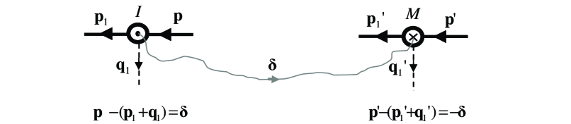
Figure 2: Worms. Graphically, we can picture the worms as vertices with conserving momentum, by connecting the two with an extra line (thread) that transports the momentum $\vec{\delta}$ from $\mathcal{I}$ to $\mathcal{M}$. The indistinguishability of $\mathcal{I}$ and $\mathcal{M}$ is seen from the fact that swapping the labels $\mathcal{I}$ and $\mathcal{M}$, and replacing $\vec{\delta}\to-\vec{\delta}$ yields the same original diagram.

We proceed now with the description of the updates. The Create/Delete pair switches between the physical and non-physical (worm) diagrammatic spaces by creating/deleting $\mathcal{I}$, $\mathcal{M}$. Its role is also to update the diagram’s momenta. The Add/Remove pair changes the diagram order. In these updates, we add (remove) a vertex and delete (create) $\mathcal{I}$, $\mathcal{M}$ on different spin components at the same time. The self-complementary updates Move and Reconnect are responsible for moving the worms in the diagram and changing its topology, respectively.

Create. This update is possible only—being rejected otherwise—when we are in the physical sector ($\Sigma$-sector), that is when $\mathcal{I,M}$ are absent. We introduce $\mathcal{I,M}$ by selecting a propagator (line) at random and adding a momentum $\vec{\delta}$ to it (see Fig. 3). [Similarly, $\mathcal{I}$ and $\mathcal{M}$ can be also created on the two vertices of an interaction line.]

Creating two worms takes the diagram from the $\Sigma$-sector to the non-physical $W$-sector. We define the $W$-diagram weight by exactly the same rules as for physical ones up to an arbitrary numeric factor, so that the acceptance ratio for Create is

$$P_{\rm create}\,=\,2N\,C_{N}\,G^{(0)}(\mathbf{p}+\vec{\delta},\tau)/(2\pi)^{d}W(\vec{\delta})~{}G^{(0)}(\mathbf{p},\tau)\;,$$ (9)

where $2N$ is the total number of propagators (including the measuring propagator) and $W(\vec{\delta})$ is the normalized distribution from which $\vec{\delta}$ is drawn. The variable $C_{N}$ is an extra weighing factor which is assigned to a diagram of order $N$ whenever the worm is present. To make transitions between the $\Sigma$- and $W$-sectors efficiently, we choose $\,C_{N}\,=\,C/2N$, where $C$ is a constant.

The simplest choice for $W(\vec{\delta})$ is to assume a uniform distribution in the first Brillouin zone, $W(\vec{\delta})=1/(2\pi)^{d}$. Since $\mathcal{I}$ and $\mathcal{M}$ are indistinguishable, we find it convenient to require that the leftmost worm is labeled $\mathcal{I}$, and the rightmost one $\mathcal{M}$ (see Fig. 3).

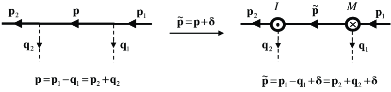
Figure 3: Create update.

The rest of the updates (except for Remove) apply only—being automatically rejected otherwise—when $\mathcal{I,M}$ are present.

Delete. Here, we first check if $\mathcal{I}$ and $\mathcal{M}$ are connected by a single line and proceed only if they are. We propose to remove $\mathcal{I}$ and $\mathcal{M}$ by adding $-\vec{\delta}$ ($+\vec{\delta}$) to the momentum of the connecting line when it is incoming (outgoing) for $\mathcal{I}$. If the line connecting $\mathcal{I}$ and $\mathcal{M}$ is a propagator, the acceptance ratio for Delete is given by the inverse of Eq. (9),

$$P_{\rm delete}\,=\,(2\pi)^{d}W(\vec{\delta})\,G^{(0)}(\mathbf{p},\tau)\,/\,2N\,C_{N}\,G^{(0)}(\mathbf{p}\pm\vec{\delta},\tau)\;.$$ (10)

Care should be taken in the special case when $\mathcal{I}$ and $\mathcal{M}$ are connected by two lines (forming a closed fermion loop). A factor of $2$ $[1/2]$ should be included in Eq. (10) [Eq. (9)], because the excess momentum $\vec{\delta}$ can be attributed to any of the two lines with probability $1/2$.

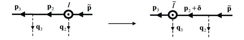
Figure 4: Example of Move left update.

Move. We can move both $\mathcal{I}$ and $\mathcal{M}$ along the lines through the whole diagram. Moving a worm along a line is only allowed if there is no other worm on this line. [Otherwise, the update is equivalent to Delete.] For example, to move $\mathcal{I}$ left (Fig. 4) we must add $\vec{\delta}$ to the line on the left from $\mathcal{I}$. This will restore the momentum conservation in $\mathcal{I}$ and create a momentum discrepancy $\vec{\delta}$ in the vertex left from $\mathcal{I}$. This is our new $\mathcal{I}$, temporarily denoted as $\tilde{\mathcal{I}}$, to avoid confusion with the old one.

The acceptance ratio of this move is given by

$$P_{\rm move}\,=\,G^{(0)}(\mathbf{p}_{2}+\vec{\delta},\tau)/G^{(0)}(\mathbf{p}_{2},\tau)\;,$$ (11)

with $G^{(0)}(\mathbf{p}_{2},\tau)$ the outgoing propagator of $\mathcal{I}$ before the update. Moving $\mathcal{I}$ to the left or right is chosen with equal probability.

Graphically, we can picture the worms as vertices with conserving momentum, provided we draw an artificial thread directly connecting the worms and transporting the momentum $\vec{\delta}$ from $\mathcal{I}$ to $\mathcal{M}$ (see Fig. 2). In this language, removing the worms means merging the thread with some path formed by the lines connecting the worms and adding the thread momentum to their momenta. If only a part of the connecting path is merged with the thread, this results in moving the worms. This way of thinking visually tells us whether we have to add or subtract $\vec{\delta}$ on lines while moving the worms.

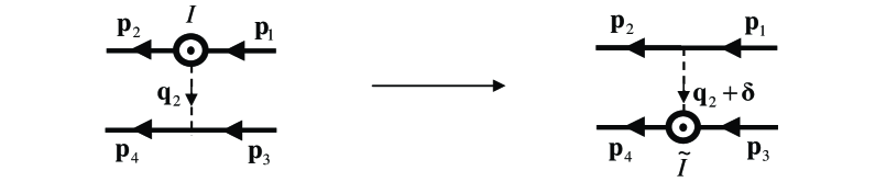
Figure 5: Example of Move down update.

Moving $\mathcal{I},\mathcal{M}$ “up” or “down” along an interaction line, we switch to a different spin component. For example, to move $\mathcal{I}$ down (up) (see Fig. 5), we have to add $\vec{\delta}$ ($-\vec{\delta}$) to the dashed line (interaction) momentum. The acceptance ratio for moving $\mathcal{I}$ down is given by

$$P_{\rm move}\,=\,U(\mathbf{q}_{2}+\vec{\delta})/U(\mathbf{q}_{2})\;.$$ (12)

Obviously, the move right/left/up/down updates are the same for $\mathcal{M}$ with the only difference that instead of adding $\pm\vec{\delta}$ to the lines we have to subtract it.

Reconnect. This simple update can be performed—and is automatically rejected otherwise—only if $\mathcal{I}$ and $\mathcal{M}$ occupy the same spin component. One swaps the incoming end of $\mathcal{I}$ with that of $\mathcal{M}$. It is important, however, that the update changes the excess momentum $\vec{\delta}$ associated with the worms. [It is also worth noting that without invoking the worms such an update would be generally impossible by momentum conservation.] If before the update the momenta on the incoming ends of $\mathcal{I}$ and $\mathcal{M}$ were $\mathbf{p}_{1}$ and $\mathbf{p}_{2}$ respectively, then after the update the new excess momentum is given by $\tilde{\vec{\delta}}=\vec{\delta}+\mathbf{p}_{2}-\mathbf{p}_{1}$.

The acceptance ratio for Reconnect is

$$P_{\rm rec}\,=\,\left|{G^{(0)}(\mathbf{p}_{1},\tau_{\mathcal{M}}-\tau_{1})~{}G^{(0)}(\mathbf{p}_{2},\tau_{\mathcal{I}}-\tau_{2})\over G^{(0)}(\mathbf{p}_{1},\tau_{\mathcal{I}}-\tau_{1})~{}G^{(0)}(\mathbf{p}_{2},\tau_{\mathcal{M}}-\tau_{2})}\right|\;,$$ (13)

with $\tau_{\mathcal{I}}$, $\tau_{\mathcal{M}}$ the imaginary times of the vertices at which $\mathcal{I}$ and $\mathcal{M}$ are located, respectively. The variable $\tau_{1}$ ($\tau_{2}$) gives the imaginary time of the vertex from which a propagator runs to the vertex of $\mathcal{I}$ ($\mathcal{M}$) with momentum $\mathbf{p}_{1}$ ($\mathbf{p}_{2}$), before the update.

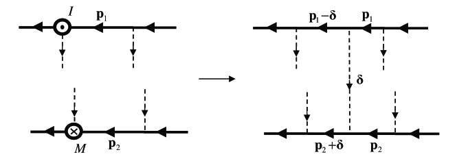
Figure 6: Add update.

Add. This update, adding a new interaction line, is only possible—being automatically rejected otherwise—if $\mathcal{I}$ and $\mathcal{M}$ have different spin components. For definiteness, we insert the new interaction line between the propagator coming into $\mathcal{I}$ and the one coming into $\mathcal{M}$, as in Fig. 6. At a randomly chosen time, these lines are broken and the four-point vertex is inserted in the breaks. In this particular realization, there is no freedom in choosing the momentum along the new dashed line: we set it equal to $\vec{\delta}$, which means that the update inevitably deletes $\mathcal{I}$ and $\mathcal{M}$.

The acceptance ratio for Add is

$$P_{\rm add} = \frac{U(\vec{\delta})}{(N+1)~{}W_{1}(\tau)~{}C_{N}}\left|\frac{G^{(0)}_{\uparrow}(\mathbf{p}_{1}-\vec{\delta},\tau_{\mathcal{I}}-\tau)~{}G^{(0)}_{\uparrow}(\mathbf{p}_{1},\tau-\tau_{1})}{G^{(0)}_{\uparrow}(\mathbf{p}_{1},\tau_{\mathcal{I}}-\tau_{1})}\right|$$ (15)

$$\times\left|\frac{G^{(0)}_{\downarrow}(\mathbf{p}_{2}+\vec{\delta},\tau_{\mathcal{M}}-\tau)~{}G^{(0)}_{\downarrow}(\mathbf{p}_{2},\tau-\tau_{2})}{G^{(0)}_{\downarrow}(\mathbf{p}_{2},\tau_{\mathcal{M}}-\tau_{2})}\right|\;,$$

where $N$ is the order of the diagram and $W_{1}(\tau)$ is the distribution from which the time $\tau$ of the new interaction vertex is drawn. We have assumed that $\mathcal{I}$ occupies the spin-up component, without loss of generality.

Remove. This update is a straightforward inverse of the previous one. It can be performed (accepted) only in the $\Sigma$-sector. It simultaneously removes an interaction line and creates a pair of worms. If the removed line had momentum $\mathbf{q}$, for $\mathcal{I}$ and $\mathcal{M}$ we shall have $\vec{\delta}=\mathbf{q}$.

In view of the indistinguishability of $\mathcal{I}$ and $\mathcal{M}$, we require that $\mathcal{I}$ ($\mathcal{M}$) is created on the spin-up (spin-down) line. The acceptance ratio of this move is given by the inverse of Eq. (15) with $N$ being the final diagram order now. Adding or removing an interaction line can also involve a change of the measuring propagator when this propagator is the incoming propagator of $\mathcal{I}$ or $\mathcal{M}$.

4 Useful Tricks and Relations

Connectivity and irreducibility. The updates discussed above are constructed in such a way that disconnected physical diagrams are never sampled. In the $\Sigma$-sector, the only update that can change the topology of the diagram is the Swap move. However, swapping the measuring propagator cannot create a disconnected piece. When we are dealing with a diagram in the $W$-sector, Add-Remove and Reconnect are the only updates that can change the topology of the diagram. These updates can create two disconnected pieces in the $W$-sector. In this case, however, each disconnected piece will contain one worm end. Going back to the $\Sigma$-sector amounts to bringing the worm ends together via Add or Reconnect, at the same time restoring the connectivity.

To keep track of the irreducibility of the diagrams, we use a hash table of lines momenta. The idea is that whenever the diagram is reducible, there is at least one propagator which carries the total momentum of the diagram. The reducibility of the diagram can then be established easily by checking the hash table and finding a momentum equal to that of the measuring propagator. We also check irreducibility right before each measurement of the self-energy.

Bold propagators. The purpose of this trick is to reduce the space of diagrams sampled by Monte Carlo. As already mentioned, this becomes essential when one is dealing with a sign-alternating series, in which the sign problem scales exponentially with the number of diagrams. Basically, the idea follows from Dyson’s equation, which allows one to reconstruct the complete function $G$ from its elementary building blocks $\Sigma$. Next, in the series for $\Sigma$, one has to eliminate all diagrams already accounted for by the replacement $G^{(0)}\to G$ done for all propagator lines. At this point the scheme becomes self-consistent. In addition, one can employ geometrical series to define screened interaction lines, and, correspondingly, eliminate all diagrams with simple fermionic loops. At the time of writing we are in the process of implementing the full version of the bold-line trick.

In the simplest implementation, we build the diagrams on a modified Green’s function $\tilde{G}$ instead of $G^{(0)}$. The function $\tilde{G}$ is obtained from $G^{(0)}$ by incorporating the lowest order “tadpole” diagram (i.e., the mean-field solution) self-consistently. This reduces the number of sampled diagrams, since all diagrams that can be split into two disconnected parts by cutting a single interaction line should be left out, being already taken into account in the new Green’s function. Mathematically, $\tilde{G}$ is obtained from Eq. (7) by simply shifting the chemical potential, $\mu_{\sigma}\longrightarrow\mu_{\sigma}-\Sigma^{(1)}_{\sigma}$, where $\Sigma^{(1)}_{\sigma}=Un_{\sigma}$ is the self-energy in the lowest order and $n_{\sigma}$ is the density of the component $\sigma$. In principle, updates creating tadpole-contributions can simply be rejected. However, to keep the Markov sampling of diagrams ergodic, the presence of a limited number of closed propagators $\tilde{G}_{\sigma}(\mathbf{k},\tau=-0)$ is allowed, but such diagrams are excluded from the statistics of $\Sigma_{\sigma}$.

Resummation of the diagrams. The use of resummation techniques is a crucial ingredient of the diagrammatic Monte Carlo approach fermipolaron . We found that the resummation methods effectively reduce the error bars, and improve convergence of the Monte Carlo results. In general, for any quantity of interest—in our case, self-energy—one constructs partial sums

$$\Sigma(N_{*})\,=\,\sum_{N=1}^{N_{*}}D_{N}F_{N}^{(N_{*})}\;,$$ (16)

defined as sums of all terms up to order $N_{*}$ with the $N$-th order terms being multiplied by the factor $F_{N}^{(N_{*})}$, which has a step-like form as a function of N: in the limit of large $N_{*}$ and $N\ll N_{*}$ the multiplication factors $F$ approach unity while for $N\to N_{*}$ they suppress higher-order contributions in such a way that the series $\sum_{N=1}^{\infty}D_{N}F_{N}^{(N_{*})}$ becomes convergent. The only other requirement is that the crossover region from unity to zero has to increase with $N_{*}$. There are infinitely many ways to construct multiplication factors satisfying these conditions. And this yields an important consistency check: final results have to be independent of the choice of $F$. In the Cesàro-Riesz summation method we have

$$F_{N}^{(N_{*})}\,=\,[(N_{*}-N+1)/N_{*}]^{\delta}\;,~{}~{}~{}~{}~{}\mbox{(Ces\`{a}ro-Riesz)}\;.$$ (17)

Here $\delta>0$ is an arbitrary parameter ($\delta=1$ corresponds to the Cesàro method). The freedom of choosing the value of Riesz’s exponent $\delta$ can be used to optimize the convergence properties of $\Sigma(N_{*})$. Empirically it was found that the factor

$$F_{N}^{(N_{*})}\,=\,C^{(N_{*})}\sum_{m=N}^{N_{*}}\exp{\left[-(N_{*}+1)^{2}/m(N_{*}-m+1)\right]}\;,$$ (18)

where $C^{(N_{*})}$ is such that $F_{1}^{(N_{*})}=1$, often leads to a faster convergence fermipolaron .

We proceed as follows. With the series truncated at order $N_{*}$, we determine the physical quantity of interest (say, number density or energy), and then extrapolate its dependence on $N_{*}$ to the $N_{*}\to\infty$ limit.

Density and energy. The density is obtained from the Green’s function through the standard relation

$$n_{\sigma}\,=\,\int_{BZ}{d\mathbf{k}\over(2\pi)^{d}}\,G_{\sigma}(\mathbf{k},\tau=-0)\;,$$ (19)

where the integration is over the first Brillouin zone. Analogously, the kinetic (hopping) energy is found as

$$E^{(\mathrm{kin})}_{\sigma}/V\,=\,\int_{BZ}{d\mathbf{k}\over(2\pi)^{d}}\,\varepsilon_{\mathbf{k}}G_{\sigma}(\mathbf{k},\tau=-0)\;,$$ (20)

and the potential (interaction) energy is obtained via

$$2E^{(\mathrm{pot})}_{\sigma}/V\,=\,{\rm lim}_{\tau^{\prime}\to\tau+0}\int_{BZ}{d\mathbf{k}\over(2\pi)^{d}}\bigg{[}-\frac{\partial}{\partial\tau}-\varepsilon_{\mathbf{k}}+\mu_{\sigma}\bigg{]}G_{\sigma}(\mathbf{k},\tau-\tau^{\prime})\;,$$ (21)

where $V$ is the volume of the system.

5 Illustrative Results

To illustrate the application of DiagMC, we simulated the equations of state—density and energy as functions of chemical potential and temperature—in one (1D) and three (3D) dimensions. Diagrammatically, there is no qualitative difference between 1D and higher-dimensional cases. Meanwhile, in 1D, where fermions are equivalent to hard-core bosons, we have the advantage of comparing DiagMC results with very accurate answers obtained with the bosonic worm algorithm Barbar_Gunes .

By the (discussed in the Introduction) Dyson argument, we expect that at any finite temperature the thermodynamic functions are analytic functions of $U$ in a certain vicinity of the point $U=0$, because this point is not singular in the case of the discrete fermionic system. Correspondingly, the expansion in powers of $U$ (that, by dimensional analysis, can be understood as the expansion in powers of the dimensionless parameter $U/T$) is supposed to be convergent at small enough $U$, or, equivalently, large enough $T$. In 1D there are no phase transitions at any finite $T$, so that one can expect that the expansion in powers of $U$ is convergent (or at least resummable) down to arbitrarily low temperatures. In higher dimensions, an essential non-analyticity of thermodynamic functions appears due to phase transitions. Hence, the simplest version of DiagMC described in this work is expected to work only at high enough temperatures.

Note that employing resummation techniques is important not only for extending the method to divergent series, or improving the series convergence properties, but also for estimating systematic errors due to extrapolation from a finite number of terms we are able to calculate.

The simulation results (plotted versus the inverse of the maximum diagram order $N_{*}$) for 1D and 3D and different resummation methods are shown in Fig. 7. In 1D the horizontal straight lines in both energy and density plots mark the exact answers obtained from simulations of two-component bosons Barbar_Gunes . The computational effort in 3D was about $4800$ CPU-hours. Note that the error bars in the final answer are dominated by the systematic $N_{*}\to\infty$ extrapolation errors which are estimated from the spread of results for different extrapolation fits and resummation methods. In particular, for density in 1D the relative uncertainty due to extrapolation is of the order of $5\%$, suggesting that going to higher $N_{*}$ is desirable, which is only possible with further implementation of the bold-line tricks.

Figure 7: The number density $n_{\sigma}$ and the total energy density $E_{\sigma}/V$ per spin component in 1D [panels (a), (b)] with $U=4.0$, $\mu_{\uparrow,\downarrow}=-0.5$, and $T=0.3$, and in 3D [panels (c), (d)] with $U=4.0$, $\mu_{\uparrow,\downarrow}=1.5$, and $T=0.5$ plotted as functions of the inverse of the maximum diagram order $N_{*}$. The exact results in 1D, $n_{\sigma}=0.2718$ and $E_{\sigma}/V=-0.3613$, were obtained from simulations of two-component bosons Barbar_Gunes . The results of different resummation procedures are shown—Cesàro sum (circles), Cesàro-Riesz with $\delta=2$ (triangles), Cesàro-Riesz with $\delta=4$ (inverted triangles), and resummation with $F^{N_{*}}_{N}$ given by Eq. (18) (diamonds), and bare series without resummation (squares). The solid lines show the best fits [linear for Cesàro, polynomial of order $\delta$ for Cesàro-Riesz, and exponential for Eq. (18)].

6 Conclusion

We have developed a diagrammatic Monte Carlo scheme for a system of interacting fermions. For illustrative results, we have obtained equations of state (density and energy as functions of chemical potential and temperature) for the repulsive Hubbard model. In its current version, the scheme applies to the range of temperatures above the critical point. Generalizations of the scheme to temperatures below the critical point are possible by using one of the following two strategies (as well as their combination). (i) A small term explicitly breaking the symmetry (relevant to the critical point) can be introduced into the Hamiltonian. The phase transition then becomes a crossover, and the convergence/resummability of series is likely to take place at any temperature. (ii) Anomalous propagators can be introduced. The latter trick naturally involves the bold-line technique which is important on its own, even above the critical point, since it reduces the number of diagrams and thus alleviates the sign problem.

Tolerance to the sign problem is the single most important feature of DiagMC. One can formulate the sign problem as the impossibility of obtaining results with small error bars for system sizes which allow a reliable and controlled extrapolation to the thermodynamic limit. Within the DiagMC approach the thermodynamic limit is obtained for free, while, as demonstrated in this work, an extrapolation to the infinite diagram order can be done sensibly before the error bars explode.

7 Acknowledgements

The work was supported by the National Science Foundation under Grant PHY-0653183, the Fund for Scientific Research - Flanders (FWO), and by the DARPA OLE program. Part of the simulations ran on the Hreidar cluster at ETH Zürich.

References

- (1) A.L. Fetter and J.D. Walecka: Quantum Theory of Many-Particle Systems (Dover, 2003)
- (2) N.V. Prokof’ev, B.V. Svistunov, and I.S. Tupitsyn: JETP 87, 310 (1998); N.V. Prokof’ev and B.V. Svistunov, Phys. Rev. Lett. 81, 2514 (1998)
- (3) M. Troyer and U.-J. Wiese, Phys. Rev. Lett. 94, 170201 (2005)
- (4) N. Prokof’ev and B. Svistunov: Phys. Rev. B 77, 020408(R) (2008); arXiv:0801.0911 (to appear in Phys. Rev. B)
- (5) T. Maier, M. Jarrell, T. Pruschke, and M.H. Hettler, Rev. Mod. Phys. 77, 1027 (2005)
- (6) N. Prokof’ev, and B. Svistunov: Phys. Rev. Lett. 99, 250201 (2007)
- (7) N. Metropolis, A.W. Rosenbluth, M.N. Rosenbluth, A.H. Teller, and E. Teller: J. Chem. Phys. 21, 1087 (1953)
- (8) W.K. Hastings: Biometrika 57, 97 (1970)
- (9) A.S. Mishchenko, N.V. Prokof’ev, A. Sakamoto, and B.V. Svistunov: Phys. Rev. B 62, 6317 (2000)
- (10) E.A. Burovski, A.S. Mishchenko, N.V. Prokof’ev, and B.V. Svistunov: Phys. Rev. Lett. 87, 186402 (2001)
- (11) E. Burovski, N. Prokof’ev, B. Svistunov, and M. Troyer: Phys. Rev. Lett. 96, 160402 (2006); New J. Phys. 8, 153 (2006)
- (12) N. V. Prokof’ev, B. V. Svistunov, and I. S. Tupitsyn: Phys. Lett. A 238, 253 (1998)
- (13) F.J. Dyson: Phys. Rev. 85, 631 (1952)
- (14) The worm code for the two-component Bose Hubbard model is the courtesy of Barbara Capogrosso-Sansone and Şebnem Güneş Söyler.