X-ray observations of parsec-scale tails behind two middle-aged pulsars

Abstract

Chandra and XMM-Newton resolved extremely long tails behind two middle-aged pulsars, J1509–5850 and J1740+1000. The tail of PSR J1509–5850 is discernible up to $5.6^{\prime}$ from the pulsar, which corresponds to the projected length $l_{\perp}=6.5d_{4}$ pc, where $d=4d_{4}$ kpc is the distance to the pulsar. The observed tail flux is $2\times 10^{-13}$ erg s^-1 cm^-2 in the 0.5–8 keV band. The tail spectrum fits an absorbed power-law (PL) model with the photon index $\Gamma=2.3\pm 0.2$, corresponding to the 0.5–8 keV luminosity of $1\times 10^{33}d_{4}^{2}$ ergs s^-1, for $n_{\rm H}=2.1\times 10^{22}$ cm^-2. The tail of PSR J1740+1000 is firmly detected up to $5^{\prime}$ ($l_{\perp}\sim 2d_{1.4}$ pc), with a flux of $6\times 10^{-14}$ ergs cm^-2 s^-1 in the 0.4–10 keV band. The PL fit to the spectrum measured from a brighter, $3^{\prime}$-long, portion of the tail yields $\Gamma=1.4$–1.5 and $n_{\rm H}\approx 1\times 10^{21}$ cm^-2; its 0.4–10 keV luminosity is $\sim 2\times 10^{31}d_{1.4}^{2}$ ergs s^-1. The luminosity of the entire tail is likely a factor of 3–4 higher. The large extent of the tails suggests that the bulk flow in the tails starts as mildly relativistic downstream of the termination shock, and then gradually decelerates. Within the observed extent of the J1509–5850 tail, the average flow speed exceeds 5,000 km s^-1, and the equipartition magnetic field is a few $\times 10^{-5}$ G. For the J1740+1000 tail, the equipartition field is a factor of a few lower. The harder spectrum of the J1740+1000 tail implies either less efficient cooling or a harder spectrum of injected electrons. For the high-latitude PSR J1740+1000, the orientation of the tail on the sky shows that the pulsar is moving toward the Galactic plane, which means that it was born from a halo-star progenitor. The comparison between the J1509 and J1740 tails and the X-ray tails of other pulsars shows that the X-ray radiation efficiency correlates poorly with the pulsar spin-down luminosity or age. The X-ray efficiencies of the ram-pressure confined pulsar wind nebulae (PWNe) are systematically higher than those of PWNe around slowly moving pulsars with similar spin-down parameters.

1. Introduction

The multiwavelength synchrotron emission from ultrarelativistic particles produced in the pulsar magnetosphere and shocked in the ambient medium is observed as a pulsar-wind nebula (PWN; Rees & Gunn 1974; Kennel & Coroniti 1994; Arons 2007; Kirk & Lyubarsky 2007). Thanks to the high sensitivity and angular resolution of the Chandra and XMM-Newton observatories, about 50 PWNe have been detected in X-rays (Kaspi et al. 2006; Gaensler & Slane 2006; Kargaltsev & Pavlov 2008, hereafter KP08). The X-ray observations have shown that PWNe have complex morphologies, including toroidal structures around the pulsar, jets along the pulsar’s spin axis, and cometary tails (see KP08 for Chandra images). In particular, if a pulsar moves with a supersonic speed, $v\gg c_{s}$, the ram pressure, $p_{\rm ram}=\rho_{\rm amb}v^{2}$, exceeds the ambient medium pressure, $p_{\rm amb}$, resulting in a bowshock PWN with a tail behind the pulsar. The well-known example of such a bowshock-tail PWN is “the Mouse PWN” produced by the young, energetic pulsar J1747$-$2958 ($\tau=26$ kyr, $\dot{E}=2.5\times 10^{36}$ ergs s^-1), which shows an X-ray tail of the projected length $l_{\perp}\sim 1$ pc (Gaensler et al. 2004). In addition to the Mouse, about a dozen X-ray PWNe with bowshock-tail morphologies have been discovered recently (KP08). Interestingly, one of the longest tails, $l_{\perp}\sim 1.5$ pc, was found behind the 3 Myr old pulsar B1929+10, with a relatively low spin-down power, $\dot{E}=3.8\times 10^{33}$ ergs s^-1 (Wang et al. 1993; Becker et al. 2006; Misanovic et al. 2007). Although most of the known PWNe are powered by much younger and more powerful pulsars, it has been noticed (Kargaltsev et al. 2007) that bowshock PWNe with extended tails are generally brighter than PWNe around slowly moving pulsars.

Table 1 Observed and derived pulsar parameters

Parameter	J1509–5850	J1740+1000
R.A. (J2000)	$15^{\rm h}09^{\rm m}27\fs 13(3)$	$17^{\rm h}40^{\rm m}25\fs 950(5)$
Decl. (J2000)	$-58^{\circ}50^{\prime}56\hbox{$.\!\!^{\prime\prime}$}1(5)$	$+10^{\circ}00^{\prime}06\hbox{$.\!\!^{\prime\prime}$}3(2)$
Epoch of position (MJD)	51,463	51,662
Galactic longitude	$319.97^{\circ}$	$34.01^{\circ}$
Galactic latitude	$-0.62^{\circ}$	$20.27^{\circ}$
Spin period, $P$ (ms)	88.9	154.1
Period derivative, $\dot{P}$ ($10^{-14}$)	0.92	2.15
Dispersion measure, DM (cm-3 pc)	137.7	23.85
Distance, $d$ (kpc)	3.8	1.4
Distance from the Galactic plane, $z$ (kpc)	0.04	0.48
Surface magnetic field, $B_{s}$ ($10^{12}$ G)	0.91	1.84
Spin-down power, $\dot{E}$ ($10^{35}$ erg s-1)	5.1	2.3
Spin-down age, $\tau=P/(2\dot{P})$, (kyr)	154	114

Note. — Based on the data from Kramer et al. (2003) and McLaughlin et al. (2002). Figures in parentheses represent $1\sigma$ uncertainties in least-significant digits quoted.

The shape of the shock, the length of the tail, and the overall appearance of the entire bowshock-tail PWN are expected to depend on the interplay between $\dot{E}$, $p_{\rm amb}$, $\rho_{\rm amb}$, and $v$, as well as on the wind magnetization parameter $\sigma$ and the angle between the pulsar’s spin axis and the direction of the pulsar’s motion. Analytical and numerical modeling of magnetized outflows in bowshock-tail PWNe has been done by Romanova et al. (2005) and Bucciantini et al. (2005; B05 hereafter), respectively. It was assumed in these works that the magnetic field in the tail is purely toroidal, and the pulsar’s velocity is aligned with the rotation axis. In addition, the numerical calculations by B05 assumed a spherically symmetric relativistic pre-shock wind with an arbitrary magnetization parameter in the framework of ideal magnetohydrodynamics (MHD), while Romanova et al. (2005) postulated an equipartition between the magnetic and particle energy densities and included magnetic field reconnection into consideration. Because of computational difficulties, the numerical calculations have been so far limited to short distances (a few shock stand-off radii) from the pulsar. To understand the large-scale properties of extended tails and facilitate their modeling (including the intrinsic anisotropy of the wind and misalignment between the pulsar velocity and spin), observations of these objects are particularly important.

Here we report on X-ray observations of very extended pulsar tails behind two middle-aged pulsars, J1509–5850 and J1740+1000. PSR J1509–5850 (hereafter J1509) was discovered in the Parkes Multibeam Pulsar Survey (Kramer et al.  2003). The pulsar is located in the Galactic plane at the dispersion measure (DM) distance of about 4 kpc (see Table 1 for the pulsar properties). To study the X-ray properties of the pulsar and look for its PWN, we observed this field with Chandra. In addition to detecting the pulsar, the observation revealed a spectacular long tail, first reported by Kargaltsev et al. (2006). It was briefly described by Hui & Becker (2007; hereafter HB07), who also reported the discovery of diffuse radio emission, possibly associated with the tail. In this paper, we provide a detailed analysis of our Chandra observation of the tail and discuss implications of our results.

Pulsar J1740+1000 (hereafter J1740) has been discovered in an Arecibo survey (McLaughlin et al. 2000), and the follow-up radio observations were carried out by McLaughlin et al. (2002). The pulsar’s properties are summarized in Table 1. At the DM distance of 1.4 kpc and Galactic latitude of $20.3^{\circ}$, J1740 belongs to a very small group of pulsars located at large distances from the Galactic plane, implying either a progenitor from the halo population or a neutron star (NS) ejected from the Galactic disk with an exceptionally high speed, $\sim 4000$ km s^-1. J1740 was observed with Chandra in 2001 (PI: Z. Arzoumanian). In a preliminary analysis of these data we detected the pulsar, but the exposure was too short to study possible extended emission and the pulsar’s spectrum. Therefore, we observed the field around J1740 in a much deeper imaging exposure with XMM-Newton. In this paper we report the discovery of the PWN associated with J1740 and focus on the analysis of the PWN properties, while the spectral and timing properties of the pulsar, including the detection of the thermal emission from the NS surface, will be presented in a separate publication (Misanovic et al., in prep.).

Our X-ray observations of the J1509 and J1740 tails and the data analysis are described in §2. We estimate the pulsar and flow velocities, the magnetic field strengths and energetics of the tails, compare these tails with the other pulsar tails currently known, and discuss the implications of our findings in §3. Our main results are summarized in §4.

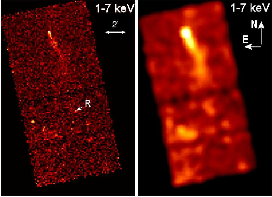
Figure 1.— Large-scale ACIS view of the J1509’s X-ray tail. The images show the S3 and S4 chips. The 1–7 keV energy band is chosen to maximize the S/N of the faint, extended tail. Both images are binned by a factor of 16 (pixel size is $7.8^{\prime\prime}$). The image on the right is additionally smoothed with the $24^{\prime\prime}$ Gaussian kernel. “R” marks the counterpart of the pointlike source projected onto the putative radio tail (see §3.2 and Fig. 14).

2. Observations and Data Analysis

J1509 was observed with the Advanced CCD Imaging Spectrometer (ACIS) on board Chandra on 2003 February 9 (ObsID 3513). The useful scientific exposure time was 39.6 ks. The observation was carried out in Very Faint mode, and the pulsar was imaged on the S3 chip, $35^{\prime\prime}$ from the optical axis (CHIPX=285, CHIPY=503). The other chips activated during this observation were S1, S2, S4, I2, and I3. The detector was operated in Full Frame mode, which provides time resolution of 3.24 s. For the analysis, we used the data reprocessed on 2006 July 20 (ASCDS ver. 7.6.8, CALDB ver. 3.2.4).

J1740 was observed with the Chandra ACIS on 2001 August 19 in Timed Exposure (imaging) mode (ObsID 1989; useful exposure time 5.1 ks) and Continuous Clocking mode (ObsID 2426; useful exposure time 16.5 ks). Only the former observation is useful for studying faint, extended features; it was carried out in Faint mode with the pulsar imaged on the S3 chip, $35^{\prime\prime}$ from the optical axis. The other activated chips were S2, I0, I1, I2, and I3, and the time resolution was 3.24 s. For the analysis, we used the data reprocessed on 2006 December 21 (ASCDS ver. 7.6.9, CALDB ver. 3.2.4).

J1740 was also observed with the European Photon Imaging Camera (EPIC) on board XMM-Newton on 2006 September 28 and 30 (observations 0403570101 and 0403570201). The EPIC PN camera was operated in Small Window mode with the reduced field-of-view (FOV) of $4^{\prime}\times 4^{\prime}$ and time-resolution of 6 ms, to analyze pulsations and perform phase-resolved spectroscopy of the pulsar. To obtain a large-scale image of the PWN, the EPIC MOS1 and MOS2 cameras were operated in Full Window Mode, which provides a larger FOV at the expense of lower time resolution (2.6 s). The Thin filter was in front of the PN and MOS cameras during both observations. The total exposures were 40.4 and 25.6 ks for the first and second observations, respectively. However, because of the reduced efficiency of the PN detector in the Small Window mode, the effective PN exposures were 28.6 ks and 17.8 ks in the first and second observations, respectively. We did not find significant flaring events in both observations (the background count rate varied by $\lesssim 20\%$). Thus, the useful scientific exposures were 66 ks for MOS1 and MOS2, and 46.4 ks for PN in the two observations combined.

The Chandra data were reduced using the Chandra Interactive Analysis of Observations (CIAO) software (ver. 3.4; CALDB ver. 3.4.0). The data obtained by XMM-Newton were reduced with the Scientific Analysis Software (SAS, ver.  7.0).

2.1. Images

The X-ray images of the J1509 and J1740 fields reveal point sources at the radio pulsar positions. The best-fit centroid positions obtained from the Chandra ACIS images, are ${\rm R.A.}=15^{\rm h}09^{\rm m}27.163^{\rm s}$, ${\rm decl.}=-58^{\circ}50^{\prime}56.12^{\prime\prime}$, and ${\rm R.A.}=17^{\rm h}40^{\rm m}25.939^{\rm s}$, ${\rm decl.}=+10^{\circ}00^{\prime}05.78^{\prime\prime}$, for J1509 and J1740, respectively. These positions differ from the corresponding radio positions by $0.3^{\prime\prime}$ and $0.6^{\prime\prime}$, respectively. The differences are comparable to the uncertainty of the absolute Chandra astrometry.

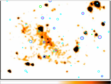
Figure 2.— Combined MOS1+MOS2 images ($18^{\prime}\times 13^{\prime}$; 0.3$-$10 keV) of the field around J1740 from two XMM-Newton observations (see text). The top panel shows a binned image (pixel size $8^{\prime\prime}$) while the bottom image (pixel size $4^{\prime\prime}$) is adaptively smoothed with a Gaussian kernel. The top panel shows the regions from which the linear brightness profiles (shown in Fig. 9) were extracted. The overlaid contours in the bottom image show optical and radio sources from the DSS2-blue (shown in cyan), DSS2-red (magenta), and NVSS 1.4 GHz (green) images.

Table 2Count statistics for PWN regions

Region	$A$	$N_{\rm tot}$	$N_{\rm bg}$	$N_{\rm src}$	S/N	$\mathcal{S}$
			J1509
Head	0.073	$118\pm 11$	$18\pm 1$	$100\pm 11$	9.1	$34.6\pm 3.8$
R1	1.16	$542\pm 23$	$249\pm 11$	$293\pm 26$	11.3	$6.38\pm 0.57$
R2	1.26	$453\pm 21$	$280\pm 12$	$173\pm 24$	7.2	$3.45\pm 0.48$
R3	2.24	$691\pm 26$	$530\pm 16$	$161\pm 31$	5.2	$1.80\pm 0.35$
Entire tail	4.68	$1686\pm 41$	$1059\pm 23$	$627\pm 47$	13.3	$3.38\pm 0.25$
			J1740
Bright portion (MOS1+2)	2.10	$1658\pm 41$	$1026\pm 32$	$632\pm 56$	11.4	$6.48\pm 0.57$
Bright portion (PN)	2.10	$2445\pm 49$	$1791\pm 42$	$654\pm 70$	9.2	$6.70\pm 0.72$

The most striking features exposed in the binned Chandra and XMM-Newton images (see Figs. 1, 2, and 3) are long linear structures (we will call them “tails” hereafter) attached to J1509 and J1740. The tails have similar orientations on the sky, with the position angles of $\approx 203^{\circ}$ for J1509, and $\approx 215^{\circ}$ for J1740 (counted east of north). Assuming that the tails are caused by the pulsar motion, the corresponding position angles of the pulsars’ proper motion can be estimated as $\approx 23^{\circ}$ and $\approx 35^{\circ}$.

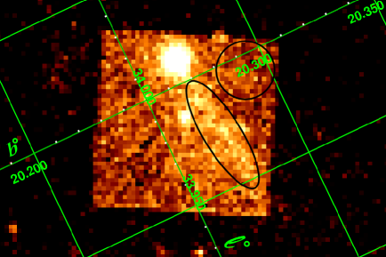
Figure 3.— $9.4^{\prime}\times 6.2^{\prime}$ binned image (pixel size $8^{\prime\prime}$) of the field around J1740 combining MOS1+MOS2 (Full Frame mode) and PN (Small Window mode) data of two XMM-Newton observations, in the 0.3$-$10 keV band (see text). The regions used for spectral extraction are marked by an ellipse (the source region) and a circle (the background). Galactic coordinate grid is shown.

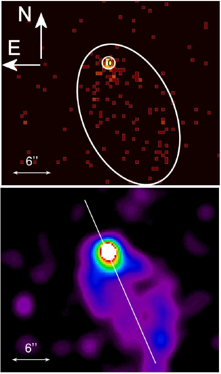
Figure 4.— Top: ACIS-S3 image of J1509 and its vicinity (1–7 keV; pixel size $0\hbox{$.\!\!^{\prime\prime}$}49$). Also shown are the extraction regions used to measure the pulsar spectrum ($r=0.9^{\prime\prime}$ circle) and the spectrum of the PWN head ($14^{\prime\prime}\times 24^{\prime\prime}$ ellipse). The radio pulsar position is shown by the small black ellipse, whose size shows the position uncertainty. Bottom: Adaptively smoothed sub-pixel resolution image (pixel size $0.25^{\prime\prime}$) of the same region obtained by removing the pipeline pixel randomization and subsequently applying the sub-pixel resolution tool (based on analyzing the charge distribution produced by an X-ray event; Tsunemi et al. 2001; Mori et al. 2001). The line shows the approximate symmetry axis of the PWN, which can be crudely identified with the direction of pulsar’s proper motion.

2.1.1 J1509 tail

The ACIS image of J1509 reveals the compact PWN ($\approx 10^{\prime\prime}\times 30^{\prime\prime}$) in the vicinity of the pulsar (see Fig. 4). Because of its elongated, elliptical shape, we will call it the “head” hereafter. Being the brightest close to the pulsar, the diffuse emission gradually broadens and becomes fainter with increasing distance from the pulsar, forming an extended tail. The tail emission is firmly detected up to $\approx 5.6^{\prime}$ (or $l_{\perp}\approx 6.5d_{4}$ pc, where $d_{4}=d/4\,{\rm kpc}$) (see Fig. 1) and possibly even farther, at a lower significance. This is demonstrated by the linear surface brightness profiles extracted along and across the tail (see Figs. 5 and 6). Although the collected number of counts from the tail is not very large (see Table LABEL:counts), the low ACIS background still allows us to detect interesting morphological changes along the tail. For instance, beyond $\sim 15^{\prime\prime}$ from the pulsar, the distribution of counts in the tail becomes asymmetric with respect to the inferred pulsar proper motion direction, shown by the dashed straight line in Figure 7 (e.g., there are more counts southeast of the line than northwest of the line). Being $\sim 40^{\prime\prime}$ wide at the $\approx 1.3^{\prime}$ distance from the pulsar, the tail slightly brightens and then suddenly narrows by about a factor of two (as shown by the small arrows in the top panel of Fig. 7). Interestingly, very similar behavior is observed in the “Mushroom PWN” (KP08) associated with another middle-aged pulsar, B0355+50 (see Fig. 7, bottom, and the images in McGowan et al. 2006). Local tail brightenings are also seen at larger distances from the J1509 pulsar (Figs. 5 and 6); however, the decreasing surface brightness of the tail and reduced off-axis resolution do not allow one to check whether or not these brightenings are accompanied by significant morphological changes.

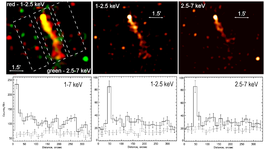
Figure 5.— ACIS images (top) of the J1509 tail (binned to the pixel size of $4^{\prime\prime}$ and smoothed with a $20^{\prime\prime}$ Gaussian kernel) in the total (1–7 keV; left), soft (1–2.5 keV; middle), and hard (2.5–7 keV; right) bands. The total band image is color coded, with the soft emission shown in red and hard emission shown in green. The bottom panels show the tail profiles in each energy band. The linear brightness profiles are obtained by extracting the source and background counts from the $1.6^{\prime}\times 6^{\prime}$ rectangular regions shown in the top left panel. The original unsmoothed images were used for the extraction. The profile extracted from the source region is plotted by the solid line while the averaged background profile extracted from the adjacent background regions is shown by the dashed line. The bin size is $15^{\prime\prime}$ in the linear profile plots.

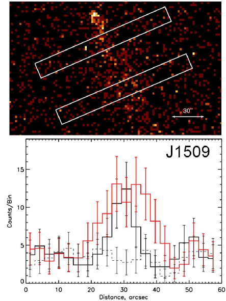
Figure 6.— Top: ACIS-S3 image (1–7 keV) showing the brightest part of the J1509 tail. Bottom: Linear profiles across the tail obtained by extracting the source counts from the two rectangular ($132^{\prime\prime}\times 15^{\prime\prime}$) regions shown in the top image. The original unsmoothed 1–7 keV image was used for the extraction. The profiles extracted from the regions closer to and farther from the pulsar are plotted by the black and red histograms, respectively. The dashed black histogram shows the averaged background profile extracted from the two background regions on both sides of the tail.

2.1.2 J1740 tail

Even in the short, 5 ks, ACIS imaging exposure of J1740 we can see traces of faint extended emission southwest of the pulsar in the heavily binned ACIS-S image (Fig. 8), and the unbinned image of the immediate vicinity of the pulsar shows an excess of counts in the same direction and perhaps some emission in front of the pulsar (see the inset in Fig. 8). The long ($\sim 5.5^{\prime}$, or $l_{\perp}\sim 2d_{1.4}$ pc, where $d_{1.4}=d/1.4\,{\rm kpc}$) tail is much better seen in the EPIC images (Figs. 2 and 3). Similar to J1509, the linear profile of the J1740 tail (see Fig. 9) hints at surface brightness fluctuations along the tail; however, detailed investigation is not possible because of the high EPIC background and poor angular resolution of XMM-Newton. In addition to the long tail, the smoothed MOS1+MOS2 image of the J1740 field (Fig. 2) and the linear profile in the east-west direction (Fig. 9) show some diffuse emission $\approx 2.5^{\prime}$ east of the pulsar, whose connection to the pulsar remains unclear. Since the XMM-Newton resolution is much more coarse than that of Chandra, emission from a number of clustered point sources may sometimes mimic the diffuse emission in the EPIC images. Therefore, we searched for point sources at radio and optical wavelengths. The bottom panel of Figure 2 shows the contours of optical and radio sources detected in the DSS2-blue, DSS2-red and NVSS (1.4 GHz) images of the region around J1740. There are a few optical sources that coincide with the X-ray pointlike sources in the EPIC images. However, the majority of optical sources in the field are faint and have no X-ray counterparts. Furthermore, the distribution of these sources shows that they cannot be responsible for the emission detected in the tail region, nor in the region $\approx 2.5^{\prime}$ east of the pulsar. Yet, until a high-resolution, deep ACIS image is obtained, we cannot exclude the possibility that some of the J1740 tail emission comes from faint point sources lacking obvious optical counterparts.

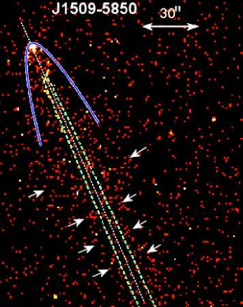
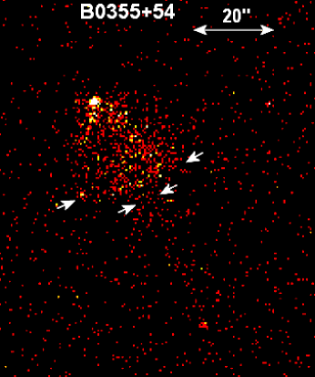
Figure 7.— Top: Images of the J1509 tail (in the 1–7 keV band, binned to the pixel size of $2^{\prime\prime}$). The parabola, $x=2.45^{\prime\prime}[(z+0.5^{\prime\prime})/1^{\prime\prime}]^{1/2}$, where $z$ is the distance from the pulsar along the tail, shows an approximate boundary of the PWN head within $\sim 15^{\prime\prime}$ from the pulsar, but it does not fit the tail’s shape at larger distances. The part of the other parabola, $x=0.44^{\prime\prime}(z/1^{\prime\prime})^{1/2}$ (shown by the dashed line), corresponds to eqs. (32–34) in Romanova et al. (2005), for $v_{mz}=10,000$ km s^-1, $v_{\rm psr}=300$ km s^-1 and $r_{0}=0.5^{\prime\prime}$ (see also §3.2). The white arrows show an approximate observed width of the tail (see text). Bottom: The Mushroom PWN powered by PSR B0355+54. Notice the sudden narrowing (transition from the “cap” to the “stem”), similar to that seen in the J1509 tail.

As the orientation of the J1740 tail on the sky indicates the proper motion direction, it provides useful information about the pulsar’s birthplace. Being located high above the Galactic plane, at $z=0.48\,d_{1.4}$ kpc, the pulsar might be a very high-speed NS if it were born in the plane (e.g., $v\gtrsim 4200\,d_{1.4}\,(114\,{\rm kyr}/t)$ km s^-1, where $t$ is the pulsar age, if it were born in the midplane of the Galaxy). However, the X-ray image of the tail, shown together with the Galactic coordinate grid in Figure 3, suggests that the pulsar is moving at a small angle, $\simeq 7^{\circ}$, toward the plane, which means that it was born well out of the Galactic plane, likely from a halo-star progenitor.

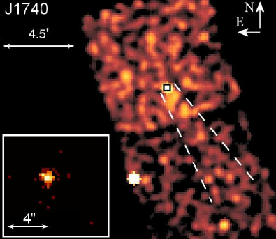
Figure 8.— ACIS images of the J1740 field. The main panel shows the binned (pixel size $7.9^{\prime\prime}$) ACIS image in the 0.5–6 keV band smoothed with a $24^{\prime\prime}$ Gaussian. Faint emission from the extended tail is visible within the region between the dashed lines. The inset shows the immediate vicinity of J1740 in the same energy band. The image resolution is maximized by applying a sub-pixel resolution tool (Tsunemi et al. 2001; Mori et al. 2001). The pixel size in the inset image is $0.25^{\prime\prime}$.

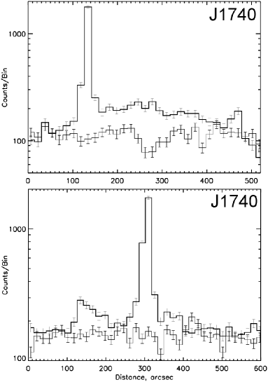
Figure 9.— Top: Linear profiles of the J1740 tail and the background obtained by extracting counts from the rectangular regions along the tail and a parallel source-free region located north-east from the tail (the two $1^{\prime}\times 11.5^{\prime}$ rectangular regions are shown in Fig. 2). Bottom: Linear profiles extracted along the east-west direction from the two $1.3^{\prime}\times 10.3^{\prime}$ rectangular regions shown in Fig. 2. The unsmoothed MOS1+MOS2 image in the 0.4–10 keV band, combining the two XMM-Newton observations, was used for the extraction.

2.2. PWN spectra

2.2.1 J1509

We extracted the spectrum of the J1509 PWN from the three numbered rectangular regions shown in Figure 10. Region 1 (R1 hereafter) includes the PWN head, but not the pulsar (we excluded counts from the $0.9^{\prime\prime}$ radius circle shown in Fig. 4). We also extracted the spectrum from the combined region 1+2+3 (although it includes the PWN head, the head contribution is small compared to that of the tail, so that we will refer to it as the “entire tail” region). For each of the regions, the background was extracted from the two corresponding rectangular regions located on both sides of the source region (see Fig. 10). The measured source and background count numbers and areas are given in Table LABEL:counts. The observed flux in the entire tail is $F_{\rm tail}=(2.0\pm 0.2)\times 10^{-13}$ ergs s^-1 cm^-2 in the 0.5–8 keV band. In addition, we extracted the head spectrum from the elliptical region shown in Figure 4 (middle panel), with the absorbed flux $F_{\rm head}=(4.9\pm 0.5)\times 10^{-14}$ ergs s^-1 cm^-2 in the 0.5–8 keV band.

Table 3PL fits to the J1509 and J1740 PWN spectra

Model	$n_{\rm H,22}$	$\mathcal{N}_{-5}$	$\Gamma$	$\chi^{2}$/dof	$L_{\rm X,32}$	$I_{-17}$	$\mathcal{B}_{-8}$
			J1509
Head	$[1.3]$	$0.7\pm 0.2$	$1.27\pm 0.25$	$7.56/9$	$1.15\pm 0.32$	23	2.7
Head	$[2.1]$	$1.4^{-0.17}_{+0.19}$	$1.83\pm 0.30$	$8.37/9$	$1.33\pm 0.41$	27	5.3
R1	$[2.1]$	$5.7_{-1.0}^{+1.2}$	$2.12^{-0.22}_{+0.19}$	$3.60/8$	$4.4\pm 0.4$	5.5	1.4
R2	$[2.1]$	$4.3_{-1.2}^{+1.7}$	$2.36\pm 0.40$	$1.68/4$	$2.9\pm 0.6$	3.7	0.95
R3	$[2.1]$	$4.7\pm 1.6$	$2.37^{-0.43}_{+0.35}$	$2.16/4$	$3.2\pm 0.7$	2.0	0.58
Entire tail	$[2.1]$	$16.5\pm 2.4$	$2.36_{-0.17}^{+0.15}$	$9.1/14$	$11.2\pm 1.0$	3.5	1.0
			J1740
Bright tail	$0.05^{+0.11}_{-0.05}$	$0.73^{+0.25}_{-0.16}$	$1.37^{+0.20}_{-0.25}$	50.9/38	$0.16\pm 0.04$	0.91	0.1
Bright tail	[0.1]	$0.80\pm 0.11$	$1.48\pm 0.19$	51.5/39	$0.15\pm 0.04$	0.88	0.1

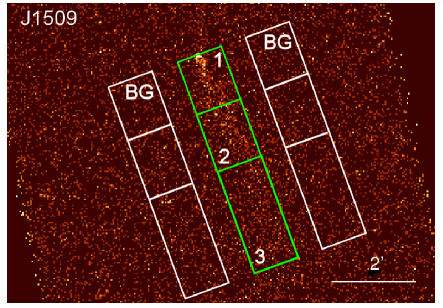
Figure 10.— Regions used to extract the spectra of the J1509 tail (see §2.2.1).

First, we fit the R1 spectrum with the absorbed power-law (PL) model, allowing the hydrogen column density, $n_{\rm H}$, to vary. The fit gives $n_{\rm H,22}\equiv n_{\rm H}/10^{22}\,{\rm cm}^{-2}=2.1_{-0.5}^{+0.7}$ (the uncertainties here and below correspond to the 68% confidence level for a single interesting parameter, i.e., $\chi^{2}-\chi_{\rm min}^{2}=1$). Fitting the same model to the R2 and R3 spectra results in larger uncertainties, while the best-fit $n_{\rm H}$ values are similar to that obtained for R1. The PL fit to the spectrum of the entire tail gives a slightly larger column density, $n_{\rm H,22}=2.5\pm 0.5$, while the fit to the head spectrum gives a somewhat lower $n_{\rm H,22}=1.3\pm 0.5$, which is still consistent with the above values (see Fig. 11). The total Galactic HI column in that direction is $n_{\rm HI,22}\approx 1.7$ (Dickey & Lockman 1990); however, this does not contradict the larger $n_{\rm H}$ values for the J1509 PWN because the $n_{\rm H}$ deduced from an X-ray spectrum under the assumption of standard element abundances generally exceeds the $n_{\rm HI}$ measured from 21 cm observations by a factor of 1.5–3 (e.g., Baumgartner & Mushotzky 2006). Finally, the value $n_{\rm H,22}=0.42$, estimated from the pulsar’s dispersion measure under the standard assumption of 10% ionization of the interstellar medium (ISM), is noticeably lower than the above values, a which possibly means that average ISM ionization is lower than 10% in the direction to J1509. Thus, given different kinds of uncertainties, we can only conclude that the true $n_{\rm H,22}$ is somewhere between 0.4 and 3. Throughout most of the analysis below we choose to fix $n_{\rm H,22}$ at the value obtained from the fit to the R1 spectrum since it has the highest S/N among the other PWN elements (see Table LABEL:counts).

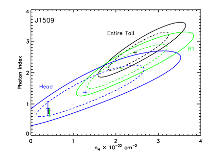
Figure 11.— Confidence contours (68% and 90%) in the $n_{\rm H}$–$\Gamma$ plane for the PL fit to the J1509 head (blue), region R1 (green), and the entire tail (black) spectra. The contours are obtained with the PL normalization fitted at each point of the grid. The $\Gamma$ values obtained from the fits with fixed $n_{\rm H,22}=0.42$ (inferred from the DM value assuming 10% ISM ionization) are shown by the error bars.

Figure 12.— Confidence contours (68% and 90%) for the PL fits to the J1509 PWN regions (labeled in the plot) for the fixed $n_{\rm H,22}=2.1$. The PL normalization is in units of $10^{-6}$ photons cm^-2 s^-1 keV^-1 at 1 keV. The dashed curves are the loci of constant unabsorbed flux in the 0.5–8 keV band; the flux values near the curves are in units of 10^-13 ergs cm^-2 s^-1.

With the fixed $n_{\rm H,22}=2.1$, the absorbed PL fits to the R1 spectrum and the entire tail spectrum result in the photon indices $\Gamma_{\rm R1}=2.1\pm 0.2$ and $\Gamma_{\rm tail}=2.4\pm 0.15$, with the unabsorbed 0.5–8 keV fluxes $F_{\rm R1}^{\rm unabs}=2.33^{+0.27}_{-0.22}\times 10^{-13}$ ergs cm^-2 s^-1 and $F_{\rm tail}^{\rm unabs}=(5.9\pm 0.5)\times 10^{-13}$ ergs cm^-2 s^-1 (see also Fig. 12 and Table 3). The unabsorbed 0.5–8 keV luminosity of the entire tail is $L_{\rm tail}\approx 1.1\times 10^{33}d_{4}^{2}$ ergs s^-1, while the luminosity of the head is a factor of 10 lower (see Table 3 for other details).

The pulsar’s spectrum will be analyzed in detail elsewhere. For the purposes of this paper, it suffices to say that the spectrum fits the absorbed PL model with $\Gamma_{\rm psr}\simeq 2.2$ and an unabsorbed 0.5–8 keV flux $F_{\rm psr}^{\rm unabs}\approx 7.8\times 10^{-14}$ ergs s^-1 cm^-2 (for $n_{\rm H,22}=2.1$), corresponding to the isotropic luminosity $L_{\rm psr}=1.5\times 10^{32}d_{4}^{2}$ ergs s^-1.

2.2.2 J1740

Since the ACIS imaging exposure of J1740 was very short, we have to rely upon the XMM-Newton data to infer the spectral properties of the extended tail. We excluded events with energies below 0.4 keV and above 10 keV from the analysis because of the large particle background contribution at these energies. We then extracted the spectrum of the bright part of the tail (within the PN FOV) from the elliptical region shown in Figure 3. The choice of the background region was limited by the size of the PN FOV in the Small Window mode, so we extracted it from the largest possible circular region, also shown in Figure 3. In the first observation we collected 1459, 471, and 492 counts (of which 25.6%, 38.0%, and 27.9% counts come from the source) in PN, MOS1, and MOS2, respectively. A slightly smaller numbers of counts were collected from the second observation: 986 (28.4% from the source) in PN, 342 (46.1%) in MOS1, and 353 (44.9%) in MOS2.

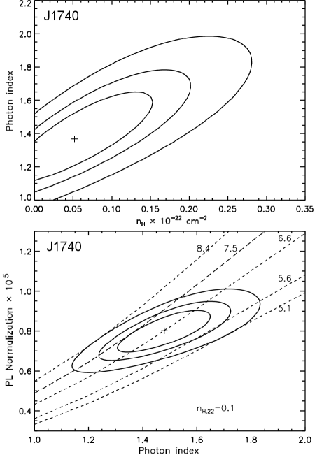
Figure 13.— Top: Confidence contours (68%, 90%, and 99%) in the $n_{\rm H}$–$\Gamma$ plane for the PL fit to the J1740 tail spectrum. The contours are obtained with the PL normalization fitted at each point of the grid. Bottom: 68%, 90%, and 99% confidence contours for the fixed $n_{\rm H}=1\times 10^{21}$ cm^-2. The dashed lines are the loci of constant unabsorbed flux in the 0.4–10 keV band; the flux values are in units of $10^{-14}$ ergs cm^-2 s^-1.

We fit the PN and MOS spectra of both observations simultaneously in the 0.4–10 keV band using an absorbed PL model. First, we fit the data with all parameters allowed to vary. The hydrogen column density obtained from this fit is poorly constrained, $n_{\rm H,22}=0$–0.16 (see Fig. 13, top, and Table 3). Then, we fixed the absorption column to the value $n_{\rm H,22}=0.1$, consistent with the pulsar’s dispersion measure assuming the 10% ISM ionization and the fits of the pulsar spectrum (Misanovic et al., in prep.). The results of the spectral fitting are shown in Table 3 and Figure 13 (bottom). The energy flux from the tail is $F_{\rm tail}=(6.0\pm 0.6)\times 10^{-14}$ ergs cm^-2 s^-1 in the 0.4–10 keV band. The tail spectrum is relatively hard, with the photon index $\Gamma_{\rm tail}=1.1$–1.7; its unabsorbed flux, $F_{\rm tail}^{\rm unabs}\approx 6.6\times 10^{-14}$ ergs s^-1 cm^-2, corresponds to the 0.4–10 keV luminosity $L_{\rm tail}\approx 1.5\times 10^{31}d_{1.4}^{2}$ ergs s^-1 ($L_{\rm tail}=1.3\times 10^{31}d_{1.4}^{2}$ ergs s^-1 in the 0.5–8 keV band).

The MOS and ACIS images (Figs. 2 and 8) suggest that the tail extends beyond the elliptical region used in the above spectral analysis, up to $\sim 7^{\prime}$ from the pulsar. However, poor statistics precludes meaningful analysis of the spectra extracted outside the PN FOV A crude estimate of the remaining tail flux can be obtained from net tail counts measured in the MOS and ACIS images outside the elliptical region. Using PIMMS and assuming $n_{\rm H,22}=0.1$ and the PL slopes inferred above, we estimated the luminosity of the entire visible tail to be $L_{\rm tail}\sim(2$–$5)\times 10^{31}d_{1.4}^{2}$ ergs s^-1.

The detailed phase-resolved analysis of the pulsar spectrum shows that it includes both thermal and non-thermal emission components (the results will be reported in a subsequent paper; Misanovic et al., in prep.). Here we just note that the non-thermal part of the spectrum fits a PL model with $\Gamma_{\rm psr}\simeq 1.2$–1.4 and luminosity $L_{\rm psr}\sim 3\times 10^{30}d_{1.4}^{2}$ ergs s^-1 in the 0.5–8 keV band.

3. Discussion

The very long tails of the J1509 and J1740 pulsars are extreme examples of ram-pressure confined outflows from supersonically moving pulsars. To date, about 13 extended X-ray sources likely associated with fast-moving pulsars have been found, although in some cases the interpretation of the observed elongated structures as tails is tentative (see KP08 for a review). The sample of well-established X-ray PWNe with long ram-pressure confined tails is still very limited (see § 3.3 and Table 5). We expanded the sample by adding the two pulsars, J1740 and J1509, with remarkably long, prominent X-ray tails.

Despite the similarities in their appearance, pulsar tails show significant differences in their X-ray spectra, luminosities, apparent lengths, surface brightness distributions, and multiwavelength properties. Below we derive physical properties of the J1509 and J1740 tails, compare them with model predictions, and discuss the physical processes that determine the tails’ appearance and spectra. We also provide a comparison with other pulsar tails, stressing the differences and discussing their possible origin.

3.1. Morphology of the tails and pulsar speeds.

The appearance of the X-ray PWNe around J1509 and J1740 clearly shows that the pulsars move with supersonic speeds. If the pulsar speed is supersonic, the shocked pulsar wind (PW) ahead of the pulsar is confined between the bow-shaped termination shock (TS) and the contact discontinuity (CD) surface, while the shocked ambient matter is confined between the CD surface and the forward shock (FS). The PWN behind the pulsar acquires an elongated shape stretched in the direction opposite to the direction of the pulsar’s motion. Recent numerical simulations by B05 show that for the idealized case of an isotropic PW the TS acquires a bullet-like shape, with the TS apex (bullet head) at the distance

$$R_{h}\approx\left[\frac{\dot{E}}{4\pi c\,(p_{\rm amb}+p_{\rm ram})}\right]^{1/2}$$ (1)

from the pulsar, where the PW pressure, $p_{w}\approx\dot{E}(4\pi cr^{2})^{-1}$, is balanced by the sum of the ambient pressure, $p_{\rm amb}$, and the ram pressure, $p_{\rm ram}=\rho v^{2}=1.67\times 10^{-10}nv_{7}^{2}$ dyn cm^-2 (here $v_{7}=v/10^{7}\,{\rm cm\,s}^{-1}$ is the pulsar speed, and $n\equiv\rho/m_{\rm H}$ is in units of cm^-3). Assuming $p_{\rm ram}\gg p_{\rm amb}$ [equivalent to ${\mathcal{M}}\gg 1$, where ${\mathcal{M}}=v/c_{s}=(3p_{\rm ram}/5p_{\rm amb})^{1/2}$ is the Mach number] we obtain

$$R_{h}\approx 4.0\times 10^{16}\,\dot{E}_{35}^{1/2}n^{-1/2}v_{7}^{-1}\,\,{\rm cm},$$ (2)

or, equivalently, $p_{\rm ram}\approx 2.65\times 10^{-9}\dot{E}_{35}R_{h,16}^{-2}$ dyn cm^-2, where $\dot{E}_{35}=\dot{E}/(10^{35}\,{\rm ergs\,s}^{-1})$, $R_{h,16}=R_{h}/10^{16}\,{\rm cm}$.

For large Mach numbers and small values of the magnetization parameter $\sigma$ of the pre-shock pulsar wind, the TS bullet’s cylindrical radius is $r_{\rm TS}\sim R_{h}$ , and the distance of its back surface from the pulsar is $R_{b}\sim 6R_{h}$ (B05). The numerical simulations (B05) and analytical models (Romanova et al. 2005) also show that an extended tail forms behind the back surface of the bullet. According to B05, the flow speed within this tail ranges from (0.8$-$0.9)$c$ in its sheath to (0.1$-$0.3)$c$ in the narrow inner channel of the tail.

For J1509, the $~{}3^{\prime\prime}$-long region of enhanced surface brightness immediately behind the pulsar (see Fig. 4, top) can be interpreted as emission from the TS bullet, implying the distance $R_{h}\sim R_{b}/6\sim 3\times 10^{16}\,(d_{4}/\sin i)$ cm to the (unresolved) TS apex ($i$ is the angle between the pulsar velocity and the line of sight). This assumption and equation (2) give $p_{\rm ram}\approx 1.5\times 10^{-9}(d_{4}/\sin i)^{-2}$ dyn cm^-2 and an estimate for the pulsar speed as a function of ambient number density,

$$v\approx 400\,\dot{E}_{35}^{1/2}n^{-1/2}R_{h,16}^{-1}\,\,{\rm km\,\,s}^{-1}\sim 300\,n^{-1/2}(d_{4}/\sin i)^{-1}\,\,{\rm km\,\,s}^{-1}.$$ (3)

Alternatively, we can estimate the Mach number as a function of ambient pressure,

$$\mathcal{M}\approx(3\dot{E}/20\pi R_{h}^{2}cp_{\rm amb})^{1/2}\sim 30\,(d_{4}/\sin i)^{-1}p_{\rm amb,-12}^{-1/2},$$ (4)

where $p_{\rm amb,-12}=p_{\rm amb}/10^{-12}\,{\rm dyn\,cm}^{-2}$ ($p_{\rm amb,-12}\sim 1$ is a typical ISM pressure in the Galactic plane; e.g., Ferrière 2001).

Unfortunately, the poor angular resolution of XMM-Newton and the shortness of the Chandra exposure do not allow us to constrain the size of the TS bullet around J1740. However, the Chandra image of the vicinity of J1740 (see the inset in Fig. 8) shows a brightening $\simeq 0.7^{\prime\prime}$ ahead of the moving pulsar. One can speculate that the brightening corresponds to the TS apex, which gives $R_{h}\sim 1.5\times 10^{16}(d_{1.4}/\sin i)$ cm. This corresponds to the pulsar speed

$$v\sim 400\,n^{-1/2}(d_{1.4}/\sin i)^{-1}\,\,{\rm km\,\,s}^{-1}$$ (5)

and the Mach number

$$\mathcal{M}\sim 130(d_{1.4}/\sin i)^{-1}p_{\rm amb,-13}^{-1/2}$$ (6)

(notice that we changed the scaling here to account for the lower pressure at large distances from the Galactic plane). The estimated pulsar speed is consistent with $v_{\perp}\sim 200$ km s^-1, inferred from the interstellar scintillation measurements by McLaughlin et al. (2002), if $n\sim 4d_{1.4}^{-2}(\sin i)^{4}$ cm^-3. It can be reconciled with the space-averaged density $n\sim 0.04$–0.05 cm^-3, expected at $z\sim 400$–500 pc (Fig. 2 in Ferrière 2001), if $\sin i\sim 0.3d_{1.4}^{1/2}$, which would correspond to $v\sim 600d_{1.4}^{-1/2}$ km s^-1, $\mathcal{M}\sim 40p_{\rm amb,-13}^{-1/2}d_{1.4}^{-1/2}$, and the tail’s length $l\gtrsim 6d_{1.4}^{1/2}$ pc.

As the ISM pressure is much more uniform than the density, the Mach number values (eqs. [4] and [6]) are more certain than the speed values in equations (3) and (5). On the other hand, the ambient pressure in the pulsar vicinity may be higher than the typical ISM pressure because the pulsar’s UV emission heats and ionizes the surrounding medium (e.g., Bucciantini & Bandiera 2001) . Therefore, the Mach numbers can be somewhat lower than the numerical values in equations (4) and (6). Also, we should not forget that our estimates are based on the assumption of isotropic distribution of the unshocked pulsar wind. The estimates may change considerably if the wind is essentially anisotropic, but no models have been published for this case so far.

3.2. Magnetic field and flow speed

Assuming some value for the ratio $k_{m}=w_{\rm mag}/w_{\rm rel}$ of the magnetic energy density, $w_{\rm mag}=B^{2}/(8\pi)$, to the energy density of relativistic particles, $w_{\rm rel}$, the magnetic field in the tails can be estimated from the measured synchrotron surface brightness (Pavlov et al. 2003):

$$B=7.2\,\left\{\frac{k_{m}}{a_{p}(3-2\Gamma)}\left[E_{{\rm M},p}^{(3-2\Gamma)/2}-E_{{\rm m},p}^{(3-2\Gamma)/2}\right]\frac{\mathcal{B}_{-8}}{\bar{s}_{17}}\right\}^{2/7}\,\,\mu{\rm G}\,.$$ (7)

Here $\mathcal{B}=\mathcal{N}/A=10^{-8}\mathcal{B}_{-8}$ photons (s cm² keV arcsec²)^-1 is the average spectral surface brightness at $E=1$ keV (see Table 3), $\mathcal{N}$ is the normalization of photon spectral flux measured in area $A$, $\bar{s}=10^{17}\,\bar{s}_{17}$ cm is the average length of the radiating region along the line of sight, $E_{{\rm m},p}=E_{\rm m}/y_{{\rm m},p}$, $E_{{\rm M},p}=E_{\rm M}/y_{{\rm M},p}$, $E_{\rm m}$ and $E_{\rm M}$ are the lower and upper energies of the photon power-law spectrum (in keV), and $y_{{\rm m},p}$, $y_{{\rm M},p}$ and $a_{p}$ are the numerical coefficients whose values depend on the slope $p=2\Gamma-1$ of the electron power-law spectral energy distribution (see Table 4 and Ginzburg & Syrovatskii 1965).

Table 4Synchrotron parameters and equipartition field

Region	$\Gamma$	$p$	$y_{{\rm m},p}$	$y_{{\rm M},p}$	$a_{p}$	$s_{\rm 17}$	$\mathcal{B}_{-8}$	$B_{\rm eq,-6}$
				J1509
Head	1.8	2.6	2.3	0.11	0.082	5	5.3	22
R1	2.1	3.2	2.9	0.22	0.072	7	1.4	16
R2	2.4	3.8	3.3	0.33	0.071	20	1.0	14
R3	2.4	3.8	3.3	0.33	0.071	20	0.6	12
				J1740
Bright portion	1.4	1.8	1.6	0.023	0.114	10	0.1	5.4

The quantities $\mathcal{B}$ and $\Gamma$ have been directly measured (Table 3), and $\bar{s}$ can be estimated assuming that it is close to the observed tail’s width. In addition to these parameters, the strength of the magnetic field depends on the boundary energies of the photon power-law spectrum, which are rather uncertain because of the lack of sensitive high-resolution observations outside the X-ray range. However, the observed softening of the J1509 tail spectrum with increasing distance from the pulsar (Table 3), as well as the decrease of the tail’s length at higher photon energies (Fig. 5), suggest that, at least for the J1509 tail, $E_{M}$ is close to the upper energy of the ACIS band, $\sim 10$ keV. The lower energy of the synchrotron spectrum is not constrained; we can only be sure that $E_{m}$ is smaller than the lower energy of the ACIS band, $\sim 0.3$ keV. In the numerical estimates (Table 4), we will assume $E_{m}=0.1$ keV and $E_{M}=10$ keV.

Under these assumptions, we obtain the equipartition magnetic fields $B_{\rm eq}\equiv Bk_{m}^{-2/7}\sim 10$–20 $\mu$G in several regions of the J1509 tail, with a hint of a decrease of $B_{\rm eq}$ with increasing distance from the pulsar (see Table 4). For the bright portion of J1740 tail, where the spectrum was measured, we found $B_{\rm eq}\sim 5$ $\mu$G.

We stress that the magnetic fields in Table 4 may differ by a factor of a few from the actual magnetic fields. First of all, if the energy range of the power-law spectrum is much broader than the 0.1–10 keV band, the magnetic field is larger than the estimates in Table 4. For instance, as $\Gamma>1.5$ ($p>2$) for the spectra of the J1509 tail, the derived magnetic field is sensitive to the unknown $E_{m}$ value: $B\propto E_{m}^{-(2\Gamma-3)/7}$. If the radio emission in the SUMSS image reported by HB07 (see also Fig. 14) indeed belongs to the J1509 tail, then the X-ray power-law spectrum might be extrapolated down to $E_{m}\sim 10^{-4}$–$10^{-2}$ keV (depending on the $\Gamma$ value), which would correspond to a factor of 1.5–6 higher magnetic fields. On the other hand, the magnetic field strength may be lower than $B_{\rm eq}$ if $k_{m}<1$ (e.g., by a factor of 1.9 if $k_{m}=0.1$.) Overall, it seems reasonable to conclude that the magnetic fields in the J1509 tail are in the range $\sim 10$–100 $\mu$G (probably closer to the upper end of this range), while the magnetic field in the J1740 tail is a factor of a few lower. To obtain more certain estimates, deeper ACIS observations and observations outside the X-ray range would be most important.

Using the magnetic field estimates, we can constrain the maximum electron Lorentz factor required for producing the observed X-ray power-law spectrum:
$\gamma_{M}\approx 7.6\times 10^{7}(E_{\rm M}/y_{{\rm M},p})^{1/2}(B/10\,\mu{\rm G})^{-1/2}\gtrsim 3\times 10^{8}$ (i.e., the maximum electron energy $E_{e,{\rm M}}\gtrsim 150$ TeV), for the J1509 tail. The Larmor radius for such electrons, $r_{L}=1.7\times 10^{8}\gamma(B/10\,\mu{\rm G})^{-1}\,\,{\rm cm}$, is $\gtrsim 4\times 10^{16}$ cm; it is smaller than the observed tail width as long as $\gamma_{M}\lesssim 10^{10}$.

The magnetic fields derived above and the measured projected tail length allow one to constrain the average projected flow speed in the tail:

$$v_{\rm flow,\perp}\sim l_{\perp}/\tau_{\rm syn}\sim 860\,(l_{\perp}/1\,{\rm pc})(B/10\,\mu{\rm G})^{3/2}(E/1\,{\rm keV})^{1/2}\,\,{\rm km}\,\,{\rm s}^{-1},$$ (8)

where

$$\tau_{\rm syn}=5.1\times 10^{8}\gamma^{-1}B^{-2}\,\,{\rm s}\sim 1100(B/10\,\mu{\rm G})^{-3/2}(E/1\,{\rm keV})^{-1/2}\,\,{\rm yr}$$ (9)

is the synchrotron cooling time [here we used the characteristic Lorentz factor, $\gamma\sim 1.4\times 10^{8}(B/10\,\mu{\rm G})^{-1/2}(E/1\,{\rm keV})^{1/2}$ for the electrons that give the main contribution to the synchrotron radiation at energy $E$]. Using equation (8), the magnetic fields in Table 4, and the highest energies at which the different regions of the J1509 tail are seen, we obtain $v_{\rm flow,\perp}\gtrsim 7,500$ km s^-1 for region R1, and $v_{\rm flow,\perp}\sim 13,000$ and 12,000 km s^-1 for regions R1+R2 and R1+R2+R3, respectively, for $d=4$ kpc. Given the uncertainty of the magnetic field estimates, the actual average flow speeds can be in the range $v_{\rm flow,\perp}\sim 5,000$–100,000 km s^-1, with higher values more plausible than lower ones. A similar consideration for the J1740 tail yields $v_{\rm flow,\perp}>1000$ km s^-1, but we should note that this is only a conservative lower limit (because the actual projected tail length is likely larger than observed), and $v_{\rm flow}=v_{\rm flow,\perp}/\sin i$ can substantially exceed the projected velocity for small $\sin i$. More certain estimates for $v_{\rm flow}$ could be obtained by direct measurements of the proper motion of the emission “clumps” (local brightenings) in the J1509 tail (see Fig. 5, bottom left), similar to the proper motion measurements of moving “blobs” in the Vela pulsar jet (Pavlov et al. 2003), which would require a series of deep ACIS observations.

Even with account for the large uncertainty, we can conclude that, at least for the J1509 tail, the flow speed is much larger than any reasonable pulsar speed. This means that the equation $\tau_{\rm syn}=l/v_{\rm psr}$, used in many papers on bowshock-tail PWNe, is inapplicable. (This equation implies that the downstream flow instantly acquires the velocity of the ambient medium [i.e., $v_{\rm flow}=v_{\rm psr}$ in the pulsar reference frame], leaving a synchrotron-emitting “trail” behind the moving pulsar.) On the other hand, the inferred flow speed is smaller than $v_{\rm flow}\sim 0.8c$–$0.9c$ obtained in numerical simulations by B05 for the bulk of the tail volume behind the TS bullet. However, those simulation were done only for the beginning of the tail (e.g., for distances $\lesssim 13R_{h}$ from the pulsar in B05), whereas we analyze a much larger extent of the tail (up to $l_{\perp}\sim 600R_{h}$). It seems plausible that the flow is mildly relativistic in the immediate vicinity behind the TS bullet, and it decelerates at larger distances because of the expansion of the overpressurized flow, entrainment of the ISM material (e.g., caused by the shear instability at the CD surface separating the fast-moving shocked PW from the shocked ambient ISM), or internal shocks in the tail.

The broadening of the J1509 X-ray tail with increasing distance $z$ from the pulsar (Fig. 6) suggests that the cross-sectional area of the tail increases up to $z\approx 1.5^{\prime}$, as $S(z)\propto z^{\kappa}$, with $\kappa\simeq 0.7-1.5$. At larger distances, $2^{\prime}\lesssim z<\lesssim 5^{\prime}$, the tail seems to have more or less constant width, although this requires confirmation with deeper observations. The observed radial expansion of the tail at large $z$ significantly exceeds the predictions by Romanova et al. (2005; eqs. [32–34]), for plausible values of $v_{\rm flow}$ and $v_{\rm psr}$ (see Fig. 7). Including the interaction between the shocked pulsar wind and shocked ambient gas at the CD surface might help to bring the model predictions in agreement with the observations. Polarimetric observations in the radio would allow one to measure the direction of the magnetic field in the tail and test whether it is consistent with the toroidal field assumption adopted in the current models. We should note that the relationship between $B$, $S$, and $v_{\rm flow}$ at given $z$ depends on the magnetic field topology. For instance, in ideal MHD models, $B\propto v_{\rm flow}^{-1}S^{-1/2}$ for purely toroidal magnetic field (B05), while $B\propto S^{-1}$ if the magnetic field is parallel to the tail direction. Deep X-ray observations would allow one to measure both $S(z)$ and $B(z)$ and test the validity of the ideal MHD approximation and the impact of the ambient matter entrainment.

3.3. Multiwavelength Aspects

The good alignment between the X-ray tail of J1509 and the elongated radio feature seen in the SUMSS image (Fig. 14) suggests their physical association (HB07). As it was noted by HB07, the larger length of the J1509 radio tail could be explained by slower synchrotron cooling of the radio-emitting electrons. However, the elongated radio feature has highly non-uniform surface brightness, with two maxima. The maximum located at $\approx 8^{\prime}$ from the pulsar is clearly associated with an unrelated point source, possibly an AGN. (The source is also seen in X-rays; it is marked “R” in Fig. 1.) The origin of the other maximum (located about $5^{\prime}$ from the pulsar) is unclear. It appears to be extended and could be a remote SNR (as suggested by Whiteoak & Green 1996), a radio galaxy, or an inhomogeneity in the pulsar wind flow (e.g., due to an internal shock or instability). To discriminate between these possibilities, deeper radio and X-ray observations are needed.

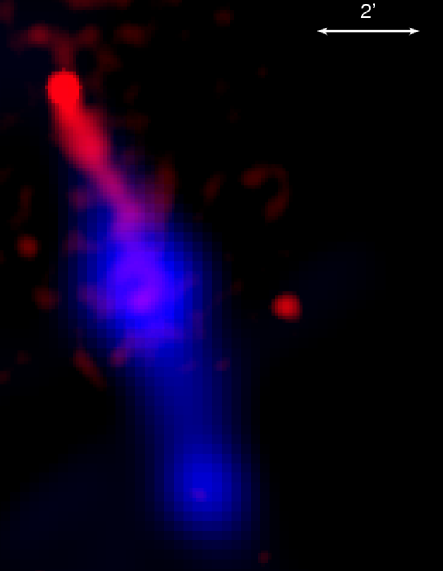
Figure 14.— Composite X-ray (red) and radio (blue) image of the field of the J1509 tail.

Another puzzling aspect is the gradual decrease in the radio surface brightness of the tail toward the pulsar (the brightness drops by at least a factor of 5 from its maximum value at $\approx 5^{\prime}$ from the pulsar), in contrast with the X-ray surface brightness that increases toward the pulsar (see Fig. 14). Unfortunately, the SUMMS image is not deep enough to show whether or not the putative radio tail actually connects to the pulsar. If the radio emission is indeed associated with the J1509 tail, the decrease in the radio surface brightness toward the pulsar cannot be explained by the synchrotron cooling because the corresponding cooling time, $\tau^{\rm radio}_{\rm syn}=1.7\times 10^{7}(B/10\mu\rm{G})^{-3/2}(\nu/1{\rm GHz})^{-1/2}$ yrs, greatly exceeds the pulsar’s age. To explain the lack of radio emission closer to the pulsar, one has to assume that the number density of particles, $n(z)$, increases with the distance from the pulsar [e.g., $n(z)\propto 1/v_{\rm flow}(z)$ for a constant cross-sectional area of the tail). This increase would not result in higher X-ray surface brightness if the most energetic electrons, responsible for the X-ray emission, undergo strong synchrotron cooling, such that their emission moves out of the X-ray band by the time when the flow reaches the distance where $n(z)$ increases substantially. Similar spatial radio-X-ray anti-correlation has been reported for the PWNe around the Vela pulsar (Dodson et al. 2003; Kargaltsev & Pavlov 2004) and PSR B1706$-$44 (Romani et al. 2005), which are moving with $\mathcal{M}\lesssim 1$ . On the other hand, in the Mouse PWN (which is the only pulsar tail well studied in the radio and X-rays) both the radio and X-ray emission are brightest near the pulsar and gradually fade with increasing $z$. Note that the Mouse X-ray tail appears to be shorter ($l_{\perp}\sim 1$ pc), or at least its X-ray surface brightness drops faster with the distance from the pulsar than in the J1509 and J1740 tails, which could result from faster cooling or lower flow speed. We also note that the remarkable $12^{\prime}$-long ($l_{\perp}=17$ pc at $d=5$ kpc) radio tail in the Mouse (Yusef-Zadeh & Gaensler 2005) is a factor of $>20$ longer than its X-ray tail, yet the radio tail remains well collimated and straight along its entire visible extent. Only deep radio observations with better angular resolution will allow one to understand the nature of the radio emission coincident with the J1509 tail and thus determine its true extent. Confirming the radio counterpart of the J1509 tail and measuring the magnetic field distribution in the radio tail will significantly advance our understanding of collimated magnetized outflows from pulsars.

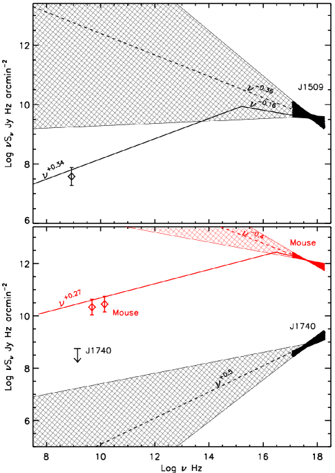
Figure 15.— Multiwavelength spectra of extended pulsar tails. For J1509 (top panel), the X-ray and radio fluxes are taken from region R2 (see Fig. 10). For J1740 (bottom panel; black), the flux is taken from the bright X-ray tail region (the ellipse in Fig. 3). For the Mouse PWN (bottom panel; red) the X-ray and radio fluxes are for the tail region as defined in the Figs. 3 and 5 of Gaensler et al. (2004). An upper limit on the J1740 1.4 GHz flux, estimated by V. Kondratiev (priv. comm.) from archival VLA data is also shown in the bottom panel. The shaded areas show the uncertainties of the X-ray spectra extrapolation. The broken solid lines show examples of possible spectra of the J1509 and Mouse tails, which are consistent with both X-ray and radio measurements (the detection of the radio tail in J1509 is tentative; see text). The spectral breaks correspond to the change of 0.5 in the spectral index due to synchrotron cooling.

The multiwavelength (radio through X-rays) spectra of the Mouse, J1509, and J1740 tails are shown in Figure 15. If the tentative interpretation of the extended radio emission as a counterpart of the J1509 X-ray tail is correct, then the tail spectrum should exhibit a spectral break between the radio and X-ray frequencies. Assuming that the break in the spatially integrated spectrum is due to the synchrotron cooling ($\Delta\Gamma\sim 0.5$), the break frequency is between $\sim 10^{12}$ and $\sim 10^{16}$ Hz, for the allowed range of the X-ray spectral slopes (an example of such a break is shown in Fig. 15 for $\Gamma_{X}=2.16$). Low-frequency breaks (in a 10–100 GHz range) have been previously reported in a number of PWNe, such as G11.2–0.3, G16.7+0.1, and G29.7–0.3 (Bock & Gaensler 2005). The spectrum of the Mouse also shows similar behavior, indicating a break around $10^{16}$ Hz (Fig. 15).

No extended radio emission has been reported around J1740. However, this could be due to the fact that the field has not yet been observed with sufficiently deep exposures. The X-ray spectrum of the J1740 tail is substantially harder than those of the J1509 and Mouse tails, suggesting a less efficient cooling or a different injection spectrum. Also, one should keep in mind that, most likely, we have detected only the $\sim 2$ pc brighter part of the J1740 tail, where the cooling makes no significant effect, while the entire tail can be substantially longer. A deep Chandra ACIS observation is necessary to reveal the true extent of the J1740 tail and search for spectral changes associated with the cooling.

So far, no TeV emission has been found in the vicinity of bowshock-tail X-ray PWNe, with the possible exception of the nebula associated with PSR B1509–58 (Aharonian et al. 2005), where the origin of the bright feature southeast of the pulsar (Gaensler et al. 2002) is not completely understood (it could be a jet, a tail, or, more likely, a combination of those, i.e., a jet behind the pulsar moving at $\mathcal{M}\sim 1$). However, the X-ray images of J1509 and J1740 reveal the presence of relativistic electrons with $\gamma\gtrsim 10^{8}$, which, for a plausible magnetic field $B\gtrsim 10$ $\mu$G, can produce TeV emission via the inverse Compton scattering of the background IR and CMB photons. Furthermore, given the large angular extent of these tails, their TeV emission can be resolved with the current TeV observatories such as HESS, MAGIC and VERITAS. The high energy GeV emission may also be detectable with GLAST if there is a substantial density of synchrotron radio photons that will be up-scattered into the GeV range.

3.4. Comparison with other pulsar tails

Table 5 summarizes the X-ray properties of eight PWNe with firmly established long X-ray tails. Two most luminous tails belong to the very young, energetic PSR J0537–6910 (located in the LMC SNR N157B) and the 26 kyr old PSR J1747–5928 (the Mouse PWN), whose X-ray efficiencies, $\eta_{\rm pwn}\equiv L_{\rm pwn}/\dot{E}$, are $2.2\times 10^{-2}$ and $1.6\times 10^{-2}$, respectively. The J1509 tail ranks third in terms of its efficiency, $\eta_{\rm pwn}\approx 2.6\times 10^{-3}$, which exceeds the efficiency of, e.g., the Duck PWN ($\eta_{\rm pwn}=3.2\times 10^{-4}$), created by the younger and more powerful PSR B1757–24, whose spin-down properties are very similar to those of PSR J1747–5928. This once again suggests that, although there is a positive correlation of $L_{\rm pwn}$ with $\dot{E}$ (see Fig. 16), the X-ray PWN luminosity also depends on other parameters (see KP08). The remaining four pulsars (B1853+01, J1740+1000, B0355+54, and B1929+10) show similar PWN efficiencies, $\eta_{\rm pwn}=(2$–$7)\times 10^{-4}$, despite the fact that their spin-down ages and powers differ by more than 2 orders of magnitude. Although some of this scatter could be attributed to the poorly known distances and different sensitivities of the individual X-ray observations, it is likely that, in addition to the spin-down parameters, there are other parameters governing the radiative efficiency of the winds in extended pulsar tails, such as the pulsar speed, the ambient pressure, and the angles between the NS magnetic and spin axes and the velocity vector.

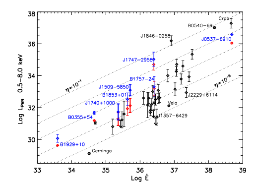
Figure 16.— X-ray luminosities of PWNe versus pulsar spin-down power (see KP08). The data points corresponding to pulsars with firmly established long X-ray tails (see Table 5) are shown in color (as well as the names of the pulsars). The blue and red points correspond to the total PWN luminosities and the luminosities of the compact bright features associated with the PWN “heads”, respectively. In most cases the luminosity of the extended tail component substantially exceeds that of the head.

In addition, for the collimated tails with nearly relativistic flow speeds, the orientation with respect to the observer can be important because the tail brightness is proportional to $(1+\beta\,\cos i)^{\Gamma+2}$, where $\beta=v_{\rm flow}/c$ and $i$ is the angle beween the velocity vector and the direction to the observer. For instance, the ratio of the brightnesses at $i=30^{\circ}$ (approaching flow) and $i=120^{\circ}$ (receding flow) can be as large as $\simeq 10$ for $\beta=0.3$ and $\Gamma=2.3$. In addition to the brightness changes, the outflow components approaching and receding at small angles will appear shorter simply as a result of projection. This might explain why the luminous X-ray tail of the more energetic Mouse PWN is so much shorter than that of the less energetic J1509, or why the X-ray tail of the Duck PWN is not only short but also very dim compared to the X-ray tail of the Mouse.

Comparing the X-ray luminosities of pulsar tails with those of PWNe around slowly moving pulsars, we see that, on average, the tails show higher X-ray efficiencies (see Fig. 16). This is a natural consequence of the fact that in the ram-pressure confined PWNe the energy of the wind flow is channeled into a narrow cylindrical structure (the tail). This results in a higher column density of emitting electrons, hence a higher surface brightness, which allows one to detect the wind emission at larger distances from the pulsar compared to PWNe around slowly moving pulsars where the wind flow is more isotropic.

If the starting flow speed just downstream of the TS back surface is more or less the same (mildly relativistic) for different pulsars, then the observed tail lengths are determined by the magnetic field strengths in the tails (because the synchrotron cooling limits the length) and by the rates at which the tail widths increase with increasing distance $z$ from the pulsar (because the tail broadening reduces its surface brightness). The magnetic field in the tail should be proportional to $(\sigma\dot{E})^{1/2}$ ($\sigma$ is magnetization parameter in the pre-shock wind). The lack of correlation with $\dot{E}$ in the current, very limited sample (Table 5) might be attributed to different wind magnetization in different pulsars and/or a large spread of the unknown inclination angles of the tails. The tail width is expected to show a negative correlation with the ambient pressure (e.g., $R_{\rm tail}\propto[\dot{E}/(v_{\rm flow}^{3}p_{\rm amb})]^{1/4}z^{1/2}$ in the Romanova et al. 2005 model); however, the dependence is too weak to be tested with the existing data.

4. Summary

We have presented a detailed analysis of the properties of two PWNe associated with the supersonically moving pulsars J1509–5850 and J1740+1000. In both cases, the X-ray images reveal parsec-scale tails connected to the pulsars. The observed extraordinary lengths of the tails suggest that the tail flow starts as mildly relativistic, and its speed remains much higher than the pulsar speed up to a distance of a few parsecs. The large extent of the J1509 tail suggests an average flow speed in excess of $\sim 5000d_{4}$ km s^-1 (a conservative lower limit). We estimate the average equipartition field in the J1509 tail to be a few $\times 10^{-5}$ G, with a hint of weakening with the distance from the pulsar. The equipartition field in the J1740 tail is likely to be a factor of a few lower. A noticeable difference between the two tails is that the spectrum of the J1740 tail is substantially harder, implying that either the cooling is not as efficient in the J1740 tail (consistent with the inferred lower magnetic field) or the electron injection spectrum of J1740 is intrinsically harder compared to that of J1509. The projected orientation of the J1740 tail on the sky suggests that the pulsar is moving toward the Galactic plane. This means that the pulsar was born well above the Galactic disk rather than ejected from the disk with a high speed.

The existing shallow radio survey data suggest a possible radio counterpart to the J1509 tail; however, a confusion with the background sources remains a possibility until better quality radio data are obtained. If the radio feature is indeed associated with the J1509 tail, then the tail spectrum should exhibit a break between 10¹² and 10¹⁶ Hz.

The comparison between the J1509 and J1740 tails and the X-ray tails from other fast-moving pulsars shows that the X-ray luminosity does not correlate well with the pulsar spindown luminosity and age; other physical parameters such as the pulsar velocity, the ambient pressure and sound speed, and the angle between the pulsar’s spin and magnetic axis may be equally important. In general, we find that the X-ray efficiencies of the ram-pressure confined PWNe are systematically higher than those of PWNe around slowly moving pulsars with similar spindown parameters.

Table 5Properties of long pulsar tails.

PSR	SNR	$d$	$v_{\perp}$	$\log\tau$	$\log\dot{E}$	$l_{\perp}$	$\log L_{\rm pwn}\tablenotemark{d}$	$\log\eta_{\rm pwn}$	Rad.	Ref.
		kpc	km s-1	[yrs]	[ergs s-1]	pc	[ergs s-1]
J0537–6910	N157B	50	600	3.70	38.68	3.7	$36.43\pm 0.02$	$-2.24$	Y	1,2
B1757–24	…	5	130	4.19	36.41	0.5	$33.20\pm 0.14$	$-3.21$	Y	3
J1747–2958	…	5	300	4.41	36.40	1.1	$34.75\pm 0.15$	$-1.65$	Y	4
J1509–5850	…	4	400	5.19	35.71	6.5	$33.04\pm 0.05$	$-2.67$	P	tw
B1853+01	W44	3	100	4.31	35.63	1.3	$32.39\pm 0.10$	$-3.24$	Y	5
J1740+1000	…	1.4	400	5.06	35.36	2	$31.54\pm 0.20$	$-3.82$	N	tw
B0355+54		$1.04^{\rm p}$	$61^{+12}_{-9}$	5.75	34.66	1.5	$31.49\pm 0.10$	$-3.16$	N	6
B1929+10	…	$0.36^{\rm p}$	$177^{+4}_{-5}$	6.49	33.59	1.5	$29.87\pm 0.25$	$-3.72$	P	7,8

References

- (1) Aharonian, F., et al. 2005, A&A, 435, L17
- (2) Arons, J. 2007, in Proc. 363rd W.E. Heraeus Seminar Neutron Stars and Pulsars , eds. W. Becker & H. H. Huang (Munich: MPE Report No. 291) (astro-ph/0708.1050)
- (3) Baumgartner, W. H., & Mushotzky, R. F. 2006, ApJ, 639, 929
- (4) Becker, W., et al. 2006, ApJ, 645, 1421
- (5) Bock, D. C.-J., & Gaensler, B. M. 2005, ApJ, 626, 343
- (6) Bucciantini, N., Amato, E., & Del Zanna, L. 2005, A&A, 434, 189 (B05)
- (7) Bucciantini, N., & Bandiera, R. 2001, A&A, 375, 1032
- (8) Chatterjee, S., Cordes, J. M., Vlemmings, W. H. T., Arzoumanian, Z., Goss, W. M., & Lazio, T. J. W. 2004, ApJ, 604, 339
- (9) Chen, Y., Wang, Q. D., Gotthelf, E. V., Jiang, B., Chu, Y-H., & Gruendl, R. 2006, ApJ, 651, 237
- (10) Cordes, J. M., & Lazio, T. J. W. 2002, preprint (arXiv:astro-ph/0207156)
- (11) Dickey, J. M., & Lockman, F. J. 1990, ARA&A, 28, 215
- (12) Dodson, R., Lewis, D., McConnell, D., & Deshpande, A. A. 2003, MNRAS, 343, 116
- (13) Ferrière, K. M. 2001, RvMP, 73, 1031
- (14) Gaensler, B. M., Arons, J., Kaspi, V. M., Pivovaroff, M. J., Kawai, N., & Tamura. K. 2002, ApJ, 569, 878
- (15) Gaensler, B. M., van der Swaluw, E., Camilo, F., Kaspi, V. M., Baganoff, F. K., Yusef-Zadeh, F., & Manchester, R. N. 2004, ApJ, 616, 383
- (16) Gaensler, B. M., & Slane, P. O. 2006, ARA&A, 44, 17
- (17) Gaensler, B. M., van der Swaluw, Camilo, F., Kaspi, V. M., Baganoff, F. K., Yusef-Zadeh, F., & Manchester, R. N. 2004, ApJ, 616, 383
- (18) Ginzburg, V. L., & Syrovatskii, S. I. 1965, ARA&A, 3, 297
- (19) Hui, C. Y., & Becker, W. 2007, A&A, 470, 965 (HB07)
- (20) Istomin, Ya. N. 2005, Astron. Rep., 49, 445
- (21) Kargaltsev, O., & Pavlov, G. G. 2004, in IAU Symp. 218, Young Neutron Stars and Their Environments, eds. F. Camilo & B. M. Gaensler (San Francisco: ASP), 195
- (22) Kargaltsev, O., Pavlov, G. G., Sanwal, D., Wong, J., & Garmire, G. P. 2006, BAAS, 38, 359
- (23) Kargaltsev, O., Pavlov, G. G., & Garmire, G. P. 2007, ApJ, 670, 643
- (24) Kargaltsev, O., & Pavlov, G. G. 2008, in 40 Years of Pulsars: Millisecond Pulsars, Magnetars, and More, eds. C. Bassa, A. Cumming, V. M. Kaspi, & Z. Wang, ASP Conf. Proc., in press (preprint arXiv0801.2602K) (KP08)
- (25) Kaspi, V. M., Gotthelf, E. V., Gaensler, B. M., & Lyutikov, M. 2001, ApJ, 562, L163
- (26) Kaspi, V. M., Roberts, M. S. E., & Harding, A. K. 2006, in Compact Stellar X-ray Sources, ed. W. H. G. Lewin & M. van der Klis (Cambridge: Cambridge Univ. Press), 279
- (27) Kennel, C. F., & Coroniti, F. V. 1984, ApJ, 283, 694
- (28) Kirk, J. G., Lyubarsky, Y., & Petri, J. 2007, in Proc. 363rd W.E. Heraeus Seminar Neutron Stars and Pulsars , eds. W. Becker & H. H. Huang (Munich: MPE Report No. 291) (astro-ph/0703116)
- (29) Kramer, M., et al. 2003, MNRAS, 342, 1299
- (30) McGowan, K. E., Vestrand, W. T., Kennea, J. A., Zane, S., Cropper, M., & Cordova, F. A. 2006, ApJ, 447, 1300
- (31) McLaughlin, M. A., Arzoumanian, Z., & Cordes, J. M. 2000, in ASP Conf. Ser. 2002, Pulsar Astronomy—2000 and Beyond, ed. M. Kramer, N. Wex, & R. Wielebinski (San Francisco: ASP), 41
- (32) McLaughlin, M. A., Arzoumanian, Z., Cordes, J. M., Backer, D. C., Lommen, A. N., Lorimer, D. R., & Zepka, A. F. 2002, ApJ, 564, 333
- (33) Misanovic, Z., Pavlov, G. G., & Garmire, G. P. 2007, ApJ, submitted (arXiv:0711.4171)
- (34) Mori, K., Tsunemi, H., Miyata, E., Baluta, C., Burrows, D. N., Garmire, G. P., & Chartas, G. 2001, in New Century of X-ray Astronomy, ASP Conf. Proc. Vol. 251. Ed. H. Inoue & H. Kunieda (San Francisco: ASP), 576
- (35) Pavlov, G. G., Teter, M. A., Kargaltsev, O., & Sanwal, D. 2003, ApJ, 591, 1157
- (36) Petre, R., Kuntz, K. D., & Shelton, R. L. 2002, ApJ, 579, 404
- (37) Rees, M. J., & Gunn, J. E. 1974, MNRAS, 167, 1
- (38) Romani, R. W., Ng, C.-Y., Dodson, R., & Brisken, W. 2005, ApJ, 631, 480
- (39) Romanova, M. M., Chulsky, G. A., & Lovelace, R. V. E. 2005, ApJ, 630, 1020
- (40) Taylor, J. H., & Cordes, J. M. 1993, ApJ, 411, 674
- (41) Tsunemi, H., Mori, K., Miyata, E., Baluta, C., Burrows, D. N., Garmire, G. P., & Chartas, G. 2001, ApJ, 554, 496
- (42) Wang, Q. D., Li, Z.-Y., & Begelman, M. C. 1993, Nature, 364, 127
- (43) Wang, Q. D., Gotthelf, E. V., Chu, Y.-H., & Dickel, J. R. 2001, ApJ, 559, 275
- (44) Whiteoak, J. B. Z. & Green, A. J. 1996, A&AS, 118, 329
- (45) Yusef-Zadeh, F., & Gaensler, B. M. 2005, AdSpR, 35, 1129