Green’s functions for solving differential equations,
in non-boundary value problems in near-field optics
and in quantum transport through point contacts

Abstract

This introduction to Green’s functions is based on their role as kernels of differential equations. The procedures to construct solutions to a differential equation with an external source or with an inhomogeneity term are put together to derive the Dyson equation for the Green’s function of the inhomogeneous system. Very different areas of physics such as, for example, electrodynamics and quantum transport, can profit from this Green’s function formalism.

The fundamental homogeneous-medium Green’s tensor of electrodynamics is deduced from the field of a dipole. Based upon that a numerical procedure is presented to solve the wave-equation for the near-field in a scattering setup for arbitrary material distributions. The full inhomogeneous system’s Green’s function is not explicitly needed to get the fields, although it can be obtained by a very similar calculation and in optics can be interpreted as a density of states.

It is demonstrated how the transport problem for two open free-electron gas reservoirs with arbitrary coupling can be solved by finding the system’s Green’s function. In this sense the article is an introduction on Green’s functions for treating interaction. A very detailed discussion of the current formula is given on an elementary basis.

I Green’s functions tool for solving differential equations

Green’s functions Ohtaka ; Don ; Koo ; Frie are encountered as response functions, time-ordered expectation values, certain solutions of boundary-value problems or resolvent kernels. This introduction to Green’s functions is based on their role as kernels of differential equations. The procedures to construct solutions to a differential equation with an external source or with an inhomogeneity term are put together to derive the Dyson equation for the Green’s function of the inhomogeneous system. Very different areas of physics such as, for example, electrodynamics (see section II and Chic ) and quantum transport (see section III and Sche98 ; Cue ), can profit from such Green’s function formalisms.

I.1 Introduction

Green’s function formalisms do not present a cure-all for solving differential equations, because essentially the problem of finding the solution of the differential equation is shifted to that of finding the corresponding Green’s function. This can, however, be a simplification and even give access to the solution of a more general class of problems. Starting from ordinary differential equations, this short review is meant to introduce how the corresponding Green’s functions are defined and how they are involved in constructing the solutions for different types of differential equations. Although bearing similarities, the Green’s function formalism can go beyond perturbation theory. Special emphasize is laid here upon the parallels between homogeneous and inhomogeneous ordinary differential and Green’s functions equations.

I.2 Homogeneous equation

The starting point is a homogeneous differential equation

$$D_{\xi}\;\phi_{0}(\xi)=0$$ (1)

which we suppose is exactly solvable, although $\phi_{0}(\xi)$ will not explicitly be needed. $D_{\xi}$ is some differential operator which may include multiplication with a constant or even another function of $\xi$. $\xi$ is either a space or time variable. What we need to know is the solution $g$ of the corresponding Green’s functions equation

$$D_{\xi}\;g(\xi,\xi^{\prime})=\delta(\xi-\xi^{\prime})$$ (2)

$g$ is a tensor-like function of two arguments, $D_{\xi}$ only acting on the first of them. Like $g$ replaces $\phi$ on the left, the zero on the right side of (1) is replaced by a $\delta$-distribution in (2). There is no general recipe, but knowing $\phi_{0}(\xi)$ can help to get $g(\xi,\xi^{\prime})$.

I.3 Source term

Having $g$, the construction of a solution

$$\phi_{q}(\xi)=\phi_{0}(\xi)+\int d\xi^{\prime}\;g(\xi,\xi^{\prime})\;Q(\xi^{\prime})$$ (3)

of the differential equation with a source term $Q$ on the right side

$$D_{\xi}\;\phi_{q}(\xi)=Q(\xi)$$ (4)

is straight forward. Of course, a solution $\phi_{0}$ of (1) can be added independently of $Q$, so we only need to proove that the integral term from (3) satisfies (4):

$$D_{\xi}\int d\xi^{\prime}\;g(\xi,\xi^{\prime})\;Q(\xi^{\prime}) = \int d\xi^{\prime}\;[D_{\xi}\;g(\xi,\xi^{\prime})]\;Q(\xi^{\prime})$$

$$= \int d\xi^{\prime}\;\delta(\xi-\xi^{\prime})\;Q(\xi^{\prime})=Q(\xi)$$

(All integrals are understood to range over the entire $\xi$-space.)

I.4 Inhomogeneity

Instead of a source term, the differential equation can contain a potential term which we shall call an inhomogeneity.

$$D_{\xi}\;\phi_{ih}(\xi)-V(\xi)\;\phi_{ih}(\xi)=0$$ (5)

that is a $\xi$-dependent function $V$ multiplied with $\phi$. $V(\xi)$ is not included in $D_{\xi}$, because we assume that it so much complicates the equation that a standard solution is no longer known. The minus sign is a useful convention. We put the inhomogeneity term on the right

$$D_{\xi}\;\phi_{ih}(\xi)=V(\xi)\;\phi_{ih}(\xi)$$ (5a)

to make (5) formally look like (4). With $V\phi$ playing the role of $Q$ a formal solution is constructed analogously to (3):

$$\phi_{ih}(\xi)=\phi_{0}(\xi)+\int d\xi^{\prime}\;g(\xi,\xi^{\prime})\;V(\xi^{\prime})\;\phi_{ih}(\xi^{\prime})$$ (6)

This presents an implicit equation for $\phi_{ih}$, the so-called Lippmann-Schwinger equation. We have replaced the differential equation by an integral equation. Inserting the solution of the homogeneous equation $\phi_{0}$ also for $\phi_{ih}$ in the integral on the right side of (6) would give the Born approximation $\phi_{ih}(\xi)\approx\phi_{0}(\xi)+\int d\xi^{\prime}\;g(\xi,\xi^{\prime})\;V(\xi^{\prime})\;\phi_{0}(\xi^{\prime})$, which is appropriate if $V\phi$ is a small perturbation compared to $D_{\xi}\phi$. However, it is the virtue of the Green’s functions method that in contrast to perturbation theory the inhomogeneity need not be a small deviation. Although not yet providing an explicit solution for $\phi_{ih}$, one can make use of (6) in numerical calculations (see section II and DerGir ). As (2) is the corresponding Green’s function equation with a point source to the homogeneous equation (1), the equation defining the Green’s function $G$ for the inhomogeneous case derived from (5) reads:

$$[D_{\xi}-V(\xi)]\;G(\xi,\xi^{\prime})=\delta(\xi-\xi^{\prime})$$ (7)

However, while supposing that we know or can easily guess $g(\xi,\xi^{\prime})$, there is no hint yet how to calculate $G(\xi,\xi^{\prime})$.

I.5 General case

Finally we have to treat the most general case with source and inhomogeneity term:

$$D_{\xi}\;\phi_{ihq}(\xi)-V(\xi)\;\phi_{ihq}(\xi)=Q(\xi)$$ (8)

In analogy to (3) and (4) a yet formal solution can be written down using (7):

$$\phi_{ihq}(\xi)=\phi_{ih}(\xi)+\int d\xi^{\prime}\;G(\xi,\xi^{\prime})\;Q(\xi^{\prime})$$ (9)

Here we have the freedom to add any solution of (6) to the integral.

But let us start again solving the problem directly from (8) which we rewrite as

$$D_{\xi}\;\phi_{ihq}(\xi)-Q(\xi)=V(\xi)\;\phi_{ihq}(\xi)$$ (8a)

We compare this with (5a) and construct a solution of the same form as (6). $\phi_{q}$ takes the role of $\phi_{0}$, because it would satisfy (8a) if the right side were zero. $\phi_{ih}$ has to be replaced by $\phi_{ihq}$. Using (3) for $\phi_{q}$ we obtain

$$\phi_{ihq}(\xi)=\underbrace{\phi_{0}(\xi)+\int d\xi^{\prime}\;g(\xi,\xi^{\prime})\;Q(\xi^{\prime})}_{\phi_{q}}+\int d\xi^{\prime\prime}\;g(\xi,\xi^{\prime\prime})\;V(\xi^{\prime\prime})\;\phi_{ihq}(\xi^{\prime\prime})$$ (10)

(10) could also have been established by a different line of thought. In (8) putting everything that differs from the homogeneous equation (1) on the right side gives

$$D_{\xi}\;\phi_{ihq}=Q(\xi)+V(\xi)\;\phi_{ihq}(\xi)$$ (8a)

If it were not for the inhomegeneity term $V\phi$, the solution would be (3). And if it were not for the source term $Q$, we could use (6). Although this is, of course, not a correct way to solve non-homogeneous differential equations, we can understand (10) as an ansatz adding these two contributions. The $\phi_{0}$-part does not have to be written twice. And $\phi_{ihq}$ has to appear instead of $\phi_{ih}$ in the integral taken from (6). This still unknown $\phi_{ihq}$ leaves the neccessary freedom to somehow counterbalance the $Q$-term not present in (5) and (6), which justifies (10) as an ansatz. Whichever way it was obtained, (10) is an implicit integral equation for $\phi_{ihq}$ as (6) is for $\phi_{ih}$.

I.6 Dyson equation

Now we shall profit from the fact that with (9) we have a second representation of $\phi_{ihq}$. Insert the expression from (9) for $\phi_{ihq}$ both on the left and on the right side in (10):

$$\phi_{ih}(\xi) + \int d\xi^{\prime}\;G(\xi,\xi^{\prime})\;Q(\xi^{\prime})=\phi_{0}(\xi)+\int d\xi^{\prime}\;g(\xi,\xi^{\prime})\;Q(\xi^{\prime})+$$

$$\int d\xi^{\prime\prime}g(\xi,\xi^{\prime\prime})\;V(\xi^{\prime\prime})\;[\;\phi_{ih}(\xi^{\prime\prime})+\int d\xi^{\prime}\;G(\xi^{\prime\prime},\xi^{\prime})\;Q(\xi^{\prime})\;]$$

$\phi_{ih}$ on the left cancels with $\phi_{0}$ and one integral term on the right according to (6) and we are left with

$$\int d\xi^{\prime}\;G(\xi,\xi^{\prime})\;Q(\xi^{\prime}) = \int d\xi^{\prime}\;g(\xi,\xi^{\prime})\;Q(\xi^{\prime})+$$

$$\int d\xi^{\prime\prime}\int d\xi^{\prime}\;g(\xi,\xi^{\prime\prime})\;V(\xi^{\prime\prime})\;G(\xi^{\prime\prime},\xi^{\prime})\;Q(\xi^{\prime})$$

This is an implicit equation for the unknown Green’s function $G$. But as $G$ by definition (7) does not depend on any source term, (11) must be valid for arbitrary $Q$. The special choice $Q(\xi^{\prime})=\delta(\xi^{\prime}-\xi_{0})$ gives

$$\int d\xi^{\prime}\;G(\xi,\xi^{\prime})\;\delta(\xi^{\prime}-\xi_{0}) = \int d\xi^{\prime}\;g(\xi,\xi^{\prime})\;\delta(\xi^{\prime}-\xi_{0})+$$

$$\int d\xi^{\prime\prime}\int d\xi^{\prime}\;g(\xi,\xi^{\prime\prime})\;V(\xi^{\prime\prime})\;G(\xi^{\prime\prime},\xi^{\prime})\;\delta(\xi^{\prime}-\xi_{0})$$

which after carrying out the $\xi^{\prime}$-integrals and then renaming $\xi_{0}$ to $\xi^{\prime}$ becomes

$$G(\xi,\xi^{\prime})=g(\xi,\xi^{\prime})+\int d\xi^{\prime}\;g(\xi,\xi^{\prime\prime})\;V(\xi^{\prime\prime})\;G(\xi^{\prime\prime},\xi^{\prime})$$ (11)

(11) is the general implicit integral equation for the inhomogeneous system’s Green’s function $G$ and called Dyson equation.

We could have derived (11) by doing all calculations from (8) on with only a point source $\delta(\xi-\xi_{0})$ instead of $Q(\xi)$. Putting in the solutions (3) and (9) for this case would just have looked a bit awkward. (11) is not an explicit solution for $G$, but still an implicit equation, and even though it is often written as $G=g+gVG$ one must not forget that there is a convolution-like integration over the inner $\xi$-index behind the sequence of factors $gVG$. The integration can either be transformed into a discrete finite sum, and thus (11) into a linear system of equations solvable by a matrix inversion (see section II and EPJ ), or the convolution can be replaced by a multiplication going to frequency space by a Fourier transformation (see section III and Cue ).

(10) and the preparation for (11) would have looked much more elegant leaving out $\phi_{0}$ and the $\phi_{ih}$-terms right from the start. Indeed, one could argue that in (3) one is only interested in the part different from the trivial homogenous solution, if no further boundary conditions have to be accounted for. With a similar argument, the $\phi_{ih}$-part could have been dropped in (9). The identities

$$\phi_{q}^{*}(\xi)=\int d\xi^{\prime}\;g(\xi,\xi^{\prime})\;Q(\xi^{\prime})$$ (3*)

$$\phi_{ih}^{*}(\xi)=\int d\xi^{\prime}\;g(\xi,\xi^{\prime})\;V(\xi^{\prime})\;\phi_{ih}^{*}(\xi^{\prime})$$ (6*)

$$\phi_{ihq}^{*}(\xi)=\int d\xi^{\prime}\;G(\xi,\xi^{\prime})\;Q(\xi^{\prime})$$ (9*)

$$\phi_{ihq}^{*}(\xi)=\int d\xi^{\prime}\;g(\xi,\xi^{\prime})\;Q(\xi^{\prime})+\int d\xi^{\prime\prime}\;g(\xi,\xi^{\prime\prime})\;V(\xi^{\prime\prime})\;\phi_{ihq}^{*}(\xi^{\prime\prime})$$ (10*)

would obviously also have given (11). Leaving out $\phi_{0}$ in (6) would be precarious (see below). However, dropping it when constructing (11) along our second line of thought causes no problem. The term with $Q$ will ensure that $\phi_{ihq}^{*}$ cannot simply be zero.

I.7 Expansions

There is some subtlety about the $\phi_{0}$ contribution in (6). (6*) has the trivial solution $\phi_{ih}^{*}(\xi)=0$ and not necessarily another one. Surely, $\phi_{ih}(\xi)=0$ satisfies (5), but it is not what we want. $\phi_{0}$ is the background excitation replacing boundary conditions in this kind of problem, which shall become clear when discussing electrodynamics (see following article). $\phi_{0}$ acts as a source term which - instead of being put in $Q$ - can be more appropriately and conveniently set as a fixed part of the $\phi$ we are looking for. Inserting (6) into itself ever and ever again, $\phi_{ih}$ is developed into a series in powers of $gV$:

$$\phi_{ih} = \phi_{0}+\int gV\phi_{ih}$$ (12)

$$= \phi_{0}+\int gV(\phi_{0}+\int gV(\phi_{0}+\int gV(\ldots\;\ldots\;\ldots)))$$

$$= \phi_{0}+gV\phi_{0}+gVgV\phi_{0}+\ldots=\sum_{n=0}^{\infty}(gV)^{n}\phi_{0}$$

Just for shorthand notation we dropped the arguments and integration variables and in the third line also the integral signs. The resulting series is recognized from perturbation theory summing interactions to zeroth, first, second, etc. order. If there were no contribution $\phi_{0}$ in $\phi_{ih}$, only the contribution of $gV$ to power infinity would exist with nothing to multiply to at the end. In other words we would have no basis on which to develop $\phi_{ih}$. The Green’s functions formalism as we use it aims at solving (6), (10) or (11) in a closed form, not cutting the series in (12) at some finite order. The development (12) is only shown here precisely to demonstrate that interactions are included to all orders as well as to explain the importance of the homogeneous background contribution. The Dyson equation (11) can be expanded in an analogous manner to the Lippmann-Schwinger equation, by the way prooving the equivalence to its complementary form $G=g+GVg$:

$$G=g+\int gVG=g\sum_{n=0}^{\infty}(Vg)^{n}=\sum_{n=0}^{\infty}(gV)^{n}\;g=g+\int GVg$$ (13)

(Integration over inner arguments is understood in all contributions to the sums.) Either formally or as a matrix calculation in finite discrete $\xi$-space, (11) is often solved as

$$G=({\bf 1}-gV)^{-1}g$$ (14)

Developing the $(\ldots)^{-1}$-factor in (14) into a geometric series just results in the infinite sums written in (13).

Putting together (12) and (13) we can get an alternative representation to (6) for the solution of the inhomogeneous differential equation:

$$\phi_{ih}(\xi)=\phi_{0}(\xi)+\int d\xi^{\prime}\;G(\xi,\xi^{\prime})\;V(\xi^{\prime})\;\phi_{0}(\xi^{\prime})$$ (15)

Therefore in the case that should it be easier to get the Green’s function $G$ than to solve the implicit equation (6) for $\phi_{ih}$, we see that $G$ can be useful also for treating the equation without an external source $Q$. Nevertheless, (15) again illustrates that $V\phi_{0}$ plays the role of the source.

I.8 Conclusions and Outlook for section I

Using Green’s functions it has been shown how differential equations can be treated that differ from easily solvable ones by an additional potential term or an arbitrary source term. The formalism as presented here is for open-boundary in contrast to boundary-value problems Koo ; Jac . From constructing the solutions of the differential equations, we also obtained the constituting relation for the inhomogeneous system’s Green’s function, which characterizes the response to a point source and includes all-order interactions. Examples of applications will be given in the two following sections.

II Non-boundary value problems in near-field optics

The fundamental homogeneous-medium Green’s tensor of electrodynamics is deduced from the field of a dipole. Based upon that a numerical procedure is presented to solve the wave-equation for the near-field in a scattering setup for arbitrary material distributions. The full inhomogeneous system’s Green’s function is not explicitly needed to get the fields, although it can be obtained by a very similar calculation and in optics can be interpreted as a density of states.

II.1 Introduction

The typical problem in nano-optics Gre97 ; DerChem is the situation that some tiny structures are illuminated by an extended source, a plane wave for example, and then one is interested in the field distribution that arises from multiple scattering scat , especially to identify places where the field intensity gets considerably enhanced Martinres ; Ebbfluo . A theory can be based on Green’s functions, however, their implication differs slightly from the standardly taught cases of fixed boundary field values Jac_1 or located sources. Modern optical scanning microscopes make it possible to probe and map directly even different quantities of the near-field interpret , such as the electric and magnetic field intensities Eloise or the density of states Chicel . Applications of tayloring nano-structures with respect to optical properties include resonant particles dicro ; partweb and cavities Krenncav ; Perney , squeezed fields squeeze , wave guides and their adressing adres ; MarLith ; Quidwave as well as transmission apertures Perney ; Thio and lithography masks MarLith . We here present the Green’s functions formalism that forms the bases of a finite-element quite effective numerical algorithm used in current research girneu ; EPJel ; coral . This treatise is also given as an application example of the general methods to solve differential equations with certain perturbations presented in the preceeding paper.

II.2 Problem

The discussion can be reduced to monochromatic light, that is a single frequency $\omega$ and thus time dependence $e^{-i\omega t}$ for the fields. With non-magnetic materials the problem is to find the solution $\vec{E}(\vec{r})$ of the wave equation

$$-\vec{\nabla}\times\vec{\nabla}\times\vec{E}(\vec{r})+\frac{\omega^{2}}{c^{2}}\;\varepsilon(\vec{r})\;\vec{E}(\vec{r})=0$$ (1)

(1) is a differential equation of the type (5) from section I. There is no source term on the right hand side of (1). If the source were, for example, a dipole located at some point, a source term with its oscillation strength and direction would have to be put on the right as $\vec{Q}\delta(\vec{r}-\vec{r}_{0})$. However, we shall see that a plane-wave source can be and is better included in (1) as it is. For simplicity we shall assume that the background medium, in which objects with different permittivities $\varepsilon$ are located (Fig.1), is vacuum with permittivity $\varepsilon_{0}$. For another embedding medium, its dielectric constant $\varepsilon_{b}$ would take the role of $\varepsilon_{0}$. In (1) $\varepsilon(\vec{r})$ of the material distribution designates the dimensionless relative permittivity with respect to vacuum or the background medium. To separate (1) into a part representing a homogeneous differential equation with known solution and an inhomogeneity write its as

$$-\vec{\nabla}\times\vec{\nabla}\times\vec{E}(\vec{r})+\frac{\omega^{2}}{c^{2}}\;\vec{E}(\vec{r})+\frac{\omega^{2}}{c^{2}}\;(\varepsilon(\vec{r})-1)\;\vec{E}(\vec{r})=0$$ (1a)

The correspondances to the quantities of the general formalism given in section I are

$$\xi\leftrightarrow\vec{r},\;D_{\xi}\ldots\leftrightarrow-\vec{\nabla}\times\vec{\nabla}\times\ldots+\frac{\omega^{2}}{c^{2}}\cdot\ldots,\;V\leftrightarrow-\frac{\omega^{2}}{c^{2}}(\varepsilon-1),\;\phi_{ih}\leftrightarrow\vec{E}$$

and $\phi_{0}$ will become $\vec{E}_{b}$. We can write down the solution following section I after having prepared the background Green’s function in the next section.

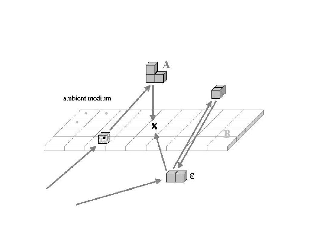
Figure 1: Objects distributed in space and discretized into cubes of equal size. A plane in space discretized into a quadratic mesh is also shown. Arrows indicate only some possible scattering paths to a location marked by the cross.

II.3 Background Green’s function

In any case we need the Green’s function $g(\vec{r},\vec{r^{\prime}})$ of the homogeneous problem satisfying

$$-\vec{\nabla}_{\vec{r}}\times\vec{\nabla}_{\vec{r}}\times g(\vec{r},\vec{r^{\prime}})+k^{2}g(\vec{r},\vec{r^{\prime}})={\bf 1}\;\delta(\vec{r}-\vec{r^{\prime}})$$ (2)

with $k=\omega/c$. $g$ will be a $3\otimes 3$ tensor or matrix here. More commonly Chew the small letter $g$ is used for the scalar function

$$g_{scal}(\vec{r},\vec{r^{\prime}})=-\frac{e^{ik|\vec{r}-\vec{r^{\prime}}|}}{4\pi|\vec{r}-\vec{r^{\prime}}|}\quad{\rm fulfilling}$$

$$\triangle_{\vec{r}}\;g_{scal}(\vec{r},\vec{r^{\prime}})+k^{2}g_{scal}(\vec{r},\vec{r^{\prime}})=\delta(\vec{r}-\vec{r^{\prime}})$$ (3)

with $k=\omega/c$. The Green’s function $g$ from (2) is then named $G^{h}$ with index $h$ for homogeneous. There are several ways to obtain $g$. One is based on the knowledge that if we have a scalar function $\Psi(\vec{r})$ solving $\triangle\Psi+k^{2}\;\Psi=0$, then $\vec{F}_{1}=\vec{\nabla}\times(\vec{a}\Psi)$ and $\vec{F}_{2}=\vec{\nabla}\times\vec{\nabla}\times(\vec{a}\Psi)$ with a constant but arbitrary pivot vector $\vec{a}$ will both solve the vectorial equation $-\vec{\nabla}\times\vec{\nabla}\times\vec{F}+k^{2}\vec{F}=0$. The tensor $g$ looked for in (2) can be constructed out of $\vec{F}_{1}(\vec{r})$, $\vec{F}_{1}(\vec{r^{\prime}})$, $\vec{F}_{2}(\vec{r})$, $\vec{F}_{2}(\vec{r^{\prime}})$ together with $\vec{F}_{3}(\vec{r})=\vec{\nabla}\Psi(\vec{r})$ and $\vec{F}_{3}(\vec{r^{\prime}})$. We shall not enter into the details of this mathematically slightly precarious approach AD . A second recipe just mentioned here for completeness is given by the following statement Chew : If $g_{scal}(\vec{r},\vec{r^{\prime}})$ satisfies (3), then

$$g(\vec{r},\vec{r^{\prime}})=({\bf 1}+\frac{\vec{\nabla}_{\vec{r}}\otimes\vec{\nabla}_{\vec{r}}}{k^{2}})\;g_{scal}(\vec{r},\vec{r^{\prime}})$$ (4)

is the tensor defined by (2). Of course, because of being in homogeneous space $g_{scal}$ and $g$ effectively are functions of $\vec{R}=\vec{r}-\vec{r^{\prime}}$ alone. ${\bf 1}$ is the unit matrix in 3 by 3 cartesian coordinate space and
$\vec{\nabla}\otimes\vec{\nabla}$ means building a matrix out of derivatives $\begin{pmatrix}\partial^{2}_{x}&\partial_{x}\partial_{y}&\partial_{x}\partial_{z}\cr\partial_{y}\partial_{x}&\partial^{2}_{y}&\partial_{y}\partial_{z}\cr\partial_{z}\partial_{x}&\partial_{z}\partial_{y}&\partial^{2}_{z}\cr\end{pmatrix}$.

We shall deduce $g$ from a physical reasoning. From standard electrodynamics Jac_2 one has the electric field of an oscillating dipole

$$\vec{E}(\vec{R})=\frac{k^{2}e^{ikR}}{4\pi\varepsilon_{0}R}\left(\frac{\vec{p}R^{2}-\vec{R}(\vec{R}\vec{p})}{R^{2}}+\frac{3\vec{R}(\vec{R}\vec{p})-\vec{p}R^{2}}{R^{2}}\left(\frac{1}{k^{2}R^{2}}-\frac{i}{kR}\right)\right)$$ (5)

It is important to take the exact formula here including retardation in contrast to common near- or far-field approximations. (5) gives the space part, the time dependence is just $e^{-i\omega t}$ everywhere. To get the Green’s tensor, we have to evaluate from (5) what field components in x-, y- and z-direction a dipole $\vec{p}$ at $\vec{r^{\prime}}$ oriented along x would produce at $\vec{r}$, what components a dipole oriented along y would produce and what components a dipole along z would produce and assemble all these in a matrix. A point dipole is the elementary excitation corresponding to the $\delta$ on the right side of (2). The physical meaning of $g$ is to tell us what field any such dipole would have. That is shown formally in the first matrix in (5a). Decomposing any $\vec{p}$ into its cartesian components, (5) can be rewritten as

$$\vec{E}(\vec{R})=\begin{pmatrix}E_{x}(\vec{r})\leftarrow p_{x}(\vec{r^{\prime}})&\phantom{e}&E_{x}(\vec{r})\leftarrow p_{y}(\vec{r^{\prime}})&\phantom{e}&E_{x}(\vec{r})\leftarrow p_{z}(\vec{r^{\prime}})\cr E_{y}(\vec{r})\leftarrow p_{x}(\vec{r^{\prime}})&\phantom{e}&E_{y}(\vec{r})\leftarrow p_{y}(\vec{r^{\prime}})&\phantom{e}&E_{y}(\vec{r})\leftarrow p_{z}(\vec{r^{\prime}})\cr E_{z}(\vec{r})\leftarrow p_{x}(\vec{r^{\prime}})&\phantom{e}&E_{z}(\vec{r})\leftarrow p_{y}(\vec{r^{\prime}})&\phantom{e}&E_{z}(\vec{r})\leftarrow p_{z}(\vec{r^{\prime}})\cr\end{pmatrix}\begin{pmatrix}p_{x}\cr p_{y}\cr p_{z}\cr\end{pmatrix}$$

${\displaystyle=\frac{k^{2}e^{ikR}}{4\pi\varepsilon_{0}R}\left(\left(1-\frac{1-ikR}{k^{2}R^{2}}\right)\begin{pmatrix}1&0&0\cr 0&1&0\cr 0&0&1\cr\end{pmatrix}\begin{pmatrix}p_{x}\cr p_{y}\cr p_{z}\cr\end{pmatrix}-\frac{-3+3ikR+k^{2}R^{2}}{k^{2}R^{4}}\begin{pmatrix}X^{2}&XY&XZ\cr YX&Y^{2}&YZ\cr ZX&ZY&Z^{2}\cr\end{pmatrix}\begin{pmatrix}p_{x}\cr p_{y}\cr p_{z}\cr\end{pmatrix}\right)}$

$(5a)$

from which we easily see that the matrix to be multiplied with $\vec{p}$ to produce $\vec{E}(\vec{R})$ is

$$\frac{k^{2}e^{ikR}}{4\pi\epsilon_{0}R}\left({\bf 1}\;\left(1-\frac{1-ikR}{k^{2}R^{2}}\right)-\vec{R}\otimes\vec{R}\;\frac{-3+3ikR+k^{2}R^{2}}{k^{2}R^{4}}\right)$$

$R$ without arrow means the absolut value $|\vec{R}|=\sqrt{X^{2}+Y^{2}+Z^{2}}$ and $X$, $Y$, $Z$ stand for $x-x^{\prime}$, $y-y^{\prime}$ and $z-z^{\prime}$, respectively. $\vec{R}\otimes\vec{R}$ is the matrix written with $X$, $Y$ and $Z$ from (5a). The terms from (5) vectorially oriented along $\vec{p}$ cause the diagonal matrix contribution, those stemming from terms with $\vec{R}(\vec{R}\vec{p})$ the full matrix in (5a). Compared to the above expression $g(\vec{R})$ from (4) has a minus sign and misses a factor $k^{2}/\varepsilon_{0}$. As will be discussed later, the source to put into equation (1) corresponding to an oscillating dipole is not the dipole moment $\vec{p}$ itself, but $-\mu_{0}\omega^{2}$ times $\vec{p}$. And because $-\frac{k^{2}}{\varepsilon_{0}}\frac{1}{\mu_{0}\omega^{2}}=-1$ we have

$$g(\vec{R})=-\frac{e^{ikR}}{4\pi R}\left({\bf 1}\;\left(1-\frac{1-ikR}{k^{2}R^{2}}\right)-\vec{R}\otimes\vec{R}\;\frac{-3+3ikR+k^{2}R^{2}}{k^{2}R^{4}}\right)$$ (6)

The formula (6) fails for $\vec{r}=\vec{r^{\prime}}$ or $\vec{R}=0$. $g(\vec{R})$ including the case $\vec{R}=0$ can be represented using the principal volume method Chew . In practice, working with finite elements, the value to put for $g$ of its two arguments the same place can be derived from the polarization of a dielectric body. The discussion of $g(\vec{r},\vec{r})$ is postponed to the next section.

II.4 Solution for the field

The starting point to find a solution for the electric field with the objects present is eq. (6) of section I, which rewritten in the variables of our problem here reads

$$\vec{E}(\vec{r})=\vec{E}_{b}(\vec{r})+\int d^{3}\vec{r^{\prime}}\;g(\vec{r},\vec{r^{\prime}})\;V(\vec{r^{\prime}})\;\vec{E}(\vec{r^{\prime}})$$ (7)

where $\vec{E}_{b}(\vec{r})$ is a solution of $-\vec{\nabla}\times\vec{\nabla}\times\vec{E}_{b}(\vec{r})+\frac{\omega^{2}}{c^{2}}\vec{E}_{b}(\vec{r})=0$ or already assumed to be the space part of a linearly polarized plane wave $\vec{E}_{b}(\vec{r})=\vec{E}_{0}e^{i\vec{k}\vec{r}}$ with a fixed amplitude vector $\vec{E}_{0}$. The time dependence $e^{-i\omega t}$ can be omitted in $\vec{E}_{b}(\vec{r})$ as well as in $\vec{E}(\vec{r})$.

From (7) a numerical procedure can be deduced if the objects with $\varepsilon(\vec{r})\neq\varepsilon_{0}$ only occupy fractions of space rather small on the scale of the wavelength, not at all principally necessarily much smaller than $\lambda$, though. Then we divide them up into finite elements (Fig.1) of volume $\Delta v$, which we enumerate $i=1,\ldots,N$ and associate permittivities $\varepsilon(\vec{r}_{i})$ or perturbances $V(\vec{r}_{i})=-\frac{\omega^{2}}{c^{2}}(\varepsilon(\vec{r}_{i})-1)$ and local fields $\vec{E}(\vec{r}_{i})$ uniform over $\Delta v$. The linear sizes of the object cells should not exceed about $\lambda/10$. They need not at all be placed on a regular grid. And the only reason for demanding small enough objects is not to get too many elements $N$. The integrand in (7) only exists at places where $V$ does not vanish, and to evaluate the field $\vec{E}(\vec{r})$ also at such places $\vec{r}\in\{\vec{r}_{i}\}$, no values outside the objects appear in the equation. Changing to finite elements we thus get a linear system of equations for the fields in the object cells

$$\vec{E}(\vec{r}_{i})=\vec{E}_{b}(\vec{r}_{i})+\sum_{j=1}^{N}\Delta v\;g(\vec{r}_{i},\vec{r}_{j})\;V(\vec{r}_{j})\;\vec{E}(\vec{r}_{j})$$ (8)

which can be solved by a matrix inversion. To evaluate the resulting field at any other place, that is outside the objects, the $\vec{E}(\vec{r}_{i})$ just have to be inserted into the finite-element version of (7):

$$\vec{E}(\vec{r})=\vec{E}_{b}(\vec{r})+\sum_{j=1}^{N}\Delta v\;g(\vec{r},\vec{r}_{j})\;V(\vec{r}_{j})\;\vec{E}(\vec{r}_{j})\qquad\vec{r}\not\in\{\vec{r}_{i}\}$$ (9)

Of course, we already needed $g(\vec{r}_{i},\vec{r}_{j})$ with $\vec{r}_{i}=\vec{r}_{j}$ to set up the system (8). Let us suppose that there is only a single cell with an $\varepsilon$ differing from the background $\varepsilon_{0}$. This is placed into a homogeneous field $\vec{E}_{b}$. If the cell has the shape of a sphere, the local field throughout its inside is aligned in the direction of $\vec{E}_{b}$ and its value is $\vec{E}_{loc}=\frac{3}{2+\varepsilon}\vec{E}_{b}$ Kop ; Jac_3 . No retardation effects have to be considered here as the size of the cell can in principle be made arbitrarily small. In (8) only keeping the term of the sum with $i=j$, setting $\vec{E}(\vec{r}_{i})=\vec{E}_{loc}$ and $V(\vec{r}_{i})=-k^{2}(\varepsilon-1)$ gives

$$\frac{3}{2+\varepsilon}\;\vec{E}_{b}=\vec{E}_{b}-\Delta v\;g(\vec{r}_{i},\vec{r}_{i})\;k^{2}(\varepsilon-1)\;\frac{3}{2+\varepsilon}\;\vec{E}_{b}$$

from which follows that

$$g(\vec{r}_{i},\vec{r}_{i})=\frac{1}{3k^{2}\Delta v}\;{\bf 1}$$ (10)

The factor 1/3 is also valid for cubic elementary cells, however, other shapes require different depolarization factors Kop ; Chew .

The background and the resulting field at each point are already 3-vectors. Nevertheless, in order to solve (8), imagine the $\vec{E}$s for the object cells assembled into long or ”double” vectors of $N$ times 3 components

$$\vec{\vec{\rm E}}\quad{\rm with}\;(\vec{\vec{\rm E}})_{i}=\vec{E}(\vec{r}_{i})\qquad{\rm and}\qquad\vec{\vec{\rm E}}_{b}\quad{\rm with}\quad(\vec{\vec{\rm E}}_{b})_{i}=\vec{E}_{b}(\vec{r}_{i}).$$

With further the big $3N\times 3N$ matrix ${\rm M}$ consisting of 3x3 blocks

$$M_{ij}={\bf 1}\;\delta_{ij}-\Delta v\;g(\vec{r}_{i},\vec{r}_{j})\;V(\vec{r}_{j})$$

(8) then reads

$${\rm M}\vec{\vec{\rm E}}=\vec{\vec{\rm E}}_{b}\quad{\rm or}\quad\vec{\vec{\rm E}}={\rm M}^{-1}\vec{\vec{\rm E}}_{b}$$ (8a)

${\rm M}$ can be inverted using the procedure described in the appendix, however, as ${\rm M}$ is a full matrix and the complete invers ${\rm M}^{-1}$ is needed, that is of no advantage and a standard inversion algorithm will do as well.

For the problems of a few small scatterers here by introducing finite elements the implicit integral equation (7) for the electric field has been turned into a linear system of equations that is easily solvable. Even shying this effort, the coarsest, so-called Born approximation consists in replacing $\vec{E}$ in the integral in (7) or in the sums in (8) or (9) by $\vec{E}_{b}$. Keeping the summation over finite elements to estimate the integral we directly get

$$\vec{E}(\vec{r})\approx\vec{E}_{b}(\vec{r})+\sum_{j=1}^{N}\Delta v\;g(\vec{r}_{i},\vec{r}_{j})\;V(\vec{r}_{j})\;\vec{E}_{b}(\vec{r}_{j})$$ (11)

No distinction between places $\vec{r}$ in or outside the object cells is necessary in (11). The Born approximation only takes into account first-order scattering off every object and thus can only be good for weak scatterers with distances between them rather large on the scale of the wavelength. Producing a clearly different field pattern from the exact solution including all scattering orders, Fig.2 demonstrates that the Born approximation is likely to be insufficient to model near-field optics setups.

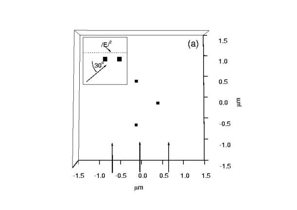
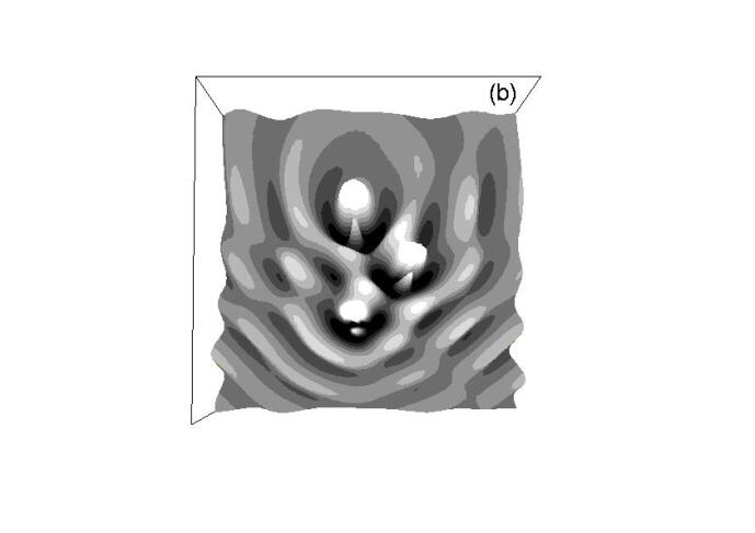
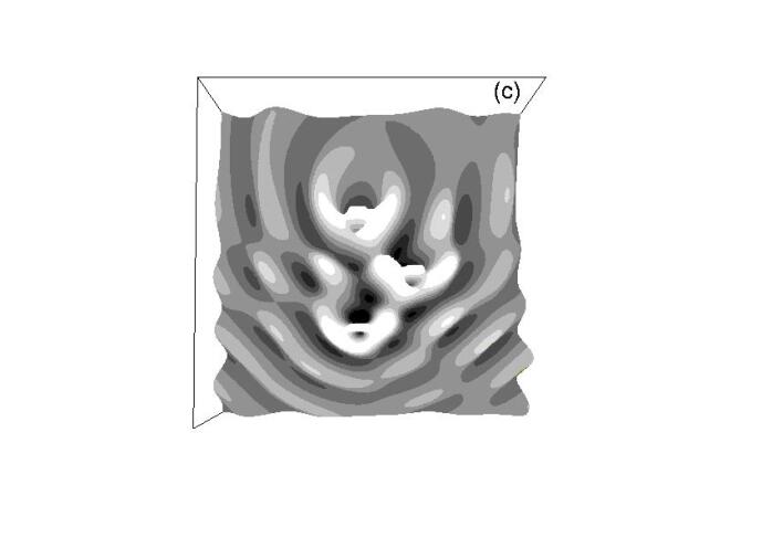
Figure 2: Three cubes of 25nm side length and $\varepsilon=-16.0+1.0i$ in a background of $\varepsilon=1$ illuminated by a p-polarized plane wave of unit amplitude with $\lambda=500{\rm nm}$ from the front and under an angle of $30^{\sf o}$ from beneath the plane defined by the cubes. Setup (a) and electric field intensity $|\vec{E}|^{2}$ calculated via the Born approximation (b) and the exact Green’s functions method (c). Besides subtle differences in the near-field pattern remark that in (b) the grey-scale is from 0.978 to 1.022 whereas in (c) it is from 0.995 to 1.005. The intensity map is taken at a height 25nm above the cubes and given for an area of $3\mu{\rm m}\times 3\mu{\rm m}$.

II.5 System Green’s function and density of states

Adding an arbitrary source term to our original wave equation (1) changes it into

$$-\vec{\nabla}\times\vec{\nabla}\times\vec{E}(\vec{r})+\frac{\omega^{2}}{c^{2}}\varepsilon(\vec{r})\vec{E}(\vec{r})=\vec{Q}(\vec{r}).$$ (12)

If now we know a tensor function $G(\vec{r},\vec{r^{\prime}})$ satisfying

$$-\vec{\nabla}_{\vec{r}}\times\vec{\nabla}_{\vec{r}}\times G(\vec{r},\vec{r^{\prime}})+\frac{\omega^{2}}{c^{2}}\varepsilon(\vec{r})G(\vec{r},\vec{r^{\prime}})={\bf 1}\;\delta(\vec{r}-\vec{r^{\prime}})\quad{\rm or}$$ (13)

$$-\vec{\nabla}_{\vec{r}}\times\vec{\nabla}_{\vec{r}}\times G(\vec{r},\vec{r^{\prime}})+k^{2}G(\vec{r},\vec{r^{\prime}})-V(\vec{r})G(\vec{r},\vec{r^{\prime}})={\bf 1}\;\delta(\vec{r}-\vec{r^{\prime}})$$

then obviously

$$\vec{E}(\vec{r})=\int d^{3}\vec{r^{\prime}}\;G(\vec{r},\vec{r^{\prime}})\;\vec{Q}(\vec{r^{\prime}})$$ (14)

would give a special solution of (12). Any solution of (1) could be added. As generally deduced in section I the implicit relation to get $G$ from is the Dyson equation

$$G(\vec{r},\vec{r^{\prime}})=g(\vec{r},\vec{r^{\prime}})+\int d^{3}\vec{r^{\prime\prime}}\;g(\vec{r},\vec{r^{\prime\prime}})\;V(\vec{r^{\prime\prime}})\;G(\vec{r^{\prime\prime}},\vec{r^{\prime}})$$ (15)

$G(\vec{r},\vec{r^{\prime}})$ for both arguments $\vec{r}$ and $\vec{r^{\prime}}$ covering all space is too much information to display at once and usually much more than what one is interested in. The imaginary part of $G(\vec{r},\vec{r})$ is proportional to the density of states $\rho$ coral ; AD . The deduction of this statement found in quantum mechanics book Calla , however, rather argues with a system of energy eigenstates and the variation of the Green’s function as well as the density of states with energy. No real $\vec{r}$-space is explicitly mentioned. Our interest lies in the spatial dependence of the density of states at fixed light frequency $\omega$.

Even if described in terms of fields, concepts like reactance and work known from electrical circuits may be applied Jac_4 ; circtip . The time average of the work done by the fields is given by

$${\rm Re}\;\frac{1}{2}\int d^{3}\vec{r^{\prime}}\;\vec{J}^{*}(\vec{r^{\prime}})\;\vec{E}(\vec{r^{\prime}})$$ (16)

With no other imposed fields, charges or currents than an oscillating point dipole, the latter will present the only external current $\vec{J}$, which will thus be located as $\delta(\vec{r^{\prime}}-\vec{r})$. If the dipole moment oscillates as $\vec{p}(\vec{r^{\prime}},t)=\vec{p}_{0}e^{-i\omega t}\delta(\vec{r^{\prime}}-\vec{r})$, the corresponding current is $\vec{J}(\vec{r^{\prime}},t)=-i\omega\vec{p}_{0}e^{-i\omega t}\delta(\vec{r^{\prime}}-\vec{r})$. Deducing the wave equation for time harmonic fields (in vacuum for simplicity here) from Maxwells equations with current term

$$\vec{\nabla}\times\vec{E}-i\omega\mu_{0}\vec{H}=0\quad{\rm and}\quad\vec{\nabla}\times\mu_{0}\vec{H}+\varepsilon_{0}\mu_{0}i\omega\vec{E}=\mu_{0}\vec{J}$$

leads to

$$-\vec{\nabla}\times\vec{\nabla}\times\vec{E}+\frac{\omega^{2}}{c^{2}}\vec{E}=-i\omega\mu_{0}\vec{J}$$ (17)

from which we see that the source term for the dipole has to be set as $\vec{Q}(\vec{r^{\prime}})=-i\omega\mu_{0}\vec{J}(\vec{r^{\prime}})=-\omega^{2}\mu_{0}\vec{p}_{0}e^{-i\omega t}\delta(\vec{r^{\prime}}-\vec{r})$. The integral (16) reduces to the value of $\vec{J}^{*}\vec{E}$ at $\vec{r}$. The electric field we get from (14):

$$\vec{E}(\vec{r})=-\omega^{2}\mu_{0}e^{-i\omega t}\int d^{3}\vec{r^{\prime}}\;G(\vec{r},\vec{r^{\prime}})\;\delta(\vec{r^{\prime}}-\vec{r})\;\vec{p}_{0}=-\omega^{2}\mu_{0}e^{-i\omega t}G(\vec{r},\vec{r})\vec{p}_{0}$$

Inserting $\vec{J}^{*}$ and $\vec{E}$ into (16) the time factors cancel as expected for a time average and but for a factor $\omega^{3}\mu_{0}/2$ we get

$${\rm Re}\;i\;\vec{p}_{0}\;G(\vec{r},\vec{r})\;\vec{p}_{0}=-\;{\rm Im}\;\vec{p}_{0}\;G(\vec{r},\vec{r})\;\vec{p}_{0}$$ (18)

Choosing unit vectors along the coordinate axis for the probe dipole $\vec{p}_{0}$, (20) will filter out the trace elements of the matrix $G(\vec{r},\vec{r})$. We associate $\rho_{x}(\vec{r})\propto-{\rm Im}G_{xx}(\vec{r},\vec{r})$, $\rho_{y}(\vec{r})\propto-{\rm Im}G_{yy}(\vec{r},\vec{r})$, $\rho_{z}(\vec{r})\propto-{\rm Im}G_{zz}(\vec{r},\vec{r})$ and a total $\rho(\vec{r})=\rho_{x}(\vec{r})+\rho_{y}(\vec{r})+\rho_{z}(\vec{r})$.

A motivation for taking the negative imaginary part of $G(\vec{r},\vec{r})$ as a measure for the presence of modes can also be obtained by comparison to the energy resonance of a forced oscillator Alonso . For optimal excitation from the energy point of view - in contrast to amplitude resonance - the force has to be $\pi/2$ ahead of the elongation or in phase with the velocity of the oscillator. $G(\vec{r},\vec{r})$ describes the field caused by backaction of the system at the place of the probe dipole moment (taken as reference phase zero), and therefore $-{\rm Im}G(\vec{r},\vec{r})$ is the part that can in a resonant manner further enhance the dipole oscillation. (In reality radiation out of the system will provide strong damping.)

We now intend to evaluate a map of $G(\vec{r},\vec{r})$ on, for example, a horizontal plane. The plane may lie above or below object cells or even cut some. Like the objects, the, of course, finite area of interest on the plane is divided into cells. Just depending on the desired resolution of the map the unit cell length of this mesh may well differ from the cell size chosen to discretize the objects (Fig.1). The list of object cell midpoints $\{\vec{r}_{i}\}$ from the last section, which shall be called region $A$, is extended by all cell midpoints from the map in the plane, which shall be called region $B$ and is now understood to to be included in counting $i$ from 1 to a new $N$. Analogously to (8) the integral in (15) is replaced by a sum:

$$G(\vec{r}_{i},\vec{r}_{k})=g(\vec{r}_{i},\vec{r}_{k})+\sum_{j=1}^{N}\Delta v\;g(\vec{r}_{i},\vec{r}_{j})\;V(\vec{r}_{j})\;G(\vec{r}_{j},\vec{r}_{k})$$ (19)

It does not matter that the map $B$ has a different mesh from $\Delta v$ as for the objects $A$, as $V(\vec{r}_{j})=0$ for $\vec{r}_{j}$ in $B$, anyway. (Spatial overlap of cells from $A$ and $B$ and even coincidence of midpoints is no problem; a place can be counted with $V(\vec{r}_{j})$ in $A$ and without in $B$.)

Although only $G(\vec{r}_{i},\vec{r}_{i})$ with $\vec{r}_{i}$ in region $B$ is wanted as a final result, (21) has to be set up as an equation for a matrix of all $G$ with each of its arguments any cell in $A$ or $B$, schematically sketched as $\begin{pmatrix}\vbox{\halign{\strut# & \vrule\ # \cr AA &AB \cr\hrule\cr BA &BB \cr}}\end{pmatrix}$. To solve (21) for $G$ we have to invert the same kind of matrix as in (8), the only difference being that $j$ now also runs over the plane cells in addition to the object cells.

$$G={\rm M}^{-1}\;g$$ (21a)

$G$ and $g$ are themselves matrices on contrast to vectors $\vec{\vec{E}}$ and $\vec{\vec{E}}_{b}$. $G$ consists of 3x3-blocks $G(\vec{r}_{j},\vec{r}_{k})$, $g$ is made of blocks $g(\vec{r}_{i},\vec{r}_{k})$ and the 3x3-block at position $(i,j)$ in ${\rm M}$ given by ${\bf 1}\delta_{ij}-\Delta v\;g(\vec{r}_{i},\vec{r}_{j})\;V(\vec{r}_{j})$. The $g$ in (21a) and ${\rm M}$ like the big $G$-matrix have the structure $\begin{pmatrix}\vbox{\halign{\strut# & \vrule\ # \cr AA &AB \cr\hrule\cr BA &BB \cr}}\end{pmatrix}$. One could invert ${\rm M}$ as given, for example by the procedure from appendix A. The matrix $M={\bf 1}-{\rm M}$ there is initialized with $gV$. Its $AB$ and $BB$ quadrants are zero and will stay zero throughout the procedure, $M=\begin{pmatrix}\vbox{\halign{\strut# & \vrule\ # \cr AA &0 \cr\hrule\cr BA &0 \cr}}\end{pmatrix}$. This is no contradiction, as it is not ${\rm M}$ that is singular. Quadrant $BA$ will be needed for multiplication with $g$ in (21a). However there is an even more efficient algorithm to get $G$ that already includes the multiplication by $g$. It directly calculates $G=({\bf 1}-gV)^{-1}g$, which is the compact way to write (21a) as the solution of (15), also denoted $G=g+gVG$ for short. The technical details can be found in appendix B.

Figure 3: (a) Top view of the structure: gold pads (90x90x30nm) on a glass subtrate. Calculated densities of states $\rho_{xx}$ (b) $\rho_{yy}$ (c) and $\rho_{zz}$ (d) in a plane 100nm above the substrate for wavelength $\lambda=543{\rm nm}$ [reproduced after Chicel ]. The grey scale is from -50 to 35 in (b), -45 to 30 in (c), -7.5 to 15 in (d) and higher or lower values are white or black, respectively.

Trace components of $G(\vec{r},\vec{r})$ meaning densities of states for the three polarization directions (Fig.3) above an optical coral coral in analogy to a quantum coral Eigler have been measured Chicel in a so called forbidden-light near-field optical microscope forbidden . The sample consists of a stadium arrangement of gold particles on a glass surface. The forbidden-light setup prevents detecting light emitted from the fiber tip that has not passed through surface modes that make up the density of states for this system. Like for antinodal and nodal points in a resonator, more energy can go into the system when the excitation is placed at a point of high density of states than when coupling is bad where the density is low.

II.6 Remarks on the source terms and alternative solutions

In section 4 we saw that it is convenient to start from a solution for the field in the form (7) if the excitation comes, for example, from a background field belonging to a plane wave. Though the matrix to invert bore a certain similarity to the evaluation of the Green’s tensor in section 5, with (8) and (9) we directly calculated the field. In contrast, more adapted to localized sources, there is (14) as a solution of (12). If there is no additional background field to cause any excitation, no solution of the equation (1) with zero right side is to be added as further contribution and (14) is the field distribution to be observed. (14) has to be rewritten in terms of finite elements in order to be used in a numerical calculation. In the same way as the objects the source $\vec{Q}$ has to be devided into discrete cells or elementary dipoles. To distinguish their $L$ locations from those of the objects we shall enumerate them as $\vec{\rho}_{\alpha}$, $\alpha=1,2,\ldots,L$. The place $\vec{r}$ to evaluate the field $\vec{E}$ may be anywhere outside or inside the objects as well as beside or even at a source location. For the following development the Dyson equation for the Green’s tensor is needed in a discretized form for both its variants $G=g+gVG$ and $G=g+GVg$.

$$\vec{E}(\vec{r}) = \sum_{\alpha=1}^{L}G(\vec{r},\vec{\rho}_{\alpha})\vec{Q}(\vec{\rho}_{\alpha})$$ (22a)

$$= \sum_{\alpha=1}^{L}g(\vec{r},\vec{\rho}_{\alpha})\vec{Q}(\vec{\rho}_{\alpha})+\sum_{\alpha=1}^{L}\sum_{j=1}^{N}G(\vec{r},\vec{r}_{j})V(\vec{r}_{j})g(\vec{r}_{j},\vec{\rho}_{\alpha})\vec{Q}(\vec{\rho}_{\alpha})$$

$$= \sum_{\alpha=1}^{L}g(\vec{r},\vec{\rho}_{\alpha})\vec{Q}(\vec{\rho}_{\alpha})+\sum_{\alpha=1}^{L}\sum_{j=1}^{N}g(\vec{r},\vec{r}_{j})V(\vec{r}_{j})g(\vec{r}_{j},\vec{\rho}_{\alpha})\vec{Q}(\vec{\rho}_{\alpha})+$$

$$\sum_{\alpha=1}^{L}\sum_{j=1}^{N}\sum_{i=1}^{N}g(\vec{r},\vec{r}_{i})V(\vec{r}_{i})G(\vec{r}_{i},\vec{r}_{j})V(\vec{r}_{j})g(\vec{r}_{j},\vec{\rho}_{\alpha})\vec{Q}(\vec{\rho}_{\alpha})$$

$$= \sum_{\alpha=1}^{L}g(\vec{r},\vec{\rho}_{\alpha})\vec{Q}(\vec{\rho}_{\alpha})+\sum_{\alpha=1}^{L}\sum_{j=1}^{N}g(\vec{r},\vec{r}_{j})V(\vec{r}_{j})G(\vec{r}_{j},\vec{\rho}_{\alpha})\vec{Q}(\vec{\rho}_{\alpha})$$

$$= \sum_{\alpha=1}^{L}g(\vec{r},\vec{\rho}_{\alpha})\vec{Q}(\vec{\rho}_{\alpha})+\sum_{j=1}^{N}g(\vec{r},\vec{r}_{j})V(\vec{r}_{j})\vec{E}(\vec{r}_{j})$$ (22d)

Having in mind a region where and a resolution with which $\vec{E}(\vec{r})$ is to be evaluated like the discretized plane $B$ from the last section, it would be possible to supply $G$ for all needed combinations of arguments $(\vec{r},\vec{\rho}_{\alpha})$ and calculate $\vec{E}(\vec{r})$ as the single sum from (22a). To weave in the influence of the objects, $G$ would have to be set up as a big matrix like in the last section over all combinations of three regions $A$, $S$ and $B$ here, the objects, the source and the map. Having calculated $G$ in the $A$-$B$-scheme from the last section, one could evaluate $\vec{E}(\vec{r})$ with $G(\vec{r},\vec{r}_{j})$ as written in (22b). However, the most efficient way is given in (22c). $G(\vec{r}_{i},\vec{r}_{j})$ is merely needed for $\vec{r}_{i}$ and $\vec{r}_{j}$ from the set of object cells, keeping a matrix to be inverted as small as possible, namely of $(AA)$-type. Choosing $\vec{r}_{i}$ and $\vec{r}_{k}$ in (21) in the object set $A$, instead of in $A$ or $B$ as the equation was originally set up for, we see that (21) presents a closed system of equations for all such $G(\vec{r}_{i},\vec{r}_{k})$. Then for (22c) more summations over products with $g$-functions, which are analytically known for any pair of arguments, can be considered less demanding in computing time than the inversion of large matrices.

In the transformation from (22c) to (22d) after swapping index names $i$ and $j$ in the last sum, $G=g+GVg$ and (14) have been exploited. Using (22d) for $\vec{E}(\vec{r})$ renders an implicit equation for the field in the form (10) or (10*) from section I. $\vec{E}(\vec{r})$ is the equivalent of $\phi_{ihq}$ and as stated earlier, we assume that physically there is no background field $\phi_{0}$ that could initiate an additional field distribution $\phi_{ih}$. Although not very convenient, a plane wave as exciting field could be understood as stemming from a sufficiently long and dense array of Huygens elementary dipole sources $\vec{Q}$ reasonably far away from the objects. The other way round, for a single dipole source or a number of dipole sources distributed in space the field they would produce at any location $\vec{r}$ in homogeneous space is the superposition of their individual fields, and putting $\vec{E}_{b}(\vec{r})=\sum_{\alpha=1}^{L}g(\vec{r},\vec{\rho}_{\alpha})\vec{Q}(\vec{\rho}_{\alpha})$ the ansatz (7) can be used also for this case.

Like the field $\vec{E}$ anywhere was obtained as a straight-forward summation once having its values at the places of the object cells, finally an alternative way to the procedure from the last section to get the Green’s tensor $G$ shall be given, also requiring only the inversion of a matrix with size the number of object cells. Series expansion is used to rewrite the solution of the Dyson equation:

$$G = ({\bf 1}-gV)^{-1}g=[{\bf 1}+\sum_{n=1}^{\infty}(gV)^{n}]g=g+gV(\sum_{n=0}^{\infty}(gV)^{n})g$$

$$= g+gV({\bf 1}-gV)^{-1}g$$

$$= g+gVg+gV(\sum_{n=0}^{\infty}(gV)^{n})gVg=g+gVg+gV\;({\bf 1}-gV)^{-1}g\;Vg$$

$$= g+gVg+gVGVg$$ (23b)

Designating regions the spatial arguments belong to on (23a) we get for $G_{BB}$:

$$G_{BB}=g_{BB}+g_{BA}\;V_{A}\;({\bf 1}-gV)^{-1}_{AA}\;g_{AB},$$ (23a’)

As $V$ does not vanish only in region $A$, the first index of $({\bf 1}-gV)^{-1}$ obviously must be $A$. $({\bf 1}-gV)^{-1}$ being $\sum_{n=0}^{\infty}(gV)^{n}$, for power zero the second region index automatically is the same as the first and all other powers ending with $V$ imply second index $A$. It is sufficient to set up the matrix ${\bf 1}-gV$ as an $(AA)$-block and invert that. Should one prefer to evaluate a complete $G$, which differs from the above inverted matrix by a factor $g$, line (23b) like (22c) shows that it is in principle only necessary to get $G$ from some self-consistent implicit equation in the object region $A$. $G_{AA}$ can be constructed applying the procedure described in appendix B to a matrix set up as $(AA)$-block only. The inversion has to be completed in this case, though. Going through the diagonal elements, all lines and columns have to be updated in each step, including the ones above and to the left of as well as the ones the respective diagonal element is in. Writing (23b)

$$G_{BB}=g_{BB}+g_{BA}\;V_{A}\;g_{AB}+g_{BA}\,V_{A}\,G_{AA}\;V_{A}\;g_{AB}$$ (23b’)

as summation over discrete elements ready for use in a calculation then reads:

$$G(\vec{r},\vec{r^{\prime}})=g(\vec{r},\vec{r^{\prime}}) + \sum_{j=1}^{N}g(\vec{r},\vec{r}_{j})\;V(\vec{r}_{j})\;g(\vec{r}_{j},\vec{r^{\prime}})$$ (23b”)

$$+ \sum_{j=1}^{N}\sum_{i=1}^{N}g(\vec{r},\vec{r}_{j})\;V(\vec{r}_{j})\;G(\vec{r}_{j},\vec{r}_{i})\;V(\vec{r}_{i})\;g(\vec{r}_{i},\vec{r^{\prime}})$$

Of course, summations run over all object cells here. No numerical advantage can be drawn out of $\vec{r^{\prime}}=\vec{r}$ in (23b”). With the same effort of making $G_{AA}$ it can be used to evaluate maps of $G(\vec{r},\vec{r})$ as well as plots of $G(\vec{r},\vec{r^{\prime}})$ with $\vec{r^{\prime}}$ fixed or even some function of $\vec{r}$.

II.7 Conclusions and Outlook for section II

We have presented a method to solve the problem of scattering of electromagnetic waves off an arbitrary distribution of dielectric objects, that is the exact evaluation of the field, especially in the near zone where higher-order multiple reflections can become important. Besides the field distribution we have obtained the Green’s tensor characterizing the system independently from the form of the excitation. It represents the response function and also the density of states for supported electric fields.

For a methodical introduction we have restricted our considerations to dielectric materials and the electric field. Without magnetic susceptibilities the magnetic field distribution can be calculated once having the electric field inside the objets by a formula like (9) with the magnetic background field and replacing $g$ by a tensor including the conversion from the electric to the magnetic field by taking the rotation Girard . It is further possible to treat non-uniform magnetic permeabilities and even mixed systems with dielectric and magnetic objects EPJel . The electric Green’s tensor presented above is then paired by a magnetic counterpart and genuine mixed response functions also exist. Whereas the calculation of the field distributions even for mixed systems is quite straight forward, the construction of the Green’s tensor is more involved. It lives of the idea of handling one kind of objects first and then considering this setup as the background to include the other kind. There is no approximation or ranking in importance in this procedure.

The discussion here has only considered finite objects in a homogeneous background as well as cartesian coordinates where vector and tensor components have been written out. Cylindrical and spherical coordinates are also commonly used Chew ; ellipse and the Green’s functins formalism has been developped for layered media MarLith ; Chew ; stratified . Besides wave-guide applications the use for modelling typical near-field optics experiments, where the microstructures to investigate are prepared on a substrate surface, lies in putting the influence of this surface into a background Green’s tensor Girard ; AD which is then implied the way we used $g$ here.

Details of applications of the Green’s functions technique in electrodynamics to more complicated situations as well as beautiful results of corresponding experiments can be found in the given references. This text focussed on calculation techniques and further intended to give an overview of slightly different formal ways to calculate Green’s tensors and fields of which either may be optimal for a specific problem.

Appendix A: an unusual matrix inversion

Suppose a complex quadratical matrix to invert is already given in the form ${\rm M}={\bf 1}-M={\bf 1}-(m)_{ij}$ or if it is not, we rewrite it like that. There is no restriction on the values of the numbers $m_{ij}$. To get the inverted matrix proceed as follows: Of matrix $M$ one by one take the diagonal elements $m_{ii}$ and to all elements $m_{ab}$ add $m_{ai}(1-m_{ii})^{-1}m_{ib}$. After having worked through the matrix for one such $m_{ii}$, the changed matrix values have to be taken to do so for the next, also already changed, diagonal element. Obviously $N$ such steps are required for an $N\times N$-matrix. This will yield $({\bf 1}-M)^{-1}-{\bf 1}$, such that in the end 1 has to be added to all diagonal elements in order to obtain $({\bf 1}-M)^{-1}$. For clearness we write out the first two transformation steps of the matrix:

$$\begin{pmatrix}m_{11}&m_{22}&\cr m_{21}&m_{22}&\cr&&\ddots\cr\end{pmatrix}\rightarrow\begin{pmatrix}m_{11}+m_{11}(1-m_{11})^{-1}m_{11}&m_{12}+m_{11}(1-m_{11})^{-1}m_{12}\cr m_{21}+m_{21}(1-m_{11})^{-1}m_{11}&m_{22}+m_{21}(1-m_{11})^{-1}m_{12}\cr\end{pmatrix}$$

$$\rightarrow\begin{pmatrix}m_{11}+m_{11}(1-m_{11})^{-1}m_{11}+&m_{12}+m_{11}(1-m_{11})^{-1}m_{12}+\cr(m_{12}+m_{11}(1-m_{11})^{-1}m_{12})\cdot&(m_{12}+m_{11}(1-m_{11})^{-1}m_{12})\cdot\cr(1-m_{22}-m_{21}(1-m_{11})^{-1}m_{12})^{-1}&(1-m_{22}-m_{21}(1-m_{11})^{-1}m_{12})^{-1}\cr\cdot(m_{21}+m_{21}(1-m_{11})^{-1}m_{11})&\cdot(m_{22}+m_{21}(1-m_{11})^{-1}m_{12})\cr&\cr m_{21}+m_{21}(1-m_{11})^{-1}m_{11}+&m_{22}+m_{21}(1-m_{11})^{-1}m_{12}+\cr(m_{22}+m_{21}(1-m_{11})^{-1}m_{12})\cdot&(m_{22}+m_{21}(1-m_{11})^{-1}m_{12})\cdot\cr(1-m_{22}-m_{21}(1-m_{11})^{-1}m_{12})^{-1}&(1-m_{22}-m_{21}(1-m_{11})^{-1}m_{12})^{-1}\cr\cdot(m_{21}+m_{21}(1-m_{11})^{-1}m_{11})&\cdot(m_{22}+m_{21}(1-m_{11})^{-1}m_{12})\cr\end{pmatrix}\rightarrow\ldots$$

The inverted matrix $({\bf 1}-M)^{-1}$ can be represented as a geometric series:

$$({\bf 1}-M)^{-1}={\bf 1}+M+M^{2}+\ldots$$ (25)

Truncating and using the sum from the right side is only possible if the series converges whereas the closed form on the left is valid in any case. In contrast to the infinite sum on the right side of (25), our inversion procedure consists in a finite number of steps of adding contributions to the matrix elements. Nevertheless, (25) tells us that the invers $({\bf 1}-M)^{-1}$ is the sum of all powers of $M$ and thus each element in row $a$ and column $b$ must be the sum of all possible products $m_{an_{1}}m_{n_{1}n_{2}}m_{n_{2}n_{3}}\ldots m_{n_{j-1}n_{j}}m_{n_{j}b}$ with any number $j$ of inner indices including none. (Diagonal elements get an extra +1.) There are $N$ different indices $n_{i}$ and they may repeat, of course. Considering that $(1-m_{ii})^{-1}$ can also be written as

$$(1-m_{ii})^{-1}=1+m_{ii}+m_{ii}^{2}+\ldots=1+m_{ii}+m_{ii}m_{ii}+\ldots$$

we see that the first step in (24) adds to each matrix element $m_{ab}$ the sum of all products $m_{a1}m_{11}m_{11}\ldots m_{11}m_{1b}$. In these at least one pair of indices 1 is squeezed between $a$ and $b$ as in $m_{a1}m_{1b}$, the contribution $m_{ab}$ was already there. In the second step all products $m_{a\nu_{1}}m_{\nu_{1}\nu_{2}}\ldots m_{\nu_{\alpha}2}m_{2\nu_{\beta}}\ldots m_{\nu_{j-1}\nu_{j}}m_{\nu_{j}b}$ with $\nu_{1}\nu_{2}\ldots\nu_{j-1}\nu_{j}$ every possible sequence of 1s and 2s will be added. The products with only indices 1 between $a$ and $b$ were there before. In the third step every sequence of indices 1, 2 and 3 with at least one 3-link is added. And so on until in the end at each matrix position between outer indices $a$ and $b$ we have created all possible sequences of an endless game of dominos $m_{ij}$ with numbers $i$ and $j$ from 1 to $N$. This argument was to proove that the result of (24) indeed gives $({\bf 1}-M)^{-1}-{\bf 1}$. We calculate a finite number of $(1-m_{ii})^{-1}$ or products $m_{ai}(1-m_{ii})^{-1}m_{ib}$. The sequence on the right side of (25) need not converge and the original entries in $M$ need not at all be small compared to 1 in their absolute values. There is no approximation in the sense of a perturbation theory. If the matrix ${\bf 1}-M$ is degenerate, the failure of the inversion will be noticed when a value $1-m_{ii}$ becomes zero at some step. Not to confuse notation, remark that in (24) and in products in the text like $m_{a1}m_{11}\ldots m_{1b}$ letters $m$ meant the original matrix entries whereas in expressions $1-m_{ii}$, $(1-m_{ii})^{-1}$ and $m_{ai}(1-m_{ii})^{-1}m_{ib}$ we referred to the entries at the respective step of the matrix transformation.

In the application from the main text $i=1,\ldots,N$ enumerates the object cells. At position $(i,j)$ in $({\bf 1}-gV)^{-1}$ when expanded into a series having every possible sequence $g(\vec{r}_{n_{1}},\vec{r}_{n_{2}})V(\vec{r}_{n_{2}})g(\vec{r}_{n_{2}},\vec{r}_{n_{3}})V(\vec{r}_{n_{3}})g\ldots g(\vec{r}_{n_{j-1}},\vec{r}_{n_{j}})V(\vec{r}_{n_{j}})$ shows that the resulting field at any place (inside or outside the objects) is the interference of the background field and the fields reradiated by all the object dipoles having undergone every possible scattering path between the objects (Fig.1). A complication in the electrodynamics application at this stage is the fact that each matrix element $m$ actually in itself is a 3x3 matrix indicating the effect of three field components at one place onto three field components at a another place. $g$ on the discrete space of the objects can be written blockwise with a scheme of quadruple indices

$V(\vec{r}_{k})$ in the product $g(\vec{r}_{i},\vec{r}_{k})V(\vec{r}_{k})$ just multiplies the respective column.

One could use the inversion procedure working off the diagonal elements marked by ovals, requiring $3N$ steps then. However, the process is equally applicable to 3x3 blocks as marked by the dashed rectangles, since by its dimension the whole matrix can be divided up into 3x3-blocks. Then $({\bf 1}-m_{ii})^{-1}$ means the inversion of a 3x3 matrix and $m_{ai}({\bf 1}-m_{ii})^{-1}m_{ib}$ to update the blocks means the product of three 3x3 matrices. These operations should be programmed as elementary procedures.

The given procedure to invert a matrix can become of advantage if for sparse matrices conventional routines run into numerical difficulties because of many zero values. Besides that, it can be adapted to become quite efficient if only parts of the inverted matrix are needed or for symmetry reasons it is known that blocks or patterns of matrix elements vanish and will stay zero throughout the inversion. Although for the calculation of the Green’s tensor a slightly modified procedure is applied that directly optimizes the numerical solution of the Dyson equation (see appendix B), the matrix inversion was discussed here, because it may be used for more general purposes and in other contexts as well.

Appendix B: Calculating the Green’s tensor

In the following instructions are given how to calculate the Green’s tensor

$$G=({\bf 1}-gV)^{-1}g=g+gVg+gVgVg+\ldots$$ (21)

being efficient in the way that finally only $G(\vec{r},\vec{r})$ of equal arguments on the mesh points of map $B$ need to have the correct values priv ; EPJel . For a start nevertheless consider that $G(\vec{r}_{i},\vec{r}_{k})$ with arguments $\vec{r}_{i}$ and $\vec{r}_{k}$ from the big set of all object and map cell midpoints will have to be the sum of all products

$$g(\vec{r}_{i},\vec{r}_{n_{1}})V(\vec{r}_{n_{1}})g(\vec{r}_{n_{1}},\vec{r}_{n_{2}})V(\vec{r}_{n_{2}})g(\vec{r}_{n_{2}},\vec{r}_{n_{3}})\ldots V(\vec{r}_{n_{j-1}},\vec{r}_{n_{j}})g(\vec{r}_{n_{j}},\vec{r}_{k}).$$

$\vec{r}_{n_{1}}$, $\vec{r}_{n_{2}}$, $\ldots$, $\vec{r}_{n_{j}}$ can only be object cells and any sequence of them has to be created, including the empty one with no $V$ giving the term $g(\vec{r}_{i},\vec{r}_{k})$. Initiate a matrix $\begin{pmatrix}\vbox{\halign{\strut# & \vrule\ # \cr AA &AB \cr\hrule\cr BA &{\tiny\vbox{\halign{\strut# & # & # \cr BB &&\cr&$\ddots$ &\cr&&BB \cr}} } \cr}}\end{pmatrix}$ - for simplicity call it $G$ from the beginning - with line and column arguments running over all object cells in $A$ and all map cells in $B$ with $g(\vec{r}_{i},\vec{r}_{k})$ in each 3x3-subblock. In the $BB$-quadrant only diagonal blocks $g(\vec{r}_{i},\vec{r}_{i})$ will be needed, however. Work off the diagonal subblocks through the $AA$-quadrant. For the $n$th one prepare the inverted 3x3-matrix $({\bf 1}-G(\vec{r}_{n},\vec{r}_{n})V(\vec{r}_{n}))^{-1}$ and to all entries from line $n+1$ and column $n+1$ on add the product given below.

$$G(\vec{r}_{i},\vec{r}_{k})\rightarrow G(\vec{r}_{i},\vec{r}_{k})+G(\vec{r}_{i},\vec{r}_{n})\;V(\vec{r}_{n})\;({\bf 1}-G(\vec{r}_{n},\vec{r}_{n})V(\vec{r}_{n}))^{-1}\;G(\vec{r}_{n},\vec{r}_{k})$$ (26)

In the following step use the updated entries in the above recipe. In the $n$th step you need not update entries in line $n$ or above or in column $n$ or to the left of it, because these will not be needed as multiplication factors $G(\vec{r}_{i},\vec{r}_{m})$ and $G(\vec{r}_{m},\vec{r}_{k})$ for $m>n$ any more. The parts of quadrants $AB$ and $BA$ remaining after these restrictions have to be changed by (26) for every $n$. Merely diagonal 3x3 blocks have to be done in the $BB$-quadrant. The first step adds all products consisting of any non-zero number of factors $V(\vec{r}_{1})$ between $g$s, the second step all products eventually containing $V(\vec{r}_{1})$ and one up to any number of $V(\vec{r}_{2})$, and so on. The procedure is finished after $\vec{r}_{n}$ has run down the diagonal of the $AA$-quadrant. All sequences of multiple scattering from the objects are then included.

We could have filled the whole $BB$-quadrant with initial $g_{BB}$ 3x3-blocks and updated the entire $BB$-quadrant in each step. Like in the matrix inversion procedure from appendix A we should further have worked down the complete diagonal and done (26) for every $\vec{r}_{n}$ from region $B$ as well. There will, however, be no additions as $V(\vec{r}_{n})=0$ for $\vec{r}_{n}$ in $B$ (even if a map cell accidently coincides with an object cell). This argument also reveals why non-diagonal elements in $BB$ do not have to be evaluated. They can never appear as multiplication factors $G(\vec{r}_{i},\vec{r}_{n})$ or $G(\vec{r}_{n},\vec{r}_{k})$. The $BB$ diagonal is the resulting $G(\vec{r},\vec{r})$-map we wanted.

Initiating the matrix by $g$ and introducing the $V$ on treating the respective diagonal element makes the outcome of the procedure directly $({\bf 1}-gV)^{-1}g$ compared to initiating the matrix with $gV$ and as an intermediate step obtaining $({\bf 1}-gV)^{-1}$.

III All-order quantum transport

It is demonstrated how the transport problem for two open free-electron gas reservoirs with arbitrary coupling can be solved by finding the system’s Green’s function. In this sense the article is an introduction on Green’s functions for treating interaction. A very detailed discussion of the current formula is given on an elementary basis. Despite formal resemblances the stationary transport situation, however, differs in its nature from introducing coupling between energy levels in a closed system where then the interest lies in modified eigenvalues and eigenstates.

III.1 Introduction

By modern lithography techniques so-called point contacts Agrait can be arranged between conductors. These have sufficiently small dimensions such that electronic modes get quantized. However, coupling across such constrictions need not be so weak as to be described by a small tunnel probability, but can be influenced by coherent interference of multiple reflections. Point contacts can be obtained by indenting STM-tips into some material RubioSTM , electromigration herre or the break-junction technique break . Whereas for constrictions imposed by gate electrodes to a two-dimensional electron gas in semiconductors vanWees one observes quantized conductance values in the sense of fully transmitting or totally switched-off modes, the application in mind behind this work is the type of connection like the single-atom contact, characterized by an ensemble of channels buett , which can also have intermediate transmission amplitudes between zero and one Sche97 . Even with some fully transmitting modes the contact bears a resistance in the order of the quantum resistances $R_{k}=h/e^{2}=26k\Omega$ SCT , such that viewing the system as a left and a right side with some interaction is an appropriate picture. Furthermore contributions from several channels just add in the current. Although a transmitting channel in a point contact is the application in mind, this article shows how to set up a general procedure to solve the problem of transport for two open reservoirs with more or less strong coupling between them, and thus how the Green’s functions formalism from section I is implied in an area of current research aktuel_1 ; aktuel_2 .

III.2 Green’s functions formalism

As a preparation, consider systems like, for example, the bulk material on the left or the right side (Fig.1a) without coupling. For these we suppose that we know the Hamiltonian $H^{0}$ and the wave function $\Psi^{0}$ at any given energy $\hbar\omega$ satisfying the Schrödinger equation. Denoting the Hamiltonians $H_{LL}=H_{RR}=H^{0}$ (doubling the index makes sense later), the wave functions $\Psi_{L}^{0}=\Psi_{R}^{0}=\Psi^{0}$ and the time derivative as $\partial_{\tau}$, the Schrödinger equations for both sides - for the moment just formally put into matrix form - are

$$\begin{pmatrix}i\hbar\partial_{\tau}-H_{LL}&0\cr 0&i\hbar\partial_{\tau}-H_{RR}\cr\end{pmatrix}\begin{pmatrix}\Psi^{0}_{L}(\tau)\cr\Psi^{0}_{R}(\tau)\cr\end{pmatrix}=\begin{pmatrix}0\cr 0\cr\end{pmatrix}$$ (1)

Corresponding to this differential equation we have the Green’s functions equation

$$\begin{pmatrix}i\hbar\partial_{\tau}-H_{LL}&0\cr 0&i\hbar\partial_{\tau}-H_{RR}\cr\end{pmatrix}\begin{pmatrix}g_{LL}(\tau,\tau^{\prime})&0\cr 0&g_{RR}(\tau,\tau^{\prime})\cr\end{pmatrix}=\begin{pmatrix}\delta(\tau-\tau^{\prime})&0\cr 0&\delta(\tau-\tau^{\prime})\cr\end{pmatrix}$$

If we knew $g=g_{LL}=g_{RR}$, we could immediately also give a solution to (1) with a source term added

$$\begin{pmatrix}i\hbar\partial_{\tau}-H_{LL}&0\cr 0&i\hbar\partial_{\tau}-H_{RR}\cr\end{pmatrix}\begin{pmatrix}\Psi^{q}_{L}(\tau)\cr\Psi^{q}_{R}(\tau)\cr\end{pmatrix}=\begin{pmatrix}Q_{L}(\tau)\cr Q_{R}(\tau)\cr\end{pmatrix}$$ (3)

namely

$$\begin{pmatrix}\Psi^{q}_{L}(\tau)\cr\Psi^{q}_{R}(\tau)\cr\end{pmatrix}=\int d\tau^{\prime}\;\begin{pmatrix}g_{LL}(\tau,\tau^{\prime})&0\cr 0&g_{RR}(\tau,\tau^{\prime})\end{pmatrix}\;\begin{pmatrix}Q_{L}(\tau^{\prime})\cr Q_{R}(\tau^{\prime})\cr\end{pmatrix}$$ (4)

However, we are more interested in the solution when an interaction between left and right is present, expressed through coupling Hamiltonians $H_{LR}$ and $H_{RL}$,

$$\begin{pmatrix}i\hbar\partial_{\tau}-H_{LL}&-H_{LR}\cr-H_{RL}&i\hbar\partial_{\tau}-H_{RR}\cr\end{pmatrix}\begin{pmatrix}\Psi_{L}(\tau)\cr\Psi_{R}(\tau)\cr\end{pmatrix}=\begin{pmatrix}0\cr 0\cr\end{pmatrix}$$ (5)

and we shall refer to this case by $\Psi$ without upper index. Introducing the coupling, of course, was the motivation for writing the Schrödinger equation in matrix form over the site space consisting of L(left) and R(right). Putting the coupling terms on the right side of the equation, they mimic a source

$$\begin{pmatrix}i\hbar\partial_{\tau}-H_{LL}&0\cr 0&i\hbar\partial_{\tau}-H_{RR}\cr\end{pmatrix}\begin{pmatrix}\Psi_{L}(\tau)\cr\Psi_{R}(\tau)\cr\end{pmatrix}=\begin{pmatrix}0&H_{LR}\cr H_{RL}&0\cr\end{pmatrix}\begin{pmatrix}\Psi_{L}(\tau)\cr\Psi_{R}(\tau)\cr\end{pmatrix}$$ (6)

and following (4) the solution can formally be written as

$$\begin{pmatrix}\Psi_{L}(\tau)\cr\Psi_{R}(\tau)\cr\end{pmatrix}=\int d\tau^{\prime}\;\begin{pmatrix}g_{LL}(\tau,\tau^{\prime})&0\cr 0&g_{RR}(\tau,\tau^{\prime})\end{pmatrix}\begin{pmatrix}0&H_{LR}\cr H_{RL}&0\cr\end{pmatrix}\begin{pmatrix}\Psi_{L}(\tau^{\prime})\cr\Psi_{R}(\tau^{\prime})\cr\end{pmatrix}$$

obtaining the implicit Lippmann-Schwinger equation for the wave functions. Although for the coupled system we do not expect the eigenvectors of $\begin{pmatrix}H_{LL}&H_{LR}\cr H_{RL}&H_{RR}\cr\end{pmatrix}$ to be one with only an upper component localized on the left and one with only a lower component localized on the right, it is convenient to denote these solutions as vectors $\begin{pmatrix}\Psi_{L}\cr\Psi_{R}\cr\end{pmatrix}$, keeping indices L and R. In contrast to section II, where the Lippmann-Schwinger equation was solved in a discretized form to obtain field distributions, for our purposes here (7) will merely serve as a formal step in the derivation of the Green’s function. What we are precisely interested in from a physical point of view is the current that will flow between the left and the right side, and not necessarily explicitly evaluating the wave functions.

The Green’s function $G$ of the coupled system is inferred from an equation analogous to (5), namely

$$\begin{pmatrix}i\hbar\partial_{\tau}-H_{LL}&-H_{LR}\cr-H_{RL}&i\hbar\partial_{\tau}-H_{RR}\cr\end{pmatrix}\begin{pmatrix}G_{LL}(\tau,\tau^{\prime})&G_{LR}(\tau,\tau^{\prime})\cr G_{RL}(\tau,\tau^{\prime})&G_{RR}(\tau,\tau^{\prime})\cr\end{pmatrix}=\begin{pmatrix}\delta(\tau-\tau^{\prime})&0\cr 0&\delta(\tau-\tau^{\prime})\cr\end{pmatrix}$$

$G$ like the Hamiltonian is a full matrix in site space. With $G$, a solution of

$$\begin{pmatrix}i\hbar\partial_{\tau}-H_{LL}&-H_{LR}\cr-H_{RL}&i\hbar\partial_{\tau}-H_{RR}\cr\end{pmatrix}\begin{pmatrix}\Psi^{cq}_{L}(\tau)\cr\Psi^{cq}_{R}(\tau)\cr\end{pmatrix}=\begin{pmatrix}Q_{L}(\tau)\cr Q_{R}(\tau)\cr\end{pmatrix}$$ (9)

would read

$$\begin{pmatrix}\Psi^{cq}_{L}(\tau)\cr\Psi^{cq}_{R}(\tau)\cr\end{pmatrix}=\int d\tau^{\prime}\;\begin{pmatrix}G_{LL}(\tau,\tau^{\prime})&G_{LR}(\tau,\tau^{\prime})\cr G_{RL}(\tau,\tau^{\prime})&G_{RR}(\tau,\tau^{\prime})\cr\end{pmatrix}\begin{pmatrix}Q_{L}(\tau^{\prime})\cr Q_{R}(\tau^{\prime})\cr\end{pmatrix}$$ (10)

where the index cq stands for coupling and source. As explained in section I, we could also have set up a Lippmann-Schwinger equation for $\Psi^{cq}$ as

$$\begin{pmatrix}\Psi^{cq}_{L}(\tau)\cr\Psi^{cq}_{R}(\tau)\cr\end{pmatrix} = \int d\tau^{\prime}\;\begin{pmatrix}g_{LL}(\tau,\tau^{\prime})&0\cr 0&g_{RR}(\tau,\tau^{\prime})\end{pmatrix}\begin{pmatrix}Q_{L}(\tau^{\prime})\cr Q_{R}(\tau^{\prime})\cr\end{pmatrix}+$$

$$\int d\tau^{\prime}\;\begin{pmatrix}g_{LL}(\tau,\tau^{\prime})&0\cr 0&g_{RR}(\tau,\tau^{\prime})\end{pmatrix}\begin{pmatrix}0&H_{LR}\cr H_{RL}&0\cr\end{pmatrix}\begin{pmatrix}\Psi^{cq}_{L}(\tau^{\prime})\cr\Psi^{cq}_{R}(\tau^{\prime})\end{pmatrix}$$

Now from inserting (10) into (11) and for $Q$ choosing some $\delta(\tau^{\prime}-\tau_{0})$ either in the L- or in the R-component the Dyson equation for $G$ is obtained:

$$\begin{pmatrix}G_{LL}(\tau,\tau^{\prime})&G_{LR}(\tau,\tau^{\prime})\cr G_{RL}(\tau,\tau^{\prime})&G_{RR}(\tau,\tau^{\prime})\cr\end{pmatrix}=\begin{pmatrix}g_{LL}(\tau,\tau^{\prime})&0\cr 0&g_{RR}(\tau,\tau^{\prime})\cr\end{pmatrix}+$$

$$\int d\tau^{\prime\prime}\;\begin{pmatrix}g_{LL}(\tau,\tau^{\prime\prime})&0\cr 0&g_{RR}(\tau,\tau^{\prime\prime})\cr\end{pmatrix}\underbrace{\begin{pmatrix}0&H_{LR}\cr H_{RL}&0\cr\end{pmatrix}}_{\sigma}\begin{pmatrix}G_{LL}(\tau^{\prime\prime},\tau^{\prime})&G_{LR}(\tau^{\prime\prime},\tau^{\prime})\cr G_{RL}(\tau^{\prime\prime},\tau^{\prime})&G_{RR}(\tau^{\prime\prime},\tau^{\prime})\cr\end{pmatrix}$$

III.3 Explicit Green’s functions in time and frequency domain

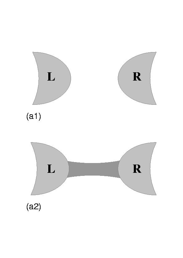
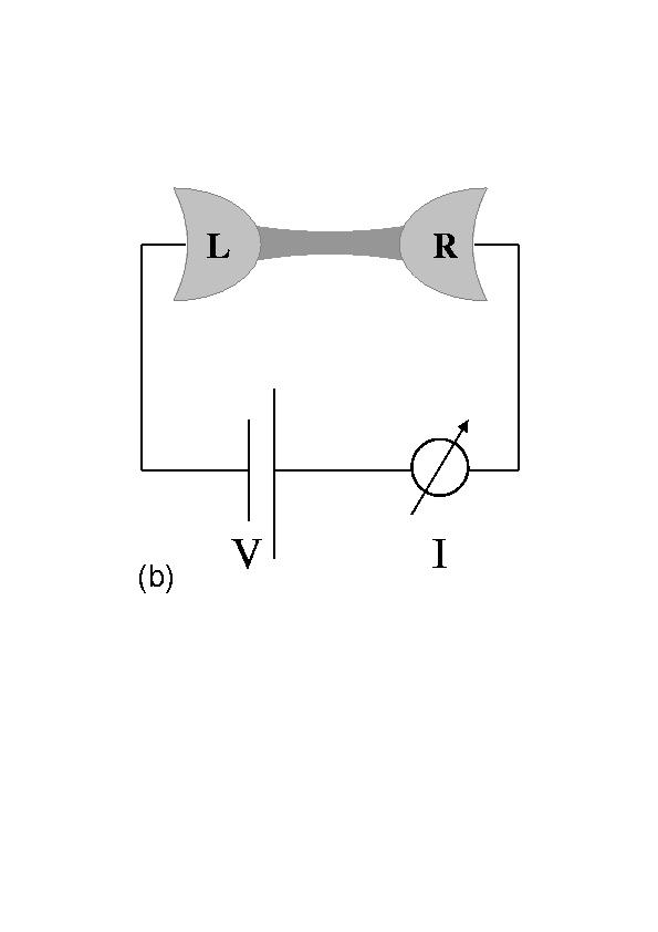
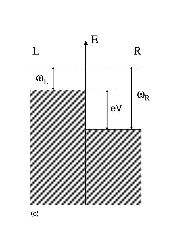
Figure 4: A left and a right bulk reservoir, uncoupled (a1) and coupled (a2). (b) Contact as embedded in a circuit. (c) Fermi levels left and right with applied voltage. The dotted line marks a fixed energy over both sides.

The reservoirs on the left and right being bulk metal, the differential operator of the homogeneous differential equation (1) is given by the free-partical Hamiltonian

$$i\hbar\partial_{\tau}-H^{0}=i\hbar\partial_{\tau}+\frac{\hbar^{2}}{2m}\Delta$$ (13)

and the corresponding wave functions are $\Psi^{0}=e^{\pm i\vec{k}\vec{r}-i\omega\tau}$ according to the dispersion relation $E=\hbar\omega=\frac{\hbar^{2}}{2m}\vec{k}^{2}$. Looking for a Green’s function at given frequency $\omega$, in (2) we can replace $H^{0}$ by $\hbar\omega$ and thus have to solve

$$(i\hbar\partial_{\tau}-\hbar\omega)\;g(\tau,\tau^{\prime},\omega)=\delta(\tau-\tau^{\prime})$$ (14)

We need an expression, the derivative of which produces $\delta(\tau-\tau^{\prime})$. One easily verifies that (14) is satisfied by either

$$g^{r}(\tau,\tau^{\prime},\omega) = -\frac{i}{\hbar}\;\theta(\tau-\tau^{\prime})\;e^{-i\omega(\tau-\tau^{\prime})}$$ (15a)

$$g^{a}(\tau,\tau^{\prime},\omega) = \frac{i}{\hbar}\;\theta(\tau^{\prime}-\tau)\;e^{-i\omega(\tau-\tau^{\prime})}$$ (15b)

The retarded function $g^{r}$ only exists for $\tau\geq\tau^{\prime}$ and the advanced function $g^{a}$ for $\tau\leq\tau^{\prime}$. In (14) for simplicity we restricted ourselves to a single energy and therefore (15) still contain $\omega$ as a parameter. For complete Green’s functions in the time domain these terms have to be multiplied by the density of states $\mathcal{D}(\omega)$ and integrated over energy. Later in transport we shall be interested in the amount of charge transferred, not resolving any more, which energy levels contributions came from. Thinking physically of a small contact between two metallic leads one might argue that in the constriction transverse $k$-vectors are quantized and a one-dimensional continuous density of states remains. Nevertheless, for not too high voltages only a certain energy range around the Fermi energy will play a role in transport and thus setting the density of states equal to its value at the Fermi energy is a good approximation. Anyway, a constant density of states $\mathcal{D}(\omega)=\mathcal{D}$ with occupied states below and empty ones above the Fermi level for each side, left and right, shall just enter our model here as an assumption. We are led to the following representations of the retarded and advanced Green’s functions:

$$g^{r}(\tau,\tau^{\prime})\; = -\frac{i}{\hbar}\;\theta(\tau-\tau^{\prime})\int d\omega\;\frac{\mathcal{D}(\omega)}{2\pi}\;e^{-i\omega(\tau-\tau^{\prime})}$$ (16a)

$$\widehat{=} \frac{\mathcal{D}}{h}\int d\omega\;g^{r}(\omega)\;e^{-i\omega(\tau-\tau^{\prime})}\quad{\rm with}\quad g^{r}(\omega)=-i$$

$$g^{a}(\tau,\tau^{\prime})\; \widehat{=} \frac{\mathcal{D}}{h}\int d\omega\;g^{a}(\omega)\;e^{-i\omega(\tau-\tau^{\prime})}\quad{\rm with}\quad g^{a}(\omega)=i$$ (16b)

Taking out the factor $\mathcal{D}/h$, we get the dimensionless functions $g^{r}(\omega)=-i$ and $g^{a}(\omega)=i$ in frequency space. Remark that their deduction here did not consist in calculating a Fourier transformation. The phase factor $e^{-i\omega(\tau-\tau^{\prime})}$ was already there in (15). The $\omega$-integrals from (16) will be implemented as a useful representation of $g^{r/a}$ still in the time domain. The $\theta$-functions have been deliberately skipped after the $\widehat{=}$-signs. We shall however see that $g^{r}$ and $g^{a}$ finally only appear with the correct relation between their first and second time argument. The $\omega$-integral should indeed be understood as summing over all energies and, even if $g^{r/a}(\omega)$ is a constant, on no account be interpreted as this constant times $2\pi\delta(\tau-\tau^{\prime})$. $e^{-i\omega(\tau-\tau^{\prime})}=e^{-i\omega\tau}\cdot(e^{-i\omega\tau^{\prime}})^{*}=|\Psi^{0}(\tau)><\Psi^{0}(\tau^{\prime})|$ is the projection-like conversion of the phase unit vector of an oscillation from time $\tau^{\prime}$ to time $\tau$. Left(L) and right(R) are distinguished as the origins of wave functions constituting our basis of states, but the junction is considered point-like, that is $\vec{r}=0$ for both left and right and thus $e^{\pm i\vec{k}\vec{r}}=1$ drops out in an alike combination of $\Psi^{0}s$ even from L and R. The two-fold time argument suggests to take (16) formally even as double Fourier transform (however with different signs in the exponentials with $\tau$ and $\tau^{\prime}$)

$$\frac{h}{\mathcal{D}}\;g^{r/a}(\tau,\tau^{\prime})=\int d\omega_{1}\;\int d\omega_{2}\;g^{r/a}(\omega_{1},\omega_{2})\;e^{-i\omega_{1}\tau}\;e^{i\omega_{2}\tau^{\prime}}$$ (17)

with $g^{r/a}(\omega_{1},\omega_{2})=\mp i\delta(\omega_{1}-\omega_{2})$, however, because different energies stay independent. (More or less guessing the Green’s functions $g$ was easy in our normal-conducting simplest model here. Generally, it has to be found as the solution to an equation like (14) with the differential operator from the uncoupled system’s Schrödinger equation and an elementary perturbation $\delta$. In the superconducting state, for example, the two-particle interaction in the Hamiltonian forces the Green’s function to include Andreev reflection ketterson , and the result is such that $g(\omega)$ does not just vanish in the gap of the quasi-particle density of states.)

Before we can solve (12) for the coupled system’s Green’s function $G$, we have to specify the coupling parts of the Hamiltonian $H_{LR}$ and $H_{RL}$. Like with the density of states the simplest model will assume that the coupling is energy-independent and described by a constant (real) interaction energy $W$. The reservoirs are unaltered by transport between them. Due to the applied voltage (Fig.1b) incoming charge carriers (from the left on the right) are led away and outgoing ones (on the left to the right) get replaced. In the contact we do not allow relaxation or other energy-changing processes. We choose the repective Fermi levels as zeros of energy on either side (Fig.1c). An electron going from right to left has to strip off its phase $e^{-i\omega_{R}\tau}$ and aquire $e^{-i\omega_{L}\tau}$ to fit in on the left. An analogous argument holds for transitions from left to right, and therefore the coupling terms are

$$H_{LR} = \sigma_{LR}(\tau)=W\;e^{-i(\omega_{L}-\omega_{R})\tau}=W\;e^{ieV\tau/\hbar}$$ (18a)

$$H_{RL} = \sigma_{RL}(\tau)=W\;e^{-i(\omega_{R}-\omega_{L})\tau}=W\;e^{-ieV\tau/\hbar}$$ (18b)

The phase factor gives a time-dependence to $H_{LR}$ and $H_{RL}$, but $\omega_{R}-\omega_{L}=eV/\hbar$ is indeed independent of energy. For $G$ we make an ansatz like (17) as a two-fold Fourier representation:

$$\frac{h}{\mathcal{D}}\;G(\tau,\tau^{\prime})=\int d\omega_{1}\;\int d\omega_{2}\;G(\omega_{1},\omega_{2})\;e^{-i\omega_{1}\tau}\;e^{i\omega_{2}\tau^{\prime}}$$ (19)

From (12), which is valid for either advanced or retarded functions, as an example, we pick the upper left component of the 2x2 matrix in LR-space and insert (17), (18) and (19): (Multiple integral signs are skipped from now on.)

$$G_{LL}(\tau,\tau^{\prime}) = g_{LL}(\tau,\tau^{\prime})+\int d\tau^{\prime\prime}\;g_{LL}(\tau,\tau^{\prime\prime})\;H_{LR}(\tau^{\prime\prime})\;G_{RL}(\tau^{\prime\prime},\tau^{\prime})\quad\Longleftrightarrow$$ (20)

$$\frac{\mathcal{D}}{h}\int d\omega_{L1}\;d\omega_{L2}\;G_{LL}(\omega_{L1},\omega_{L2})\;e^{-i\omega_{L1}\tau}\;e^{i\omega_{L2}\tau^{\prime}}=$$

$$\frac{\mathcal{D}}{h}\int d\omega_{L1}\;d\omega_{L2}\;g_{LL}(\omega_{L1},\omega_{L2})\;e^{-i\omega_{L1}\tau}\;e^{i\omega_{L2}\tau^{\prime}}+$$

$$\int d\tau^{\prime\prime}\;d\omega_{L1}\;d\omega_{L3}\;d\omega_{R}\;d\omega_{L2}\;\frac{\mathcal{D}}{h}\;g_{LL}(\omega_{L1},\omega_{L3})\;e^{-i\omega_{L1}\tau}\;e^{i\omega_{L3}\tau^{\prime\prime}}\;\cdot$$

$$\cdot\;W\;e^{ieV\tau^{\prime\prime}/\hbar}\;\frac{\mathcal{D}}{h}\;G_{RL}(\omega_{R},\omega_{L2})\;e^{-i\omega_{R}\tau^{\prime\prime}}\;e^{i\omega_{L2}\tau^{\prime}}$$

The integral over $\tau^{\prime\prime}$ produces $2\pi\delta(\omega_{L3}+\frac{eV}{\hbar}-\omega_{R})$ and in $g(\omega_{L1},\omega_{L3})$ there is $\delta(\omega_{L1}-\omega_{L3})$ anyway, such that the last term of (20) becomes

$$\frac{\mathcal{D}}{h}\int d\omega_{L1}\;d\omega_{L2}\;g(\omega_{L1})\;t\;G_{RL}(\omega_{L1}+\frac{eV}{\hbar},\omega_{L2})\;e^{-i\omega_{L1}\tau}\;e^{i\omega_{L2}\tau^{\prime}}$$

with $t=W\mathcal{D}/\hbar$. Strictly speaking, if (20) were for the retarded function, in the last term there would be $\theta(\tau-\tau^{\prime\prime})$ from $g^{r}_{LL}$ and $\theta(\tau^{\prime\prime}-\tau^{\prime})$ from $G^{r}_{RL}$, and if it were for the advanced function, $\theta(\tau^{\prime\prime}-\tau)$ and $\theta(\tau^{\prime}-\tau^{\prime\prime})$, such that the integral over $\tau^{\prime\prime}$ only exists between $\tau$ and $\tau^{\prime}$ instead of having minus and plus infinity as limits. However, with $\omega_{L3}$ and $\omega_{R}$ running over any value, one can argue that even with a finite $\tau^{\prime\prime}$-integral the only remaining contribution stems from $\omega_{L3}+\frac{eV}{\hbar}-\omega_{R}=0$. A discussion of time ordering will again appear in section 5. $\mathcal{D}$ is the density of states per frequency interval, dividing by $\hbar$ makes it the number of states per energy interval. $W$ is an energy. $t$ can be understood as a dimensionless transmission amplitude. Now we set up the convention that all frequency arguments of $g$ and $G$ are written with respect to the left zero level and for the case that they correspond to the right, that is an R-index, it is understood that $eV/\hbar$ is added. (20) has to hold for any $\tau$ and $\tau^{\prime}$ and from comparing Fourier coefficients we get

$$G_{LL}(\omega_{L1},\omega_{L2})=g_{LL}(\omega_{L1})\;\delta(\omega_{L1}-\omega_{L2})+g_{LL}(\omega_{L1})\;t\;G_{RL}(\omega_{L1},\omega_{L2})$$ (20a)

We could have inserted $G_{RL}=g_{RR}H_{RL}G_{LL}$ and again replaced $G_{LL}=g_{LL}+g_{LL}H_{LR}G_{RL}$ and so on. Instead of an implicit equation for $G$ this would have led to an infinite series (see section I):

$$G=g\sum_{n=0}^{\infty}(\sigma g)^{n}=\left(\sum_{n=0}^{\infty}(g\sigma)^{n}\right)g=g+g\sigma g+g\sigma g\sigma g+\ldots$$ (21)

(21) is written for whole matrices in LR-space, calculations like (20) can be done analogously for $G_{LR}$, $G_{RL}$ and $G_{RR}$. (21) can be read as equation in the time domain. Then $\sigma$ is the matrix consisting of $H_{LR}$ and $H_{RL}$ and each multiplication of two following $g$s with $\sigma$ in between means an integration over time. However, (21) is as well valid as relation in frequency space. In this case $\sigma$ is the 2x2 matrix with just $t$ as off-diagonal elements. Like we have seen through evaluating the $\tau^{\prime\prime}$-integral in (20), in (21) each connection $H_{LR/RL}$ from $\sigma$ passes the frequency argument from the $g$ in front to the $g$ behind. And as $g$ can only have two identical frequency arguments, no $\omega$ different from the first can ever appear, such that $\omega_{L1}=\omega_{L2}=\omega$ and $G$ also effectively is a function of only one frequency argument: $G(\omega_{1},\omega_{2})=\delta(\omega_{1}-\omega_{2})G(\omega_{1})$. With Green’s functions of a single frequency argument (20a) and its analogues for the other three components in LR-space become a simple algebraic equation:

$$\begin{pmatrix}G_{LL}(\omega)&G_{LR}(\omega)\cr G_{RL}(\omega)&G_{RR}(\omega)\cr\end{pmatrix}=\begin{pmatrix}g_{LL}(\omega)&0\cr 0&g_{RR}(\omega)\cr\end{pmatrix}+\begin{pmatrix}g_{LL}(\omega)&0\cr 0&g_{RR}(\omega)\cr\end{pmatrix}\begin{pmatrix}0&t\cr t&0\cr\end{pmatrix}\begin{pmatrix}G_{LL}(\omega)&G_{LR}(\omega)\cr G_{RL}(\omega)&G_{RR}(\omega)\cr\end{pmatrix}$$ (22)

(The fact that even the Green’s function of the coupled system turns out to be a function of a single frequency argument is a special feature of our simple model for the normal conducting case. In the extension of this model to superconducting reservoirs and transmission processes including Andreev reflection, $G$ becomes a function of two frequency arguments, the second, however, restricted to values differing from the first by an integer multiple of $eV/\hbar$, such that effectively there is one continuous and one discrete frequency parameter Cuequ .) Here, with $g^{r/a}(\omega)=\mp i$, (22) is easily solved and $G(\omega)$ comes out independent of frequency, too:

$$\begin{pmatrix}G_{LL}&G_{LR}\cr G_{RL}&G_{RR}\cr\end{pmatrix}^{r/a}(\omega) = \left[\begin{pmatrix}1&0\cr 0&1\cr\end{pmatrix}-\begin{pmatrix}\mp i&0\cr 0&\mp i\cr\end{pmatrix}\begin{pmatrix}0&t\cr t&0\cr\end{pmatrix}\right]^{-1}\begin{pmatrix}\mp i&0\cr 0&\mp i\cr\end{pmatrix}$$ (23)

$$= \frac{1}{1+t^{2}}\begin{pmatrix}\mp i&-t\cr-t&\mp i\cr\end{pmatrix}$$

The same result could have been obtained from (21) by writing out a few more of the matrix multiplications and using the formula for the geometric series in each element. We shall need two further types of Green’s functions. $T$ will be introduced in the next section and $g^{+-}$ and $G^{+-}$ when calculating the current.

III.4 Transfer Green’s functions

In (21) there was a sum of products of arbitrary many factors $g$ and $\sigma$ with outer factors $g$. ”Product”, of course, except with the Green’s functions taken of a single frequency parameter, in the time domain or with two-fold frequency dependence still meant a convolution-type integration over inner arguments. In analogy we define the sum of products with outer factors $\sigma$ (as integrals in the time domain or just algebraically with $g(\omega)$ and $\sigma=\begin{pmatrix}0&t\cr t&0\cr\end{pmatrix}$):

$$T=\sigma+\sigma g\sigma+\sigma g\sigma g\sigma+\ldots=\sigma\sum_{n=0}^{\infty}(g\sigma)^{n}=\left(\sum_{n=0}^{\infty}(\sigma g)^{n}\right)\sigma$$ (24)

Whereas all contributions to $G$ in (21) began and ended with staying some time in a reservoir, described by $g$ - at L from $\tau$ to $\tau^{\prime\prime}$ for a start in the last term of (20), for example - each term of $T$ in (24) begins and ends with a transition $\sigma$ and further contains at least one such hopping across the junction (which $g$ does not). Therefore we call $T$ the transfer Green’s function. The same as for $G$, the relation between $T$ as a function of times and as a function of frequency is given by

$$\frac{\mathcal{D}}{\hbar}\;T_{JK}(\tau,\tau^{\prime})=\frac{1}{2\pi}\int d\omega\;T_{JK}(\omega)\;e^{-i\omega_{J}\tau}\;e^{i\omega_{K}\tau}$$ (25)

where $\omega_{J}=\omega$ if J=L and $\omega_{J}=\omega+eV/\hbar$ if J=R and the same for $\omega_{K}$. (Taking out $2\pi$ of $\mathcal{D}$ in (16) was a convention. The prefactor of the $\omega$-integral for $T$ follows from consistency requirements. (19) for $G$ was in complete analogy to (16) for $g$. $T$ with two time arguments, however, has a little different character from $\sigma$ with just one time parameter.) Alternatively to (24) $T$ could be defined through its link to $G$

$$\sigma G=Tg\quad{\rm or}\quad G\sigma=gT$$ (26)

Be careful that replacing one by the other can introduce another internal time integration as, for example, $\sigma(\tau)\;G(\tau,\tau^{\prime})=\int d\tau^{\prime\prime}\;T(\tau,\tau^{\prime\prime})\;g(\tau^{\prime\prime},\tau^{\prime})$. (24) and (26) hold for retarded and advanced functions. From (24) it is immediately seen that $T$ like $G$ satisfies a Dyson equation

$$G=g+g\sigma G\quad{\rm and}\quad T=\sigma+\sigma gT$$ (27)

and even the complementary forms

$$G=g+G\sigma g\quad{\rm and}\quad T=\sigma+Tg\sigma$$ (28)

are analogues. In Fourier space, like (22) the $T$-equation (27) is an algebraic equation and the solution like

$$G=({\bf 1}-g\sigma)^{-1}g\quad{\rm is}\quad T=({\bf 1}-\sigma g)^{-1}\sigma.$$ (29)

Inserting $g$ and $\sigma$ explicitly for our model we get

$$\begin{pmatrix}T_{LL}&T_{LR}\cr T_{RL}&T_{RR}\cr\end{pmatrix}^{r/a}(\omega) = \left[\begin{pmatrix}1&0\cr 0&1\cr\end{pmatrix}-\begin{pmatrix}0&t\cr t&0\cr\end{pmatrix}\begin{pmatrix}\mp i&0\cr 0&\mp i\cr\end{pmatrix}\right]^{-1}\begin{pmatrix}0&t\cr t&0\cr\end{pmatrix}$$ (30)

$$= \frac{1}{1+t^{2}}\begin{pmatrix}\mp it^{2}&t\cr t&\mp it^{2}\cr\end{pmatrix}$$

especially

$$T_{LR}^{r/a}=T_{RL}^{r/a}=\frac{t}{1+t^{2}}=t-t^{3}+t^{5}-\ldots$$ (31)

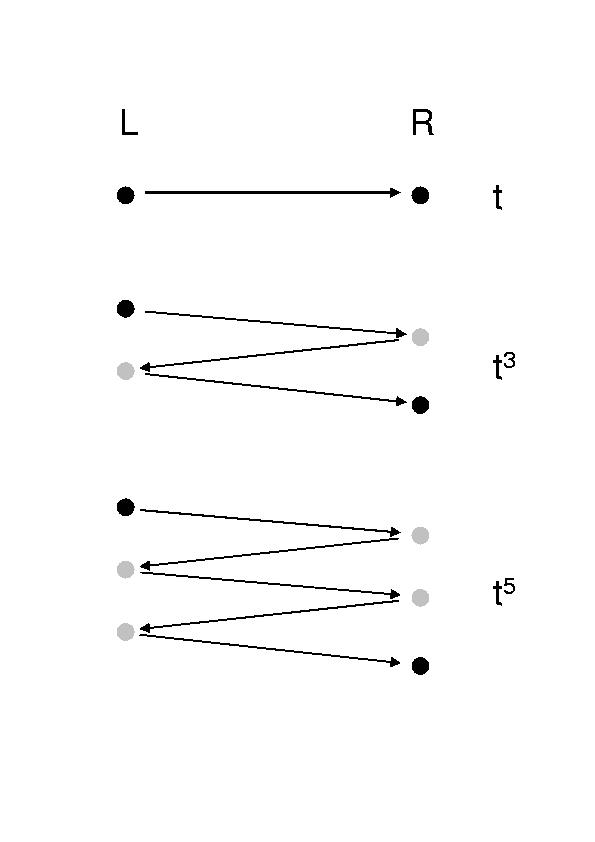
Figure 5: Transfer processes from left to right of different order.

Whereas $t$ is the single hopping amplitude, $T_{LR/RL}$ is a renormalized transfer amplitude. One may wonder why a model for transport could not have been set up adding amplitudes for transfer processes of all orders, as the interaction (18) seems to be introduced the way it is just in order to result in powers of $t$. However, $g^{r/a}(\omega)=\mp i$ deduced from the Schrödinger equation is decisive for the signs in (30) and (31). One may wonder that multiple reflections are not added as $t+t^{3}+t^{5}+\ldots=\frac{t}{1-t^{2}}$. Processes of different order (Fig.2) are not independent, but interfere. $T_{RL}$ is the transfer amplitude per single electron supplied on the left by the voltage source. But for every electron that goes over to the right in an $n$th order process ($n$ odd) with weight $t^{2}$ there is one that has hopped once more to the right and back ($n+2$ order process) and thus is not to be newly supplied, but to be again sent through the junction. The amplitude $t$ is renormalized by $1+t^{2}$ as denominator. However, such interpretations of quantum mechanical amplitudes are precarious, and the full conversion of $t$ to a transmission probability will be established later.

It is quite instructive to solve (27) in a slightly different way than done in (30). Firstly, for the four components in LR-space we have

$$T_{LL}=\phantom{\sigma_{RL}+}\sigma_{LR}g_{RR}T_{RL}\qquad T_{LR}=\sigma_{LR}+\sigma_{LR}g_{RR}T_{RR}$$

$$T_{RL}=\sigma_{RL}+\sigma_{RL}g_{LL}T_{LL}\qquad T_{RR}=\phantom{\sigma_{RL}+}\sigma_{RL}g_{LL}T_{LR}$$ (27a)

Inserting these into each other, for example, an equation for $T_{LR}$ alone is obtained:

$$T_{LR}=\sigma_{LR}+\sigma_{LR}g_{RR}\sigma_{RL}g_{LL}T_{LR}$$ (32)

This implicit equation is the basis for calulating the transfer Green’s function in more complicated cases than discussed here Cuequ ; my06 , like for example the superconducting junction. In our model, inserting $\sigma_{LR}=\sigma_{RL}=t$ and $g^{r/a}_{LL}(\omega)=g^{r/a}_{RR}(\omega)=\mp i$ into (32) immediately also leads to $T_{LR}^{r/a}(\omega)=\frac{t}{1+t^{2}}$.

Figure 6: Illustration of the Dyson equation for the transfer Green’s function.

More easily than the Dyson equation for the ordinary Green’s function $G$, the one for the transfer Green’s function $T$ is illustrated as is done for the LR-component in Fig.3. (Normally indices are read from right to left such that $T_{LR}$ is considered a transition from right to left, but it does not really matter whether they are interpreted the other way round as in Fig.3. The actual sequence of what is earlier or later in time will be discussed when calculating the current in the next section.) Fig.3 demonstrates the implicitness of the Dyson equation: Any transition from left to right is either a single transfer or an electron hopping to the right and back followed by any process beginning on the left and ending on the right, no matter what happens in between. This last part by definition is the sane as the other side of the equation, namely $T_{LR}$.

III.5 Calculating the current

From the Heisenberg picture of quantum mechanics we know that the time derivative of a not explicitly time-dependent operator $A$ is given by the commutator with the Hamiltonian CoTan_2 :

$$\frac{d}{d\tau}A=\frac{i}{\hbar}[H,A]$$ (33)

The operator of interest here is the projector on either side of the junction

$$\rho_{L}=\frac{|\Psi^{0}_{L}><\Psi^{0}_{L}|}{|\Psi^{0}_{L}|^{2}}\widehat{=}\begin{pmatrix}1&0\cr 0&0\cr\end{pmatrix}\quad{\rm or}\quad\rho_{R}=\frac{|\Psi^{0}_{R}><\Psi^{0}_{R}|}{|\Psi^{0}_{R}|^{2}}\widehat{=}\begin{pmatrix}0&0\cr 0&1\cr\end{pmatrix}$$ (34)

As explained earlier, with the junction coupling left and right together, the solution $\begin{pmatrix}\Psi_{L}\cr\Psi_{R}\cr\end{pmatrix}$ is not limited to one side, however, the projectors take out the respective part:

$$\begin{pmatrix}1&0\cr 0&0\cr\end{pmatrix}\begin{pmatrix}\Psi_{L}\cr\Psi_{R}\cr\end{pmatrix}=\begin{pmatrix}\Psi_{L}\cr 0\cr\end{pmatrix}\quad{\rm and}\quad\begin{pmatrix}0&0\cr 0&1\cr\end{pmatrix}\begin{pmatrix}\Psi_{L}\cr\Psi_{R}\cr\end{pmatrix}=\begin{pmatrix}0\cr\Psi_{R}\cr\end{pmatrix}$$ (34a)

$\rho_{L}$ and $\rho_{R}$ are proportional to the amount of charge on the left and on the right side. Their time derivatives have equal absolute values, but opposite sign and represent the current.

$$I=-e<\frac{d\rho_{L}}{d\tau}>=e<\frac{d\rho_{R}}{d\tau}>$$ (35)

($<\;|$ and $|\;>$ are used for bra- and ket-states. Here $<\;>$ means the expectation value, of course.) $e$ is the charge of an electron and the sign of $I$ can be defined arbitrarily. We choose to do the calculation with $\rho_{L}$ and evaluate the commutator with the Hamiltonian:

$$[H,\rho_{L}]=\left[\begin{pmatrix}H_{LL}&H_{LR}\cr H_{RL}&H_{RR}\cr\end{pmatrix},\begin{pmatrix}1&0\cr 0&0\cr\end{pmatrix}\right]=\underbrace{\begin{pmatrix}0&-H_{LR}\cr H_{RL}&0\cr\end{pmatrix}}_{\sigma_{c}}$$ (36)

Putting together (33) and (35) we obviously need the expectation value of the operator $[H,\rho_{L}]$. $[H,\rho_{L}]$ shall be called $\sigma_{c}$. Even if (33) stems from the Heisenberg picture, it is written in such a way, that the right hand side is to be evaluated in the Schrödinger system with time dependent states, and we shall here change to the interaction picture Mahan for the calculation. With ^† standing for complex conjugation as well as transposition from column to line vector, the value of ${\displaystyle\frac{d\rho_{L}}{dt}}$ in state $\begin{pmatrix}\Psi_{L}\cr\Psi_{R}\cr\end{pmatrix}$ at time $\tau$ is given by

$$\begin{pmatrix}\Psi_{L}(\tau)\cr\Psi_{R}(\tau)\end{pmatrix}^{\dagger}\;\frac{i}{\hbar}\;\begin{pmatrix}0&-H_{LR}(\tau)\cr H_{RL}(\tau)&0\end{pmatrix}\;\begin{pmatrix}\Psi_{L}(\tau)\cr\Psi_{R}(\tau)\end{pmatrix}=$$

$$<\Psi^{0}(\tau_{0})|\widetilde{T}\;\exp(\frac{1}{\hbar}\int_{\tau_{0}}^{\tau}i\;\sigma_{\mathcal{H}}(\tau^{\prime})\;d\tau^{\prime})\;i[H,\rho_{L}]_{\mathcal{H}}\;\widehat{T}\;\exp(\frac{1}{\hbar}\int_{\tau_{0}}^{\tau}(-i)\;\sigma_{\mathcal{H}}(\tau^{\prime})\;d\tau^{\prime})|\Psi^{0}(\tau_{0})>$$

$H_{LR}(\tau)$ and $H_{RL}(\tau)$ denote the time occurence of $\tau$ from (18) which has to be considered as still belonging to the Schrödinger picture in our case here. $\widehat{T}$ means time ordering Mahan and $\widetilde{T}$ anti-time ordering. $\Psi^{0}$ in the uncoupled system, of course, also stands for a two-vector with left and right component. Replacing $\begin{pmatrix}\Psi_{L}(\tau)\cr\Psi_{R}(\tau)\end{pmatrix}$ by $\Psi^{0}(\tau_{0})$ in (37) we took out both the coupling as well as the time dependence from the states. Accordingly the $\sigma_{\mathcal{H}}$ in the integrals, in contrast to the Schrödinger-picture $\sigma$ used in the preceding sections, in a Heisenberg way have to include the time dependence of the uncoupled states. $\sigma(\tau)$ could already be written as

$$\sigma(\tau)=\begin{pmatrix}0&H_{LR}(\tau)\cr H_{RL}(\tau)&0\cr\end{pmatrix}=\begin{pmatrix}e^{-i\omega_{L}\tau}&0\cr 0&e^{-i\omega_{R}\tau}\cr\end{pmatrix}\begin{pmatrix}0&W\cr W&0\cr\end{pmatrix}\begin{pmatrix}e^{i\omega_{L}\tau}&0\cr 0&e^{i\omega_{R}\tau}\cr\end{pmatrix}$$

or $\sigma(\tau)=|\Psi^{0}(\tau)>W<\Psi^{0}(\tau)|$ for short, where bra, ket and $W$ still mean the respective matrices. However, this decomposition might rather be confusing and will not be used, anyway. The translation to the interaction picture is the following:

$$\sigma_{\mathcal{H}} = \begin{pmatrix}e^{\frac{i}{\hbar}H_{LL}(\tau-\tau_{0})}&0\cr 0&e^{\frac{i}{\hbar}H_{RR}(\tau-\tau_{0})}\cr\end{pmatrix}\begin{pmatrix}0&H_{LR}(\tau)\cr H_{RL}(\tau)&0\cr\end{pmatrix}\begin{pmatrix}e^{-\frac{i}{\hbar}H_{LL}(\tau-\tau_{0})}&0\cr 0&e^{-\frac{i}{\hbar}H_{RR}(\tau-\tau_{0})}\cr\end{pmatrix}$$ (38)

$$= \begin{pmatrix}e^{-i\omega_{L}\tau_{0}}&0\cr 0&e^{-i\omega_{R}\tau_{0}}\cr\end{pmatrix}\begin{pmatrix}e^{i\omega_{L}\tau}&0\cr 0&e^{i\omega_{R}\tau}\cr\end{pmatrix}\;\begin{pmatrix}0&H_{LR}(\tau)\cr H_{RL}(\tau)&0\cr\end{pmatrix}\cdot$$

$$\qquad\qquad\qquad\qquad\qquad\qquad\begin{pmatrix}e^{-i\omega_{L}\tau}&0\cr 0&e^{-i\omega_{R}\tau}\cr\end{pmatrix}\begin{pmatrix}e^{i\omega_{L}\tau_{0}}&0\cr 0&e^{i\omega_{R}\tau_{0}}\cr\end{pmatrix}$$

or $\sigma_{\mathcal{H}}(\tau)=|\Psi^{0}(\tau_{0})><\Psi^{0}(\tau)|\;\sigma(\tau)\;|\Psi^{0}(\tau)><\Psi(\tau_{0})|$. The Heisenberg picture always refers the operator back to the undeveloped state at $\tau_{0}$.

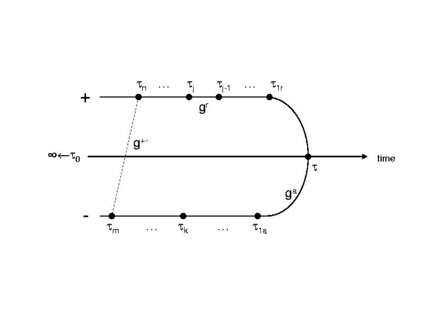
Figure 7: The Keldysh contour illustrating the development out of the uncoupled system’s states of the bra $<\Psi(\tau)|$ on the minus and the ket $|\Psi(\tau)>$ on the plus branch. This view picks out the single transition at time $\tau$ and visualizes the calculation of $<\Psi(\tau)|\sigma(\tau)|\Psi(\tau)>$. Each point on the contour represents an LR- or RL-transition described by $\sigma$, each line segment the development of the wave-function phase which is given $g$.

Analogously $\sigma_{c}$ will have to be extended by the time-dependence of the uncoupled states. The meaning of the time-integral over $\sigma_{\mathcal{H}}$ as an exponential is best explained by writing explicitly:

$$\widehat{T}\;\exp(\frac{1}{\hbar}\int_{\tau_{0}}^{\tau}(-i)\;\sigma_{\mathcal{H}}(\tau^{\prime})\;d\tau^{\prime})=\sum_{n}\frac{1}{\hbar}\int_{\tau_{2}}^{\tau}d\tau_{1}\ldots\frac{1}{\hbar}\int_{\tau_{j+1}}^{\tau_{j-1}}d\tau_{j}\ldots\frac{1}{\hbar}\int_{\tau_{0}}^{\tau_{n-1}}d\tau_{n}\cdot$$

$$(-i)\sigma_{\mathcal{H}}(\tau_{1})\ldots(-i)\sigma_{\mathcal{H}}(\tau_{j})\ldots(-i)\sigma_{\mathcal{H}}(\tau_{n})$$ (39)

where all arguments $\tau_{1},\ldots,\tau_{j},\ldots,\tau_{n}$ have to lie between $\tau_{0}$ and $\tau$ and all products from none to arbitrarily many factors $\sigma_{\mathcal{H}}$ have to be added. With time ordering, furthermore $\tau_{1}\geq\ldots\geq\tau_{j}\geq\ldots\geq\tau_{n}$ is imposed. Without $\widehat{T}$ the scheme for the exponential series $e^{x}=\sum_{n=0}^{\infty}\frac{x^{n}}{n!}$ in (39) would produce $\sum_{n}\frac{1}{n!}\;\frac{1}{\hbar}\int_{\tau_{0}}^{\tau}d\tau_{1}\ldots\frac{1}{\hbar}\int_{\tau_{0}}^{\tau}d\tau_{j}\ldots\frac{1}{\hbar}\int_{\tau_{0}}^{\tau}d\tau_{n}\ldots$ . But then for every fixed set $\{\tau_{1},\ldots,\tau_{j},\ldots,\tau_{n}\}$ there are $n!$ permutations for the time values to occur such that time ordering and restricting the arguments to mutually exclusive intervals as done in (39) cancels the factorial denominators. Writing out the anti-time ordered part in the same way as shown for the time-ordered part, the expression from (37) becomes

$${\bf<\Psi^{0}(\tau_{0})|}\quad\Psi^{0}(\tau_{0})>\frac{i}{\hbar}<\Psi^{0}(\tau_{m})|\sigma(\tau_{m})|\Psi^{0}(\tau_{m})><\Psi^{0}(\tau_{0})|\;\ldots$$

$$\ldots|\Psi^{0}(\tau_{0})>\frac{i}{\hbar}<\Psi^{0}(\tau_{k})|\sigma(\tau_{k})|\Psi^{0}(\tau_{k})><\Psi^{0}(\tau_{0})|\quad{\it\Psi^{0}(\tau_{0})>\frac{i}{\hbar}<\Psi^{0}(\tau_{k-1})|}$$

$${\it\sigma(\tau_{k-1})|}\ldots|\sigma(\tau_{1a})|\Psi^{0}(\tau_{1a})><\Psi^{0}(\tau_{0})|\quad{\bf\Psi^{0}(\tau_{0})>\frac{i}{\hbar}<\Psi^{0}(\tau)|\sigma_{c}(\tau)|}$$

$${\bf\Psi^{0}(\tau)><\Psi^{0}(\tau_{0})|}\quad\Psi^{0}(\tau_{0})>(\frac{-i}{\hbar})<\Psi^{0}(\tau_{1r})|\sigma(\tau_{1r})|\ldots$$

$${\it\ldots|\sigma(\tau_{j-1})|\Psi^{0}(\tau_{j-1})><\Psi^{0}(\tau_{0})}\quad|\Psi^{0}(\tau_{0})>(\frac{-i}{\hbar})<\Psi^{0}(\tau_{j})|\sigma(\tau_{j})|\Psi^{0}(\tau_{j})>$$

$$<\Psi^{0}(\tau_{0})|\ldots|\sigma(\tau_{n})|\Psi^{0}(\tau_{n})><\Psi^{0}(\tau_{0})\quad{\bf|\Psi^{0}(\tau_{0})>}$$ (37a)

where $\tau_{0}\leq\tau_{m}\leq\ldots\leq\tau_{k}\leq\ldots\tau_{1a}\leq\tau$, $\tau_{0}\leq\tau_{n}\leq\ldots\leq\tau_{j}\leq\ldots\leq\tau_{1r}\leq\tau$ and integration over all time arguments except $\tau$ and $\tau_{0}$ is understood. Like in (39) we mean the sum of all products with arbitrary many inner development factors like $\Psi^{0}$ of $\tau_{k}$ and $\Psi^{0}$ of $\tau_{j}$. Spaces and different font types are just used in (37a) to recognize sequential $\sigma_{\mathcal{H}}$-parts like (38). Inner development factors like $\Psi^{0}$ of $\tau_{k}$ and $\tau_{j}$ as well as $\Psi^{0}(\tau)$ and the inner $\Psi^{0}(\tau_{0})$ have to sum over space or the basis of states and therefore should be thought of as matrices as in (38). We have not yet decided which components outer bra and ket with ${\bf\Psi^{0}(\tau_{0})}$ will project out. All $<\Psi^{0}(\tau_{0})|\Psi^{0}(\tau_{0})>$ are the unit matrix and drop out ($\Psi^{0}$ being given by a non-normalizable $e$-function does not pose a problem here). Then $|\Psi^{0}(\tau_{k})>\frac{i}{\hbar}<\Psi^{0}(\tau_{k-1})|$ with $\tau_{k}\leq\tau_{k-1}$ is recognized as $g^{a}(\tau_{k},\tau_{k-1})$ and $|\Psi^{0}(\tau_{j-1})>\frac{(-i)}{\hbar}<\Psi^{0}(\tau_{j})|$ with $\tau_{j-1}\geq\tau_{j}$ as $g^{r}(\tau_{j-1},\tau_{j})$. These $g^{a/r}$ are 2x2 diagonal matrices. With (21) in (37a) the whole sequence from $|\Psi^{0}(\tau_{m})>$ to $<\Psi^{0}(\tau)|$ can be replaced by $G^{a}(\tau_{m},\tau)$ and the long part from $|\Psi^{0}(\tau)>$ up to $<\Psi^{0}(\tau_{n})|$ is just $G^{r}(\tau,\tau_{n})$. The complete operator between the outermost ${\bf<\Psi^{0}(\tau_{0})}|$ and ${\bf|\Psi^{0}(\tau_{0})>}$ in (37a) therefore becomes

$$|\Psi^{0}(\tau_{0})>\frac{i}{\hbar}<\Psi^{0}(\tau_{m})|\left[{\bf 1}\;\delta(\tau_{m}-\tau)+\sigma(\tau_{m})G^{a}(\tau_{m},\tau)\right]\sigma_{c}(\tau)$$

$$\left[{\bf 1}\;\delta(\tau_{n}-\tau)+G^{r}(\tau,\tau_{n})\sigma(\tau_{n})\right]|\Psi^{0}(\tau_{n})><\Psi^{0}(\tau_{0})|$$ (37b)

The ${\bf 1}$-contributions stem from the cases where there are no factors with $\Psi^{0}(\tau_{k})$ or $\Psi^{0}(\tau_{j})$. We regard the coupled system as having developed out of the uncoupled system, but we are looking for a stationary state. To achieve this, the coupling has to have been turned on infinitely long ago, thus we let $\tau_{0}\rightarrow-\infty$. The sequence of time arguments is usually represented on the so-called Keldysh contor (Fig.4). We still have to take the expectation value of (37) or (37a). This means summing over the basis of states for the outer ${\bf\Psi^{0}(\tau_{0})}$. The uncoupled basis consists of $\begin{pmatrix}1\cr 0\cr\end{pmatrix}$ and $\begin{pmatrix}0\cr 1\cr\end{pmatrix}$ for a state on the left and a state on the right for each frequency $\omega$. We shall discuss the occupation or emptiness of states shortly after having worked off some further more formal points. Summing over $\begin{pmatrix}1\cr 0\cr\end{pmatrix}$ and $\begin{pmatrix}0\cr 1\cr\end{pmatrix}$ for the outer ${\bf\Psi^{0}(\tau_{0})}$ will return the trace of the matrix $M$ given in (37b).

$$\begin{pmatrix}1\cr 0\cr\end{pmatrix}^{T}\underbrace{\begin{pmatrix}m_{11}&m_{12}\cr m_{21}&m_{22}\cr\end{pmatrix}}_{M}\begin{pmatrix}1\cr 0\cr\end{pmatrix}+\begin{pmatrix}0\cr 1\cr\end{pmatrix}^{T}\underbrace{\begin{pmatrix}m_{11}&m_{12}\cr m_{21}&m_{22}\cr\end{pmatrix}}_{M}\begin{pmatrix}0\cr 1\cr\end{pmatrix}={\rm Tr}\;M=m_{11}+m_{22}$$

Only being interested in the trace as a result, in a matrix multiplication the order of factor matrices can be changed cyclically. As in (37b) every bra and every ket as well as each operator part between the two $|$ is a matrix we can rotate factors to obtain

$$\sigma_{c}(\tau)\left[{\bf 1}\;\delta(\tau_{n}-\tau)+G^{r}(\tau,\tau_{n})\sigma(\tau_{n})\right]\quad|\Psi^{0}(\tau_{n})>\;\cdot$$

$$<\Psi^{0}(\tau_{0})|\Psi^{0}(\tau_{0})>\frac{i}{\hbar}<\Psi^{0}(\tau_{m})|\;\left[{\bf 1}\;\delta(\tau_{m}-\tau)+\sigma(\tau_{m})G^{a}(\tau_{m},\tau)\right]$$ (37c)

$<\Psi^{0}(\tau_{0})|\Psi^{0}(\tau_{0})>={\bf 1}$ again drops out. $|\Psi^{0}(\tau_{n})>\frac{i}{\hbar}<\Psi^{0}(\tau_{m})|$ is of the structure $g$, however, with no restriction as to which argument $\tau_{n}$ or $\tau_{m}$ is earlier or later in time. We define this new type of Green’s function as

$$g^{+-}(\tau,\tau^{\prime},\omega)=\frac{i}{\hbar}e^{-i\omega(\tau-\tau^{\prime})}=\begin{cases}-g^{r}(\tau,\tau^{\prime},\omega)\quad{\rm if}\;\tau>\tau^{\prime}\\ \phantom{-}g^{a}(\tau,\tau^{\prime},\omega)\quad{\rm if}\;\tau<\tau^{\prime}\end{cases}$$ (40)

(An eventually ill-defined single point $\tau=\tau^{\prime}$ is irrelevant for later integrations.) As the cases $\tau>\tau^{\prime}$ and $\tau<\tau^{\prime}$ are mutually exclusive the function can also be given by $g^{+-}(\tau,\tau^{\prime})=g^{a}(\tau,\tau^{\prime})-g^{r}(\tau,\tau^{\prime})$ (conclusions on $g^{+-}(\omega)$ from that are risky, to my opinion, though). We have thus deduced the current formula

$$I(\tau) = -e\;{\rm Tr}\;\{\;\sigma_{c}(\tau)\int_{-\infty}^{\tau}d\tau_{n}\int_{-\infty}^{\tau}d\tau_{m}\;\left[({\bf 1}\delta(\tau_{n}-\tau)+G^{r}(\tau,\tau_{n})\sigma(\tau_{n})\right]\;\cdot$$ (41)

$$\cdot\;g^{+-}(\tau_{n},\tau_{m})\;\left[{\bf 1}\delta(\tau_{m}-\tau)+\sigma(\tau_{m})G^{a}(\tau_{m},\tau)\right]\;\}$$

(like discussed in (20) it is rather irrelevant whether the upper integration limits are set as $\tau$ or $\infty$) or

$$I(\tau)=-e\;{\rm Tr}\;\left\{\sigma_{c}(\tau)\;G^{+-}(\tau,\tau)\right\}$$ (41a)

if $G^{+-}$ is defined as

$$G^{+-}(\tau,\tau^{\prime})=\int d\tau_{1}\int d\tau_{2}\; [{\bf 1}\delta(\tau_{1}-\tau)+G^{r}(\tau,\tau_{1})\sigma(\tau_{1})]\;g^{+-}(\tau_{1},\tau_{2})\cdot$$ (42)

$$[{\bf 1}\delta(\tau_{2}-\tau)+\sigma(\tau_{2})G^{a}(\tau_{2},\tau^{\prime})]$$

or

$$G^{+-}=({\bf 1}+G^{r}\sigma)\;g^{+-}\;({\bf 1}+\sigma G^{a})$$ (42a)

in short notation. The current only needs $G^{+-}$ of two identical time arguments. We shall need the Fourier representation of $g^{+-}(\omega)$, but none such for $G^{+-}$. Although in our simple model for the normal-conducting contact the current will come out the same for any $\tau$, $I(\tau)$ generally does depend on time (our expectation value is an ensemble, not a time average). For the superconducting case the ac parts Cuequ like the Josephson current are included in the expression (41), although one is mostly interested in the contribution in $I$ that is independent of $\tau$ and gives the dc part.

Using $g^{+-}(\tau_{n},\tau_{m})$ without a third argument $\omega$ in (41) we understood integration over frequency like in (16). But this point requires more care as it has not been taken into account so far whether states are occupied or empty at $\tau_{0}\rightarrow-\infty$. Writing out the trace from (41a) in LR-components reveals four contributions

$$-I/e = \sigma_{c,LR}\;(1+G^{r}_{RL}\sigma_{LR})\;g^{+-}_{RR}\;\sigma_{RL}G^{a}_{LL}$$ (43)

$$+ \sigma_{c,LR}\;G^{r}_{RR}\sigma_{RL}\;g^{+-}_{LL}\;(1+\sigma_{LR}G^{a}_{RL})$$

$$+ \sigma_{c,RL}\;G^{r}_{LL}\sigma_{LR}\;g^{+-}_{RR}\;(1+\sigma_{RL}G^{a}_{LR})$$

$$+ \sigma_{c,RL}\;(1+G^{r}_{LR}\sigma_{LR})\;g^{+-}_{LL}\;\sigma_{LR}G^{a}_{RR}$$

It is clear that in contrast to the other appearing $\sigma$, in $\sigma_{c}$ from (36) there is an additional relativ minus sign between the LR- and the RL-component. Obviously the net current is the difference between the current from left to right and the current from right to left. In the first - as well as the second - term in (43) a transition from R to L at $\tau$, the time argument of $\sigma_{c}$, is picked out to be counted for the current (see also Fig.4). With $g^{+-}$ at R, the charge carrier is supplied from a state originally located on the right. It is an electron if the energy lies below the right-side Fermi level. Until $\tau$ the state has evolved to again be on the right. The originally left behind empty state at the same energy below the Fermi level must have evolved to be on the left at $\tau$ such that by the R$\rightarrow$L transfer the electron can go into it (Fig.5a). Or you might say that the plus and the minus branch of the Keldysh contor represent two possible parts in the evolution of an original wave function $\Psi^{0}_{R}$, between which there is a non-vanishing matrix element of the operator $\sigma_{c}=[H,\rho_{L}]$. However, still regarding the first line of (43), there is the further possibility that an empty state from above the Fermi level on the right evolves to be at R at $\tau$ again, but its left-behind complement (a negative charge) has evolved to be at L. $\sigma_{LR}(\tau)$ in this case means the transition of an empty state or positively charged particle from right to left (Fig.5b). Although one does not usually introduce the concept of holes with transport in normal conducting metals, it makes sense here to call unoccupied states simply ”holes”. In this way the model already includes the dual nature of charge carriers needed for the superconducting case. In the normal conducting case states do not change in nature (electron or hole) or energy during their evolution (little zigzags are drawn in Fig.5 only to make the multiple hoppings visible). At the superconducting junction, Andreev reflection can be interpreted as changing an electron into a hole or vice versa and mirroring its energy at the Fermi level my06 (see Fig.9 in section 6). To have a charge carrier at a certain energy level at time $\tau$ to make a certain transition, it is important that there was one at the corresponding energy in the original uncoupled system. The coupling may have changed the distribution compared to the occupation in uncoupled bulk reservoirs. And the applied voltage imposes a non-equilibrium situation, anyway. For the evolution of a state from the right as shown in Fig.5 it does not matter whether the state at the respective energy on the left is occupied or empty. If, for example the regarded energy lies below the Fermi levels both left and right, there will be two states evolving as an electron on the plus and a hole on the minus branch of the Keldysh contor, one having originated at R and the other at L. These original, uncoupled and independent states are our basis, especially for calculating an expectation value as trace. They do not interfere. Terms with $g^{+-}_{RR}$ and $g^{+-}_{LL}$ are simply added in (43). Schemes analogous to Fig.5 could be drawn for the terms from the last three lines of (43) as well. The conclusion of the whole argumentation of how to let the original Fermi occupation function for the reservoirs left and right enter the current calculation is that $g^{+-}_{LL}$ has to change sign at the left Fermi energy and $g^{+-}_{RR}$ at the right Fermi energy. Let us note $g^{+-}$ like $g^{r}$ and $g^{a}$ for any bulk reservoir with Fermi level at $\omega=0$. We shall keep $g^{+-}$ corresponding to $g^{r}$ and $g^{a}$ as in (40) for occupied electron states below the Fermi level and change the sign for empty states above it.

$$g^{+-}(\tau,\tau^{\prime})=\frac{\mathcal{D}}{h}\int d\omega\;g^{+-}(\omega)\;e^{-i\omega(\tau-\tau^{\prime})}\;{\rm with}\;g^{+-}(\omega)=\begin{cases}\phantom{-}i\;{\rm for}\;\omega<0\\ -i\;{\rm for}\;\omega>0\end{cases}$$ (44)

Although it might be practical to use (19), (23), (44), (18) and (36) in (41) to quite directly produce an expression that calculates the current finally as an integral over frequency and in our simple model can even be analytically evaluated, in parallel to Cuequ we shall use the transfer Green’s functions here. The current is best translated into an expression of the transfer functions from the form already resolved into LR-components (43). Furthermore eliminate $\sigma_{c}$ through $\sigma_{c,LR}=-\sigma_{LR}$ and $\sigma_{c,RL}=\sigma_{RL}$. L- and R-indices follow logically from (26), for example $G_{LL}\sigma_{LR}=g_{LL}T_{LR}$.

$$I/e = \sigma_{LR}\;(1+g^{r}_{RR}T^{r}_{RR})\;g^{+-}_{RR}\;T^{a}_{RL}g^{a}_{LL}$$ (43a)

$$+ \sigma_{LR}\;g^{r}_{RR}T^{r}_{RL}\;g^{+-}_{LL}\;(1+T^{a}_{LL}g^{a}_{LL})$$

$$- \sigma_{RL}\;g^{r}_{LL}T^{r}_{LR}\;g^{+-}_{RR}\;(1+T^{a}_{RR}g^{a}_{RR})$$

$$- \sigma_{RL}\;(1+g^{r}_{LL}T^{r}_{LL})\;g^{+-}_{LL}\;T^{a}_{LR}g^{a}_{RR}$$

As quantities here are no longer matrices, but simply functions of time or frequency, the leading $\sigma_{LR}$ and $\sigma_{RL}$ in the second and third line of (43a) can be moved to the ends of the products. From (41) we remember that their argument is $\tau$, the same as the second argument of the last factor to the right. Then using relations from (27a) and complementary forms the current formula simplifies to

$$I/e = T^{r}_{LR}g^{+-}_{RR}T^{a}_{RL}g^{a}_{LL}\;+\;g^{r}_{RR}T^{r}_{RL}g^{+-}_{LL}T^{a}_{LR}$$ (43b)

$$- g^{r}_{LL}T^{r}_{LR}g^{+-}_{RR}T^{a}_{RL}\;-\;T^{r}_{RL}g^{+-}_{LL}T^{a}_{LR}g^{a}_{RR}$$

The terms with the factors 1 from the brackets have elegantly been made to vanish. Now we use the Fourier representations for all functions in (43b). As all terms follow the same scheme, the second is treated in an exemplary way here (all integrals run from $-\infty$ to $+\infty$):

$$\int d\tau_{1}\;d\tau_{2}\;d\tau_{3}\;d\omega_{1}\;d\omega\;d\omega_{2}\;d\omega_{3}\;\frac{\mathcal{D}}{h}g^{r}_{RR}(\omega_{1})e^{-i\omega_{1}\tau}e^{i\omega_{1}\tau_{1}}\frac{\hbar}{2\pi\mathcal{D}}T^{r}_{RL}(\omega_{2})$$

$$e^{-i(\omega_{2}+eV/\hbar)\tau_{1}}e^{i\omega_{2}\tau_{2}}\;\frac{\mathcal{D}}{h}g^{+-}_{LL}(\omega)e^{-i\omega\tau_{2}}e^{i\omega\tau_{3}}\frac{\hbar}{2\pi\mathcal{D}}T^{a}_{LR}(\omega_{3})e^{-i\omega_{3}\tau_{3}}e^{i(\omega_{3}+eV/\hbar)\tau}$$

Doing the $\tau_{1}$,$\tau_{2}$- and $\tau_{3}$-integrals gives $(2\pi)^{3}\delta(\omega_{1}-\omega_{2}-eV/\hbar)\delta(\omega_{2}-\omega)\delta(\omega-\omega_{3})$. Then even the exponentials with $\tau$ cancel and the term simplifies to

$$\frac{1}{2\pi}\int d\omega\;g^{r}_{RR}(\omega+eV/\hbar)\;T^{r}_{RL}(\omega)\;g^{+-}_{LL}(\omega)\;T^{a}_{LR}(\omega)$$

In our case (31) tells us that $T^{r/a}_{LR/RL}(\omega)$ are all identical and real, $g^{r}_{LL/RR}(\omega)=-i$ is the complex conjugate of $g^{a}_{LL/RR}(\omega)=i$ and $-g^{+-}_{LL/RR}$ is the complex conjugate of $g^{+-}_{LL/RR}$ of the same $\omega$ as $g^{+-}(\omega)$ is purely imaginary, too. Thus the last two terms in (43b) are the complex conjugates of the first two and thus twice the real part of these first two can be taken for $I/e$. In the superconducting version of the model, where $T$ and $g$ actually are $\omega$-dependent, complex conjugate relations my06 also exist between $T$s as well as $g$s, and the current formula can be reduced in the same way. Just to note the quite general formula Cuequ in short form:

$$I/e=2\;{\rm Re}\;\left\{T^{r}_{LR}g^{+-}_{RR}T^{a}_{RL}g^{a}_{LL}+g^{r}_{RR}T^{r}_{RL}g^{+-}_{LL}T^{a}_{LR}\right\}$$ (45)

For the integrand from the second term in our model we get

$$g^{r}_{RR}(\omega+eV/\hbar)T^{r}_{RL}(\omega)g^{+-}_{LL}(\omega)T^{a}_{LR}(\omega)=(-i)\frac{t}{1+t^{2}}(\mp i)\frac{t}{1+t^{2}}=\mp\frac{t^{2}}{(1+t^{2})^{2}}$$

where the signs refer to $\omega$ greater or less than zero and come out reversed for the first term with $g^{+-}_{RR}$, because there is $g^{a}$ instead of $g^{r}$. Care has to be taken with the reference point for $\omega$ in both terms. This may easily be overlooked in the normal conducting case here in contrast to the superconducting case where $T$ indeed is $\omega$-dependent and like $G$ as a function of only one argument always referred to the same Fermi level (the left, for example). If we call the argument of $g^{+-}_{LL}$ from the second term $\omega$, the one for $g^{+-}_{RR}$ in the first term is $\omega+eV/\hbar$. On an $\omega_{(L)}$-axis, the second term changes sign at zero, however, the first jumps at $-eV/\hbar$ (Fig.6). A shift of the integration parameter cannot be made independently for both terms. Thus, for the normal conducting model here

$$I/e=2\;{\rm Re}\;\frac{1}{2\pi}\int d\omega\;\{\;T^{r}_{LR}(\omega)g^{+-}_{RR}(\omega+\frac{eV}{\hbar})T^{a}_{RL}(\omega)g^{a}_{LL}(\omega)$$

$$+\;g^{r}_{RR}(\omega+\frac{eV}{\hbar})T^{r}_{RL}(\omega)g^{+-}_{LL}(\omega)T^{a}_{LR}(\omega)\;\}$$ (45a)

In principle the convention is needed, that the $T$-argument always refers to the left side, but for $g$ general formula like (44) for a single bulk with Fermi level at zero frequency are applied. A more involved situation where choosing integration intervals consistently for all contributing current terms is crucial can be found in my06 .

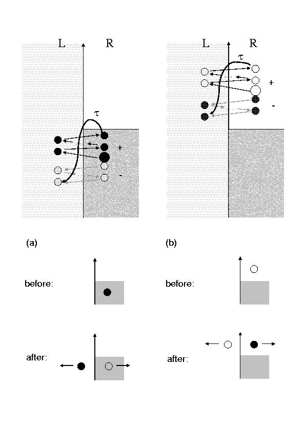
Figure 8: (a) Evolution of an electron state from R such that at $\tau$ the charge is transferred to the left. (b) Evolution of an unoccupied state above the Fermi level from R such that at $\tau$ it gets filled by a charge from the left or the hole state shifts to the left. The lower pictures sketch the effect of the original uncoupled state for the current. Sending electrons from the right to the left will be compensated by electrons sent from left to right. But with levels as in Fig.1c for holes sent from right to left there will be a range between the two Fermi levels where there are no counterbalancing holes going the other way. (For the left, electrons going to the right are not outweighed in this range.)

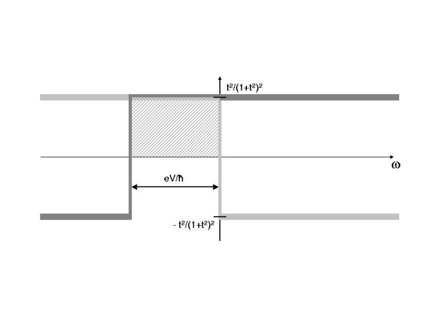
Figure 9: The two terms under the integral from equation (45). They cancel except on an interval of length $eV/\hbar$.

From Fig.6 it is easily seen that that the integral is twice the constant $\frac{t^{2}}{(1+t^{2})^{2}}$ integrated over an interval of length $eV/\hbar$, and outside that interval contributions cancel. With the other factor 2 from twice the real part and the prefactor $1/2\pi$ the result for the current finally is

$$I/e=2\cdot\frac{1}{2\pi}\cdot 2\cdot\frac{t^{2}}{(1+t^{2})^{2}}\cdot\frac{eV}{\hbar}\quad\quad\Longleftrightarrow$$

$$\frac{V}{I}=\frac{h}{e^{2}}\left(\frac{4t^{2}}{(1+t^{2})^{2}}\right)^{-1}\qquad\Longleftrightarrow\qquad\frac{I}{V}=\frac{e^{2}}{h}\frac{4t^{2}}{(1+t^{2})^{2}}$$ (46)

The factor $\theta=4t^{2}/(1+t^{2})^{2}$ is the conductance in units of the quantum conductance or its inverse the resistance in units of the quantum resistance Cuequ . (The conductance of a channel doubles if two spin states are allowed. Then $h/2e^{2}=13k\Omega$ should be taken as resistance unit.) $\theta$ is the transmission probability of the conductance channel through the junction we regarded. The result that in the normal-conducting case the current is proportional to the voltage is not at all surprising, of course. The non-trivial result is the conversion of the quantum mechanical transmission amplitude $t$ to the measurable transmission probability $\theta$. $\theta=0$ if $t=0$. And a totally open channel with $t=1$ has transmission probability $\theta=1$.

It may seem a contradiction on the one hand calculating the current from a changing amount of charge on one side and on the other hand saying that missing charges are replaced and superfluous ones led away by the voltage source. A slightly different viewpoint may help to get convinced that the calculated quantity is indeed the current in the stationary, but non-equilibrium system. The crucial point was putting on to evaluate $d\rho_{L}/dt$ in state $\Psi(t)$. Without further ado we could not tell whether this state of the coupled system was occupied or not. The Schrödinger equation (5) set up the left and right material properties as well as the coupling across the junction, however, did not take any account of the effect of the voltage source. Without need to specify real locations for the division, just principally view our structure as consisting of a junction region and leads. The $\Psi(t)$ defined through (5) describes states in the junction region. But think of them as offered by the system and following their time development whether occupied or not. The leads are always occupied exactly up to their Fermi levels. Electrons freshly supplied by the voltage source need not be in phase with present ones. A random phase is most easily modelled by assuming the left lead wave function at any time $\begin{pmatrix}1\cr 0\cr\end{pmatrix}$ without a phase in contrast to the assumed $\begin{pmatrix}\exp(-i\omega_{L}\tau)\cr 0\cr\end{pmatrix}$ for the left side of the junction region. Which states to which extent actually get occupied in the left side of the junction region, that is $\rho_{L}(t)$, is determined by the overlap of $\Psi(t)$ with the phaseless left lead wave function $\begin{pmatrix}1\cr 0\cr\end{pmatrix}$, which we recognize as $\Psi_{L}^{0}(-\infty)$. $\rho_{L}=|<\begin{pmatrix}1\cr 0\cr\end{pmatrix}|\begin{pmatrix}\Psi_{L}(t)\cr 0\cr\end{pmatrix}>|^{2}$. The current then is the change in time of $\rho_{L}$ due to charge flow through the junction, that is processes inside the junction region only, corresponding to what our Hamiltonian was set up for. A similar line of thought with state overlaps can be applied to the passing of charges out of the junction region into the (right) lead; it may be helpful to view this as putting empty states or holes into the junction region, though. Of course, only the L-part of $\Psi(t)$ can overlap with $\begin{pmatrix}1\cr 0\cr\end{pmatrix}$. $\begin{pmatrix}\Psi_{L}(t)\cr 0\cr\end{pmatrix}$ can thus be replaced by $\Psi(t)$ in our new expression for $\rho_{L}$. Recalling the operator definition (34) the time derivative of $\rho_{L}$

$$\frac{d}{dt}\;\rho_{L}=\frac{d}{dt}\;|<\begin{pmatrix}1\cr 0\cr\end{pmatrix}|\Psi(t)>|^{2}=\frac{d}{dt}\left\{<\Psi(t)|\begin{pmatrix}1\cr 0\cr\end{pmatrix}><\begin{pmatrix}1\cr 0\cr\end{pmatrix}|\Psi(t)>\right\}$$

is identical to the ansatz made by putting together (33) and (34) in (37).

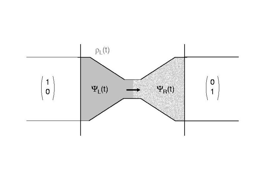
Figure 10: Hypothetical division of the structure into the actual junction region and bulk leads.

III.6 Comment on the two-level system

At first glance the problem posed by the Schrödinger equations without and with coupling, (1) and (5), especially if we regard a single energy level on each side with corresponding $\omega_{L}$ and $\omega_{R}$ as in Fig.1c, looks like the two-level system known from quantum mechanics textbooks CoTan . By the coupling the two energy levels are shifted. The new eigenstates lie further apart from one another. If the system is initiated in one of the uncoupled states, it will oscillate harmonically between the two levels, and both both the period of the oscillation as well as the maximum transition probability to the other state depend on the energy difference of the original states.

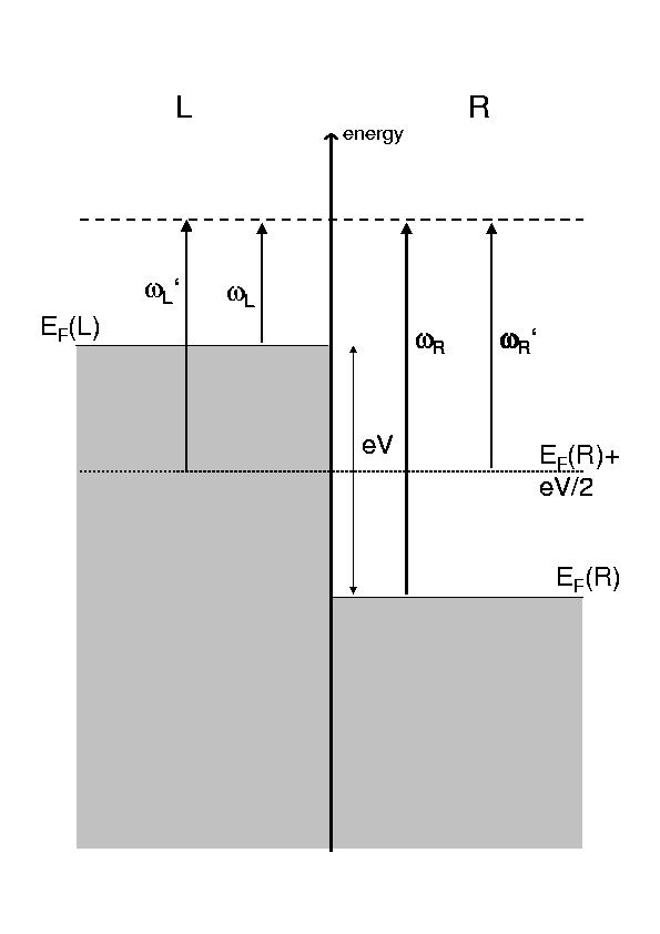
Figure 11: Attempt to adjust energy levels from left and right to same reference.

Even if the time dependence of the interaction (18) can be got rid of by changing to the interaction picture, it makes no sense to numbly calculate eigenvalues and eigenvectors of a Hamiltonian $\begin{pmatrix}\hbar\omega_{L}&W\cr W&\hbar\omega_{R}\cr\end{pmatrix}$. It is not clear from which reference levels such eigenenergies $E_{\pm}$ should be counted as zero levels are different for $\omega_{L}$ and $\omega_{R}$. If one tries to refer the left and right energies already of the uncoupled system to the same reference level, $E_{F}(R)+\frac{eV}{2}$ for example (Fig.8), $\Psi^{0}_{L}$ (and $\Psi^{0}_{R}$) cannot be taken as eigenstates any more, because from $i\hbar\partial_{\tau}e^{-i\omega_{L}\tau}=\hbar\omega_{L}e^{-i\omega_{L}\tau}$ with $\omega_{L}=\omega_{L}^{\prime}+\frac{eV}{2}$ it does not follow that $i\hbar\partial_{\tau}e^{-i(\omega_{L}^{\prime}+eV/2)\tau}$ equals $\hbar\omega_{L}^{\prime}e^{-i(\omega_{L}^{\prime}+eV/2)\tau}$. The standard treatment of the two-level system is not applicable to the non-equilibrium situation.

III.7 Superconducting junction

Despite having been the simplest example to introduce the Green’s functions scheme, applying the formalism to the normal conducting junction to get out that the current is proportional to the applied voltage was breaking a butterfly on the wheel. Although repeatedly mentioned, fully developing the extension to the superconducting case is beyond the scope of this presentation. But the resulting current-voltage characteristics shall be shown as a plea for the usefulness of the method. A different approach based on matching wave functions AveBar leads to identical results, though.

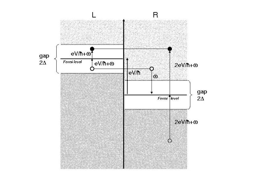
Figure 12: Illustration of Andreev reflection as mirroring at the Fermi levels for electron-hole conversion and vice versa. For either side the incoming and reflected levels can lie inside or outside the gap. Only the beginning and end of a complete multiple-reflection process have to be in the electron or hole reservoir below or above the gap, respectively.

Some formula shall be listed, because they are not necessarily written out in complete analogy to the presentation here in Cuequ and other literature. Working in the quasiparticle picture, in the superconducting case each entry in LR-space of a Green’s or transfer function expands into another 2x2 matrix in Nambu space over electrons and holes. There is ketterson_2 :

$$g^{r/a}_{LL/RR}(\omega)=\begin{pmatrix}g^{ee}&g^{eh}\cr g^{he}&g^{hh}\cr\end{pmatrix}^{r/a}_{LL/RR}(\omega)=\frac{1}{\sqrt{(\Delta/\hbar)^{2}-(\omega\pm i\eta)^{2}}}\begin{pmatrix}-\omega\mp i\eta&\Delta/\hbar\cr-\Delta/\hbar&\omega\pm i\eta\cr\end{pmatrix}$$ (47)

$g$ is the same for LL and RR. Different signs refer to the retarded and advanced function. $\Delta$ is half the gap of the superconductor. The small imaginary part $\eta$ is added to get the correct root besides slightly smoothening singularities. $g(\tau,\tau^{\prime})=\mathcal{D}/h\;\int d\omega\;g(\omega)\;e^{-i\omega\tau}\;e^{i\omega\tau^{\prime}}$ still holds.

$$\sigma_{LR/RL}=\begin{pmatrix}\sigma^{ee}&0\cr 0&\sigma^{hh}\end{pmatrix}_{LR/RL}=\frac{\hbar}{\mathcal{D}}\;\begin{pmatrix}t\;e^{\pm ieV\tau/\hbar}&0\cr 0&-t\;e^{\mp ieV\tau/\hbar}\end{pmatrix}$$ (48)

Here signs refer to the LR- and RL-direction, respectively. Remark the reversed signs for holes in the exponential compared to electrons. There is no electron-hole conversion during a single hopping. The $eh$- and $he$-elements of $g$ introduce so-called Andreev reflection. (Cooper-pair tunneling Urbina is not included.) $T$ is a full matrix in $eh$-space and has to be set up as

$$\frac{\mathcal{D}}{\hbar}\;T(\tau,\tau^{\prime})=\frac{1}{2\pi}\sum_{n}\int d\omega\;T_{n}(\omega)\;e^{-i\omega\tau}\;e^{ineV\tau/\hbar}\;e^{i\omega\tau^{\prime}}$$ (49)

We skipped the distinction of reference $\omega_{J/K}$ as in (25), because in practice only one type, e.g. $T_{LR}$, has to be calculated, as then $T_{RL}$ follows from complex conjugation. $n$ runs over all integers. A Dyson equation like (32) leads to a recursion which connects $T_{n}$ to $T_{n-2}$ and $T_{n+2}$. It can be solved by reasonably truncating the $n$-range. Then, just also summing over $n$, the established current formula (45) can be used.

Expressions like (32) have to sum over all possible combinations of $e$- and $h$-indices. For example:

$$T^{ee}_{LR}=\sigma_{LR}^{ee} + \sigma_{LR}^{ee}g^{ee}_{RR}\sigma_{RL}^{ee}g^{ee}_{LL}T^{ee}_{LR}+\sigma_{LR}^{ee}g^{eh}_{RR}\sigma_{RL}^{hh}g^{he}_{LL}T^{ee}_{LR}$$ (50)

$$+ \sigma_{LR}^{ee}g^{ee}_{RR}\sigma_{RL}^{ee}g^{eh}_{LL}T^{he}_{LR}+\sigma_{LR}^{ee}g^{eh}_{RR}\sigma_{RL}^{hh}g^{hh}_{LL}T^{he}_{LR}$$

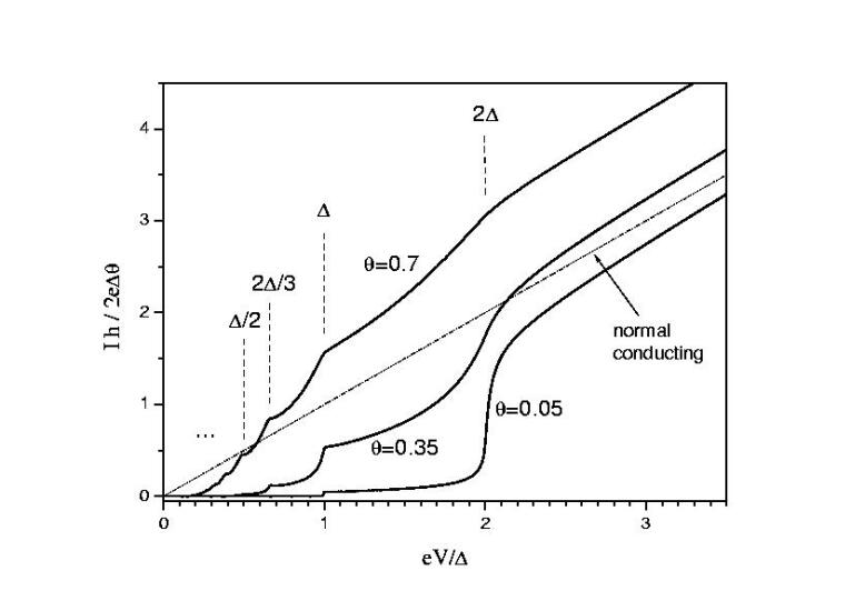
Figure 13: Calculated current-voltage curves for transport channels of three different transmissions (normalized to $\theta$) [reproduced after Cuequ ]. The normal conducting $IV$ is added for comparison (keep $\Delta$ just for units).

To point out the Andreev reflection in the model, we look at a term $g\sigma g\sigma g$ with alternating $e$- and $h$-indices from the development (21). Such a sequence will also be contained as parts in higher-order terms from (21) or (24). Contracting inner time arguments results in

$$\int d\tau_{1}\;d\tau_{2}\;g^{(h)e}_{RR}(\tau,\tau_{1})\;\sigma^{ee}_{RL}(\tau_{1})\;g^{eh}_{LL}(\tau_{1},\tau_{2})\;\sigma^{hh}_{LR}(\tau_{2})\;g^{h(e)}_{RR}(\tau_{2},\tau^{\prime})$$ (51)

$$= \int d\tau_{1}\;d\tau_{2}\;d\omega_{2}\;d\omega_{1}\;d\omega\;\frac{\mathcal{D}}{h}g^{(h)e}_{RR}(\omega_{2})e^{-i\omega_{2}\tau}e^{i\omega_{2}\tau_{1}}\;\frac{\hbar}{\mathcal{D}}te^{-ieV\tau_{1}/\hbar}\;\cdot$$

$$\phantom{++}\frac{\mathcal{D}}{h}g^{eh}_{LL}(\omega_{1})e^{-i\omega_{1}\tau_{1}}e^{i\omega_{1}\tau_{2}}\;\frac{\hbar}{\mathcal{D}}(-t)e^{-ieV\tau_{2}/\hbar}\;\frac{\mathcal{D}}{h}g^{h(e)}_{RR}(\omega)e^{-i\omega\tau_{2}}e^{i\omega\tau^{\prime}}$$

$$= (-t^{2})\;\frac{\mathcal{D}}{h}\int d\omega\;d\omega_{1}\;d\omega_{2}\;\delta(\omega_{2}-\frac{eV}{\hbar}-\omega_{1})\;\delta(\omega_{1}-\frac{eV}{\hbar}-\omega)\;\cdot$$

$$\phantom{+++++}g^{(h)e}_{RR}(\omega_{2})\;g^{eh}_{LL}(\omega_{1})\;g^{h(e)}_{RR}(\omega)\;e^{-i\omega_{2}\tau}\;e^{i\omega\tau^{\prime}}$$

$$= -t^{2}\;\frac{\mathcal{D}}{h}\int d\omega\;g^{(h)e}_{RR}(\omega+2\frac{eV}{\hbar})\;g^{eh}_{LL}(\omega+\frac{eV}{\hbar})\;g^{h(e)}_{RR}(\omega)\;e^{-i(\omega+2eV/\hbar)\tau}\;e^{i\omega\tau^{\prime}}$$

because the $\tau_{1}$ and $\tau_{2}$-integration give $4\pi^{2}\delta(\omega_{2}-eV/\hbar-\omega_{1})\delta(\omega_{1}-eV/\hbar-\omega)$. In Fig.9 for holes the energy axis has to be reversed as compared to electrons. Therefore the initial $\omega$ is negative. For the argument here, it does not matter if the beginning factor in (51) is $g^{he}_{RR}$ or $g^{ee}_{RR}$. If it were $h$, then the Andreev reflection marked by the dashed arrow would follow. The last index of the last $g_{RR}$ could also be $h$ instead of $e$. Whereas in the normal conducting case in multiple reflections the charge carrying particle always came back to the same energy with regard to the Fermi level when coming back to the same side of the junction (Fig.1), in (51) the frequency argument of the first $g_{RR}$ is shifted by twice the applied voltage equivalent with respect to the second $g_{RR}$ (Fig.9). Such shifts enable transport even when the gaps of the left and right side are still overlapping, that is for voltages below $2\Delta/e$ (Fig.10). In the $IV$-curves steps towards lower voltages at fractions of $2\Delta$ are associated to ever higher-order Andreev reflections. Of course, these current contributions become the more prominent the greater the channel transmission. Besides the step heights and positions the curvature on each step is an important signature. The model agrees excellently with experimental results Sche97 . The interference of transport processes of different order is correctly taken into account. Simpler models Bratus that add up tranfer probabilities proportional to $\theta^{order}$ cannot reproduce these characteristics and are only valid for low transmissions $\theta<<1$.

IV Conclusions and Outlook for section III

It has been explained on a quite basic level how quantum transport between two reservoirs in a stationary non-equilibrium state can be modelled. The purpose was to present a Green’s functions technique for handling coupling in the context of a field of current research interest, namely transport through point contacts. Although besides the general formalism (also see section I) requiring the development of quite some more subject specific mathematical framework such as the transfer Green’s functions, the transport through a contact with arbitrary transmission is a suitable example to illustrate the inclusion of interaction up to all orders in the implicit Dyson equations. Calculations have been carried through in every detail for the normal-conducting single junction. Basic formula and results have been given for the superconducting junction. The decomposition into transport channels (eigenmodes) of a point contact can be inferred from its superconducting transport characteristics which can be taken like a PIN-code Sche97 . The presented Green’s functions formalism has a great potential for extension. Systems of two more or less coherently linked junctions can be modelled my06 . Models for transport through molecules Heurich ; Roland ; Wohltat or atomic chains Mertig so far mainly rely on ab initio calculations of the density of states. Time dependent density functional theory for non-equilibrium situations is also developed Kurth .

- (1) Ohtaka K 1993 Green’s Functions in: Encyclopedia of Applied Physics (VCH Publishers) p 341
- (2) Doniach S and Sondheimer E H 1978 Green’s Functions for Solid State Physicists (Frontiers in Physics, Lecture Note Series, second printing, W.A.Benjamin Inc.)
- (3) Koonin S E 1986 Computational Physics (TheBenjamin/Cummings) chapter 3.3
- (4) Friedrich A 1998 Anfangs-, Rand- und Eigenwertprobleme in Technik und Physik (expert verlag) chapters 1.3.5 and 3.3.5
- (5) Chicanne C, David T, Quidant R, Weeber J C, Lacroute Y, Bourillot E and Dereux A 2002 Phys.Rev.Lett. 88 097402
- (6) Scheer E, Agrait N, Cuevas J C, Levy-Yeyati A, Ludoph B, Martin-Rodero A, Rubio-Bollinger G, vanRuitenbeek J and Urbina C 1998 Nature 394 154
- (7) Cuevas J C, Martin-Rodero A and Levy Yeyati A 1996 Phys.Rev. B 54 7366
- (8) Girard C, Dereux A, Martin O J F and Devel M 1994 Phys.Rev. B 50 14467; Girard C, Dereux A, Martin O J F and Devel M 1995 Phys.Rev. B 52 2889
- (9) Schröter U 2003 Eur.Phys.J. B 33 297
- (10) Jackson J D 1999 Classical Electrodynamics, 3rd ed. (Wiley) chapter 1.10 references for section II:
- (11) Greffet J J and Carminati R 1997 Progress in Surface Science 56 p.133-237
- (12) Dereux A, Girard C and Weeber J C 2000 J.Chem.Phys. 112 7775
- (13) Girard C, Dereux A, Martin O J F and Devel M 1995 Phys.Rev. B 52 2889
- (14) Kottmann J P, Martin O J F, Smith D R and Schultz S 2001 Chem.Phys.Lett. 341 1
- (15) Gerard D, Wenger J, Bonod N, Popov E, Rigneault H, Mahdavi F, Blair S, Dintinger J and Ebbesen T W 2008 Phys.Rev. E 77 045413
- (16) Jackson J D 1999 Classical Electrodynamics, 3rd ed. (Wiley) chapters 2 and 3
- (17) Dereux A, Devaux E, Weeber J C, Goudonnet J P and Girard C 2001 Journal of Microscopy 202 320
- (18) Devaux E, Dereux A, Bourillot E, Weeber J C, Lacroute Y, Goudonnet J P 2000 Phys.Rev.B 62 10504
- (19) Chicanne C, David T, Quidant R, Weeber J C, Lacroute Y, Bourillot E and Dereux A 2002 Phys.Rev.Lett. 88 097402
- (20) Gotschy W, Vonmetz K, Leitner A and Aussenegg F R 1996 Opt.Lett. 21 1099
- (21) Weeber J C, Girard C, Krenn J R, Dereux A and Goudonnet J P 1999 J.Appl.Phys. 86 2576
- (22) Krenn J R, Wolf R, Leitner A and Aussenegg F R 1997 Opt.Comm. 137 46
- (23) Perney N M B, Garcia de Abajo F J, Baumberg J J, Tang A, Netti M Cm Charlton M D B and Zoorob M E 2007 Phys.Rev. E 76 035426
- (24) Krenn J R, Dereux A, Weeber J C, Bourillot E, Lacroute Y, Goudonnet J P, Schider G, Gotschy W, Leitner A, Aussenegg F R and Girard C 1999 Phys.Rev.Lett. 82 2590
- (25) Weeber J C, Dereux A, Girard C, Colas des Francs G, Krenn J R and Goudonnet J P 2000 Phys.Rev. E 62 7381; Girard C, Dereux A and Joachim C 1999 Phys.Rev. E 59 6097
- (26) Paulus M and Martin O J F 2001 J.Opt.Soc.Am. A 18 854
- (27) Quidant R, Leveque G, Weeber J C, Dereux A, Girard C and Weiner J 2004 Europhys.Lett. 66 785
- (28) thio T, Pellerin K M, Linke R A, Lezec H J and Ebbesen T W 2001 Opt.Lett. 26 1972
- (29) Girard C, Dujardin E, Li M and Mann S 2006 Phys.Rev.Lett. 97 100801
- (30) Schröter U 2003 Eur.Phys.J. B 33 297
- (31) Colas des Francs G, Girard C, Weeber J C, Chicanne C, David T, Dereux A and Peyrade D 2001 Phys.Rev.Lett. 86 4950
- (32) Chew W 1990 Waves and fields in inhomogeneous media (vanNostrand Reinhold, New York) chapter 7
- (33) Dereux A 1991 thesis, Facultes Universitaires Notre-Dame de la Paix, Namur
- (34) Jackson J D 1999 Classical Electrodynamics, 3rd ed. (Wiley) chapter 9.2
- (35) Kopitzki k 1989 Einführung in die Festkörperphysik, 2nd ed. (Teubner) chapter 4.1
- (36) Jackson J D 1999 Classical Electrodynamics, 3rd ed. (Wiley) chapter 4.4
- (37) Callaway J 1976 Quantum Theory of the Solid State (Academic Press) chapter 5.2.3
- (38) Jackson J D 1999 Classical Electrodynamics, 3rd ed. (Wiley) chapter 6.9
- (39) Girard C, David T, Chicanne C, Mary A, Colas des Francs G, Bourillot E, Weeber J C and Dereux A 2004 Europhys.Lett. 68 797
- (40) Alonso M and Finn E J 1980 Fundamental University Physics I, Mechanics and Thermodynamics, 2nd ed. (Addison-Wesley) chapter 12.13
- (41) Crommie M F, Lutz C P and Eigler D M 1993 Science 262 218; Manoharan H C, Lutz C P and Eigler D M 2000 Nature 403 512
- (42) Hecht T, Pohl D W, Heinzelmann H and Novotny L 1995 Ultramicroscopy 61 99
- (43) Girard C, Weeber J C, Dereux A, Martin O J F and Goudonnet J P 1997 Phys.Rev.B 55 16487
- (44) Martin O J F and Piller N B 1998 Phys.Rev. E 58 3909
- (45) Paulus M, Gay-Balmaz P and Martin O J F 2000 Phys.Rev.E 62 5797; Paulus M and Martin O J F 2001 Phys.Rev.E 63 066615
- (46) Dereux A private communication references for section III:
- (47) Agrait N, Levy Yeyati A, van Ruitenbek J M 2003 Phys.Rep. 377 p.81-279
- (48) Rubio G, Agrait N and Vieira S 1996 Phys.Rev.Lett. 76 2302
- (49) Heersche H B, Lientschnig G, O’Neill K, van der Zant H and Zandbergen H W 2007 Appl.Phys.Lett. 91 072107
- (50) Krans J M, Muller C J, Yanson I K, Govaert T C M, Hesper R, van Ruitenbek J M 1993 Phys.Rev. B 48 14721
- (51) van Wees B J, van Houten H, Beenakker C W J, Williamson J G, Kouwenhoven L P, van der Marel D and Foxon C T 1988 Phys.Rev.Lett. 60 848; Beenakker C W J and van Houten H 1991 Solid State Physics 44 1
- (52) Büttiker M, Imry Y, Landauer R and Pinhas S 1985 Phys.Rev. B 31 6207
- (53) Scheer E, Joyez P, Esteve D, Urbina C and Devoret M H 1997 Phys.Rev.Lett. 78 3535; Scheer E, Agrait N, Cuevas J C, Levy-Yeyati A, Ludoph B, Martin-Rodero A, Rubio-Bollinger G, vanRuitenbeek J and Urbina C 1998 Nature 394 154
- (54) Grabert H and Devoret M H (ed.) 1992 Single Charge Tunneling, Coulomb Blockade Phenomena in Nanostructures (Nato ASI Series, Plenum Press) chapter 1.1
- (55) Häfner M, Konrad P, Pauly F, Cuevas J C and Scheer E 2004 Phys.Rev. B 70 241404
- (56) Levy-Yeyati A, Cuevas J C and Martin-Rodero A 2005 Phys.Rev.Lett 95 056804
- (57) Ketterson J B and Song S N 1999 Superconductivity (Cambridge University Press) chapter 47.3
- (58) Cuevas J C, Martin-Rodero A and Levy Yeyati A 1996 Phys.Rev. B 54 7366
- (59) Schröter U and Scheer E 2006 Phys.Rev. B 74 245301; Schröter U and Scheer E 2007 Phys.Rev. B 76 205104
- (60) Cohen-Tannoudji C, Diu B and Laloë F 1999 Quantenmechanik, 2nd ed. (deGruyter, Berlin) chapter 3.12
- (61) Mahan G D 2000 Many-Particle Physics, 3rd ed. (Kluwer Academic/Plenum Publishers) chapter 2.1
- (62) Cohen-Tannoudji C, Diu B and Laloë F 1999 Quantenmechanik, 2nd ed. (deGruyter, Berlin) chapter 4.3
- (63) Averin D and Bardas A 1995 Phys.Rev.Lett. 75 1831
- (64) Ketterson J B and Song S N 1999 Superconductivity (Cambridge University Press) chapter 55
- (65) Goffman MF, Cron R, Levy Yeyati A, Joyez P, Devoret M H, Esteve D and Urbina C 2000 Phys.Rev.Lett. 85 170; Bylander J, Duty T, Johansson G and Delsing P 2007 Phys.Rev. B 76 020506
- (66) Bratus E N, Shumeiko V S and Wnedin G 1995 Phys.Rev.Lett. 74 2110
- (67) Heurich J, Cuevas J C, Wenzel W and Schön G 2002 Phys.Rev.Lett. 88 256803; Reichert J, Ochs R, Beckmann D, Weber H B, Mayor M and von Löhneysen H 2002 Phys.Rev.Lett. 88 176804
- (68) Roland C, Meunier V, Larade B and Guo H 2002 Phys.Rev. B 66 035332
- (69) Wohlthat S, Pauly F, Viljas J K, Cuevas J C and Schön G 2007 Phys.Rev. B 76 075413
- (70) Bagrets A, Papanikolaou N and Mertig I 2006 Phys.rev. B 045428
- (71) Kurth S, Stefanucci G, Almbladh C O, Rubio A and Gross E K U 2005 Phys. Rev. B 72 035308; Stefannucci G, Kurth S and Gross E K U 2006 cond-mat/0607333