Dynamics of the Solar Magnetic Network.
II. Heating the magnetized chromosphere

Abstract

We consider recent observations of the chromospheric network, and argue that the bright network grains observed in the Ca II H & K lines are heated by an as yet unidentified quasi-steady process. We propose that the heating is caused by dissipation of short-period magnetoacoustic waves in magnetic flux tubes (periods less than 100 s). Magnetohydrodynamic (MHD) models of such waves are presented. We consider wave generation in the network due to two separate processes: (a) by transverse motions at the base of the flux tube; and (b) by the absorption of acoustic waves generated in the ambient medium. We find that the former mechanism leads to an efficient heating of the chromosphere by slow magnetoacoustic waves propagating along magnetic field lines. This heating is produced by shock waves with a horizontal size of a few hundred kilometers. In contrast, acoustic waves excited in the ambient medium are converted into transverse fast modes that travel rapidly through the flux tube and do not form shocks, unless the acoustic sources are located within 100 km from the tube axis. We conclude that the magnetic network may be heated by magnetoacoustic waves that are generated in or near the flux tubes.

1 Introduction

In the chromosphere on the quiet Sun it is useful to distinguish between the magnetic network on the boundary of supergranulation cells (Simon & Leighton, 1964), where strong magnetic fields are organized in mainly vertical flux tubes, and internetwork regions in the cell interiors, where magnetic fields are weaker and dynamically less important.

The canonical picture of the magnetic network is that it consists of vertical magnetic fields clumped into elements or flux tubes that are located in intergranular lanes, have magnetic field strengths in the kilogauss range, and have diameters of the order of 100 km or less at their footpoints in the photosphere (e.g., Gaizauskas, 1985; Zwaan, 1987). These magnetic elements can be identified with bright points seen in images taken in the G-band (4305 Å). High resolution observations show that these flux elements are in a highly dynamical state due to buffeting by convective flows on granular and supergranular scales (e.g., Muller et al., 1994; Berger et al., 1995, 1998; Berger & Title, 1996; Nisenson et al., 2003). With the availability of new ground-based telescopes at excellent sites and sophisticated image reconstruction techniques it is now possible to examine magnetic elements with an improved resolution of about 0.17 arcsec and investigate their structure and dynamics in unprecedented detail (e.g., Berger et al., 2004; Rouppe van der Voort et al., 2005; Langangen et al., 2007). High-quality observations of photospheric magnetic fields are now also being obtained with the Solar Optical Telescope (SOT) on Hinode (e.g., Lites et al., 2007, 2008; Rezaei et al., 2007). Magneto-convection models have been developed to understand the three-dimensional (3-D) structure and evolution of the magnetic field and its interactions with convective flows (e.g., Vögler et al., 2005; Schaffenberger et al., 2006).

The chromospheric network is most clearly seen in filter images taken in the Ca II H & K lines (e.g., Gaizauskas, 1985; Rutten, 2007) and in the Ca II IR triplet (Cauzzi et al., 2007). In H or K line images the network shows up as a collection of “coarse mottles” or “network grains” that stand out against the darker background. The network grains are continuously bright with intensities that vary slowly in time, in contrast to the “fine mottles” or “cell grains” which are located in the cell interiors and are much more dynamic (e.g., Rutten & Uitenbroek, 1991). In space-time diagrams derived from Ca II H spectra (e.g., Fig. 3 in Cram & Damé, 1983), the network grains show up as long bright streaks, indicating lifetimes of at least 10 min. The Ca II H line profiles of network grains are more symmetrical than those from the cell interior, and both the ${\rm H}_{2V}$ and ${\rm H}_{2R}$ features generally appear bright (Lites et al., 1993; Sheminova et al., 2005). Superposed on this constant brightness are low-frequency oscillations with periods of 5 to 20 min. (Lites et al., 1993; Kontogiannis et al., 2006; Tritschler et al., 2007); these oscillations have also been observed at UV wavelengths (e.g., Bloomfield et al., 2006).

The physical processes that produce the enhanced emission in Ca II network grains have not been identified. Are they heated by wave dissipation, and if so, what is the nature of these waves? In this paper we focus on the question why the emission from network grains is so constant in time. We discuss the observations, and investigate whether waves with periods $P<100$ s can provide the heating of the grains.

Hasan et al. (2005, hereafter Paper I) considered (magneto)acoustic waves generated at the interface of magnetic flux tubes and the outside medium. They suggested that such waves are generated as a result of interactions of flux tubes with turbulent downflows in intergranular lanes just below the photosphere. Intergranular lanes have widths of order 100 km, and downflow velocities of several km s^-1, so velocity fluctuations $\delta v\sim 1$ km s^-1 may be expected. Such fluctuations would produce transverse displacements of the flux tubes within the intergranular lanes. Assuming random displacements with amplitude $\delta x\sim 10$ km, the typical time scale is $\tau\sim 10$ s. Such perturbations would produce transverse waves with period $P\sim 2\tau$ that travel upward along the flux tube, as well as pressure fluctuations on either side of the tube (Paper I). Therefore, from a theoretical perspective it is reasonable to expect the existence of short-period magnetoacoustic waves in flux tubes ($P\sim 20$ s).

In this paper we present models of wave propagation in magnetic flux tubes that are relevant to the heating of the network grains. Specifically, we present two-dimensional (2-D) magnetohydrodynamic (MHD) simulations of the interactions of short-period waves with magnetic flux sheets (we shall use the terminology flux sheet and flux tube interchangeably). Although such simulations do not include the Alfvén mode, they provide a possible model for the waves involved in heating the Ca II grains. This work is a continuation of the study in Paper I.

The plan of the paper is as follow. In §2 we review recent observations of the chromospheric network, and we argue that the network grains are heated by an as yet unidentified quasi-steady process. We propose that the heating is due to short-period waves ($P<100$ s), although there is little evidence for such waves at present. In §3 we describe a 2-D MHD model for the propagation of short-period waves in magnetic flux tubes. In §4 we present simulation results for waves generated inside a flux tube; interaction of waves on different flux tubes are also considered. In §5 we consider the interaction of a flux tube with waves generated by acoustic sources located outside the flux tube. The final §6 discusses and summarizes the main results of this investigation.

2 Observations of Ca II Network Grains

Figure 1 shows an example of a network element observed with the Dutch Open Telescope (DOT, Rutten et al., 2005). The different panels show filtergrams in the blue continuum, G band, Ca II H line center, and Ca II H off band. The DOT uses a filter with a 1.4 Å FWHM passband centered on Ca II H (3968 Å), which covers the two chromospheric emission peaks on either side of line center, but also includes parts of the inner wings of the line, which originate in the upper photosphere. An examination of the G-band image confirms the picture of a network patch consisting of multiple flux elements. A comparison with the Ca II line center image shows that the excess chromospheric emission is localized directly above the photospheric flux tubes, although the bright features seen in Ca II are more diffuse than those seen in the G-band. Time sequences of such images show that the chromospheric network is continually bright (e.g., Tritschler et al., 2007).

Sheminova et al. (2005) combined high-resolution Ca II H and K spectra of network elements with flux tube modeling, and found that the excess brightness in the wings of the H and K lines compared with the quiet photosphere is primarily due to low density, not to mechanical heating. However, both the ${\rm H}_{2V}$ and ${\rm H}_{2R}$ emission features appear bright, indicating sustained non-thermal heating at heights where these features are formed (also see Lites et al., 1993). The Ca II profiles from network elements are nearly symmetric, indicating that the heating does not involve strong shocks such as those found in internetwork regions (Carlsson & Stein, 1997).

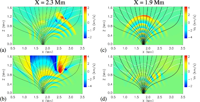
Figure 8: Field-aligned ($V_{s}$) and transverse ($V_{n}$) components of the velocity at $t=140$ s for a localized acoustic source at $z=0$, $x=2.3$ Mm (panels [a] and [b]) and $x=1.9$ Mm (panels [c] and [d]). The black curves denote the magnetic field lines, and the white curves are contours of constant $\beta$ ($\beta=0.1$, 0.3 and 1.0). The velocity in the region corresponding to $B<20$ G is not shown.

Rutten (2006, 2007) presented reviews and a synthesis of recent high-resolution observations of the solar chromosphere. In the Ca II H & K lines, the network shows up as a collection of “Ca II bright points” or “grains”. He also identifies an exciting new phenomenon called “straws” that extend radially outward from network bright points (see Figure 8 in Rutten, 2007). These straws are very thin, occur in “hedge rows”, and are very short-lived (10-20 s). They appear to be closely related to the so-called type-II spicules recently identified in limb observations with Hinode/SOT (De Pontieu et al., 2007b). The type-II spicules are much more dynamic than ordinary (type-I) spicules, are very thin (width $\sim 100$ km), have lifetimes of 10-150 s, and seem to be rapidly heated to transition region temperatures, sending material though the chromosphere at speeds of 50-150 $\rm km~{}s^{-1}$. De Pontieu and collaborators suggest that type-II spicules may be due to small-scale reconnection events in the chromosphere. De Pontieu et al. (2007c) show that the spicules exhibit transverse motions with velocities of 10 to 25 $\rm km~{}s^{-1}$, which provides evidence for the existence of Alfvén waves in the chromosphere.

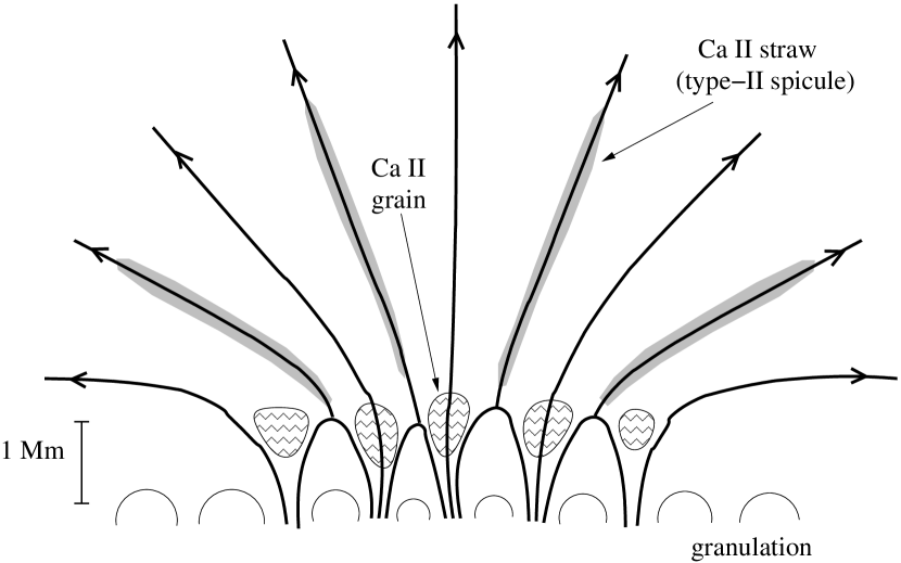
Figure 2: Schematic diagram showing the structure of a magnetic network element on the quiet Sun. The thin half-circles at the bottom of the figure represent the granulation flow field, and the thick curves represent magnetic field lines of flux tubes that are rooted in the intergranular lanes. The Ca II bright grains are thought to be located inside the flux tubes at heights of about 1 Mm above the base of the photosphere. We suggest that the Ca II “straws” (Rutten, 2006) may be located at the boundaries between the flux tubes.

In Ca II observations of network elements on the solar disk, the thin straws are superposed on the bright grains. According to Rutten (2006): “The network bright points are less sharp than and differ in morphology from G-band bright points … bright stalks emanate a few arcseconds from them at this resolution … diffuse Ca II H core brightness spreads as far or farther” (see his Fig. 2). Rutten conjectures that the bright Ca II network grains are nothing but a collection of straws seen nearly end-on. However, this is difficult to reconcile with the observed steadiness of the emission from network elements at high spatial resolution. Since the straws are very short-lived and dynamic, a superposition of many such features would be required to produce apparantly steady emission, but such high density of straws is not consistent with the limb observations by De Pontieu et al. (2007b, c). Also, if the plasma in the straws is hot ($T\sim 10^{5}$ K), as Rutten (2006) suggests, one would expect the straws to produce pure emission profiles, but the observed Ca II H & K line profiles from network elements are nearly symmetric and always show a central reversal (see Fig. 5 in Sheminova et al., 2005). Therefore, we suggest that most of the emission from Ca II grains is due to some quasi-steady heating process at heights of 500 km to 1500 km inside the magnetic flux tubes, and is not associated with spicule-like activity at larger heights.

Our interpretation of the Ca II observations is summarized in Figure 2, where we show a vertical cross section of a magnetic network element consisting of several discrete flux tubes. We suggest that the Ca II network grains are located inside the magnetic flux tubes, and give rise to the bulk of the Ca II emission from the network element. The grains are thought to be located at heights between 500 km and 1500 km above the photosphere where the flux tubes are no longer “thin” compared to the pressure scale height (about 200 km), but are still well separated from each other. The Ca II straws (type-II spicules) have widths of order 100 km, and are located at larger heights (several Mm) where the widths of the flux tubes are much larger than 100 km. Therefore, we suggest the straws are not directly associated with the network grains in the low chromosphere. In Figure 2 we assumed that the straws (type-II spicules) are located at the interfaces between the flux tubes, as suggested by van Ballegooijen & Nisenson (1998).

Observations have shown “magnetic shadows” surrounding network elements where the oscillations in the 2 - 4 minute range are suppressed (Judge et al., 2001; Krijger et al., 2001; Vecchio et al., 2007). These shadows have been attributed to the effects of highly structured magnetic fields on wave propagation and mode conversion in the chromosphere (McIntosh & Judge, 2001). Network elements on the quiet Sun exhibit oscillations with periods in the range 5 - 20 min. (e.g., Lites et al., 1993; Bloomfield et al., 2006). These long-period oscillations are thought to be driven by the interaction of vertical or inclined magnetic flux tubes with global p-modes and convective flows in the photosphere, producing magnetoacoustic shocks that drive spicules and spicule-like features at larger heights in the chromosphere (De Pontieu et al., 2004, 2005; Hansteen et al., 2006; Heggland, De Pontieu & Hansteen, 2007; Rouppe van der Voort et al., 2007). Jefferies et al. (2006) argued that inclined magnetic fields at the boundaries of supergranules may act as portals through which low-frequency magnetoacoustic waves can propagate into the solar chromosphere (also see McIntosh & Jefferies, 2006).

It seems unlikely that long-period waves are also responsible for the heating of the Ca II network grains in the low chromosphere. Simulations of shock waves with periods $P\sim 200$ s in a plane-parallel, non-magnetic atmosphere have shown that such waves produce large asymmetries in the Ca II H line profiles, and strong variations in the integrated emission. If the grains were heated by such long-period waves, they should exhibit similar strong intensity variations. This is not observed, so the long-period waves observed in network elements cannot be the main source of heating for the Ca II grains.

Network grains could possibly be heated by dissipation of waves with shorter periods ($P<100$ s). Ground-based observations of high-frequency waves in small network elements are affected by seeing, so it is possible that waves with periods $P<100$ s do exist in network elements but are simply not observable from the ground. This hypothesis could be tested using Ca II H images from Hinode/SOT (Tsuneta et al., 2007; Kosugi et al., 2007), keeping in mind of course that the passband of the Ca II H filter also includes a significant photospheric contribution. Alternatively, network grains could be heated by dissipation of Alfvén waves. There is evidence for Alfvén waves in spicules (De Pontieu et al., 2007c), and if these waves originate below the photosphere they must travel through the heights where the Ca II network grains are located. At present there is no direct observational evidence for Alfvén waves in flux elements in the photosphere, nor at heights where the Ca II H line is formed. Also, simulations of such waves in flux tubes would require 3-D MHD models. Therefore, in the present paper we focus on magnetoacoustic waves, which can be simulated with 2-D MHD models.

3 Models for Magnetoacoustic Waves in Network Elements

3.1 Background

Earlier work on wave dynamics idealized the network in terms of thin flux tubes (e.g., Roberts & Webb, 1978), and treated wave propagation in terms of the well known transverse (kink) and longitudinal (sausage) modes (e.g., Spruit, 1981). Several investigations have focused on the generation and propagation of transverse and longitudinal wave modes and their dissipation in the chromosphere (e.g., Zhugzhda et al., 1995; Fawzy et al., 2002; Ulmschneider, 2003, and references therein). Hasan & Kalkofen (1999) examined the excitation of transverse and longitudinal waves in magnetic flux tubes by the impact of fast granules on flux tubes, as observed by Muller & Roudier (1992) and Muller et al. (1994), and following the investigation by Choudhuri et al. (1993), who studied the generation of kink waves by footpoint motion of flux tubes. The observational signature of the modelled process was highly intermittent in radiation emerging in the H and K lines, contrary to observations. By adding waves that were generated by high-frequency motion due to the turbulence of the medium surrounding flux tubes the energy injection into the gas inside a flux tube became less intermittent, and the time variation of the emergent radiation was in better agreement with the more steady observed intensity from the magnetic network (Hasan et al., 2000).

The above studies on the magnetic network make use of two important idealizations: they assume that the magnetic flux tubes are thin, an approximation that becomes questionable at about the height of formation of the emission peaks in the cores of the H and K lines; and they neglect the interaction of neighboring flux tubes. Some progress on the first issue was made by Rosenthal et al. (2002) and Bogdan et al. (2003), who studied wave propagation in a 2-D stratified atmosphere, assuming the magnetic field can be approximated by a potential field. They examined the propagation of waves that are excited from spatially localized sources in the photosphere, and found that there is strong mode coupling between fast and slow waves at the so-called magnetic canopy, which they identify as the surface where the magnetic and gas pressures are comparable. However, potential-field models do not provide an accurate description of the boundary layers between the flux tubes and the ambient medium, where electric currents flow perpendicular to the magnetic field. In Paper I we considered more realistic, magnetostatic equilibrium models in which flux sheets are embedded in a field-free medium. In such models the boundary layer between the flux tube and its surroundings is sharper than in a potential field model (the width of the boundary layer is spatially resolved, see §3.2). This strongly affects the propagation and reflection of waves at the boundary (Hasan et al., 2006). Also, the shape of the $\beta=1$ surface in a magnetostatic model can be quite different from that in a potential-field model.

In the present paper we further develop the model for MHD wave propagation presented in Paper I. The initial configuration consists of one or more flux sheets in magnetostatic equilibrium with a relatively sharp interface between the flux sheets and the surrounding gas, unlike previous studies in which a potential field is considered (e.g., Rosenthal et al., 2002; Bogdan et al., 2003). The present work goes beyond Paper I in three important aspects: firstly, it seeks to understand how the dynamics of a flux tube is affected when the magnetic field in the wave excitation region is not that strong, so that the $\beta=1$ surface (approximately the level where the sound and Alfvén speeds become equal) lies above the base on the tube axis. Observations have revealed that the magnetic field strengths in the network are not uniformly kilogauss but have a range of values that go from strong to moderate (e.g., Berger et al., 2004). For moderate field strengths, wave generation occurs in a region where the field is essentially weak. Such waves undergo transformation higher up in the atmosphere. Secondly, we allow for the presence of multiple flux tubes in a network patch. We investigate the dynamical coupling between neighboring flux tubes and identify the regions responsible for the enhanced emission in the magnetic chromosphere. Finally, we examine the hypothesis that the magnetic network can be heated by acoustic waves from the ambient medium. More details of the model are provided in the next subsections.

Hansteen et al. (2006) and De Pontieu et al. (2007a) performed advanced 2-D numerical simulations that span the entire solar atmosphere from the convection zone to the lower corona. These simulations describe the evolution of a radiative MHD plasma: the model includes the effects of non-gray, non-LTE radiative energy transport in the photosphere and chromosphere, as well as field-aligned thermal conduction and optically thin radiative losses in the transition region and corona. They find that MHD waves generated by convective flows and oscillations in the lower photosphere naturally leak upward into the magnetized chromosphere, where they form shocks that can drive spicule-like jets. These models include more physics than the one presented here, but we believe our approach is adequate for the task of simulating short-period magnetoacoustic waves.

3.2 Equilibrium Model

In the solar photosphere the magnetic flux tubes are spatially separated from each other, and are rooted in intergranular lanes. In Paper I we considered a model for the structure of a magnetic network element as a collection of unipolar flux tubes (also see Cranmer & van Ballegooijen, 2005; Cranmer et al., 2007). We presented a two-dimensional model with an array of identical flux tubes separated by 1200 km. The flux tubes expand with height and merge into a monolithic structure at a height of about 500 km. In the present paper we present modified versions of this model. The method for constructing such models is summarized below.

The equilibrium magnetic field ${\bf B}(x,z)$ is a function of horizontal coordinate $x$ and height $z$ above the level where the optical depth $\tau_{5000}=1$ in the photosphere. The field is assumed to be periodic in the $x$ coordinate; the period length $L_{x}$ equals the distance between the flux tubes. The tubes are assumed to symmetric with respect to their vertical axes, therefore in the equilibrium model only one half of one flux tube needs to be considered. For the model presented in §4.1, the size of the computational domain is given by $\Delta x=L_{x}/2=1800$ km and $\Delta z=2950$ km, and we use a grid spacing of 5 km. At the lower boundary ($z=0$), the flux tube has a nearly Gaussian profile with $1/e$-width of 65 km. The 2-D structure of the flux tube is determined by solving the force balance equation:

$$-\nabla p+\rho{\bf g}+\frac{1}{4\pi}(\nabla\times{\bf B})\times{\bf B}=0,$$ (1)

where ${\bf g}=-g\hat{\bf z}$ is the gravitational acceleration, $p(x,z)$ is the gas pressure, and $\rho(x,z)$ is the density. The third term describes the Lorentz force due to electric currents at the boundary between the flux tube and its surroundings. The magnetic field is written in terms of a flux function $A(x,z)$ such that $B_{x}=-\partial A/\partial z$ and $B_{z}=\partial A/\partial x$. The gas pressure is given by

$$p(x,z)=p_{int}(z)\left[1+\beta_{0}^{-1}F(A)\right],$$ (2)

where $p_{int}(z)$ is the internal gas pressure as function of height along the axis of the flux tube ($A=0$); $\beta_{0}$ is the ratio of gas- and magnetic pressures at the base (on axis); and $F(A)$ is a function describing the variation of gas pressure across field lines ($F=0$ on axis and $F=1$ in the ambient medium). A similar expression holds for the gas density. The functions $p_{int}(z)$ and $F(A)$ are described in Paper I, except that in the present paper we use $\beta_{0}=2$. Equation (1) is solved for $A(x,z)$ using an energy minimization technique (see Paper I). Table 1 lists the basic parameters of the equilibrium model on the tube axis and in the ambient medium at the base ($z=0$) and at height $z=1500$ km in the chromosphere.

To construct the initial conditions for the MHD dynamical model, the equilibrium model is mirrored horizontally to create a single flux tube, and then further replicated to produce an array of flux tubes. Only the lower part of the equilibrium model is used ($z<1600$ km). Therefore, the magnetic field at the top of the MHD model is not vertical.

3.3 Dynamical Model and Boundary Conditions

We consider wave generation in the configuration described in the previous section by perturbing the lower boundary and solving the 2-D MHD equations in conservation form for an inviscid adiabatic fluid. These consist of the usual continuity, momentum, entropy (without sources) and magnetic induction equations (see Steiner et al., 1994). The unknown variables are the density, momentum, entropy per unit mass and the magnetic field. We assume that the plasma consists of fully ionized hydrogen with a mean molecular weight of 1.297. The temperature is computed from the specific entropy and the pressure is found using the ideal gas law.

The MHD equations are solved following the numerical procedure given by Steiner et al. (1994) and also described in Hasan et al. (2005). Briefly, the equations are discretized on a 2-D mesh and solved using a finite difference method based on the flux-corrected transport (FCT) scheme of Oran & Boris (1987). The time integration is explicit and has second-order accuracy in the time step. Small time steps are required to satisfy the Courant condition in the upper part of the domain, where the Alfvén speed is large.

Periodic boundary conditions are used at the horizontal boundaries. At the top boundary, (a) the vertical and horizontal components of momentum are set to zero; (b) the density is determined using linear logarithmic extrapolation; (c) the horizontal component of the magnetic field and temperature are set equal to the corresponding values at the preceding interior point. The vertical component of the magnetic field is determined using the condition $\nabla\cdot{\bf B}=0$. Similar conditions are used at the lower boundary, except for the density, temperature and horizontal component of the velocity (or momentum). The density is obtained using cubic spline extrapolation, the temperature is kept constant at its initial value and the horizontal or vertical velocity is specified at the lower boundary.

3.4 Limitations of the Model

Before describing the simulation results, it is appropriate to mention some of the limitations of the present investigation. Our model does not include the convection zone, therefore the wave excitation mechanism is somewhat idealized. Also, we have used an adiabatic energy equation, thereby neglecting radiative losses. The top boundary conditions cause wave reflection, so we can run the simulations only for a short period of time (about 180 s). Also, with the present code we are limited in our choice for the height of the upper boundary; for larger heights the Alfvén speed near the top becomes too large and the time step too small to make useful simulations.

Our analysis is based on a 2-D treatment in which the Alfvén wave is absent, and the coupling of the Alfvén mode to the slow and fast modes is neglected. Furthermore, in three dimensions the acoustic waves generated by transverse motions of a flux tube can travel azimuthally around the flux tube, which is not possible in a 2-D flux sheet. Therefore, the pressure fluctuations $\delta p$ surrounding a 3-D tube should be smaller than those near a 2-D flux sheet. However, based on a simple model for waves generated by an oscillating rigid cylinder in a uniform medium, we estimate that the pressure fluctuations are not significantly reduced compared to the 3-D case when the wave period $P<2\pi R/C_{s}$, where $R$ is the flux tube radius and $C_{s}$ is the sound speed in the ambient medium. For $R=100$ km and $C_{s}=7.1$ $\rm km~{}s^{-1}$ we require $P<88$ s, so our approximation of the flux tubes as 2-D sheets is adequate for short-period waves, but would not be accurate for longer wave periods. In this paper we consider waves with a period of 24 s.

4 Results for Wave Generation Inside the Flux Sheets

4.1 Dynamics of a single flux sheet

We first consider wave generation in a single flux sheet driven by transverse periodic motions at the lower boundary. Compared to Paper I we consider a lower value of the magnetic field strength of 1000 G on the axis at the base $z=0$. In this case, the $\beta=1$ surface occurs above the base within the sheet as opposed to Paper I where the field at the lower boundary is 1500 G (on the axis). The reason for treating this case is the evidence from observations (Berger et al., 2004) for the existence of network elements with moderate field strengths. We examine the wave pattern that develops in a flux tube due to a transverse motion at the lower boundary given by the following form:

$$v_{x}(x,0,t)=v_{0}\sin(2\pi t/P),$$ (3)

where $v_{0}$ denotes the amplitude of the horizontal motion and $P$ the wave period. Similar to Paper I, we choose $v_{0}=750$ m s^-1 and $P=24$ s. Figures 3a and 3c shows the temperature perturbation $\Delta T$ (the temperature difference with respect to the initial value at the same location) at 75 s, 122 s and 153 s. The black curves denote the magnetic field lines and the white curves depict constant $\beta$ contours with values 0.1 (upper curve), 1.0 (thick curve) and 10.0 (lower curve).

The horizontal motions at the lower boundary produce compressions and decompressions of the gas in the flux tube which generate an acoustic like wave (most effectively at the interface between the tube and ambient medium as shown in Paper I) that propagates isotropically with an almost constant sound speed. This can be discerned by the almost constant spacing in the semicircular color pattern. In the central section of the tube, a transverse slow MHD wave is generated that is essentially guided along the field lines. At $t=75$ s, we find from Figure 3a that the wave pattern is confined below the $\beta=1$ surface ($z=0.5$ Mm). In this region, where the magnetic field can be regarded as weak, the acoustic (fast) mode travels ahead of the (slow) MHD wave (which travels at the Alfvén speed). On the tube axis the acoustic and Alfvén speeds at the base are 7.1 km s^-1 and 5.6 km s^-1 whereas at $z=500$ km they are 7.3 km s^-1 and 8.0 km s^-1. At the $\beta=1$ level there is a strong coupling between the two modes (as previously demonstrated by Rosenthal et al., 2002; Bogdan et al., 2003; Hasan et al., 2005).

Figures 3b and 3c depict the situation at instants where the wave has crossed the $\beta=1$ surface. Above this level, the acoustic wave (which is now a slow mode propagating along the field) continues to travel at about 8 km s^-1 but the MHD wave (fast mode) is speeded up due to the rapid increase of the Alfvén speed with height. The faint blue and yellow halos in the flux tube above the last semi-circle shows the fast mode. It should also be noted that as the acoustic-like waves move upwards, their amplitude increases due to the decrease in density with height resulting in compressional heating. From Figures 3b and 3c we find temperature enhancements of around 900 K in the upper atmosphere due to amplitude increase of the acoustic wave amplitude.

A comparison of the present calculations for a network flux element with a field on the axis of about 1000 G (corresponding to $\beta=2$) with the case treated in Paper I of a stronger field of 1500 G ($\beta=0.5$) shows that there are several qualitative similarities in both cases. These include the acoustic pattern in the ambient medium and weak field regions ($\beta\gg 1$) as well as the strong heating in the central regions of the tubes. The main difference is in the character of the waves near the tube axis: in Paper I, the field in the central regions is strong at all heights, whereas in the present case, the field becomes strong only above $z=0.5$ Mm leading to a layer where strong mode coupling occurs. It is worthwhile to clarify what happens to a wave when it crosses this layer. As pointed out by Cally (2007), a fast wave in a high $\beta$ region (essentially acoustic in character) propagating along a field line changes labels from fast to slow as it crosses the $\beta=1$ (or more accurately the one on which the sound and Alfvén speeds are equal, but this difference is not significant for the purpose of the present analysis). In the $\beta<1$ region, this wave is now a slow mode, but still acoustic in nature. This phenomenon is essentially mode transmission. However, the incident fast wave can also be transformed to a magnetic mode (a fast wave in the magnetized region). This corresponds to a mode conversion. In practice, when the wave propagation vector makes a finite angle with respect to the magnetic field lines, both mode transmission and conversion occur.

Thus, in Paper I the wave generated in the tube due to footpoint motion is a fast transverse MHD mode that continues to be fast (near the axis) as it propagates upwards. On the other hand, in the present case, the footpoint motions produce a slow transverse MHD wave that is transmitted as a fast MHD (still transverse) as it crosses the $\beta=1$ layer. There is, however, no mode conversion.

4.2 Dynamics of multiple flux sheets

Let us now extend the analysis to a situation where we have multiple flux sheets. This allows us to incorporate the influence of neighboring flux tubes on each other. Figure 4 shows the wave pattern arising due to a transverse motion of the lower boundary where the horizontal component of the velocity has the form given by equation (3) with the same parameters as before. The flux tubes in Figure 4 are identical to each other and have a field distribution on the base that is the same as in Figure 3. However, above the base the field lines do not flare out as much as in the previous case, but straighten out at a lower height due to the effect of adjacent flux tubes. At $t=75$ s, the waves in the individual tubes are sufficiently well separated from each other and the wave pattern in each tube is qualitatively similar to the case treated in §4.1. However, at $t=122$ s waves emanating from neighboring tubes interact with each other especially in the ambient medium. However, the wave pattern in any tube is not significantly affected by the presence of its neighbors. Furthermore, the slow magnetoacoustic waves above the $\beta=1$ surface are confined close to the central regions of the tubes, where they steepen and produce enhanced heating. This heating appears to be dominantly caused by the wave motions generated at the footpoints and not by the penetration of acoustic waves from the ambient medium or by waves coming from neighboring tubes (we shall examine this aspect in greater detail in §5). A companion video of the simulation corresponding to Figures 4(a)-(c) is shown in Video1.mpg. In addition to the temperature perturbation $\Delta T$, we also display velocity vectors (shown by arrows). The animation enables one to discern the separation of the modes in the strongly magnetized region ($\beta\ll 1$). The transverse MHD wave can be easily identified in the central sections of the tubes. The first front of this wave crosses the $\beta=1$ contour at about 70 s and is speeded up as it moves into the higher atmosphere, reaching the top boundary at about 105 s. On the other hand, the slow magnetacoustic wave (for which the velocity is principally aligned with the magnetic field) reaches the top boundary at about 180 s. The final frame of the video at $t=174$ s clearly shows the presence of localized shock-like features with strong temperature enhancements of about 3000 K and flows close to the sound speed. However, the temperature perturbations and flows in the ambient (weak field) medium are very small.

It is instructive to compare the velocity pattern for the configurations treated in the previous two cases in order to identify the nature of the waves in different regions of the atmosphere. We decompose the flow into components along the field ($V_{s}$) and normal to it ($V_{n}$). Positive (negative) values of $V_{n}$ correspond to the velocity component parallel (anti-parallel) to $x$-axis when the field is vertical. Figures 5a and 5b show the field aligned ($V_{s}$) and transverse ($V_{n}$) components of the velocity for a single tube at $t=120$ s for the same parameters as before. We only consider regions with a field strength greater than 20 G (for weak fields the decomposition into longitudinal and transverse components is not meaningful).

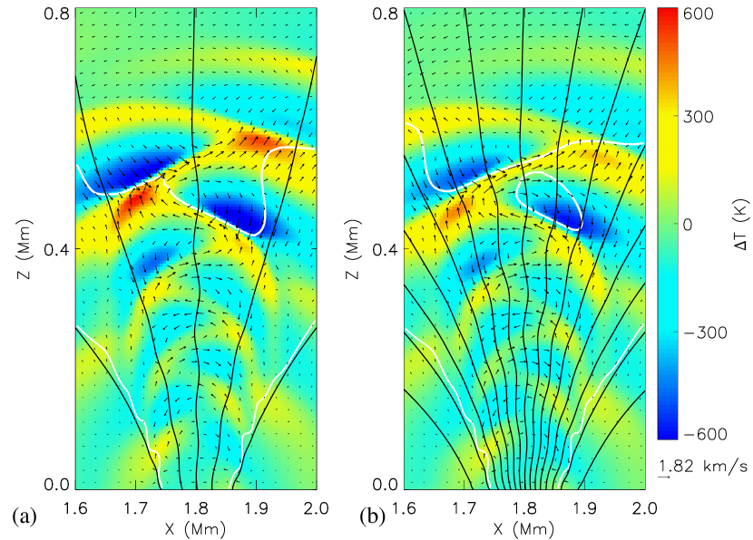
Figure 6: Close-up of the temperature perturbation $\Delta T$ and velocity field at time $t=101$ s for (a) the central flux tube shown in Fig. 4, and (b) the single flux tube shown in Fig. 3. The black curves are field lines, and the white curves are contours of plasma $\beta$ (thick: $\beta=1$; thin: $\beta=10$).

Figures 5c and 5d show similar diagrams for the model with multiple tubes. In Figs. 5a and 5c we see an antisymmetric (about the axis) velocity pattern in the strong field region ($\beta\ll 1$); this pattern can be identified with the longitudinal acoustic mode. On the other hand, in Figs. 5b and 5d we see a symmetric pattern as a uniform halo, corresponding to the transverse MHD mode. There is a clear separation of the modes above the $\beta=1$ level, where the fast mode speed increases rapidly with height. The associated increase in wavelength manifests itself as an increase in the spacing of the color contours. The shape of the contours is a consequence of the Alfvén speed being maximum on the axis (at a given height). Figures 6a and 6b give a close up of the temperature perturbation $\Delta T$ and velocity pattern near the central region of the tube, corresponding to the multiple and single tube configurations, respectively. Both cases clearly show the change in the flow pattern close to the $\beta=1$ level and the anti-symmetric structure of the acoustic waves away from the tube axis.

We find that the wave patterns in the single and multiple tube cases are qualitatively similar. In both cases the acoustic and magnetic type of modes are present. Even though the initial perturbation at the base ($z=0$) is transverse, strong field aligned motions develop particularly close to the central region of the tube, similar to the finding in Paper I for a single tube, which suggests that this is a general feature of the network.

5 Results for Wave Generation in the External Medium

So far we have examined the excitation of waves in flux tubes due to transverse motions of their footpoints. We now investigate the situation when the source of waves is in the field free medium, and we consider how the waves interact with the flux tube in order to assess how effectively they penetrate into flux tubes and heat the network. Let us consider a localised source that generates acoustic waves due to vertical periodic motions. The acoustic source is located at the lower boundary of the model ($z=0$) and has a Gaussian profile in $x$ with a $1/e$-width of 50 km. As before, we take the amplitude of the motions as 750 m s^-1 and period as 24 s. As we shall see the nature of wave excitation in the tube depends on the “angle of attack” or the angle between the direction of the wave front and a field line. We treat two cases corresponding to distant and near acoustic sources on the lower boundary.

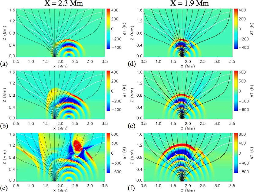
Figure 7: Temperature perturbation, $\Delta T$, (about the initial state) at (a) 76 s, (b) 101 s and (d) 140 s in a single tube due to a localised vertical periodic motion at $z=0$, $x=2300$ km (panels a- c) and $x=1900$ km (panels d- f) with an amplitude of 750 m s^-1, and a period of 24 s. The black curves denote the magnetic field lines, and the white curves are contours of constant $\beta$, corresponding to $\beta=0.1$, 0.3 and 1.0.

First consider an acoustic source at $x=2.3$ Mm, which is 500 km away from the axis of the flux rope. Figures 7(a)-(c) show the temperature perturbations at different epochs, corresponding to $t=76$ s, 101 s and 140 s respectively. It is seen that the acoustic wave strikes the tube ($\beta\approx 1$ surface) almost normal to the field and generates a fast MHD wave in the tube; for a more thorough description of what happens at this interface, see the lower panel in Fig. 3 of Cally (2007). There is also slow magnetoacoustic wave generated that essentially travels along the field lines. Figures 7(b)-(c) shows the distortion of the wave front as the wave propagates into the low $\beta$ region and where it is refracted upwards (away from the tube axis). A more informative way to examine the nature of the waves is to plot the longitudinal and transverse velocity components, which is shown for the present case in Figures 8(a)-(b) at time $t=140$ s (for $B>20$ G). The field aligned component $V_{s}$, that essentially depicts the acoustic wave, does not penetrate significantly into the central regions of the tube as we see from Figure 8(a). On the other hand, the normal component $V_{n}$, associated with the fast MHD mode (where the $\beta<1$) dominates in the central regions of the tube. This wave is generated due to mode conversion when the acoustic wave strikes the $\beta=1$ surface.

Now consider an acoustic source at $x=1.9$ Mm, only 100 km from the flux tube axis. The vertical field $B_{z}(x,0)$ at the base has a nearly Gaussian profile with $1/e$-width of 65 km, and the acoustic source has $1/e$-width of 50 km, so there is significant overlap between the two profiles. Figures 7(d)-(f) show the temperature perturbation for $t=76$ s, 101 s and 140 s, respectively. In contrast to the previous case, such a source excites waves that travel with almost no distortion by the flux tube, as can be seen by the fact that the wave front remains close to circular. From Figures 7(e) we find that the angle between the wave vector and the field lines is very small at the $\beta=1$ level. In this case, there is only a small amount of mode conversion into a transverse magnetic mode. In the magnetized region ($B>20$ G), the waves are dominantly field-aligned, as can be seen in Figures 8(c)-(d) at time $t=140$ s, which show the field-aligned and normal components of the velocity. In the region with $\beta<1$ these waves are slow magnetoacoustic modes, and the fast mode has much less power.

6 Summary and Discussion

Recent observations of the chromospheric network were discussed. We argued that Ca II network grains represent plasma located at heights between about 0.5 Mm and 1.5 Mm, and are distinct from the spicule-like features observed at larger heights (see Fig. 2). The heating in network grains must occur in a sustained (as opposed to intermittent) manner. The physical processes involved in this heating are not well understood. Long-period waves are thought to be involved in driving spicules (e.g., De Pontieu et al., 2004), but we argued against long-period waves as the cause of the heating in Ca II network grains. Instead, our hypothesis in this paper is that the heating in network grains is caused by weaker shocks that occur repetitively at short time intervals ($P<100$ s) to maintain the enhanced temperature of the network grains. The weakness of the shocks is needed to explain the observed symmetrical shapes of the Ca II H & K line profiles from network grains. The symmetry of the line profiles and relative constancy of the Ca II emission may be explained if the shocks have small horizontal scales (a few hundred km) and multiple shocks are superposed along the line of sight. At present there is no observational evidence for such short-period waves in network elements.

We studied the propagation of short-period magnetoacoustic waves in magnetic elements, using the 2-D MHD model presented in Paper I. The waves are launched as transverse kink waves at the base of the photospheric flux tubes. The present work complements Paper I in two important respects: (a) we consider an equilibrium model with lower magnetic field strength, so that the $\beta=1$ surface is located in the upper photosphere; (b) we examine the interactions of waves from neighboring tubes. We have identified an efficient mechanism for the generation of longitudinal motions in the chromosphere from purely transverse motions at the base of tubes. These longitudinal motions are associated with slow magnetoacoustic waves that can contribute to a localized heating of the chromosphere.

The qualitative features of the results for a single flux tube are similar to those found in Paper I. Irrespective of whether the field at the base of the flux tube is strong or weak, the transverse waves at the base are converted at chromospheric heights into two sets of slow-mode shocks that are 180^∘ out of phase with each other and propagate upward along the magnetic field lines on opposite sides of the flux tube axis. We propose that network grains are heated by dissipation of such shocks. This heating occurs mainly in the central part of the flux tube. We also considered an equilibrium configuration with multiple tubes, and found that through the interference of waves emanating from neighboring tubes, there is some heating at the tube interfaces. However, the dominant heating occurs near the tube axes.

For the case of a single flux tube we found that the width of the shocked region at time $t=153$ s is about 1200 km (see Fig. 3c), a significant fraction of the assumed width the flux tube at large height. For the case with multiple flux tubes, the width of the shocked region is about 900 km, or 3/4 of the width of one flux tube (see Fig. 4c). Therefore, the spatial extent of the shocked region in our models is larger than the subarcsecond size of the Ca II H network grains observed by DOT (see Fig. 1c). Part of the difference may be explained by the fact that the Ca II H images contain a significant photospheric contribution (Rutten, 2006, 2007), which originates at lower heights where the flux tubes are thinner. Another possible explanation lies in the details of spectral line formation: as the shocks propagate to larger height, the density behind the shocks decreases and the Ca II H line source function drops below the Planck function, producing the “absoption” feature at line center. Therefore, the chromospheric contribution to the observed emission comes from a limited range of heights, and may reflect only the lower part of the shocked region shown in Figures 3c and 4c. To determine whether the proposed models can explain the observed widths of network grains, more detailed modeling of the formation of the Ca II H line is needed.

We also investigated the interaction of a flux tube with acoustic waves from the external medium. A careful investigation shows that their penetration into the tube depends on the angle between the wave front and field lines, or “angle of attack” (Carlsson & Bogdan, 2006; Cally, 2007, and references therein). Schunker & Cally (2006) and Cally (2007) examined the interaction between an acoustic wave and a magnetic field, and found that at the level where the sound and Alfvén speeds are equal there is both mode transmission and mode conversion. The former refers only to a nomenclature change as a fast wave in the ambient medium is transmitted as a slow wave in the flux tube. However, the transmitted wave continues to be acoustic in character. On the other hand, in the latter case, the wave entering the magnetic medium remains fast throughout and changes character from acoustic in the ambient medium to magnetic in the flux tube, which corresponds to a mode conversion. We examined this phenomenon by considering two limiting cases of distant and near acoustic sources. Our calculations clearly show that acoustic waves, generated in the ambient medium, do not significantly penetrate inside the flux tube unless the acoustic source is located in its immediate vicinity (i.e., within about one flux tube radius). Consequently, short-period waves from the external medium do not offer a promising mechanism for heating the magnetic network at heights below 1500 km.

Future observations with Hinode/SOT should be able to establish whether short-period magnetoacoustic waves exist in flux elements at the heights where the Ca II ${\rm H}_{2V}$ and ${\rm H}_{2R}$ emission features are formed, and if so, whether they play a significant role in chromospheric heating. If such waves are not found, Alfvén waves may provide an alternative, but such waves may be difficult to detect in solar disk observations. Future modeling should consider the interactions of waves with magnetic flux tubes in three dimensions in order to allow for the coupling between all three MHD wave modes. The models should include a more realistic energy equation than the one considered here. Both p-mode waves and waves generated locally at the base of the flux tubes should be considered. Based on such models, Ca II H and K profiles should be simulated to determine whether the models can reproduce the observed symmetrical profiles from network grains.

Table 1: Parameters on the Tube Axis & Ambient Medium

	Tube Axis			Ambient Medium
Variable	$z=0$	$z=1500$ km		$z=0$	$z=1500$ km
Temperature	4700 K	8700 K		4700 K	8700 K
Density	2.6 10-7 g cm-3	2.1 10-12 g cm-3		3.9 10-7 g cm-3	3.2 10-12 g cm-3
Pressure	8.0 104 dyn cm-2	2.2 dyn cm-2		1.2 105 dyn cm-2	3.3 dyn cm-2
Sound speed	7.1 km s-1	13 km s-1		7.1 km s-1	13 km s-1
Alfvén speed	5.6 km s-1	85 km s-1		$\cdots$	$\cdots$
Magnetic field	1000 G	44 G		$\cdots$	$\cdots$
$\beta$	2.0	2.8 10-2		$\cdots$	$\cdots$

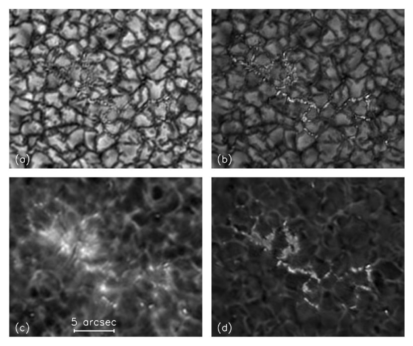
Figure 1: Dutch Open Telescope (DOT) observations of a magnetic network patch in the solar photosphere and chromosphere. The images were taken at solar disk center on 2007 April 12 at 9:35 UT. (a) blue continuum; (b) G band at 4305 Å; (c) Ca II H line center; (d) Ca II H offband (-2.35 Å). The network patch consists of many small flux elements of sub-arcsecond size. The bright network grains seen in the Ca II H line center image coincide with G-band bright points, indicating that the chromospheric heating is localized directly above the photospheric flux elements. The Ca II network grains are more diffuse than the G-band bright points, which may be due to the spreading of flux tubes with height.

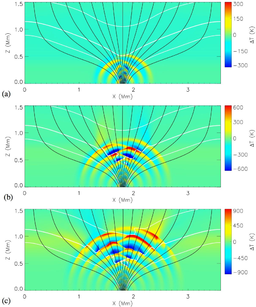
Figure 3: The temperature perturbation, $\Delta T$, (about the initial state) at (a) 75 s, (b) 122 s, and (c) 153 s in a network element due to periodic horizontal motion at the lower boundary, with an amplitude of 750 m s^-1, and a period of 24 s. The black curves denote the magnetic field lines, and the color scale shows the temperature perturbation. The white curves denote contours of constant $\beta$ corresponding to $\beta=0.1$ (upper curve), 1.0 (thick curve) and 10 (lower curve).

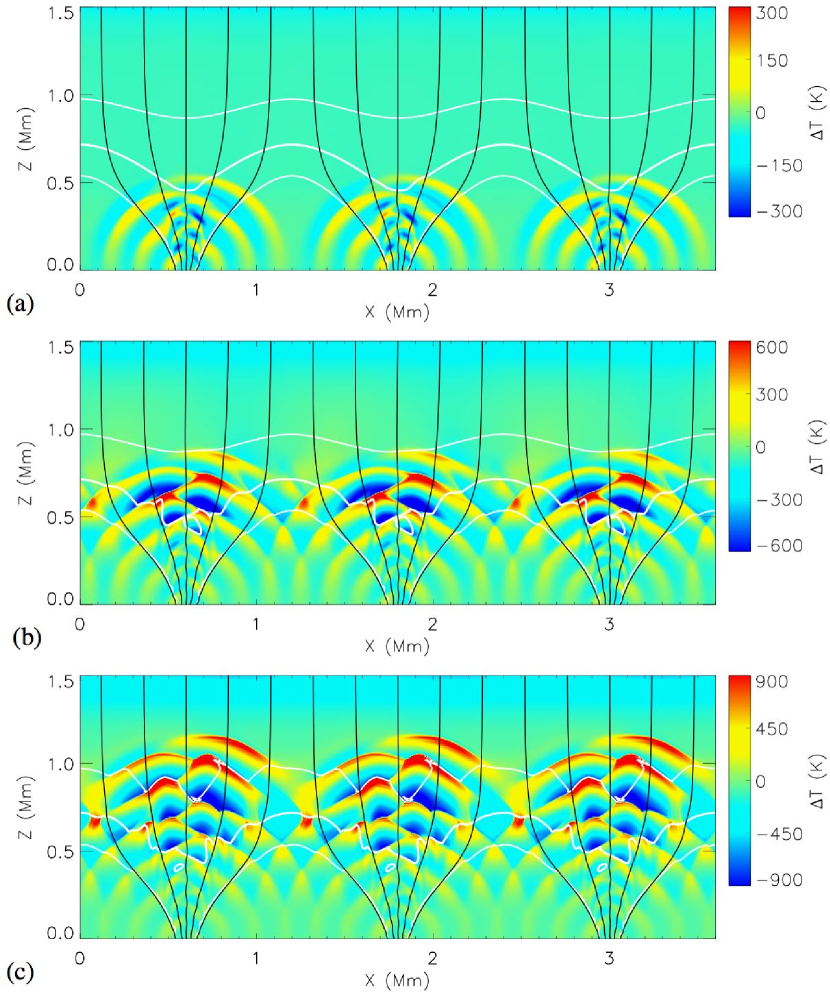
Figure 4: The temperature perturbation, $\Delta T$, (about the initial state) at (a) 75 s, (b) 122 s, and (c) 153 s in a network region consisting of 3 flux tubes. Wave excitation is due to periodic horizontal motion at the lower boundary, with an amplitude of 750 m s^-1, and a period of 24 s. The black curves denote the magnetic field lines, and the color scale shows the temperature perturbation. The white curves denote contours of constant $\beta$ corresponding to $\beta=0.1$ (upper curve), 1.0 (thick curve) and 10 (lower curve). This figure is also available as an mpeg animation in the online version of the journal.

Figure 5: Field aligned ($V_{s}$) and transverse ($V_{n}$) components of the velocity in a single tube, (panels a - b) and multiple tubes (panels c - d) at $t=120$ s due to periodic horizontal motion at the lower boundary, with an amplitude of 750 m s^-1, and a period of 24 s. The black curves are magnetic field lines, and the white curves are contours of constant $\beta$, corresponding to $\beta=0.1$, 1.0 and 10. In the weak-field region ($B<20$ G) the decomposition of velocity into field-aligned and transverse components is ambiguous, and is not shown.

References

- Berger et al. (1995) Berger, T. E., Schrijver, C. J., Shine, R. A., et al., 1995, ApJ, 454, 531
- Berger et al. (1998) Berger, T. E., Löfdahl, M. G., Shine, R. S., et al., 1998, ApJ, 495, 973
- Berger et al. (2004) Berger, T. E., Rouppe van der Voort, L. H. M., Löfdahl, M. G., Carlsson, M., Fossum, A., Hansteen, V., Marthinussen, E., Title, A., & Scharmer, G. 2004, A&A, 428, 613
- Berger & Title (1996) Berger, T. E., & Title, A. M. 1996, ApJ, 463, 365
- Bogdan et al. (2003) Bogdan, T. J., Carlsson, M., Hansteen, V., McMurry, A., Rosenthal, C. S., Johnson, M., Petty-Powell, S., Zita, E. J., Stein, R. F., McIntosh, S. W., & Nordlund, Å. 2003, ApJ, 599, 626
- Bloomfield et al. (2006) Bloomfield, D. S., McAteer, R. T., Mathioudakis, M., & Keenan, F. P. 2006, ApJ, 652, 812
- Cally (2007) Cally, P. S. 2007, Astron. Nach., 328, 286
- Carlsson & Bogdan (2006) Carlsson, M., & Bogdan, T. J., 2006, Roy. Soc. Phil. Trans., Series A, Vol. 364, p. 395
- Carlsson & Stein (1997) Carlsson, M., & Stein, R. F. 1997, ApJ, 481, 500
- Cauzzi et al. (2007) Cauzzi, G., Reardon, K. P., Uitenbroek, H., Cavallini, F., Falchi, A., Falciani, R., Janssen, K., Timmele, T., Vecchio, A., & Wöger, F. 2007, eprint arXiv:0709.2417
- Choudhuri et al. (1993) Choudhuri, A. R., Auffret, H., & Priest, E. R. 1993, Sol. Phys., 143, 49
- Cram & Damé (1983) Cram, L. E., & Damé, L. 1983, ApJ, 272, 355
- Cranmer & van Ballegooijen (2005) Cranmer, S. R., & van Ballegooijen, A. A. 2005, ApJS, 156, 265
- Cranmer et al. (2007) Cranmer, S. R., van Ballegooijen, A. A., & Edgar, R. J. 2007, ApJS, 171, 520
- De Pontieu et al. (2004) De Pontieu, B., Erdélyi, R., & James, S. P. 2004, Nature, 430, 536
- De Pontieu et al. (2005) De Pontieu, B., Erdélyi, R., & De Moortel, I. 2005, ApJ, 624, L61
- De Pontieu et al. (2007a) De Pontieu, B., Hansteen, V. H., Rouppe van der Voort, L., van Noort, M., & Carlsson, M. 2007a, ApJ, 655, 624
- De Pontieu et al. (2007b) De Pontieu, B., McIntosh, S., Hansteen, V. H., Carlsson, M., Schrijver, C. J., Tarbell, T. D., Title, A. M., Shine, R. A., Suematsu, Y., Tsuneta, S., Katsukawa, Y., Ichimoto, K., Shimizu, T., & Nagata, S. 2007b, PASJ, ??? [A tale of of two spicules]
- De Pontieu et al. (2007c) De Pontieu, B., McIntosh, S., Carlsson, M., Hansteen, V. H., Tarbell, T. D., Schrijver, C. J., Title, A. M., Shine, R. A., Tsuneta, S., Katsukawa, Y., Ichimoto, K., Suematsu, Y., Shimizu, T., & Nagata, S. 2007c, Science, 318, 1574
- Fawzy et al. (2002) Fawzy D., Rammacher, W., Ulmschneider, P., Musielak, Z.E., Stepien, K. 2002, A&A, 386, 971
- Gaizauskas (1985) Gaizauskas, V. 1985, in Chromospheric Diagnostics and Modeling, ed. B. W. Lites (National Solar Observatory: Sunspot, NM), 25
- Heggland, De Pontieu & Hansteen (2007) Heggland, L., De Pontieu, B., & Hansteen, V. H. 2007, ApJ, 666, 1277
- Hansteen et al. (2006) Hansteen, V. H., De Pontieu, B., Rouppe van der Voort, L., van Noort, M., & Carlsson, M. 2006, ApJ, 647, L73
- Hasan & Kalkofen (1999) Hasan, S. S., & Kalkofen, W. 1999, ApJ, 519, 899
- Hasan et al. (2000) Hasan, S. S., Kalkofen, W., & van Ballegooijen, A. A. 2000, ApJ, 535, L67
- Hasan et al. (2003) Hasan, S. S., Kalkofen, W., van Ballegooijen, A. A., & Ulmschneider, P. 2003, ApJ, 585, 1138
- Hasan et al. (2005) Hasan, S. S., van Ballegooijen, A. A., Kalkofen, W., & Steiner, O. 2005, ApJ, 631, 1270 (Paper I)
- Hasan et al. (2006) Hasan, S. S., Vigeesh, G., & van Ballegooijen, A. A. 2006, in Solar Activity and its Magnetic Origin, Proc. 233rd IAU Symp., eds. V. Bothmer, A. A. Hady (Cambridge: Cambridge University Press), 116
- Jefferies et al. (2006) Jefferies, S. M., McIntosh, S. W., Armstrong, J. D.. Bogdan, T. J., Cacciani, A., Fleck, B. 2006, ApJ, 648, L151
- Judge et al. (2001) Judge, P. G., Tarbell, T. D., & Wilhelm, K. 2001, ApJ, 554, 424
- Kontogiannis et al. (2006) Kontogiannis, G., Bloomfield, D. S., McAteer, R. T. J., Mathioudakis, M., Antonopoulou, E. 2006, in CP848, Recent Advances in Astronomy and Astrophysics, 7th Intl. Conf. of the Hellenic Astron. Soc., ed. N. H. Solomos (Amer. Inst. of Phys.), p. 229
- Kosugi et al. (2007) Kosugi, T., Matsuzaki, K., Sakao, T., Shimizu, T., Sone, Y., Tachikawa, S., Hashimoto, T., Minesugi, K., Ohnishi, A., Yamada, T., Tsuneta, S., Hara, H., Ichimoto, K., Suematsu, Y., Shimojo, M., Watanabe, T., Davis, J.M., Hill, L.D., Owens, J.K., Title, A.M., Culhane, J.L., Harra, L., Doschek, G.A., and Golub, L. 2007, Sol. Phys., 243, 3
- Krijger et al. (2001) Krijger, J. M., Rutten, R. J., Lites, B. W., et al. 2001, A&A, 379, 1052
- Langangen et al. (2007) Langangen, Ø., Carlsson, M., & Rouppe van der Voort, L. 2007, ApJ, 655, 615
- Lites et al. (1993) Lites, B. W., Rutten, R. J., & Kalkofen, W. 1993, ApJ, 414, 345
- Lites et al. (2007) Lites, B., Socas-Navarro, H., Kubo, M., Berger, T. E., Frank, Z., Shine, R. A., Tarbell, T. D., Title, A. M., Ichimoto, K., Katsukawa, Y., Tsuneta, S., Suematsu, Y., Shimizu, T., & Nagata, S. 2007, PASJ, 59, S571
- Lites et al. (2008) Lites, B., Kubo, M., Socas-Navarro, H., Berger, T. E., Frank, Z., Shine, R. A., Tarbell, T. D., Title, A. M., Ichimoto, K., Katsukawa, Y., Tsuneta, S., Suematsu, Y., Shimizu, T., & Nagata, S. 2008, ApJ, 672, 1237
- McIntosh & Judge (2001) McIntosh, S. W., & Judge, P. G. 2001, ApJ, 561, 420
- McIntosh & Jefferies (2006) McIntosh, S. W., & Jefferies, S. M. 2006, ApJ, 647, L77
- Muller & Roudier (1992) Muller, R., & Roudier, Th. 1992, Sol. Phys., 141, 27
- Muller et al. (1994) Muller, R., Roudier, Th., Vigneau, J., & Auffret, H. 1994, A&A, 283, 232
- Nisenson et al. (2003) Nisenson, P., van Ballegooijen, A. A., de Wijn, A. G., & Sütterlin, P. 2003, ApJ, 587, 458
- Oran & Boris (1987) Oran, E. S., & Boris, J. P. 1987, Numerical Simulations of Reactive Flow (New York: Elsevier)
- Rezaei et al. (2007) Rezaei, R., Steiner, O., Wedemeyer-Böhm, S., Schlichenmaier, R., Schmidt, W., & Lites, B. W. 2007, A&A, 476, L33
- Roberts & Webb (1978) Roberts, B. & Webb, A. R. 1978, Sol. Phys., 56, 5
- Rosenthal et al. (2002) Rosenthal, C. S., Bogdan, T. J., Carlsson, M., Dorch, S. B. F., Hansteen, V., McIntosh, S. W., McMurry, A., Nordlund, Å., & Stein, R. F. 2002, ApJ, 564, 508
- Rouppe van der Voort et al. (2005) Rouppe van der Voort, L. H. M., Hansteen, V.H., Carlsson, M., et al., 2005, A&A, 435, 327
- Rouppe van der Voort et al. (2007) Rouppe van der Voort, L. H. M., De Pontieu, B., Hansteen, V.H., Carlsson, M., & van Noort, M. 2007, ApJ, 660, L169
- Rutten & Uitenbroek (1991) Rutten, R. J., & Uitenbroek, H. 1991, Sol. Phys., 134, 15
- Rutten (2006) Rutten, R. J. 2006, in Solar MHD: Theory and Observations, Proc. NSO Workshop 23, eds. J. Leibacher, H. Uitenbroek, & R. J. Stein, ASP Conf. Ser. 354 (San Francisco: ASP), p. 276
- Rutten (2007) Rutten, R. J. 2007, in The Physics of Chromospheric Plasmas, eds. P. Heinzel, I. Dorotovic, & R. J. Rutten, ASP Conf. Ser. 368 (San Francisco: ASP), p. 27
- Rutten et al. (2005) Rutten, R., Bettonvil, J. F. C. M., Hammerschlag R.H. et al. 2005, in Multi-Wavelength Investigations of Solar Activity, eds. A.V. Stepanov, E.E. Benevolenskaya, A.G. Kosovichev, IAU Symposium (Cambridge), 223, 597
- Schaffenberger et al. (2006) Schaffenberger, W., Wedemeyer-Böhm, S., Steiner, O., & Freytag, B. 2006, in Solar MHD: Theory and Observations: A High Spatial Resolution Perspective, ASP Conf. Ser. Vol. 354, eds. J. Leibacher, R. F. Stein, and H. Uitenbroek (San Francisco: ASP), 345
- Schunker & Cally (2006) Schunker, H., & Cally, P. S. 2006, MNRAS, 372, 551
- Sheminova et al. (2005) Sheminova, V. A., Rutten, R. J., & Rouppe van der Voort, L. H. M. 2005, A&A, 437, 1069
- Simon & Leighton (1964) Simon, G. W., & Leighton, R. B. 1964, ApJ, 140, 1120
- Spruit (1981) Spruit, H. C. 1981, A&A, 102, 129
- Steiner et al. (1994) Steiner, O., Knölker, M. & Schüssler, M. 1994, in Solar Surface Magnetism, eds. R. J. Rutten & C. J. Schrijver, NATO ASI Ser. C-433 (Dordrecht: Kluwer), p. 441
- Tritschler et al. (2007) Tritschler, A., Schmidt, W., Uitenbroek, H., & Wedemeyer-Böhm, S. 2007, A&A, 462, 303
- Tsuneta et al. (2007) Tsuneta, S., Suematsu, Y., Ichimoto, K., Shimizu, T., Otsubo, M., Nagata, S., Katsukawa, Y., Title, A., Tarbell, T., Shine, R., Rosenberg, B., Hoffmann, C., Jurcevich, B., Levay, M., Lites, B., Elmore, D., Matsushita, T., Kawaguchi, N., Mikami, I., Shimada, S., Hill, L., and Owens, J. 2007, Sol. Phys., in press
- Ulmschneider (2003) Ulmschneider, P. 2003, in Lectures on Solar Physics, eds. Antia H. M., Bhatnagar A., & Ulmschneider P., Lecture Notes in Physics 619, Springer Verlag, Heidelberg, Berlin, p. 232
- van Ballegooijen & Nisenson (1998) van Ballegooijen, A. A., & Nisenson, P. 1998, in High Resolution Solar Physics: Theory, Observations, and Techniques, eds. T. R. Rimmele, K. S. Balasubramaniam, & R. R. Radick, ASP Conf. Ser. 183 (San Francisco: ASP), 30
- Vecchio et al. (2007) Vecchio, A., Cauzzi, G., Reardon, K. P., Janssen, K., & Rimmele, T. 2007, A&A, ???
- Vögler et al. (2005) Vögler, A., Shelyag, S., Schüssler, M., Cattaneo, F., Emonet, T. 2005, A&A, 429, 335
- Zhugzhda et al. (1995) Zhugzhda, Y. D., Bromm, V., & Ulmschneider, P. 1995, A&A, 300, 302
- Zwaan (1987) Zwaan, C. 1987, ARA&A, 25, 83