Sensitivity analysis of the solar rotation to helioseismic data from GONG, GOLF and MDI observations.

Abstract

Accurate determination of the rotation rate in the radiative zone of the sun from helioseismic observations requires rotational frequency splittings of exceptional quality as well as reliable inversion techniques. We present here inferences based on mode parameters calculated from 2088-days long MDI, GONG and GOLF time series that were fitted to estimate very low frequency rotational splittings ($\nu<1.7$ mHz). These low frequency modes provide data of exceptional quality, since the width of the mode peaks is much smaller than the rotational splitting and hence it is much easier to separate the rotational splittings from the effects caused by the finite lifetime and the stochastic excitation of the modes.

We also have implemented a new inversion methodology that allows us to infer the rotation rate of the radiative interior from mode sets that span $\ell=1$ to 25. Our results are compatible with the sun rotating like a rigid solid in most of the radiative zone and slowing down in the core ($r/R_{\odot}<0.2$). A resolution analysis of the inversion was carried out for the solar rotation inverse problem. This analysis effectively establishes a direct relationship between the mode set included in the inversion and the sensitivity and information content of the resulting inferences. We show that such an approach allows us to determine the effect of adding low frequency and low degree $p$-modes, high frequency and low degree $p$-modes, as well as some $g$-modes on the derived rotation rate in the solar radiative zone, and in particular the solar core. We conclude that the level of uncertainties that is needed to infer the dynamical conditions in the core when only $p$-modes are included is unlikely to be reached in the near future, and hence sustained efforts are needed towards the detection and characterization of $g$-modes.

1 Introduction

Over the past decade, increasingly accurate helioseismic observations from ground-based and space-based instruments have given us a reasonably good description of the dynamics of the solar interior (e.g. Schou et al., 1998; Thompson, Christensen-Dalsgaard, Miesch, & Toomre, 2003). Helioseismic inferences have confirmed that the differential rotation observed at the surface persists throughout the convection zone. There appears to be very little, if any, variation of the rotation rate with latitude in the outer radiative zone ($0.4>r/R_{\odot}>0.7$). In that region the rotation rate is almost constant ($\approx 430$ nHz), while at the base of the convection zone, a shear layer —known as the tachocline— separates the region of differential rotation throughout the convection zone from the one with rigid rotation in the radiative zone.

Despite the large scatter amongst the rotational splittings that are sensitive to the solar core (see discussion in Eff-Darwich, Korzennik, & Jiménez-Reyes, 2002), we can rule out an inward increase or decrease of the solar internal rotation rate down to $r/R_{\odot}\approx 0.25$, by more than $20\%$ of the surface rate at mid-latitude (Chaplin et al., 1999; Eff-Darwich, Korzennik, & Jiménez-Reyes, 2002; Couvidat et al., 2003). This is in clear disagreement with the theoretical hydrodynamical models that predict a much faster rotation in the solar core, namely 10 to 50 times faster than the surface rate (e.g. Thompson, Christensen-Dalsgaard, Miesch, & Toomre, 2003).

More recently, Garcia et al. (2004) and Korzennik (2005) have independently developed new mode fitting procedures to improve the quality and precision of the characterization of the modes that are sensitive to the rotation in the solar core. By using very long time series —spanning nearly six years of observations— collected with the MDI (Scherrer et al., 1995), GONG (Harvey et al., 1996) and GOLF (Gabriel et al., 1995) instruments they have measured rotational splittings for modes with frequencies as low as $1.1$ mHz.

We present here an attempt to constraint the radial and latitudinal distribution of the rotation rate in the radiative interior through the inversion of a combined MDI, GONG & GOLF data set. We also attempt to establish the sensitivity of helioseismic data sets to the dynamics of the inner solar radiative interior, as well as the level of accuracy that helioseismic data should have to resolve the solar core.

2 Theoretical background

The starting point of all linear rotational helioseismic inversion methodologies is the functional form of the perturbation in frequency, $\Delta\nu_{n\ell m}$, induced by the rotation of the sun, $\Omega(r,\theta)$, and given by (see derivation in Hansen et al., 1977):

$$\Delta\nu_{n\ell m}=\frac{1}{2\pi}\int_{0}^{R}\int_{0}^{\pi}K_{n\ell m}(r,\theta)\Omega(r,\theta)drd\theta\pm\epsilon_{n\ell m}$$ (1)

The perturbation in frequency, $\Delta\nu_{n\ell m}$, with the observational error, $\epsilon_{n\ell m}$, that corresponds to the rotational component of the frequency splittings, is given by the integral of the product of a sensitivity function, or kernel, $K_{n\ell m}(r,\theta)$, with the rotation rate, $\Omega(r,\theta)$, over the radius, $r$, and the co-latitude, $\theta$. The kernels, $K_{n\ell m}(r,\theta)$, are known functions of the solar model.

Equation 1 defines a classical inverse problem for the sun’s rotation. The inversion of this set of $M$ integral equations – one for each measured $\Delta\nu_{n\ell m}$ – allows us to infer the rotation rate profile as a function of radius and latitude from a set of observed rotational frequency splittings (hereafter referred as splittings).

The inversion method we use is based on the Regularized Least-Squares methodology (RLS). The RLS method requires the discretization of the integral relation to be inverted. In our case, Eq. 1 is transformed into a matrix relation

$$D=Ax+\epsilon$$ (2)

where $D$ is the data vector, with elements $\Delta\nu_{n\ell m}$ and dimension $M$, $x$ is the solution vector to be determined at $N$ model grid points, $A$ is the matrix with the kernels, of dimension $M\times N$ and $\epsilon$ is the vector containing the corresponding observational uncertainties.

The RLS solution is the one that minimizes the quadratic difference $\chi^{2}=|Ax-D|^{2}$, with a constraint given by a smoothing matrix, $H=G^{T}G$, introduced in order to lift the singular nature of the problem (see, for additional details, Eff-Darwich & Pérez-Hernández, 1997). The matrix $G$ represents the first-order discrete differential operator, although it will be shown below that the inversion technique we have developed is to a first order approximation independent of the choice of $G$. The general relation to be minimized is

$$S(x)=(Ax-D)^{T}(Ax-D)+\gamma xHx$$ (3)

where $\gamma$ is a scalar introduced to give a suitable weight to the constraint matrix $H$ on the solution. Hence, the function $x$ is approximated by

$$x_{\rm est}=(A^{T}A+\gamma H)^{-1}A^{T}D$$ (4)

Replacing $D$ from Eq. 2 we obtain

$$x_{\rm est}=(A^{T}A+\gamma H)^{-1}A^{T}Ax\stackrel{{\scriptstyle\mathrm{def}}}{{=}}Rx$$ (5)

hence

$$R=(A^{T}A+\gamma H)^{-1}A^{T}A$$ (6)

The matrix $R$, that combines forward and inverse mapping, is referred to as the resolution or sensitivity matrix (Friedel, 2003). Ideally, $R$ would be the identity matrix, which corresponds to perfect resolution. However, if we try to find an inverse with a resolution matrix $R$ close to the identity, the solution is generally dominated by the noise magnification. The individual columns of $R$ display how anomalies in the corresponding model are imaged by the combined effect of measurement and inversion. In this sense, each element $R_{ij}$ reveals how much of the anomaly in the $j^{th}$ inversion model grid point is transferred into the $i^{th}$ grid point. Consequently, the diagonal elements $R_{ii}$ states how much of the information is saved in the model estimate and may be interpreted as the resolvability or sensitivity of $x_{i}$. We defined the sensitivity $\lambda_{i}$ of the grid point $x_{i}$ to the inversion process as follows:

$$\lambda_{i}=\frac{R_{ii}}{\sum_{j=1}^{N}R_{ij}}$$ (7)

With this definition, a lower value of $\lambda_{i}$ means a lower sensitivity of $x_{i}$ to the inversion of the solar rotation. We define a smoothing vector $W$ with elements $w_{i}=\lambda_{i}^{-1}$ that is introduced in Eq. 4 to complement the smoothing parameter $\gamma$, namely

$$x_{\rm est}=(A^{T}A+\gamma WH)^{-1}A^{T}D$$ (8)

Such substitution allows to apply different regularizations to different model grid points $x_{i}$ whose sensitivities depend on the data set that are used in the inversions. In this sense, the inversion is a two steps process: first $R$ is obtained from Eq. 5 for a small value of the regularization parameter $\gamma$. Then, the smoothing vector $W$ is calculated through Eq. 7 and the inversion estimates are obtained through Eq. 8. A set of results can be calculated for different values of $\gamma$, the optimal solution being the one with the best trade-off between error propagation and the quadratic difference $\chi^{2}=|Ax_{\rm est}-D|^{2}$ as introduced in Eff-Darwich & Pérez-Hernández (1997).

In this paper we show how to use the matrix $R$ to study the sensitivity of helioseismic data sets to the rotation rate of the solar interior. Consequently, we present a theoretical analysis of the effect of adding low frequency and low degree $p$-modes, high frequency and low degree $p$-modes, and $g$-modes on the rotation rate of the solar core derived through numerical helioseismic inversion techniques.

3 Observational mode parameters and inversion results from 2088-days long MDI, GOLF and GONG time series

The work presented here is based on rotational frequency splittings measured from observations by the GONG ground-based network and the MDI and GOLF experiments on board the SOHO spacecraft. All rotational splittings were computed from 2088-days long time series, starting April 30th 1996 and ending January 17th 2002, as summarized in Table 1.

The three data sets KM, KG & GG (see Table 1 for explanations) contain for the first time very low frequency rotational splittings ($\nu<1.7$ mHz). These low frequency modes provide data of exceptional quality, since the width of the mode peaks is much smaller than the rotational splitting. It is therefore much easier to separate the rotational splittings from the effects caused by the finite lifetime and the stochastic excitation of the modes. The data set SM (see again Table 1) was obtained by averaging all the data sets resulting from fitting the 72-days long MDI time series (Schou et al., 1998) that overlap the April 30th 1996 to January 17th 2002 period. The averaging process reduces significantly the number of $\ell<8$ modes in that data set.

Since these data sets have been calculated from different time-series and peak-fitting techniques, one can expect some differences among the different data sets. When using different time-series, the mode parameters can be affected by the changing solar activity cycle. Moreover, fitting techniques can give different results if they are applied to either individual peaks or to ridges (Korzennik, 2005). Differences between MDI, GOLF and GONG can also arise from systematics introduced by the merging process used by GONG to obtain single time-series from multiple stations located worldwide. Differences may also come from the different spatial filters and leakage matrices that are used to isolate the signal of an individual mode (Korzennik, 2005; Chaplin et al., 2006). In any case, we combined the various data sets in a single set – following the prescription described in Table 2. Our newly developed inversion methodology was applied to the combined set to infer the rotation rate in the solar interior.

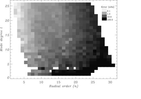
Figure 1: Observational uncertainties of the frequency splittings, shown as a function of radial order $n$ and spherical harmonic degree, $\ell$. Uncertainties obtained from 2088-days long time-series for the combined sectoral frequency splittings set are shown using a logarithmic gray scale.

Figure 1 shows the observational frequency splitting uncertainties of the combined data set as a function of radial order and degree, whereas Figs. 2 and 3 show the splittings uncertainties for sectoral modes as a function of a proxy of the inner turning point of the modes, $\ell/\nu$, and as a function of frequency, $\nu$, respectively. These plots clearly illustrate the well known and challenging fact that only a small number of modes penetrate the solar core and that the largest uncertainties are associated with these modes. Indeed, the combined data set does not include low degree high frequency modes (i.e., $\ell<4$ and $\nu>2.2$ mHz), since at higher frequencies unwanted bias appears in the estimated splittings due to the difficulty in separating the effect of rotational splitting from the limited lifetime of the modes (Appourchaux et al., 2000; Chaplin et al., 2006).

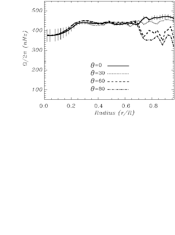
Figure 4: Inversion of the combined MDI-GOLF-GONG data set (see Table 2), plotted as a function of radius at several latitudes, $\theta$. The solid, dotted, dashed and dotted-dashed lines correspond to the rotation rate for the equator, and at latitudes of $30^{o}$, $60^{o}$ and $80^{o}$, respectively. Error bars are shown for the rotation rate at the equator, whereas the error distributions for other latitudes are shown in Fig. 12.

The inversion of the combined MDI-GOLF-GONG data (see Fig. 4) confirms that the well-known differential rotation observed at the surface persists throughout the convection zone. Although only $\ell<25$ modes were used in the inversion, it was possible to infer the rotation rate in the convection zone as the result of the exceptional quality of the low frequency splittings ($\nu<1.7$ mHz) obtained by Korzennik (2005). The differential rotation changes abruptly at approximately $0.7R_{\odot}$ to rigid rotation throughout the radiative zone. The radial distribution of the rotation is approximately flat, at a rate of $\approx 430$ nHz, decreasing below $0.2R_{\odot}$. The tendency below $0.15R_{\odot}$ is not real and results from extrapolation of the trend seen at larger radii, as explained in the following section.

4 Sensitivity analysis for the inversion of the solar radiative interior.

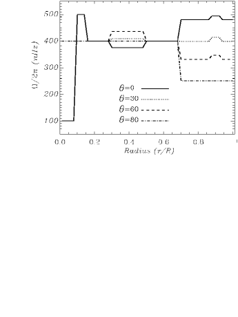
Figure 5: Artificial rotation rate for the solar interior shown as a function of radius, $r$, at different latitudes, $\theta$. This artificial profile incorporates latitudinal variations in two zones to test the inversion sensitivity to latitude. The solid, dotted, dashed and dotted-dashed correspond to the rotation rate for the equator, and at latitudes of $30^{o}$, $60^{o}$ and $80^{o}$, respectively.

A theoretical analysis was carried out in order to determine the effect of different low degree mode sets on the derivations of the solar rotation rate of the inner radiative interior. Four different artificial data sets, hereafter referred as ${\sf A}_{1}$ to ${\sf A}_{4}$ were calculated using Eq. 1 and an artificial rotation rate $\Omega_{\rm A}(r,\theta)$ that is shown in Fig. 5. The different artificial data sets correspond to different mode sets and/or uncertainties, as explained in Table 3. The observational uncertainties (standard errors) were taken from the combined mode set used in the previous section, whereas the noise added to the artificial data was calculated from normal distribution with the observed uncertainties. The ${\sf A}_{1}$ data set contains the same mode set than the combined MDI-GOLF-GONG data set. Errors for g modes were arbitrarily set to 6 nHz (the mean of the observational uncertainties for the acoustic mode splittings), since at present there are not reliable estimates for the uncertainties of g-modes frequency splittings. In any case, we are interested in the behavior of the inversion methodology when g modes are added, rather than in the results of the inversion for different values of the splittings and the observational errors.

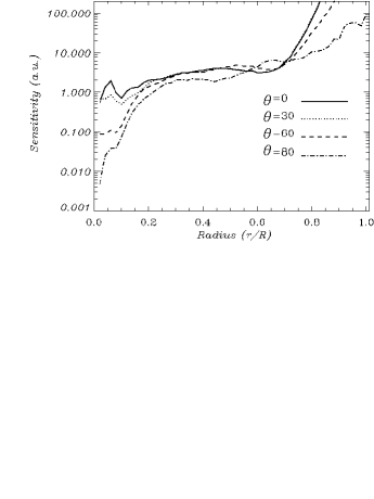
Figure 7: Sensitivities to set ${\sf A}_{4}$ of the solar rotation at different latitudes, namely the equator (solid line), $30^{o}$ (dotted lines), $60^{o}$ (dashed lines) and $80^{o}$ (dotted-dashed lines).

The sensitivity vector, $\Lambda$, was computed for the four artificial data sets, as illustrated in Figs. 6 and 7, where the sensitivities, ${\lambda_{i}}$, for the rotation rate in the solar interior are presented as a function of the radius, for each artificial data set at the equator or for several latitudes for a given set. The data sets ${\sf A}_{1}$ and ${\sf A}_{2}$ are significantly less sensitive to the rotation of the solar core than the other sets. Although the ${\sf A}_{2}$ set includes the same high frequency modes as set ${\sf A}_{3}$, the errors of the ${\sf A}_{2}$ set are significantly larger and hence the sensitivities do not differ from those obtained for the ${\sf A}_{1}$ set. The addition of two $g$-modes (in set ${\sf A}_{4}$) increases significantly the sensitivity to the solar core. However, it is important to notice that even with the addition of $g$-modes, the sensitivity at the solar core varies with the latitude, as illustrated in Fig. 7. For all sets, the sensitivities to the equatorial regions of the solar core are larger than the sensitivities at other latitudes.

The effect on the sensitivity vector of the choice of the smoothing matrix $H$ is presented in Fig. 8, where the equatorial sensitivities ${\lambda_{i}}$ for the first, second and third-order discrete differential operators $G$ are shown. The larger the order of the operator $G$ the larger the sensitivity, except near the edges, and in particular the core. The smoothing vector $W$ is obtained from the sensitivity vector $\Lambda$ and hence, the regularization constraint will not only depend on the mode set, but also on the shape of $G$.

The choice of the number and spatial distribution of the model grid points, $N$, is an important aspect of the inversion process. In non-adaptive regularization inversions, decreasing the number of grid points is in itself a form of regularization. The inversion procedure described here will also adjust to the distribution of grid points. This is illustrated in Fig. 9, where we show that the variation of the inversion sensitivities (and hence the regularization constraints) is not constant with radius and latitude when the number of grid points are changed. In this sense, the a priori choice of the distribution of model grid points will not constrain the inversion results.

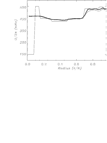
Figure 10: Inversions of set ${\sf A}_{3}$ as a function of radius at the equator. Results for the standard RLS inversion (no vector $W$) and for the newly developed inversion method are shown in dotted and solid lines, respectively. The artificial rotation rate used to calculate the input sets is shown as the thin solid line.

The inversion methodology developed for the work presented here differs from standard RLS techniques by introducing a smoothing vector $W$. The purpose of this vector is to avoid over-smoothing the inversion solution in certain regions of the solar interior and hence loose valuable information. This is illustrated in Fig. 10, where two different inversions of the same data set are presented, namely a standard RLS inversion (no vector $W$ is added) dotted line, and the newly developed RLS inversion, solid line. The standard RLS inversion tends to over-smooth and hence to assign unrealistic low errors to the estimated rotation in the convection zone to get a stable solution in the radiative regions. However when $W$ is added to the inversion procedure, the over-smoothing problem in the convection zone is mitigated, since the sensitivities ${\lambda_{i}}$ in the convection zone are larger and hence, the smoothing coefficients ${w_{i}}$ are lower. The standard RLS technique would assign the same smoothing coefficients to all model grid points in the inversion.

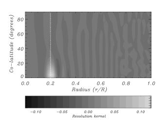
Figure 14: Plot of the resolution vector $R_{ij}$, $j=1,N$, calculated for set ${\sf A}_{3}$ corresponding to the inversion estimated at the equator but for $r_{i}=0.20R_{\odot}$ (indicated by vertical dotted lines).

The correspondence between the sensitivity analysis shown in Figs. 6 and 7 and the information contained in the resolution matrix $R$ is illustrated in Figs. 11 to 13, where we show the resolution vector corresponding to the estimate at the equator for $r_{i}=0.06R_{\odot}$. This corresponds to the averaging kernel defined by Backus & Gilbert (1970) for the Optimal Localized Averages technique. In the ideal case, the resolution should be unity at the location where the solution is estimated and zero elsewhere. Only in the inversion of the ${\sf A}_{4}$ set is the largest amplitude of the resolution vector centered at $r_{i}=0.06R_{\odot}$, and thus the result is reliable. The poor localization of the resolution at $r_{i}=0.06R_{\odot}$ for the inversions of the ${\sf A}_{1}$ to ${\sf A}_{3}$ set could not be improved by any inversion technique. However, this lack of resolution is taken into account by the sensitivity analysis, since it evaluates low sensitivities and hence assigns large regularizations to those grid points. At larger radii both the location and the amplitude of the resolution are significantly increased, as illustrated in Fig. 14, where we show the resolution corresponding to the estimate at the equator for $r_{i}=0.2R_{\odot}$ obtained with the data set ${\sf A}_{3}$.

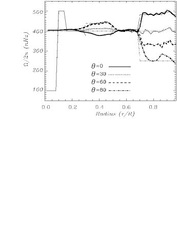
Figure 15: Inversion of set ${\sf A}_{1}$ as a function of radius at different latitudes, namely the equator (solid line), $30^{o}$ (dotted lines), $60^{o}$ (dashed lines) and $80^{o}$ (dotted-dashed lines). The artificial rotation rate used to calculate the input set is shown as thin lines.

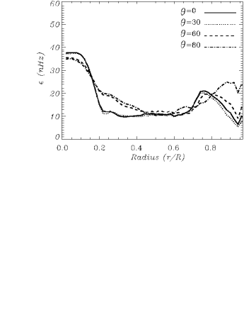
Figure 16: Error distribution for the inversion of set ${\sf A}_{1}$ as a function of radius at different latitudes, namely the equator (solid line), $30^{o}$ (dotted lines), $60^{o}$ (dashed lines) and $80^{o}$ (dotted-dashed lines).

The conclusions derived from Figs. 6 and 7 can also be drawn from the inversions of the data sets, as illustrated in Figs. 15 to 18. Figures 15 and 16 show the inverted profile and error distribution for the ${\sf A}_{1}$ set at several latitudes and demonstrates that there is good sensitivity to the latitudinal variation in the radiative rotation rate above $r\approx 0.3R_{\odot}$. Hence, the absence of differential rotation for the solar rotation rate in the radiative interior (Fig. 4) is real, not an artifact of the inversion procedure. The unrealistic flat rotation rate below $r\approx 0.15R_{\odot}$ resulting from the inversions of the ${\sf A}_{1}$ and ${\sf A}_{2}$ sets is due to the lack of sensitivity of the mode set to that region. As a result the inversion extrapolates the trend of the solution at larger radii. There are not significant differences in the inversions of sets ${\sf A}_{1}$ and ${\sf A}_{2}$, although set ${\sf A}_{2}$ includes low degree and high frequency modes. However, the new information contained in the low degree and high frequency modes of set ${\sf A}_{2}$ is lost due to they large observational uncertainties. In all four cases, larger differences between the artificial and the inverted rotation rates are seen at higher latitudes, especially in the radiative interior, as a result of the lack of sensitivity of the inversions to the polar regions.

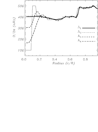
Figure 17: Inversions of set ${\sf A}_{1}$ to ${\sf A}_{4}$ plotted as a function of radius at the equator. Results for sets ${\sf A}_{1}$ to ${\sf A}_{4}$ are shown as solid, dotted, dashed and dotted-dashed lines respectively. The artificial rotation rate used to calculate the input sets is shown as a thin solid line.

Only in the cases of sets ${\sf A}_{3}$ and ${\sf A}_{4}$ (see Fig. 17), was it possible to infer the main trends of the rotation rate below $r\approx 0.15R_{\odot}$. However, it was necessary to include, either, data with unrealistic small observational errors (set ${\sf A}_{3}$), or, a couple of $g$-modes (set ${\sf A}_{4}$), modes that have yet to be unambiguously observed. The most likely way to reduce the observational uncertainties consists of increasing the length of the time series. Figure 19 compares the observational errors for the $\ell=25$ sectoral modes for five 728-days long data sets to the 2088-days long data set, all estimated by Korzennik (2005). The formal observational uncertainties are proportional to the square root of the length of the time series, hence it would be necessary to observe for decades to reduce the observational uncertainties of the very low degree modes to the current levels of the $\ell=25$ modes, all the while assuming that we can also reduce the residual bias in our current estimates of the low degree and high frequency splittings (see discussions in Appourchaux et al., 2000; Chaplin et al., 2006).

5 Conclusions

We have used for the first time a combined MDI-GOLF-GONG data set of rotational frequency splittings that covers the largest possible frequency range, spanning from 1.1 mHz to 3.9 mHz. This mode set was determined from 2088-days long time series acquired by the MDI, GOLF and GONG instruments and analyzed independently by several authors, namely Korzennik (2005), Garcia et al. (2004), Gelly et al. (2002), Schou et al. (1998) and Jiménez-Reyes (2000). Very low frequency splittings ($\nu<1.7$ mHz) were included to improve the precision and the resolution of the inversion in the solar interior.

In order to optimally invert this unique data set, we implemented a new inversion methodology that combines the regularized least-squares technique with the analysis of the sensitivity of the solution at all model grid point to the mode set being inverted. The inversion of the actual MDI-GOLF-GONG data set reveals that the sun rotates as a rigid solid in most of the radiative interior and slowing down below $0.2R_{\odot}$.

The calculation of the sensitivity vector $\Lambda$ offers a rapid and intuitive way of evaluating the sensitivity of helioseismic data to the dynamics of the solar interior, in particular in the core ($r<0.25R_{\odot}$). We conclude that with the present accuracy of the available splittings, it is not possible to derive the dynamical conditions below $r\approx 0.2R_{\odot}$. This results from the relatively large observational uncertainties of the modes sensitive to the solar core, in particular the low degree and high frequency modes. The level of uncertainties that is needed to infer the dynamical conditions in the core when only including $p$-modes is unlikely to be reached in the near future, and hence sustained efforts are needed towards the detection and characterization of $g$ modes.

6 Acknowledgments

The Solar Oscillations Investigation - Michelson Doppler Imager project on SOHO is supported by NASA grant NAS5–3077 at Stanford University. SOHO is a project of international cooperation between ESA and NASA.

The GONG project is funded by the National Science Foundation through the National Solar Observatory, a division of the National Optical Astronomy Observatories, which is operated under a cooperative agreement between the Association of Universities for Research in Astronomy and the NSF.

This work was funded by the Spanish grant AYA2004-04462. SGK was supported by NASA grants NAG5–13501 & NNG05GD58G and by NSF grant ATM–0318390.

Table 1: Description of the data sets used in this work.

Instrument	Degree	Frequency (mHz)	Reference	Referred as
MDI	$4\leq\ell\leq 25$	$1.1\leq\nu\leq 3.9$	Korzennik 2005	KM
GONG	$4\leq\ell\leq 25$	$1.1\leq\nu\leq 3.9$	Korzennik 2005	KG
MDI	$5\leq\ell\leq 25$	$1.7\leq\nu\leq 3.9$	Schou et al. 1998	SM
MDI	$1\leq\ell\leq 10$	$1.8\leq\nu\leq 3.9$	Jiménez-Reyes et al. 2000	JM
GOLF	$1\leq\ell\leq 3$	$1.1\leq\nu\leq 2.2$	García et al. 2004	GG
GOLF	$\ell=1$	$1.4\leq\nu\leq 3.9$	Gelly et al. 2002	BG

Table 2: Description of the combined data set used, and a brief description of the combination procedure.

Instrument	Degree	Frequency (mHz)	Combination Procedure
GOLF	$\ell=1$	$1.1\leq\nu\leq 2.2$	Average of GG and BG
GOLF	$\ell=2,3$	$1.1\leq\nu\leq 2.2$	Data from GG
MDI	$\ell=1,3$	$2.2<\nu\leq 3.9$	Data from JM
MDI-GONG	$4\leq\ell\leq 10$	$1.1\leq\nu\leq 1.8$	Average of KM and KG
MDI-GONG	$4\leq\ell\leq 10$	$1.8\leq\nu\leq 3.9$	Average of JM, KM, SM and KG
MDI-GONG	$11\leq\ell\leq 25$	$1.1\leq\nu\leq 1.8$	Average of KM and KG
MDI-GONG	$11\leq\ell\leq 25$	$1.8\leq\nu\leq 3.9$	Average of KM, KG and SM

The MDI-GONG-GOLF set consists of the ensemble of these values, although the MDI data for $\ell=1,3$ and $2.2<\nu\leq 3.9$ are only used to compute artificial data sets.

Table 3: Description of the artificial data sets used to study the sensitivity of helioseismic data to the dynamics of the solar core.

		Freq. range (mHz)
Data set	Note	$\ell=1$	$\ell=2,3$	$\ell>3$
Set ${\sf A}_{1}$		$1\leq\nu\leq 2.2$	$1\leq\nu\leq 2.2$	$1\leq\nu\leq 3.9$
Set ${\sf A}_{2}$		$1\leq\nu\leq 3.9$	$1\leq\nu\leq 3.9$	$1\leq\nu\leq 3.9$
Set ${\sf A}_{3}$	(1)	$1\leq\nu\leq 3.9$	$1\leq\nu\leq 3.9$	$1\leq\nu\leq 3.9$
Set ${\sf A}_{4}$	(2)	$0.1\leq\nu\leq 2.2$	$0.1\leq\nu\leq 2.2$	$1\leq\nu\leq 3.9$

⁽¹⁾ Data set ${\sf A}_{3}$ differs from data set ${\sf A}_{2}$ in its uncertainties: the uncertainties for $\ell<4$ are set to be the ones for the sectoral splittings of $\ell=25$.

⁽²⁾ One $\ell=1$ and one sectoral $\ell=2$ $g$-modes rotational splittings were added to the ${\sf A}_{1}$ data set.

Figure 2: Observational uncertainties of sectoral frequency splittings as a function of the inner turning point proxy $\ell/\nu$, for a selected set of degrees. The solid, dotted, dashed and dashed-dotted lines correspond to $\ell=25,15,5$ and $1$, respectively.

Figure 3: Observational uncertainties of sectoral frequency splittings as a function of the mode frequency, $\nu$, for a selected set of degrees. The solid, dotted, dashed and dashed-dotted lines correspond to $\ell=25,15,5$ and $1$, respectively.

Figure 6: Sensitivities of the solar rotation at the equator for sets ${\sf A}_{1}$ to ${\sf A}_{4}$, represented by solid lines, dotted lines, dashed lines, and dotted-dashed lines, respectively.

Figure 8: Sensitivities to set ${\sf A}_{1}$ of the solar rotation at the equator for three different smoothing matrices $H$, namely those corresponding to first differences (solid line), second differences (dotted lines) and third differences (dashed lines).

Figure 9: Sensitivities to set ${\sf A}_{1}$ of the solar rotation at the equator for two different distributions of model grid points, namely 50 & 16 points (solid line) and 25 & 16 points in the radial and angular directions respectively (dotted line).

Figure 11: Plot of the resolution vector $R_{ij}$, $j=1,N$, calculated for set ${\sf A}_{1}$ corresponding to the inversion estimated at the equator for $r_{i}=0.06R_{\odot}$ (indicated by vertical dotted lines). The same result was obtained for the inversion of ${\sf A}_{2}$ .

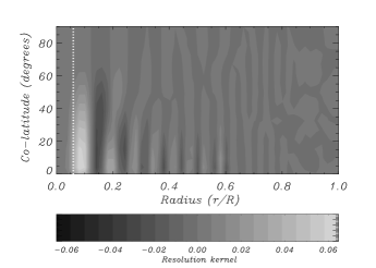
Figure 12: Plot of the resolution vector $R_{ij}$, $j=1,N$, calculated for set ${\sf A}_{3}$ corresponding to the inversion estimated, as in Fig. 11, at the equator for $r_{i}=0.06R_{\odot}$.

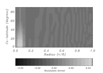
Figure 13: Plot of the resolution vector $R_{ij}$, $j=1,N$, calculated for set ${\sf A}_{4}$ corresponding to the inversion estimated , as in Figs. 11 & 12, at the equator for $r_{i}=0.06R_{\odot}$.

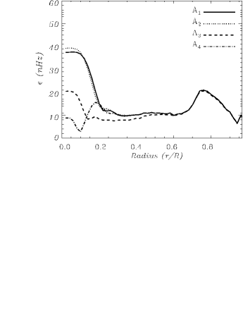
Figure 18: Error distribution for the inversions of set ${\sf A}_{1}$ to ${\sf A}_{4}$ plotted as a function of radius at the equator. Results for sets ${\sf A}_{1}$ to ${\sf A}_{4}$ are shown as solid, dotted, dashed and dotted-dashed lines respectively.

Figure 19: Observational uncertainties for $\ell=25$ sectoral frequency splittings as a function of the mode frequency, $\nu$. The solid line represents the uncertainties for the 2088-days long data set, whereas the other line styles represent the uncertainties for the five 728-days long data sets.

References

- Appourchaux et al. (2000) Appourchaux, T., Chang H. Y., Gough, D. O., Sekii, T. 2000, MNRAS, 319, 365
- Backus & Gilbert (1970) Backus G., Gilbert F. 1970, Phil. Trans. R. Soc. London 266, 123
- Chaplin et al. (1999) Chaplin, W.J., Christensen-Dalsgaard, J., Elsworth, Y., Howe, R., Isaak, G.R., Larsen, R.M., New, R., Schou, J., Thompson, M.J., & Tomczyk, S., 1999, MNRAS, 308, 405
- Chaplin et al. (2004) Chaplin, W. J., Sekii, T., Elsworth, Y., & Gough, D. O. 2004, MNRAS, 355, 535
- Chaplin et al. (2006) Chaplin, W. J., et al. 2006, MNRAS, 369, 985
- Couvidat et al. (2003) Couvidat, S., García, R. A., Turck-Chièze, S., Corbard, T., Henney, C. J., & Jiménez-Reyes, S. 2003, ApJL, 597, L77
- Eff-Darwich & Pérez-Hernández (1997) Eff-Darwich, A., Pérez-Hernández, F., 1997, A&ASS, 125, 1
- Eff-Darwich, Korzennik, & Jiménez-Reyes (2002) Eff-Darwich, A., Korzennik, S. G., & Jiménez-Reyes, S. J. 2002, ApJ, 573, 857
- Friedel (2003) Friedel, S. 2003, Geophys. J. Int., 153, 305
- Gabriel et al. (1995) Gabriel, A. H., et al. 1995, Sol. Phys., 162, 61
- Garcia et al. (2004) Garcia, R. A., et al. 2004, Sol.Phys., 220, 269
- Gelly et al. (2002) Gelly, B., Lazrek, M., Grec, G., Ayad, A., Schmider, F. X., Renaud, C., Salabert, D., & Fossat, E. 2002, A&A, 394, 285
- Hansen et al. (1977) Hansen, C.J., Cox, J.P. and van Horn, H.M., 1977, ApJ, 217, 151
- Harvey et al. (1996) Harvey, J. W., et al. 1996, Science, 272, 1284
- Jiménez-Reyes (2000) Jiménez-Reyes, S.J., 2000, Thesis Dissertation, Univ. La Laguna, Tenerife.
- Korzennik (2005) Korzennik, S.G., 2005, ApJ, 626, 585
- Scherrer et al. (1995) Scherrer, P. H., et al. 1995, Sol. Phys., 162, 129
- Schou et al. (1998) Schou, J., et al., 1998, ApJ, 505, 390
- Thompson, Christensen-Dalsgaard, Miesch, & Toomre (2003) Thompson, M. J., Christensen-Dalsgaard, J., Miesch, M. S., & Toomre, J. 2003, Ann. Rev. Astron. Astrophys., 41, 599