Molecular kinetic analysis of a finite-time Carnot cycle

Abstract

We study the efficiency at the maximal power $\eta_{\mathrm{max}}$ of a finite-time Carnot cycle of a weakly interacting gas which we can regard as a nearly ideal gas. In several systems interacting with the hot and cold reservoirs of the temperatures $T_{\mathrm{h}}$ and $T_{\mathrm{c}}$, respectively, it is known that $\eta_{\mathrm{max}}=1-\sqrt{{T_{\mathrm{c}}}/{T_{\mathrm{h}}}}$ which is often called the Curzon-Ahlborn (CA) efficiency $\eta_{\mathrm{CA}}$. For the first time numerical experiments to verify the validity of $\eta_{\mathrm{CA}}$ are performed by means of molecular dynamics simulations and reveal that our $\eta_{\mathrm{max}}$ does not always agree with $\eta_{\mathrm{CA}}$, but approaches $\eta_{\mathrm{CA}}$ in the limit of $T_{\mathrm{c}}\rightarrow T_{\mathrm{h}}$. Our molecular kinetic analysis explains the above facts theoretically by using only elementary arithmetic.

1 Introduction

Recently global warming has been a worldwide problem. Developing more efficient engines may help to solve such a problem. In physics, the efficiency of heat engines has been treated as a basic subject of thermodynamics. One of the most important results is the discovery of the Carnot efficiency which gives the upper limit of efficiency: $\eta_{\mathrm{C}}=1-T_{\mathrm{c}}/T_{\mathrm{h}}$, where $T_{\mathrm{h}}$ and $T_{\mathrm{c}}$ are the temperatures of the hot and cold heat reservoirs, respectively. In spite of the high efficiency, $\eta_{\mathrm{C}}$ is usually realized only in the quasistatic limit. This means that the Carnot heat engine is useless as a real engine because the power defined as output work per unit time is 0. Real engines should work for a finite time and produce a finite power. Therefore, the finite-time extension of the quasistatic heat engines is an important subject of thermodynamics. Curzon and Ahlborn [1, 2] (see also [3]) considered such an extension of the Carnot cycle and derived a simple and beautiful result: the efficiency at the maximal power output is given by

$$\eta_{\mathrm{CA}}=1-\sqrt{\frac{T_{\mathrm{c}}}{T_{\mathrm{h}}}}\quad\mbox{(CA efficiency)}.$$ (1)

Several theoretical studies [4, 5, 6, 8, 7, 9], ranging from the heat engine working in the linear response regime  [6, 8, 7] to the heat engine working by a quantum mechanism  [9] support the validity of Eq. (1). This implies that $\eta_{\mathrm{CA}}$ has some sort of universality independent of the model details.

In spite of its importance, to our knowledge, no experiments have been carried out to verify the validity of Eq. (1). Moreover, though in [1] the temperature differences between the reservoirs and the working substance are taken as the parameters to maximize the power, they do not seem easily controllable. Thus, the CA efficiency Eq. (1) is, in our opinion, still controversial in these respects.

In this paper, we consider a more natural extension of the quasistatic Carnot cycle as a model system by using a weakly interacting gas which we can regard as a nearly ideal gas. By means of molecular dynamics (MD) simulations, numerical experiments to verify the validity of the CA efficiency are performed for the first time. Our model also accepts theoretical analysis by using only elementary arithmetic. As shown later, we can reveal the validity and the limitation of the CA efficiency from that analysis.

2 Model and simulations

We consider the quasistatic Carnot cycle of an ideal gas first and then its finite-time extension. For simplicity, we here use the two-dimensional model. The usual quasistatic Carnot cycle of an ideal gas consists of four processes: (A): isothermal expansion process ($V_{1}\to V_{2}$), (B): adiabatic expansion process ($V_{2}\to V_{3}$), (C): isothermal compression process ($V_{3}\to V_{4}$), (D): adiabatic compression process ($V_{4}\to V_{1}$), where $V_{i}$’s are the volumes of the cylinder at which we switch each of four processes (Fig. 1(a)). When we fix $T_{\mathrm{h}},T_{\mathrm{c}},V_{1}$ and $V_{2}$, we can easily determine the volumes $V_{3}$ and $V_{4}$ since we assume an ideal gas as the working substance. In fact, they are given by $V_{3}=(T_{\mathrm{h}}/T_{\mathrm{c}})V_{2}$ and $V_{4}=(T_{\mathrm{h}}/T_{\mathrm{c}})V_{1}$ for the two-dimensional case. In the case of a finite-time cycle, we assume that the right wall of the cylinder is a piston and moves back and forth at a constant speed $u$. In our model, this $u$ is taken as a unique parameter to maximize the power, which is controllable unlike the parameters in [1]. We also assume that each process is switched at the same volume as in the quasistatic case.

We have performed the two-dimensional event-driven MD simulations [10] as follows. We assume that $N$ hard-disc particles with diameter $d$ and mass $m$ are confined into the two-dimensional cylinder with rectangular geometry and the collisions between hard-disc particles are perfectly elastic. Defining $(x,y)$ coordinates as in Fig. 1(b), we let the piston move along the $x$-axis at a finite constant speed $u$. Here, we express the $x$-length and the $y$-length of the cylinder as $l$ and $L$, respectively. Then, the volume $V_{i}$ $(i=1,\cdots,4)$ of the cylinder at which we switch each of the four processes (Fig. 1(a)) becomes $V_{i}=Ll_{i}$, where $l_{i}$ is the $x$-length of the cylinder at the switching volume $V_{i}$. If the process (A) begins at time $t=0$, the volume $V(t)$ of the cylinder at time $t$ is given as $V(t)=Ll(t)=L(ut+l_{1})$  $\left(0\leq t\leq(l_{3}-l_{1})/u\right)$ in the expansion processes (A) and (B). $V(t)$ in the compression processes (C) and (D) is also given as $V(t)=L(-ut+2l_{3}-l_{1})$  $\left((l_{3}-l_{1})/u\leq t\leq{2(l_{3}-l_{1})}/{u}\right)$. When a particle with the velocity $\mbox{\boldmath$v$}=(v_{x},v_{y})$ collides with the piston whose $x$-velocity is $\pm u$, its velocity changes to $\mbox{\boldmath$v$}^{\prime}=(-v_{x}\pm 2u,v_{y})$. Therefore, the particle gives microscopic work $m(|\mbox{\boldmath$v$}|^{2}-|\mbox{\boldmath$v$}^{\prime}|^{2})/2=2m(\pm uv_{x}-u^{2})$ against the piston. In the isothermal processes, to simulate the heat reservoirs, we set the thermalizing wall with the length $S$ at the left bottom of the cylinder (see Fig. 1(b)). The thermalizing wall has the following feature [11, 12]: When a particle collides with the thermalizing wall, its velocity stochastically changes to the value governed by the distribution function

$$f(\mbox{\boldmath$v$},T_{i})=\frac{1}{\sqrt{2\pi}}\left(\frac{m}{k_{\mathrm{B}}T_{i}}\right)^{3/2}v_{y}\exp\left({-\frac{m\mbox{\boldmath$v$}^{2}}{2k_{\mathrm{B}}T_{i}}}\right),$$ (2)

($-\infty<v_{x}<+\infty,0<v_{y}<+\infty$, $T_{i}$ ($i=\mathrm{h}$ in (A), $c$ in (C))), where $k_{\mathrm{B}}$ is Boltzmann constant. This thermalizing wall may be understood as follows. Imagine a large particle reservoir thermalized at the temperature $T_{i}$ ($i$=h or c) instead of the thermalizing wall and assume that if a particle in the cylinder goes out into the particle reservoir, another particle in the particle reservoir comes into the cylinder. From this consideration, we can see that the particles coming into the cylinder from the particle reservoir obey the velocity distribution function proportional to the Boltzmann factor multiplied by $v_{y}$. By normalizing, we can obtain the distribution function Eq.(2). As easily seen, this thermalizing wall guarantees that the particle velocities in the static system are governed by Maxwell-Boltzmann distribution with temperature $T_{i}$ :

$$f_{\mathrm{MB}}(\mbox{\boldmath$v$},T_{i})\equiv\frac{m}{2\pi k_{\mathrm{B}}T_{i}}\exp\left(-\frac{m}{2k_{\mathrm{B}}T_{i}}{\mbox{\boldmath$v$}}^{2}\right).$$ (3)

The heat flowing from the thermalizing wall into the system can microscopically be calculated by the difference between the kinetic energies before and after the collision on the thermalizing wall. We sum up the above microscopic heat during the simulation as well as the microscopic work. At the walls except the piston and the thermalizing wall, we adopt the reflecting boundary conditions for colliding particles. We have used $N=100$ particles with $d=0.01$ and $m=1$ in the system with $L=1,l_{1}=1$, $l_{2}=1.5$, $T_{\mathrm{h}}=1$, $T_{\mathrm{c}}=0.7$, $k_{\mathrm{B}}=1$ and $S=0.5$. These parameters except $T_{\mathrm{c}}$ are fixed in our all simulations and analysis below.

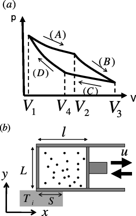
Figure 1: Schematic illustration of the model. (a) Pressure-volume ($p$-$V$) diagram of the quasistatic Carnot cycle for an ideal gas. (b) The piston moves at a finite constant speed $u$ and the thermalizing wall with the temperature $T_{i}$ ($i$=h, c) and the length $S$ is set on the left bottom of the cylinder only in the isothermal processes.

As time progresses, thermodynamic variables should draw a steady cycle independent of initial states. Fig. 2 shows the temperature-volume diagram for the steady cycle at $u=0.01$ and $u=0.001$, where $k_{\mathrm{B}}T$ is determined as the kinetic energy per particle, assuming the principle of equipartition. From this figure, we can see that in the isothermal expansion (compression) process the temperature approaches a steady value lower (higher) than $T_{\mathrm{h}}$ $(T_{\mathrm{c}})$ at $u=0.01$. This result can easily be understood: If a heat engine is working at a finite $u$, heat should flow into the system at a finite rate to maintain the steady cycle. Therefore, the finite difference of the temperatures between the system and the heat reservoir is necessary. The cycle for $u=0.001$ almost agrees with the quasistatic Carnot cycle of an ideal gas. This implies that our system of the hard-disc particles closely approximates an ideal gas system.

We have also calculated the efficiency $\eta=W_{\mathrm{total}}/Q_{\mathrm{h,total}}$ and the power $P=W_{\mathrm{total}}/{\tau}$, where $W_{\mathrm{total}}$ is the total work against the piston, $Q_{\mathrm{h,total}}$ is the total heat flowing into the system from the hot heat reservoir and $\tau$ is the total time for the simulation. Fig. 3 shows $\eta$ and $P$ at various $u$. We have found that the maximal power is realized at $u\approx 0.015$. The corresponding efficiency $\eta_{\mathrm{max}}$ (the efficiency at the maximal power) is about 0.18, which is close to the CA efficiency $\eta_{\mathrm{CA}}=0.163$.

Figure 2: Temperature-volume ($T$-$V$) diagram for the steady cycle at $u=0.01$ and $u=0.001$. The data were obtained by averaging over $1000$ cycles after transient $50$ cycles in the MD simulations. The solid line is the quasistatic Carnot cycle of an ideal gas. We can see that as $u$ becomes larger, the cycle obviously deviates from the quasistatic cycle.

Figure 3: $u$ dependence of the efficiency $\eta$ and the power $P$. The bold dots are the values calculated by the MD simulations and the solid line is the values calculated by solving Eq. (12) numerically. The MD data were obtained by the simulations for $100$-$2000$ cycles after $35$-$50$ transient cycles. In the limit of $u\to 0$, the Carnot efficiency ($\eta_{\mathrm{C}}=0.3$) is realized and $P$ vanishes.

3 Theoretical analysis

To explain the above MD data, we construct the theoretical model using the elementary molecular kinetic theory as below. We assume that even in a finite-time cycle, the gas relaxes to the uniform equilibrium state with a well-defined temperature $T$ very fast and the particle velocity $v$ is governed by Maxwell-Boltzmann distribution $f_{\mathrm{MB}}(\mbox{\boldmath$v$},T)$. We would like to derive the time-evolution equation of $T$. The energy $U$ of a two-dimensional equilibrium ideal gas is given by $U=Nk_{\mathrm{B}}T$. In the series of cycles, $U$ can be changed by two factors: particle collisions with the thermalizing wall and the piston. Our strategy to derive the time-evolution equation of $T$ is very simple: Counting the number of the particles colliding with the thermalizing wall and the piston and calculating the heat and the work from the difference between the kinetic energies before and after the collisions. Firstly, we consider the effect of the thermalizing wall. Since the number $n_{\mathrm{T}}$ of the particles with the velocity $v$ $(v_{y}<0)$ colliding with the thermalizing wall per unit time is given by $n_{\mathrm{T}}=f_{\mathrm{MB}}(\mbox{\boldmath$v$},T)S(-v_{y})N/V$, the total number $C$ of the particles colliding with the thermalizing wall per unit time is calculated as

$$C=\int_{-\infty}^{+\infty}dv_{x}\int_{-\infty}^{0}dv_{y}n_{\mathrm{T}}=\frac{SN}{2\pi V}\sqrt{\frac{2\pi k_{\mathrm{B}}T}{m}}.$$ (4)

The total energy of these colliding particles before the collisions is also given by

$$\int_{-\infty}^{+\infty}dv_{x}\int_{-\infty}^{0}dv_{y}n_{\mathrm{T}}\frac{m}{2}{\mbox{\boldmath$v$}}^{2}=\frac{3SNk_{\mathrm{B}}T}{4\pi V}\sqrt{\frac{2\pi k_{\mathrm{B}}T}{m}}.$$ (5)

Because the number of the reflecting particles is equal to the number of the colliding particles, the total energy of the particles after the collisions is calculated as

$$C\int_{0}^{+\infty}dv_{y}\int_{-\infty}^{\infty}dv_{x}f(\mbox{\boldmath$v$},T_{i})\frac{m}{2}\mbox{\boldmath$v$}^{2}$$

$$=\frac{3SNk_{\mathrm{B}}T_{i}}{4\pi V}\sqrt{\frac{2\pi k_{\mathrm{B}}T}{m}}$$ (6)

using Eq. (2). Therefore, the net energy transfer, namely the heat $q_{i}(t,T)$ flowing into the system per unit time in the isothermal processes ($i=\mathrm{h}$ in (A), $\mathrm{c}$ in (C)) is given by

$$q_{i}(t,T)=\frac{3SNk_{\mathrm{B}}(T_{i}-T)}{4\pi V(t)}\sqrt{\frac{2\pi k_{\mathrm{B}}T}{m}}.$$ (7)

Next, we derive the work against the piston by the colliding particles in the expansion processes. To calculate the number of particles colliding with the piston, we consider the velocity distribution $\tilde{f}_{\mathrm{MB}}(\tilde{v}_{x},v_{y},T)$ in the frame of the piston, where $\tilde{v}_{x}\equiv v_{x}-u$ and $\tilde{f}_{\mathrm{MB}}(\tilde{v}_{x},v_{y},T)\equiv f_{\mathrm{MB}}(\tilde{v}_{x}+u,v_{y},T)$ . The number $n_{\mathrm{M}}$ of the particles with the velocity $(\tilde{v}_{x},v_{y})$ colliding on the piston per unit time is $n_{\mathrm{M}}=\tilde{f}_{\mathrm{MB}}(\tilde{v}_{x},v_{y},T)L\tilde{v}_{x}N/V=\tilde{f}_{\mathrm{MB}}(\tilde{v}_{x},v_{y},T)\tilde{v}_{x}N/l$. Since a particle gives the work $2mu(v_{x}-u)=2mu\tilde{v}_{x}$ against the piston, the total work $w_{\mathrm{e}}(t,T)$ against the piston per unit time in the expansion processes becomes

$$w_{\mathrm{e}}(t,T) =\int_{-\infty}^{+\infty}dv_{y}\int_{0}^{+\infty}d\tilde{v}_{x}2mu\tilde{v}_{x}n_{\mathrm{M}}$$ (8)

$$=\frac{2muN}{l(t)}\biggl{\{}\frac{A^{2}T}{4}-Am^{3/2}\sqrt{\frac{T}{\pi}}u+\frac{u^{2}}{2}$$

$$-\int_{0}^{\frac{u}{A\sqrt{T}}}d{v_{x}}\left(A\sqrt{T}{v_{x}}-u\right)^{2}\frac{\mathrm{e}^{-{v_{x}}^{2}}}{\sqrt{\pi}}\biggr{\}},$$

where $A\equiv\sqrt{{2k_{\mathrm{B}}}/{m}}$. The work $w_{\mathrm{c}}(t,T)$ for the unit time in the compression processes is also obtained by changing $u\to-u$ in Eq. (8).

By the energy conservation law, the time evolution of $T$ for each of four processes (A)-(D) is given by

$$\begin{array}[]{c c}(\mathrm{A}):Nk_{\mathrm{B}}\displaystyle{\frac{dT}{dt}}=q_{\mathrm{h}}-w_{\mathrm{e}},&(\mathrm{B}):Nk_{\mathrm{B}}\displaystyle{\frac{dT}{dt}}=-w_{\mathrm{e}},\\ \\ (\mathrm{C}):Nk_{\mathrm{B}}\displaystyle{\frac{dT}{dt}}=q_{\mathrm{c}}-w_{\mathrm{c}},&(\mathrm{D}):Nk_{\mathrm{B}}\displaystyle{\frac{dT}{dt}}=-w_{\mathrm{c}}.\end{array}$$ (12)

Here, we have numerically solved the above Eq. (12) for the entire cycle. By using the final temperature of each process as the initial temperature of the next process repeatedly, we can obtain the steady cycle of this heat engine. After reaching the steady cycle, we numerically calculate the efficiency $\eta(u)={W(u)}/{Q_{\mathrm{h}}(u)}$ and the power $P(u)={W(u)u}/(2(l_{3}-l_{1}))$, where $Q_{\mathrm{h}}(u)$ is the heat transfer from the hot reservoir to the system, $W(u)$ is the work output and ${2(l_{3}-l_{1})}/{u}$ is the time for one steady cycle. In Fig. 3, we plot the $u$ dependence of $\eta$ and $P$ at the same parameters as in the MD simulations. From this figure, we can see that the correspondence between the MD data and the line calculated by solving Eq. (12) numerically is established qualitatively. This implies that our assumption of fast relaxation to the equilibrium state is not so bad .

Figure 4: The efficiency at the maximal power $\eta_{\mathrm{max}}$. The bold dots are the MD data, the solid line is the theoretical line calculated by solving Eq. (12) numerically, the dashed line is the the analytic expression Eq. (21) and the dotted line is the CA efficiency Eq. (1).

In Fig. 4, we compare the efficiency at the maximal power $\eta_{\mathrm{max}}=\eta(u_{\mathrm{max}})$, where $u_{\mathrm{max}}$ is the speed giving the maximal power, with the CA efficiency Eq. (1) at $T_{\mathrm{h}}=1$ and various $T_{\mathrm{c}}$. We have found that our $\eta_{\mathrm{max}}$ does not always agree with $\eta_{\mathrm{CA}}$ but tends to approach $\eta_{\mathrm{CA}}$ as $T_{\mathrm{c}}\to T_{\mathrm{h}}$ for both of the MD data and the numerical line. We have confirmed that this $\eta_{\mathrm{max}}$ behavior is common to the systems with various parameters $V_{1},V_{2},S,$ etc., though the data are not shown here. To explain this $\eta_{\mathrm{max}}$ behavior, we try to obtain the analytic form of $\eta_{\mathrm{max}}$ by solving the evolution equation of $T$ in the following.

As seen in Fig. 2, we can expect that $T$ approaches a steady value $T_{\mathrm{h}}^{\mathrm{st}}$ in the isothermal expansion process (A). Then, $T_{\mathrm{h}}^{\mathrm{st}}$ is obtained as a solution of the equation $dT/dt=0$ in Eq. (12A). Because $T_{\mathrm{h}}^{\mathrm{st}}=T_{\mathrm{h}}$ is realized in the quasistatic limit $u\to 0$, we can expand $T_{\mathrm{h}}^{\mathrm{st}}$ by $u$ as $T_{\mathrm{h}}^{\mathrm{st}}=T_{\mathrm{h}}+T_{\mathrm{h}}^{(1)}u+T_{\mathrm{h}}^{(2)}u^{2}+{\cal O}(u^{3})$. Substituting $T_{\mathrm{h}}^{\mathrm{st}}$ into Eq. (12A), we can determine $T_{\mathrm{h}}^{(1)}$ and $T_{\mathrm{h}}^{(2)}$ and obtain $T_{\mathrm{h}}^{\mathrm{st}}$ up to ${\cal O}(u^{2})$ as

$$T_{\mathrm{h}}^{\mathrm{st}}=T_{\mathrm{h}}-\frac{4Lu}{3S}\biggl{\{}\frac{\sqrt{\pi T_{\mathrm{h}}}}{A}+\frac{mu}{k_{\mathrm{B}}}\left(2+\frac{\pi L}{3S}\right)\biggl{\}}.$$ (13)

If we assume that the relaxation to $T_{\mathrm{h}}^{\mathrm{st}}$ is very fast, the heat flowing into the system during $T(t)=T_{\mathrm{h}}^{\mathrm{st}}$ is given by

$$Q_{\mathrm{h}}^{\mathrm{st}} =\int_{0}^{(l_{2}-l_{1})/u}q_{\mathrm{h}}(t,T_{\mathrm{h}}^{\mathrm{st}})\ dt$$ (14)

$$=Q_{\mathrm{h}}^{\mathrm{qs}}-2mNA\sqrt{T_{\mathrm{h}}\pi}\left(\frac{1}{\pi}+\frac{L}{3S}\right)u\ln\frac{V_{2}}{V_{1}},$$

using Eq. (7), where the quasistatic heat for ideal gas in the isothermal expansion process is defined as $Q_{\mathrm{h}}^{\mathrm{qs}}\equiv Nk_{\mathrm{B}}T_{\mathrm{h}}\ln(V_{2}/V_{1})$. Note that $Q_{\mathrm{h}}^{\mathrm{st}}\to Q_{\mathrm{h}}^{\mathrm{qs}}$ when we consider the quasistatic limit $u\to 0$. $T_{\mathrm{c}}^{\mathrm{st}}$ and $Q_{\mathrm{c}}^{\mathrm{st}}$ of the isothermal compression process (C) can be obtained by replacing $T_{\mathrm{h}},u,V_{1}$ and $V_{2}$ in Eqs. (13) and (14) with $T_{\mathrm{c}},-u,V_{3}$ and $V_{4}$, respectively. Firstly, we try to calculate $\eta_{\mathrm{max}}$ by using $Q_{\mathrm{h}}^{\mathrm{st}}$ and $Q_{\mathrm{c}}^{\mathrm{st}}$ above. By defining the work of one cycle $W$ as $W=Q_{\mathrm{h}}^{\mathrm{st}}+Q_{\mathrm{c}}^{\mathrm{st}}$, we can calculate the efficiency $\eta=W/Q_{\mathrm{h}}^{\mathrm{st}}$ and the power $P={Wu}/(2(l_{3}-l_{1}))$. The maximal power is realized at $u=u_{\mathrm{max}}$ defined as a solution of $\partial P/\partial u=0$. Since $u_{\mathrm{max}}$ is given by

$$u_{\mathrm{max}}=\frac{k_{\mathrm{B}}(T_{\mathrm{h}}-T_{\mathrm{c}})}{4m(\frac{1}{\pi}+\frac{L}{3S})\sqrt{\frac{2\pi k_{\mathrm{B}}}{m}}(\sqrt{T_{\mathrm{h}}}+\sqrt{T_{\mathrm{c}}})},$$ (15)

$Q_{\mathrm{h}}^{\mathrm{st}}$ and $W$ at $u_{\mathrm{max}}$ are obtained as

$$Q_{\mathrm{h}}^{\mathrm{st}}(u_{\mathrm{max}}) =\frac{N}{2}k_{\mathrm{B}}\sqrt{T_{\mathrm{h}}}(\sqrt{T_{\mathrm{h}}}+\sqrt{T_{\mathrm{c}}})\ln\frac{V_{2}}{V_{1}},$$ (16)

$$W(u_{\mathrm{max}}) =\frac{N}{2}k_{\mathrm{B}}(T_{\mathrm{h}}-T_{\mathrm{c}})\ln\frac{V_{2}}{V_{1}}.$$ (17)

Moreover, $\eta_{\mathrm{max}}\equiv\eta(u_{\mathrm{max}})$ is calculated as

$$\eta_{\mathrm{max}}=\frac{W(u_{\mathrm{max}})}{Q_{\mathrm{h}}^{\mathrm{st}}(u_{\mathrm{max}})}=1-\sqrt{\frac{T_{\mathrm{c}}}{T_{\mathrm{h}}}}.$$ (18)

This is equal to the CA efficiency Eq. (1) though we neglect ${\cal O}(u^{2})$ in the calculation of $Q_{\mathrm{h}}^{\mathrm{st}}$ and $Q_{\mathrm{c}}^{\mathrm{st}}$. Therefore, we may regard that this result gives a natural and microscopic foundation of the original derivation of the CA efficiency Eq. (1).

As seen in Fig. 4, however, the CA efficiency deviates from the MD data and the numerically calculated line. This is because there exists the heat transfer other than $Q_{\mathrm{h}}^{\mathrm{st}}$ and $Q_{\mathrm{c}}^{\mathrm{st}}$, which may be missed in the original derivation of Eq. (1) [1]. As seen in Fig. 2, the initial temperatures of isothermal processes are different from the steady values. This implies the existence of the additional heat transfer $Q_{\mathrm{h}}^{\mathrm{add}}$ and $Q_{\mathrm{c}}^{\mathrm{add}}$ during the fast relaxation to the steady temperatures. Next, we repeat the similar derivation of Eq. (18) by considering the effect of these additional heat transfers $Q_{\mathrm{h}}^{\mathrm{add}}$ and $Q_{\mathrm{c}}^{\mathrm{add}}$. We define the total heat as $Q_{\mathrm{h}}=Q_{\mathrm{h}}^{\mathrm{st}}+Q_{\mathrm{h}}^{\mathrm{add}}$ and $Q_{\mathrm{c}}=Q_{\mathrm{c}}^{\mathrm{st}}+Q_{\mathrm{c}}^{\mathrm{add}}$. Since we assume that the relaxation to the steady temperature is very fast, we can approximate the additional heat transfers as $Q_{\mathrm{h}}^{\mathrm{add}}=Nk_{\mathrm{B}}(T_{\mathrm{h}}^{\mathrm{st}}-\tilde{T_{\mathrm{h}}})$ and $Q_{\mathrm{c}}^{\mathrm{add}}=Nk_{\mathrm{B}}(T_{\mathrm{c}}^{\mathrm{st}}-\tilde{T_{\mathrm{c}}})$, where $\tilde{T_{\mathrm{h}}}$ and $\tilde{T_{\mathrm{c}}}$ are the initial temperatures of the isothermal processes (A) and (C), respectively. If we assume that adiabatic processes satisfy the relations $\tilde{T_{\mathrm{h}}}=({V_{4}}/{V_{1}})T_{\mathrm{c}}^{\mathrm{st}}$ and $\tilde{T_{\mathrm{c}}}=({V_{2}}/{V_{3}})T_{\mathrm{h}}^{\mathrm{st}}$ which are the same as in the quasistatic case, we can obtain

$$Q_{\mathrm{h}}^{\mathrm{add}}=-Nk_{\mathrm{B}}\frac{4L\sqrt{\pi T_{\mathrm{h}}}}{3SA}\left(1+\sqrt{\frac{T_{\mathrm{h}}}{T_{\mathrm{c}}}}\right)u$$ (19)

up to ${\cal O}(u)$. $Q_{\mathrm{c}}^{\mathrm{add}}$ is given by changing $T_{\mathrm{h}}\leftrightarrow T_{\mathrm{c}}$ and $u\to-u$ in Eq. (19). The work of one cycle $W$ is defined as $W=Q_{\mathrm{h}}^{\mathrm{st}}+Q_{\mathrm{c}}^{\mathrm{st}}+Q_{\mathrm{h}}^{\mathrm{add}}+Q_{\mathrm{c}}^{\mathrm{add}}$. By defining $u_{\mathrm{max}}$ as a solution of $\partial P/\partial u=0$, we can obtain

$$u_{\mathrm{max}} =\frac{k_{\mathrm{B}}(T_{\mathrm{h}}-T_{\mathrm{c}})}{\sqrt{\pi}}\Biggl{\{}4mA\left(\frac{L}{3S}+\frac{1}{\pi}\right)$$ (20)

$$\times(\sqrt{T_{\mathrm{h}}}+\sqrt{T_{\mathrm{c}}})\ln\frac{V_{2}}{V_{1}}+\frac{8Lk_{\mathrm{B}}}{3SA\sqrt{T_{\mathrm{h}}}}$$

$$\times\left(T_{\mathrm{h}}-T_{\mathrm{c}}\right)\left(1+\sqrt{\frac{T_{\mathrm{h}}}{T_{\mathrm{c}}}}\right)\Biggr{\}}^{-1}\ln\frac{V_{2}}{V_{1}},$$

$$\eta_{\mathrm{max}} \equiv\eta(u_{\mathrm{max}})=\frac{\frac{N}{2}k_{\mathrm{B}}(T_{\mathrm{h}}-T_{\mathrm{c}})\ln\frac{V_{2}}{V_{1}}}{Q_{\mathrm{h}}^{\mathrm{st}}(u_{\mathrm{max}})+Q_{\mathrm{h}}^{\mathrm{add}}(u_{\mathrm{max}})}.$$ (21)

From Fig. 4, we can see that Eq. (21) agrees with the MD data and the numerically calculated result very well due to the effect of the additional heat $Q_{\mathrm{h}}^{\mathrm{add}}$ and $Q_{\mathrm{c}}^{\mathrm{add}}$. To obtain the efficiency in the $T_{\mathrm{c}}\to T_{\mathrm{h}}$ limit, we set $T_{\mathrm{c}}=T_{\mathrm{h}}-\Delta T$ $(\Delta T\ll 1)$. Then, $\eta_{\mathrm{max}}$ is given by $\eta_{\mathrm{max}}={\Delta T}/(2T_{\mathrm{h}})+{\cal O}(\Delta T^{2})$ which is the same as the CA efficiency up to $\Delta T$ order. This result explains why our $\eta_{\mathrm{max}}$ approaches $\eta_{\mathrm{CA}}$ when $T_{\mathrm{c}}\to T_{\mathrm{h}}$. Very recently, similar $\eta_{\mathrm{max}}$ behavior has been observed also in the other types of the heat engines [13, 14]. In the equilibrium limit of $T_{\mathrm{c}}\to T_{\mathrm{h}}$, the system may be regarded as being in the linear response regime. Therefore, our result is consistent with the CA efficiency proved by using the linear response theory [6].

4 Summary

In this paper, we have studied the efficiency at the maximal power $\eta_{\mathrm{max}}$ of a finite-time Carnot cycle of a weakly interacting gas which we can regard as a nearly ideal gas. Our model is a natural extension of the quasistatic Carnot cycle and has a piston moving back and forth at a constant speed $u$ in the cylinder. We have used this $u$ as a unique parameter to maximize the power. Since $u$ is easily controllable, this model seems more natural than the original Curzon-Ahlborn’s model [1]. We have performed numerical experiments of this model by means of MD simulations to verify the validity of the Curzon-Ahlborn (CA) efficiency $\eta_{\mathrm{CA}}$ for the first time and have found that our $\eta_{\mathrm{max}}$ does not always agree with $\eta_{\mathrm{CA}}$, but approaches $\eta_{\mathrm{CA}}$ in the limit of $T_{\mathrm{c}}\to T_{\mathrm{h}}$. Our molecular kinetic analysis can explain the above facts theoretically by using only elementary arithmetic. Especially, we have revealed that the difference between $\eta_{\mathrm{CA}}$ and our $\eta_{\mathrm{max}}$ is due to the additional heat transfers which may be missed in the original derivation of $\eta_{\mathrm{CA}}$ [1]. Though it is restricted in the equilibrium limit of $T_{\mathrm{c}}\to T_{\mathrm{h}}$, these results strongly support the validity of the CA efficiency from both of the experimental and theoretical points of view. We expect that our analysis in this paper will shed light on the microscopic aspects of the finite-time extension of thermodynamics.

- [1] \NameCurzon F. L. Ahlborn B. \REVIEWAm. J. Phys.43197522.
- [2] \NameCallen H. \BookThermodynamics and an Introduction to Thermostatistics, 2nd edition \PublWiley, New York \Year1985, Chapt. 4.
- [3] \NameNovikov I. I. \REVIEWJ. Nucl. Energy7, issues No. 1-21958125.
- [4] \NameBejan A. \REVIEWJ. Appl. Phys.7919961191.
- [5] \NameLandsberg P. T. Leff H. \REVIEWJ. Phys.2219894019.
- [6] \Namevan den Broeck C. \REVIEWPhys. Rev. Lett.952005190602.
- [7] \NameGomez-Marin A. Sancho J. M. \REVIEWPhys. Rev. E.742006062102.
- [8] \NameJiménez de Cisneros B. Hernández A. C. \REVIEWPhys. Rev. Lett.982007130602.
- [9] \NameKosloff R. \REVIEWJ. Chem. Phys.8019841625.
- [10] \NameAlder B. J. Wainright T. E. \REVIEWJ. Chem. Phys.2719571208.
- [11] \NameYuge T., Ito N. Shimizu A. \REVIEWJ. Phys. Soc. Jpn.7420051895.
- [12] \NameHondou T. \REVIEWEurophys. Lett.80200750001.
- [13] \NameSchmiedl T. Seifert U. \REVIEWEurophys. Lett.81200820003.
- [14] \NameAllahverdyan A. E., Johal R. S. Mahler G. \REVIEWPhys. Rev. E.772008041118.