Plankton blooms in vortices: The role of biological and hydrodynamic timescales.

Abstract

We study the interplay of hydrodynamic mesoscale structures and the growth of plankton in the wake of an island, and its interaction with a coastal upwelling. Our focus is on a mechanism for the emergence of localized plankton blooms in vortices. Using a coupled system of a kinematic flow mimicking the mesoscale structures behind the island and a simple three component model for the marine ecosystem, we show that the long residence times of nutrients and plankton in the vicinity of the island and the confinement of plankton within vortices are key factors for the appearance of localized plankton blooms.

1 Introduction

The interplay between hydrodynamic motion and the distribution of marine organisms like phytoplankton and zooplankton is a major challenge recently addressed in numerous studies (Mann and Lazier, 1991; Denman and Gargett, 1995; Abraham, 1998; Peters and Marrasé, 2000; Károlyi et al., 2000; López et al., 2001a, b; Martin et al., 2002; Martin, 2003; Sandulescu et al., 2007b).

The growth of phytoplankton in the world’s oceans depends strongly on the availability of nutrients. Thus, one of the essential factors controlling the primary production is the vertical transport of nutrients. Coastal upwelling is one of the most important mechanisms of this type. It usually occurs when wind-driven currents, in combination with the Coriolis force, produces Ekman transport, by which surface waters are driven away from the coast and are replaced by nutrient-rich deep waters. Due to this nutrient enrichment, primary production in these areas is strongly boosted, giving rise also to an increase of zooplankton and fish populations.

On the other side, the interplay between plankton dynamics and horizontal transport, mixing and stirring has been investigated in several studies recently (Abraham, 1998; López et al., 2001b; Hernández-García et al., 2002, 2003; Martin, 2003). Horizontal stirring by mesoscale structures like vortices and jets redistributes plankton and nutrients and may enhance primary production (Martin et al., 2002; Hernández-García and López, 2004). Horizontal transport can also initiate phytoplankton blooms and affects competition and coexistence of different plankton species (Károlyi et al., 2000; Bracco et al., 2000).

Vertical upwelling in connection with strong mesoscale activity occurs in several places on Earth. One of these regions is the Atlantic ocean area close to the northwestern African coast, near the Canary archipelago. The main water current in this area flows from the Northeast towards the Canary islands, in which wake strong mesoscale hydrodynamic activity is observed (Arístegui et al., 1997). The interaction between the vortices emerging in the wake of the Canary islands and the Ekman flow seems to be essential for the observed enhancement of biological production in the open southern Atlantic ocean close to the Canary islands (Arístegui et al., 2004). The aim of this paper is to study the interplay between the redistribution of plankton by the vortices and the primary production. In particular we focus on the role of residence times of plankton particles in the wake of the island. Though we believe that our study is relevant for different areas in the world, we focus on the situation around the Canary archipelago to be specific.

In this work we consider the coupling of the kinematic flow introduced in (Sandulescu et al., 2006a) to a simplified model of plankton dynamics with three trophic levels, and study the impact of the underlying hydrodynamic activity and the upwelling of nutrients on primary production in different areas of the wake. In this setup vortices have been reported to play an essential role in the enhancement of primary production (Sandulescu et al., 2007b). Our main objective here is to analyze this mechanism in detail and show that the extended residence times of plankton within vortices are responsible for the observation of localized algal blooms in them.

The organization of the paper is as follows. In section 2 we present the general framework of our system, indicating the hydrodynamical and the biological model, as well as their coupling. Our main analysis is devoted to the mechanism of the appearance of a localized plankton bloom within a vortex (Sec. 3). We study the residence times of plankton within vortices and in the neighborhood of the island. Additionally we clarify the role of the chaotic saddle embedded in the flow in the wake of the island. Finally we summarize and discuss our results in Sec. 4.

2 General framework: velocity field, plankton model and boundary conditions

Our system consists of a hydrodynamic flow with an embedded obstacle and vortices in its wake. The model contains also a current perpendicular to the main flow that models an Ekman flow coming from the coast, and a nutrient-rich region at a distance from the obstacle simulating a coastal upwelling zone. A sketch of the model is shown in Fig. 1. With this simplified geometry we mimic the essential features of the hydrodynamic flow in the Canaries (note that the whole Canary archipelago is approximated by one cylindrical island). In particular, in the wake of the obstacle strong mesoscale activity is observed in the form of a periodic detachment of vortices, which then travel in the main flow direction.

We use the kinematic model first developed by Jung et al. (1993), which we modified by the introduction of the Ekman flow (Sandulescu et al., 2006a). This model is coupled to a simple population dynamics which features the interaction of nutrients $N$, phytoplankton $P$ and zooplankton $Z$. The next two subsections are devoted to the introduction of the hydrodynamic as well as the biological model before discussing the results of coupling both models to study the feedback between hydrodynamics and phytoplankton growth.

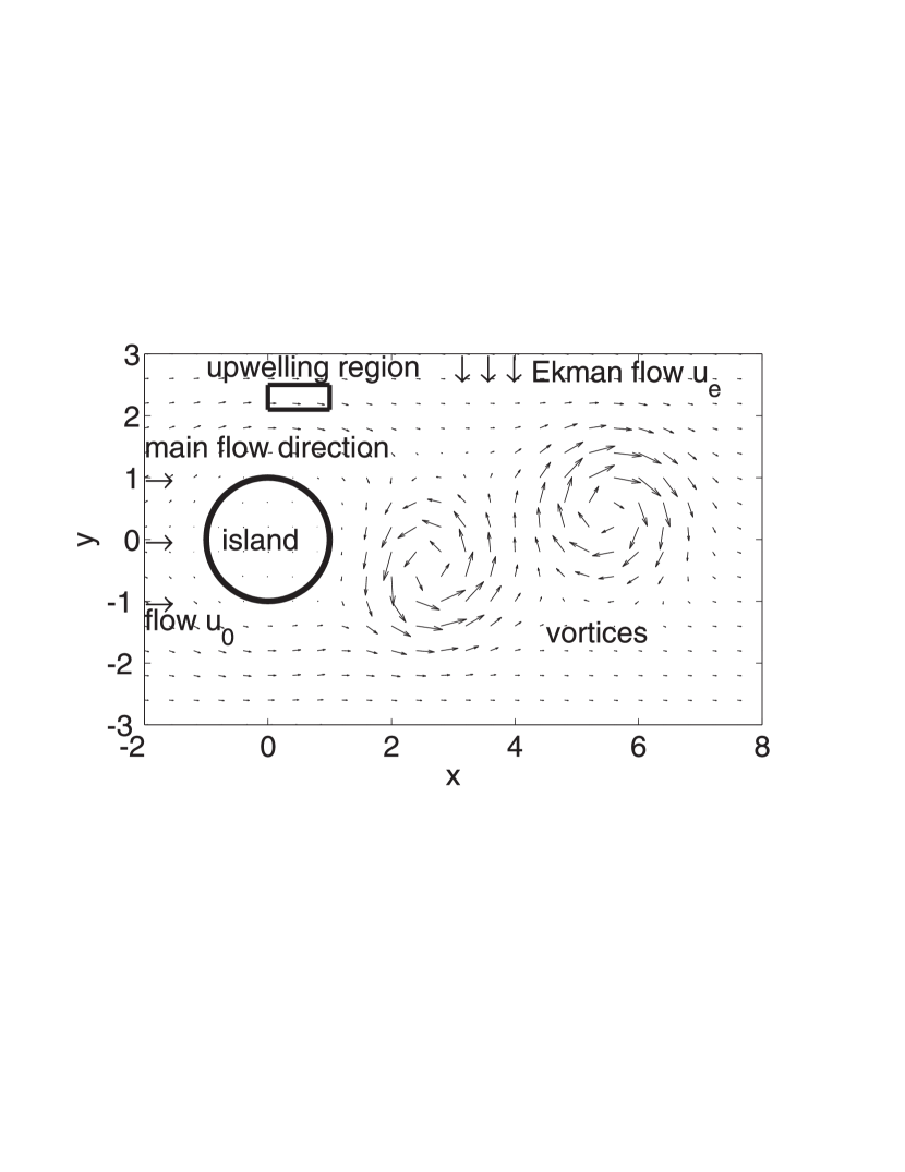
Figure 1: The simplified island wake model setup.

2.1 The hydrodynamic model

We now introduce the velocity field. Details can be found in (Sandulescu et al., 2006a). The setup of our hydrodynamic model is based on a horizontal flow pattern. As Fig. 1 shows the main current runs from left to right along the horizontal $x$ direction. The center of the cylinder is placed at the origin of the coordinate system. We consider a two-dimensional velocity field which can be computed analytically from a stream function $\Psi$. The velocity components in $x$- and $y$-direction and the equations of motion of fluid elements are:

$$\dot{x} = v_{x}(x,y,t)=\frac{\partial}{\partial y}\Psi(x,y,t),$$

$$\dot{y} = v_{y}(x,y,t)=-\frac{\partial}{\partial x}\Psi(x,y,t).$$ (1)

The stream function is given by the product of two terms (Jung et al., 1993):

$$\Psi(x,y,t)=f(x,y)g(x,y,t).$$ (2)

The first factor $f(x,y)$ ensures the correct boundary conditions at the cylinder, $f(x,y)=1-\exp\left[-a\left(\sqrt{x^{2}+y^{2}}-1\right)^{2}\right]$. The second factor $g(x,y,t)$ models the background flow, the vortices in the wake, and the Ekman flow $g(x,y)=-wh_{1}(t)g_{1}(x,y,t)+wh_{2}(t)g_{2}(x,y,t)+u_{0}s(x,y)y+u_{E}\Theta(x-1)x$. The vortices in the wake are of opposite sign but their maximal vortex strengths are equal and denoted by $w$, and its shape is described by the functions $g_{i}$ (see details in Sandulescu et al. (2006a)). The characteristic linear size of the vortices is given by $\kappa_{0}^{-1/2}$ and the characteristic ratio between the elongation of the vortices in the $x$ and $y$ direction is given by $\alpha$. The vortex centers move along the $x$ direction according to $x_{1}(t)=1+L\left(t/T_{c}\ {\rm mod}\ 1\right)$ and $x_{2}(t)=x_{1}(t-T_{c}/2)$, and at values of $y_{i}(t)$ described below. Each vortex travels along the $x$ direction for a time $T_{c}$ and disappears. The background flow moves in the positive horizontal direction with a speed $u_{0}$. The factor $s(x,y)$ describes the shielding of the background flow by the cylinder in a phenomenological manner, using the same elongation factor $\alpha$ as for the vortices. The Ekman drift, which is intended to model the flow from the coast towards the ocean interior, is introduced by considering an additional velocity of constant strength $u_{E}$ in the $y$ direction acting only at $x$ coordinates larger than $1$, i.e. just behind the island. This corresponds to a stream crossing the vortex street towards negative $y$ values beyond the cylinder.

Real oceanic flows are never perfectly periodic. Therefore we use a non-periodic version of the kinematic flow just presented. Non-periodicity is achieved by adding some randomness to the vortex trajectories. Instead of moving along straight horizontal lines, $y_{1}(t)=y_{0}$, $y_{2}(t)=-y_{0}$ ($y_{0}$ constant), the vertical coordinates of the vortices move according to $y_{1}(t)=y_{0}+\epsilon\xi(t)$, and $y_{2}(t)=-y_{1}(t)$, where, at each time, $\xi(t)$ is a uniform random number in the range $[-1,1]$, and $\epsilon$ is the noise strength.

The parameters of the model are chosen in such a way that they represent properly the geophysical features of the Canary zone. These values are given in Table 1. To make the model dimensionless we measure all lengths in units of the island radius $r=25$ km and all times in units of the period $T_{c}=30$ days. For a discussion of all parameters we refer to (Sandulescu et al., 2006a), where the adaptation of the model to the situation around the Canary islands is discussed in detail.

Table 1: List of parameters used in the hydrodynamical model

parameter	value	dimensionless value
$r$	25 km	1
$u_{0}$	0.18 m/s	18.66
$\kappa_{0}^{-1/2}$	25 km	1
$\alpha$	1	1
$w$	$\approx 55\times 10^{3}\ m^{2}/s$	200
$T_{c}$	30 days	1
$L$	6r = 150 km	6
$a^{-1/2}$	25 km	1
$u_{E}$	0.02 m/s	2
$y_{0}$	$r/2$=12.5 km	0.5
$\epsilon$	6.25 km	0.5

2.2 The biological model

One can find in the literature a large variety of different models used to analyse the dynamics of marine ecosystems. Their complexity ranges from simple ones with only a few interacting components (Steele and Henderson, 1981, 1992) to large comprehensive ones (Baretta et al., 1997). We use a system which is based on a three component model developed by Steele and Henderson (1992) and later modified by (Edwards and Brindley, 1996) and (Oschlies and Garçon, 1999).

The model describes the interaction of three species in a trophic chain, namely nutrients $N$, phytoplankton $P$ and zooplankton $Z$, whose concentrations evolve in time according to the following dynamics:

$$\frac{dN}{dt}=~{}F_{N}~{} = \Phi_{N}-\beta\frac{N}{k_{N}+N}P+$$

$$+ \mu_{N}\left((1-\gamma)\frac{\alpha\eta P^{2}}{\alpha+\eta P^{2}}Z+\mu_{P}P+\mu_{Z}Z^{2}\right)$$

$$\frac{dP}{dt}=~{}F_{P}~{} = \beta\frac{N}{k_{N}+N}P-\frac{\alpha\eta P^{2}}{\alpha+\eta P^{2}}Z-\mu_{P}P$$

$$\frac{dZ}{dt}=~{}F_{Z}~{} = \gamma\frac{\alpha\eta P^{2}}{\alpha+\eta P^{2}}Z-\mu_{Z}Z^{2}$$ (3)

Let us now briefly discuss the meaning of the different terms (cf. Oschlies and Garçon (1999) and Pasquero et al. (2004) for details): the dynamics of the nutrients is determined by nutrient supply due to vertical mixing, recycling by bacteria and consumption by phytoplankton. Vertical mixing which brings nutrients from lower layers of the ocean into the mixed layer is parameterized in the biological model, since the hydrodynamical part considers only horizontal transport of nutrients. For the vertical mixing we assume $N_{0}$ as a constant nutrient concentration below the mixed layer. Thus the mixing term reads:

$$\Phi_{N}=S(x,y)(N_{0}-N),$$ (4)

where the function $S$ determines the strength of the upwelling and will be discussed in more detail below. The nutrients are consumed by phytoplankton with a saturation characteristics described by a Holling type II functional response. The recycling by bacteria is modelled by the last three terms in the bracket. A part of all dead organic matter as well as the exudation of zooplankton is degraded by bacteria, though the dynamics of the bacteria themselves is not included in the model. The phytoplankton grows upon the uptake of nutrients, but its concentration is diminished by zooplankton (grazing term) and due to natural mortality. Grazing, modelled by a Holling type III function, enters also as a growth term for the zooplankton dynamics multiplied by a factor $\gamma$ taking into account that only a part of the food is converted into biomass of the zooplankton, while the other part $(1-\gamma)$ goes to recycling. The natural mortality of zooplankton is assumed to be quadratic because this term does not only model natural mortality but also the existence of higher predators which are not explicitly considered (Edwards and Bees, 2001). The parameters used are taken from (Pasquero et al., 2004) as presented in Table 2. Although appropriate for open ocean, they would provide estimates for biological properties in the Atlantic not too close to the coast. To obtain dimensionless quantities convenient for the numerics, space is measured in units of $r$, time in units of $T_{c}$ and mass in units of $10^{12}$ mmol N.

Table 2: List of parameters used in the biological model

parameter	value	dimensionless value
$\beta$	0.66 day-1	19.8
$\eta$	1.0 (mmol N m${}^{-3})^{-2}$ day-1	0.12288
$\gamma$	0.75	0.75
$a$	2.0 day-1	60
$S_{l}$	0.00648 day-1 (nutrient poor)	0.1944
$S_{h}$	0.648 day-1 (nutrient rich)	19.44
$k_{N}$	0.5 mmol N m-3	7.8125
$\mu_{N}$	0.2	0.2
$\mu_{P}$	0.03 day -1	0.9
$\mu_{Z}$	0.2 (mmol N m${}^{-3})^{-1}$ day-1	0.384
$N_{0}$	8.0 mmol N m-3	125

The primary production is defined as the growth term in the phytoplankton dynamics:

$$PP=\beta\frac{N}{k_{N}+N}P$$ (5)

The function $S$, measuring the strength of vertical mixing in this model is a crucial quantity for the coupling between the hydrodynamical and the biological model, because it quantifies the local nutrient supply. As shown in Fig. 1 we assume that there exists an upwelling zone which is located in a small rectangular region on one side of the island. According to this assumption, we assign two different values to the parameter $S(x,y)$. In the upwelling zone there is a strong vertical mixing leading to nutrient rich waters in the mixed layer. There we assume $S(x,y)=S_{h}=0.648$ day^-1, while in all the surrounding waters upwelling is much lower so that we assign $S(x,y)=S_{l}=0.00648$ day^-1 which is a hundred times lower.

The dynamics of this model is different depending on the choice of parameters. The long-term behavior can be either stationary with constant concentrations of $N$, $P$ and $Z$ or oscillatory. We refer for more details to Edwards and Brindley (1996) and Pasquero et al. (2004). We use a parameter set where the system possesses a stable steady-state. Using the parameter values from Table 2 and setting the vertical mixing $S=S_{l}=0.00648$ day^-1 we obtain as a steady state $N_{amb}=0.185$, $P_{amb}=0.355$ and $Z=Z_{amb}=0.444$ mmol N m^-3. In this nutrient poor region the ambient primary production is $PP_{amb}=0.0633$ mmol N m^-3 day^-1.

2.3 The coupled model

The coupling of the biology and the hydrodynamics yields a system of advection-reaction-diffusion equations. Thus the complete model is given by the following system of partial differential equations:

$$\frac{\partial N}{\partial t}+{\vec{v}}\cdot\nabla N = F_{N}+D\nabla^{2}N,$$

$$\frac{\partial P}{\partial t}+{\vec{v}}\cdot\nabla P = F_{P}+D\nabla^{2}P,$$

$$\frac{\partial Z}{\partial t}+{\vec{v}}\cdot\nabla Z = F_{Z}+D\nabla^{2}Z,$$ (6)

with the biological interactions $F_{N}$, $F_{P}$, and $F_{Z}$ from Eq. (3), and the velocity field ${\vec{v}}(x,y,t)$ from Eqs. (1) and (2). The diffusion terms take into account the small scale turbulence with eddy diffusivity $D$. We take $D\approx 10m^{2}/s$, as corresponding to the Okubo estimation of eddy diffusivity at scales of about 10 km (Okubo, 1971), the scales which begin to be missed in our large scale streamfunction. This advection-reaction-diffusion system is solved numerically by means of the method explained in Appendix A. As we are studying an open flow, the inflow conditions into the left part of the computational domain have to be specified to complete the model definition. Depending on the choice of the inflow concentrations we observe different behavior. A detailed analysis can be found in (Sandulescu et al., 2007b), here we only recall the main results which are the basis of the analysis we present here. We have studied two essentially different inflow conditions:

1. In the first one fluid parcels enter the computational domain with the ambient concentrations $N_{amb}$, $P_{amb}$, and $Z_{amb}$ corresponding to the steady-state for $S=S_{l}$. In this case the exterior of the computational domain has the same properties as the part of the domain without upwelling.

2. In the second one fluid parcels transported by the main flow enter the domain from the left with a very small content of nutrients and plankton, corresponding to a biologically very poor open ocean outside the considered domain. In particular we take $N_{L}=0.01\times N_{amb}$, $P_{L}=0.01\times P_{amb}$ and $Z_{L}=0.01\times Z_{amb}$, leading to very low primary production in the inflow water $PP_{L}=8.6\times 10^{-6}$ mmol N m^-3 day^-1. Since those concentrations are very low, we take into account that fluctuations may be important by adding to each of the concentrations $(N_{L},P_{L},Z_{L})$ some Gaussian noise term (cf. Sandulescu et al. (2007b) for details).

The two inflow concentrations yield different behavior as shown in Fig. 2. In the first case we observe high biological activity connected with a high primary production in the area outside vortices. Namely, this is the area of the nutrient plumes advected from the upwelling region (Fig. 2 left column). By contrast, in the second inflow case (Fig. 2 right column) we obtain a high phytoplankton concentration within the vortices. It turns out that here the vortices act as incubators for primary production leading to localized plankton blooms. In the first inflow case the behavior is easy to understand since due to higher nutrient concentrations in the upwelling region and its neighborhood a high growth of phytoplankton is expected. The response on the upwelling of nutrients in the second case is less obvious. Therefore the main objective of this paper is to find out the mechanism of the localized plankton blooms. In the rest of this work we consider only the situation that the concentrations at inflow are at their low values $N_{L},P_{L},Z_{L}$.

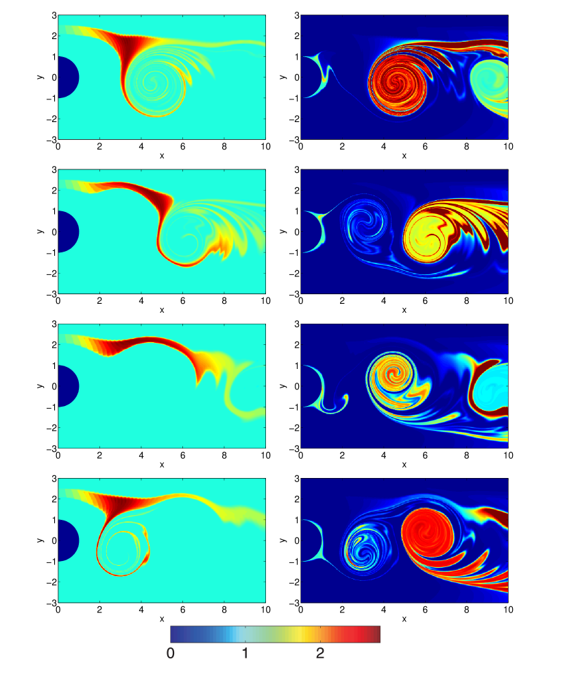
Figure 2: The concentration of phytoplankton (normalized with the steady state concentration, $P_{amb}$) for inflow at ambient concentrations (left) and for low inflow concentrations (right). Snapshots taken at $t/T_{c}=4.1,4.35,4.6,4.85$.

3 The mechanism of emergence of localized plankton blooms

After specifying the complete model and its dynamics we now investigate the behavior of the coupled biological and hydrodynamical system from different perspectives to clarify the mechanism of localized enhancement of phytoplankton and primary production connected to vortices. Firstly we study the biological model alone to understand the interplay between the three biological components $N,P$ and $Z$ leading to a sharp increase of phytonplankton for some time interval. This study yields a certain biological time scale for the growth of plankton which we compare in a second step to the hydrodyamical time scale obtained from the investigations of residence times in vortices. Thirdly we discuss the role of the chaotic saddle embedded in the flow for the emergence of localized enhanced plankton growth.

3.1 Plankton growth

To study the enhancement of primary production and the emergence of localized algal blooms we have first to analyze the dynamics of the biological model. There is no commonly accepted definition of an algal bloom. Usually a large increase in the phytoplankton concentrations is considered as a bloom. In most cases such blooms are observed once or twice a year due to seasonal forcing. In our case the phytoplankton bloom is not related to an external forcing and appears only on a rather short time scale. We consider the case where there appears a sharp increase in phytoplankton as a result of an enrichment with nutrients (Edwards and Brindley, 1996; Huppert et al., 2002).

Since the long-term behavior of our model is stationary for the parametrization used, the emergence of a sharp increase in phytoplankton is a transient phenomenon and its time scale is important for the mechanism of localized enhancement of the primary production. The time evolution of the three components and the primary production $PP$ of the model system towards the steady state concentrations $C_{amb}$ ($C=N,P,Z,$ or $PP$) is shown in the upper part of Fig. 3. With starting concentrations $0.01\times$ steady-state concentrations of $N_{amb}$, $P_{amb}$ and $Z_{amb}$, first the nutrient concentration increases and, after a time lag, primary production and phytoplankton concentration follow with a large increase. This growth is approximately exponential when the nutrients reach their maximum. Finally, with a larger time lag the concentration of predators (zooplankton) increases as well and the bloom ends due to two factors: nutrient depletion and increased grazing by zooplankton. For comparison in the lower panel of Fig. 3 the time evolution of the system with starting concentrations $0.3\times$ steady-state concentrations of $N_{amb}$, $P_{amb}$ and $Z_{amb}$ is plotted. With higher starting concentrations the overshooting in nutrient and phytoplankton concentrations at the beginning of the time evolution is less pronounced (because there are more predators already present) and the concentrations converge faster towards the steady-state.

From these simulations we can estimate the time scale for the biological growth: To reach the maximum of the bloom, only 15 to 25 days are necessary depending on the initial condition. The time scale for the whole relaxation process is about $2T_{c}$, i.e. about 60 days. To understand the interplay between the biological growth and the hydrodynamic mesoscale structures we have to compare this biological time scale with the hydrodynamic one.

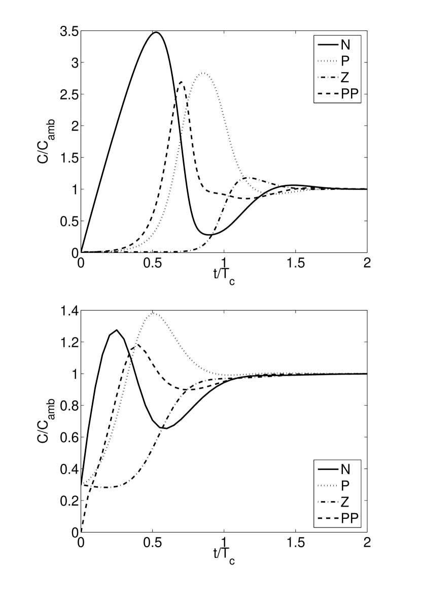
Figure 3: The time evolution of the concentrations ($C$) of the species and the primary productivity. Starting concentrations are $0.01\times$ steady state concentrations of $N$, $P$ and $Z$ (top) and $0.3\times$ steady state concentrations of $N$, $P$ and $Z$ (bottom).

3.2 The residence time of fluid parcels in the wake

As pointed out in Sandulescu et al. (2007b) the hydrodynamic mesoscale structures are important for the enhancement of primary production in the wake of the island. To gain more insight into the interplay of hydrodynamics and plankton growth we now quantify the time scales for the relevant hydrodynamic processes. To this end we study the various structures in the hydrodynamic flow which have a significant influence on the residence times of nutrients and plankton in the wake of the island. Firstly, far away from the island (top and bottom of Fig. 1) the flow is strain dominated and particles like nutrients and plankton are advected with the background flow of speed $u_{0}$. Thus the residence time of particles released away from the island (with $y>2$ and $y<-2$, $x=0$) is about 16 days.

Figure 4: The trajectory of a fluid parcel released in the flow at the coordinates (-1.15, 0) at time $t=0$. Its subsequent positions are plotted with a dimensionless time step $\Delta t=0.001$.

Secondly we note the existence of the eddies. They are characterized by a dominance of vorticity compared to strain. Thus particles are trapped in the vortex once entrained to it. The particles will rotate in the vortex for some time, but since this confinement is not perfect and vortices exist only for some time they leave the vortex and move away with the background flow out of the computational area (cf. Fig. 4).

Figure 5: The unstable manifold of the chaotic saddle. Snapshots taken at $t=1.5\ T_{c}$ (lower plot), and $2\ T_{c}$ (upper plot).

Thirdly we consider two other geometrical objects which are also relevant for the residence time of particles in the vortex street: the chaotic saddle and the cylinder boundary. As shown in (Jung et al., 1993; Duan and Wiggins, 1997) there exists a chaotic saddle which is embedded in the flow beyond the island. At least for short time scales, this invariant set determines the residence times of particles. Particles released in the neighborhood of the chaotic saddle will approach it along its stable manifold and will leave it along its unstable manifold. The unstable manifolds at two different times (the manifolds and the saddle are time-dependent) are presented in Fig. 5. As compared with the configuration in Jung et al. (1993), the manifolds are tightly packed close to the cylinder, because of the parameters used here. To obtain an estimate for the residence time on the chaotic saddle we use a method suggested by Jung et al. (1993). We sprinkle a large number $N$ of tracer particles ($N=62500$) in the area $[0,2]\times[-1,1]$ and integrate their trajectories forward in time. If the dynamics in the region is mainly hyperbolic, the number of particles remaining in the area of the chaotic saddle decreases as $N~{}\sim~{}\exp(-\kappa~{}t)$ with $\kappa$ the escape rate or $1/\kappa$ the mean residence time on the saddle. Figure 6 shows the residence times obtained with this method, and Fig. 7 shows the decay of the number of particles in the region as a function time. We note that the expected exponential decay occurs only for very short time scales. By fitting this initial time decay, the corresponding escape rate is $\kappa=3.1/T_{c}$, and therefore the residence time of tracers in the hyperbolic part of the saddle is $\tau~{}\sim~{}10$ days. For larger times the particle number in the region decays as a power law. The reason for this power-law behavior is the non-hyperbolic dynamics near the boundary of the cylinder. As already shown by (Jung et al., 1993) particles stay for a long time in the vicinity of the cylinder giving rise to another long-term statistics of the residence times of the tracers. Thus the number of particles decays as $N\sim t^{-\gamma}$ with $\gamma=0.96$. The residence times in the vicinity of the island can be estimated as $\tau~{}\sim~{}85$ days, measured from the decay to a fraction $e$ of the initial number: $N(\tau)=N(0)/e$.

Overall we obtain a residence time statistics which reflects a combination of the three components in the flow: the cylinder, the chaotic saddle and the vortices. This leads to residence times of tracers in the wake as long as $90$ days (cf. Fig. 6). Note that in Fig. 6 one can see that tracers having the longer residence times are either located close to the cylinder or on the chaotic saddle. The residence times in the vortices are determined by their travel time which is about 50 days.

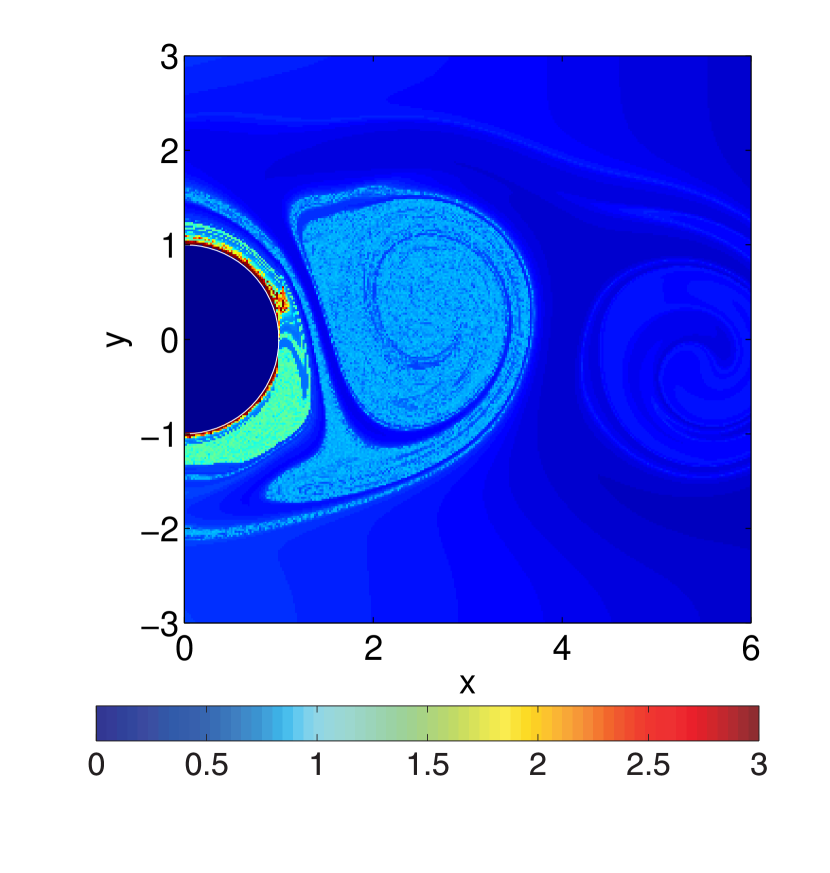
Figure 6: Residence time (coded in color in units of $T_{c}$) of fluid elements inside the area as a function of its initial positions at time $t/T_{c}=0.25$.

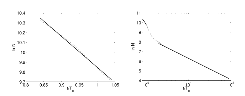
Figure 7: The number $N$ of tracers inside the area $[0,2]\times[-1,1]$ as a function of time in units of the period of the flow $T_{c}$. Vortex strength $w=200$. Left panel shows the very early decay, with an exponential fit. Right panel plots the overall decay, with a power law fit at large times.

3.3 The interplay of biological and hydrodynamical residence times

To understand the emergence of localized enhancement of primary production we have to analyze the interplay of the different time scales relevant for coupled biological and hydrodynamical processes. Biological evolution needs about 30-60 days to reach the steady-state when entering the computational domain with very low concentrations of nutrients and plankton. Due to the exponential growth in the beginning of the growth phase, we obtain a plankton bloom after about 25 days. Outside the vortex street the travel time of tracers through the computational domain is only about 16 days due to the background flow of $u_{0}=0.18$ m/s. Therefore we cannot expect a considerable growth of plankton outside the vortex street, since the residence time of plankton and nutrients is too short.

Let us now analyze the situation within the mesoscale structures of the flow in the wake of the island. As the residence time close to the island is about 85 days the concentrations of nutrients and plankton have already reached the steady-state which is also indicated by the green color in the right column of Fig. 2. Some of the particles in the vicinity of the island come close to the stable manifold of the chaotic saddle visible as the filaments which detach from the cylinder. These filaments are stretched and folded along the unstable manifold of the chaotic saddle, being diffusively diluted during the process by mixing with the poor surrounding waters. Thus, very thin filaments of low plankton and nutrient concentration are produced which are first rolled around the vortices and then entrained by them. Inside the vortex the concentrations become homogeneised to a low value. These very low concentrations of plankton experience the bloom cycle described in Section 3.1 during the time they are trapped and confined by the vortex. Since the travel time for the vortices is about 50 days, plankton in them has time to grow. Therefore we observe a localized plankton bloom when the vortex has travelled a distance of $\sim 100$ km which corresponds to a residence of the plankton in the vortices of $\sim 15-20$ days. After 40-50 days and $\sim 200$ km we obtain steady-state concentrations and the former filamental structure within the vortex is smeared out by our diffusion term which mimics small scale turbulence.

3.4 The emergence of filamental structures due to strong mixing

In the previous subsection we have stated that the transport of nutrients and plankton from the vicinity into the interior of a vortex happens by filaments which are entrained by the vortex. To explain this stretching mechanism we now study the mixing process around the vortices in more detail using a method to visualize exponential divergence of the trajectories of initially nearby particles.

The usual tool to analyse exponential divergence in dynamical systems theory is the computation of Lyapunov exponents. In order to adjust this concept to local processes, we compute finite size Lyapunov exponents (FSLE) which are based on the idea that one measures the time necessary to obtain a final prescribed distance $\delta_{f}$ starting from an initial distance $\delta_{0}$ (Artale et al., 1997; d’Ovidio et al., 2004). For a two-dimensional flow we obtain two Lyapunov exponents $\lambda_{+}$ and $\lambda_{-}$ (see appendix B).

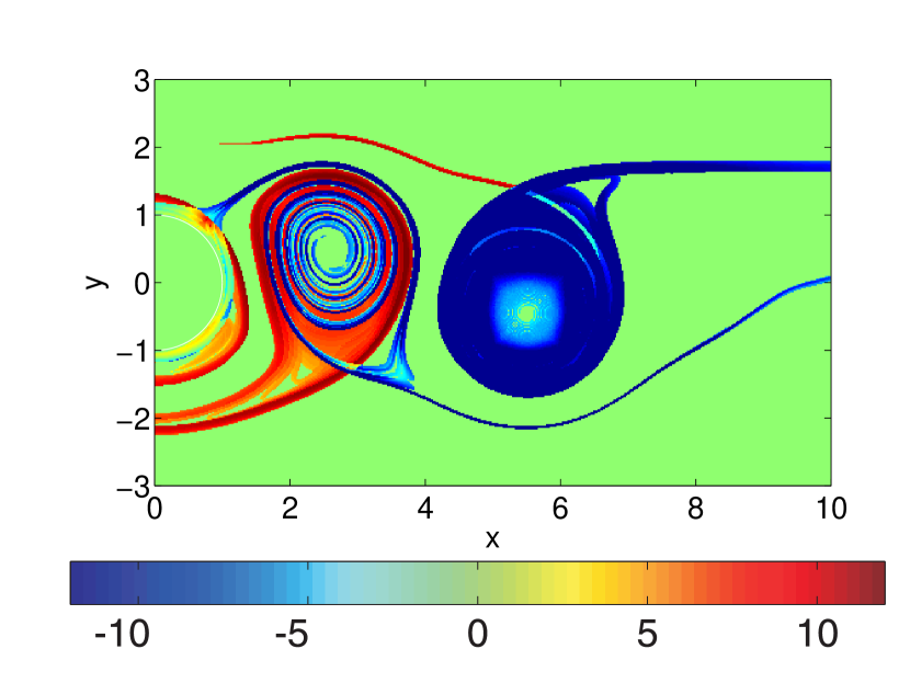
Figure 8: Finite Size Lyapunov Exponent distributions. We plot the field $\lambda_{+}-|\lambda_{-}|$ at time $t/T_{c}=0.25$. Stable and unstable manifolds in the flow are approximated by the most positive and most negative filaments in the distributions.

Maxima in the spatial distribution of $\lambda_{+}$, the positive or expanding FSLE, approximate the underlying stable manifold of the chaotic flow (Joseph and Legras, 2002; d’Ovidio et al., 2004), the direction along which parcels approach the saddle. The contracting FSLE, $\lambda_{-}$, detects the underlying unstable manifold of the chaotic flow, the direction along which parcels are stretched out of the saddle. For details on how to calculate these scalar fields see Appendix B.

The FSLEs were calculated choosing the initial separation $\delta_{0}$ equal to the gridsize and the final separation $\delta_{f}$ equal to the radius of the island and the vortices, since this is the scale of the motion in the wake. As both stable and unstable manifolds cannot be crossed by fluid parcels they are barriers (Artale et al., 1997; d’Ovidio et al., 2004). The scalar field $\lambda_{+}-|\lambda_{-}|$ is plotted in Fig. 8. FSLEs are Lagrangian measures, which are computed from trajectories that remain in the flow for a long time, in our case for up to $3T_{c}$. Therefore even though they are plotted as a snapshot, the visualized structures reflect the stretching and folding of the fluid parcels during this long time. The stable and unstable manifolds are intertwined around the vortex cores and at the island. Stable and unstable manifolds are crossing the wake allowing for transport across the vortex street. They intersect each other in hyperbolic points, regions of strong mixing. This stretching-compressing mechanism leads to low nutrient and plankton concentrations transported into the interior of the vortex, and thus becoming the starting concentrations for the localized plankton bloom.

3.5 On the role of the upwelling region of nutrients

Finally we discuss the importance of the vertical mixing of nutrients in the upwelling zone for the emergence of a plankton bloom inside vortices. Comparing Fig. 2 left and right column it is obvious that in the case of an inflow with steady-state conditions (left column), the nutrient plume which appears in the neighborhood of the upwelling zone gives rise to a phytoplankton bloom (red filamental plume). Such a plume is almost absent under low inflow conditions (right column). Though the nutrient supply due to vertical mixing is identical for both inflow conditions, it seems to have a limited effect in the low inflow case. One argument has been already discussed above: The background flow transports the nutrients too fast so that the very small plankton concentrations can not grow to reach high values during the travel time through the computational area. The growth of phytoplankton is visible only further downstream. This leads to the conclusion that the plankton bloom inside the vortex is only slightly influenced by the extra nutrients entrained from the upwelling zone in the low inflow situation. To strengthen this statement we present in Fig. 9 the plankton dynamics when the upwelling is removed. We note that the concentration values for phytoplankton and zooplankton are slightly lower compared to the upwelling regime, but qualitatively there is no change observable. Thus localized phytoplankton blooms in vortices are possible in the wake of an island just due to the mechanism discussed in Subsec. 3.4 without any extra nutrient supply due to upwelling.

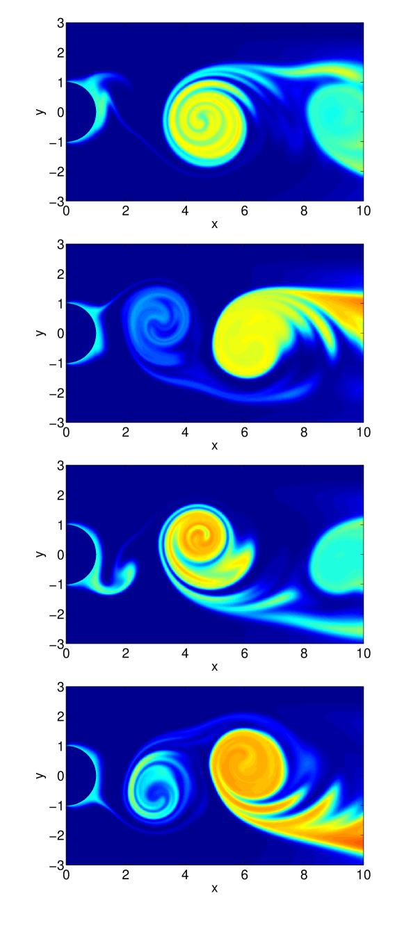
Figure 9: The concentration of phytoplankton in the absence of upwelling. Snapshots taken at $t/T_{c}=4.1,4.35,4.6,4.85$. The color coding is in the same range as in Fig. 2.

4 Conclusions

We have analyzed the interplay between hydrodynamic mesoscale structures and biological growth in the wake of an island. Parameter values for the kinematic hydrodynamic flow were chosen to match the observations for the Canary island region, but since the basic hydrodynamic features studied here are commonly observed in other areas too, we expect our results to be of general validity. Our study is focused on the emergence of a plankton bloom localized in a vortex in the wake of an island. In a previous paper (Sandulescu et al., 2007b) it has been pointed out that under certain conditions a vortex may act as an incubator for plankton growth and primary production. Here we have revealed the mechanism of such a plankton bloom. If the hydrodynamic flow far away from the island is dominated by a jet, then the hydrodynamic time scale is much faster than the biological one, so that considerable growth of plankton cannot be observed. By contrast, in the wake of an island we obtain a much slower time scale which becomes comparable to the biological one giving rise to an exponential growth of phytoplankton and thus to the emergence of a plankton bloom within a vortex. The essential factors for this phenomenon to happen are (i) the long residence times in the vicinity of the island leading to an enrichment of nutrients and plankton in the neighborhood of the island; (ii) the transport and subsequent entrainment of nutrients and plankton to the interior of the vortex due to filamental structures emerging with the chaotic saddle beyond the island, and (iii) the confinement of plankton in the vortex. Though the upwelling of nutrients in an upwelling zone enhances the emergence of localized plankton blooms, it is not a precondition for this phenomenon to occur. The extra nutrients supplied by vertical mixing in areas away from the vortex street are not a part of the mechanism explained here. Upwelling could be more effective if the vortices directly cross upwelling zones when travelling through the ocean. Similar situations have been considered in (Martin et al., 2002; Pasquero et al., 2005). There it has been shown that under conditions where upwelling occurs only directly within vortices, a plankton bloom within a vortex can be initiated. Therefore this mechanism, which relies mostly on upwelling, is different from the one reported here. The variety of real observations (Arístegui et al., 1997) in the Canary wake may benefit from the identification of the different possible mechanisms.

Appendix A: The numerical algorithm

The investigation of the interplay of biological and physical processes is based on advection-reaction-diffusion systems (Eqs. 6). This system of partial differential equations is solved numerically by means of a semi-Lagrangian algorithm. The concentration fields of nutrients $N$, phytoplankton $P$ and zooplankton $Z$ are represented on a grid of [500 x 300] points. The integration scheme splits the computation into three steps corresponding to advection, reaction and diffusion which are performed sequentially in the following way:

1. Advection: Each point of the grid is integrated for a time step $dt$ backwards in time along the trajectory of a fluid parcel in the velocity field. This procedure yields the position from which a fluid parcel would have reached the chosen grid point. Typically this position is not located on a grid point but somewhere in between.

2. Reaction: Once the position of the fluid parcel in the past is found, we compute the values of the concentration fields of $N$, $P$ and $Z$ at this point and take them as initial values for the reaction term which is integrated forward in time for a time step $dt$. Since the position of the fluid parcel is not on a grid point the concentration fields have to be evaluated by means of a bilinear interpolation using the nearest neighbor grid points.

3. Diffusion: Finally we perform a diffusion step based on an Eulerian scheme. Note, that the reaction step induces already a numerical diffusion of the order $D_{n}\propto dx^{2}/dt$ due to the interpolation. Therefore one has to make sure that the real diffusion according to the Okubo estimate ( $D=10m^{2}/s$, dimensionless value $D=0.041472$) (Okubo, 1971) is larger than this numerical diffusion. Additionally the stability condition of the Eulerian diffusion step ($Ddt_{d}/dx^{2}<1$ with $dt_{d}$ the diffusion time step) has to be fulfilled. Both conditions together require that the diffusion time step $dt_{d}$ is much smaller than $dt$. We have chosen $dt_{d}=dt/10$ in our algorithm, i.e. after each step of advection and reaction we perform 10 steps of diffusion. The parameters used in the computation are $dx=0.02$, $dt=0.01$ and $dt_{d}=0.001$ expressed in units of $T_{c}=30~{}days$ for time and $r=25~{}km$ for space.

Appendix B: Finite Size Lyapunov-Exponents

Stretching by advection in fluid flows is often described by means of Lyapunov exponents. They are defined as the average of the exponential rate of separation of initially infinitesimally separated parcels. For application with data sets from tracer experiments the infinite time limit poses a problem. To study non-asymptotic dispersion processes, Finite Size Lyapunov Exponents (FSLE) have been introduced (Artale et al., 1997; d’Ovidio et al., 2004). The FSLE technique allows us to characterize dispersion processes and to detect and visualize Lagrangian structures, such as barriers and vortices. The FSLE are computed by starting two fluid elements at time $t$ close to the point ${\bf x}$ but at a small distance $\delta_{0}$, and let them to evolve until their separation exceeds $\delta_{f}$. From the elapsed time, $\tau_{+}$, the FSLE is calculated as

$$\lambda_{+}({\bf x},t,\delta_{0},\delta_{f})=\frac{1}{\tau_{+}}\log\frac{\delta_{f}}{\delta_{0}}$$ (7)

The positive subindexes indicate that the tracers are advected forward in time. $\lambda_{+}$ is a scalar measure giving the stretching rate in the flow as it is the inverse of the separation time $\tau$.

The same definition can be applied to tracers integrated in the negative direction in time. $\lambda_{-}$ gives the contraction rate in the flow at the specified position:

$$\lambda_{-}({\bf x},t,\delta_{0},\delta_{f})=\frac{1}{\tau_{-}}\log\frac{\delta_{f}}{\delta_{0}}$$ (8)

Regions with high values of $\lambda_{+}$ and $\lambda_{-}$ trace out approximately the stable and unstable manifolds of the chaotic saddle. These manifolds cannot be crossed by fluid parcel trajectories and thus greatly influence the transport in the area.

References

- Abraham (1998) Abraham, E.: The generation of plankton patchiness by turbulent stirring, Nature, 391, 577–580, 1998.
- Arístegui et al. (1997) Arístegui, J., Tett, P., Hernández-Guerra, A., Basterretxea, G., Montero, M. F., Wild, K., Sangrá, P., Hernández-Leon, S., Canton, M., García-Braun, J. A., Pacheco, M., and Barton, E.: The influence of island-generated eddies on chlorophyll distribution: a study of mesoscale variation around Gran Canaria, Deep Sea Research I, 44, 71–96, 1997.
- Arístegui et al. (2004) Arístegui, J., Barton, E. D., Tett, P., Montero, M. F., García-Muñoz, M., Basterretxea, G., Cussatlegras, A.-S., Ojeda, A., and de Armas, D.: Variability in plankton community structure, metabolism, and vertical carbon fluxes along an upwelling filament (Cape Juby, NW Africa), Progress in Oceanography, 62, 95–113, 2004.
- Artale et al. (1997) Artale, V., Boffetta, G., Celani, M., Cencini, M., and Vulpiani, A.: Dispersion of passive tracers in closed basins: Beyond the diffusion coefficient, Phsy. Fluids, 9, 3162–3171, 1997.
- Baretta et al. (1997) Baretta, J., Baretta, J., and Ebenhöh, W.: Microbial dynamics in the marine ecosystems model ERSEM II with decoupling carbon assimilation and nutrient uptake, JSR, 38, 195 – 212, 1997.
- Bracco et al. (2000) Bracco, A., Provenzale, A., and Scheuring, I.: Mesoscale vortices and the paradox of the plankton, Proc. Roy. Soc. Lond. B, 267, 1795–1800, 2000.
- Denman and Gargett (1995) Denman, K. and Gargett, A.: Biological-physical interactions in the upper ocean: the role of vertical and small scale transport processes, Annu. Rev. Fluid Mech., 27, 225–255, 1995.
- d’Ovidio et al. (2004) d’Ovidio, F., Fernández, V., Hernández-García, E., and López, C.: Mixing structures in the Mediterranean Sea from finite-size Lyapunov exponents, Geophysical Research Letters, 31, L17 203, 2004.
- Duan and Wiggins (1997) Duan, J. and Wiggins, S.: Lagrangian transport and chaos in the near wake of the flow around an obstacle: a numerical implementation of lobe dynamics, Nonlin. Proc. Geophys., 4, 125–136, 1997.
- Edwards and Bees (2001) Edwards, M. and Bees, M.: Generic dynamics of a simple plankton population model with a non-integer exponent of closure, Chaos, Solitons & Fractals, 12, 289, 2001.
- Edwards and Brindley (1996) Edwards, M. and Brindley, J.: Oscillatory behavior in a three-component plankton population model, Dyn. Stab. Sys., 11, 347–370, 1996.
- Hernández-García and López (2004) Hernández-García, E. and López, C.: Sustained plankton blooms under open chaotic flows, Ecol. Complex., 1, 253–259, 2004.
- Hernández-García et al. (2002) Hernández-García, E., López, C., and Neufeld, Z.: Small-scale structure of nonlinearly interacting species advected by chaotic flows, Chaos, 12, 470–480, 2002.
- Hernández-García et al. (2003) Hernández-García, E., López, C., and Neufeld, Z.: Spatial Patterns in Chemically and Biologically Reacting Flows, in: Chaos in Geophysical Flows, edited by Bofetta, G., Lacorata, G., Visconti, G., and Vulpiani, A., OTTO Editore, Torino, 2003.
- Huppert et al. (2002) Huppert, A., Blasius, B., and Stone, L.: A model of phytoplankton blooms, American Naturalist, 159, 156–171, 2002.
- Joseph and Legras (2002) Joseph, B. and Legras, B.: Relation between kinematic boundaries, stirring, and barriers for the Antartic Polar vortex, J. Atm. Sci., 59, 1198–1212, 2002.
- Jung et al. (1993) Jung, C., Tél, T., and Ziemniak, E.: Application of scattering chaos to particle transport in a hydrodynamical flow, Chaos, 3, 555–568, 1993.
- Károlyi et al. (2000) Károlyi, G., Péntek, A., Scheuring, I., Tél, T., and Toroczkai, Z.: Chaotic flow: the physics of species coexistence, Proc. Natl. Acad. Sci. USA, 97, 13 661–13 665, 2000.
- López et al. (2001a) López, C., Hernández-García, E., Piro, O., Vulpiani, A., and Zambianchi, E.: Population dynamics advected by chaotic flows: A discrete-time map approach, Chaos, 11, 397–403, 2001a.
- López et al. (2001b) López, C., Neufeld, Z., Hernández-García, E., and Haynes, P.: Chaotic advection of reacting substances: Plankton dynamics on a meandering jet, Phys. Chem. Earth, B 26, 313–317, 2001b.
- Mann and Lazier (1991) Mann, K. and Lazier, J.: Dynamics of marine ecosystems. Biological-physical interactions in the oceans, Blackwell Scientific Publications, Boston, 1991.
- Martin (2003) Martin, A.: Phytoplankton patchiness: the role of lateral stirring and mixing, Progress in Oceanography, 57, 125–174, 2003.
- Martin et al. (2002) Martin, A., Richards, K., Bracco, A., and Provenzale, A.: Patchy productivity in the open ocean, Global Biogeochemical Cycles, 16, 10.1029/2001GB001 449, 2002.
- Okubo (1971) Okubo, A.: Oceanic diffusion diagrams, Deep-Sea Res., 18, 789, 1971.
- Oschlies and Garçon (1999) Oschlies, A. and Garçon, V.: An eddy-permitting coupled physical-biological model of the North-Atlantic, sensitivity to advection numerics and mixed layer physics, Global Biocheochem. Cycles, 13, 135–160, 1999.
- Pasquero et al. (2004) Pasquero, C., Bracco, A., and Provenzale, A.: Coherent vortices, Lagrangian particles and the marine ecosystem, in: Shallow Flows, edited by Uijttewaal, W. and Jirka, G., pp. 399–412, Balkema Publishers, Leiden, 2004.
- Pasquero et al. (2005) Pasquero, C., Bracco, A., and Provenzale, A.: Impact of spatiotemporal viariability of the nutrient flux on primary productivity in the ocean, J. Geophys. Res. 11, 1–13, 2005.
- Peters and Marrasé (2000) Peters, F. and Marrasé, C.: Effects of turbulence on plankton: an overview of experimental evidence and some theoretical considerations, Mar. Ecol. Prog. Ser., 205, 291–306, 2000.
- Sandulescu et al. (2006a) Sandulescu, M., Hernández-García, E., López, C., and Feudel, U.: Kinematic studies of transport across an island wake, with application to the Canary islands, Tellus A, 58, 605–615, 2006a.
- Sandulescu et al. (2007b) Sandulescu, M., Hernández-García, E., López, C., and Feudel, U.: Biological activity in the wake of an island close to a costal upwelling, submitted to Ecological Complexity, 2007b.
- Steele and Henderson (1981) Steele, J. and Henderson, E.: A simple plankton model, The American Naturalist, 117, 676–691, 1981.
- Steele and Henderson (1992) Steele, J. and Henderson, E.: The role of predation in plankton models, J. Plankton Res., 14, 157–172, 1992.