Polynomial Filtering for Fast Convergence in Distributed Consensus

Abstract

In the past few years, the problem of distributed consensus has received a lot of attention, particularly in the framework of ad hoc sensor networks. Most methods proposed in the literature address the consensus averaging problem by distributed linear iterative algorithms, with asymptotic convergence of the consensus solution. The convergence rate of such distributed algorithms typically depends on the network topology and the weights given to the edges between neighboring sensors, as described by the network matrix. In this paper, we propose to accelerate the convergence rate for given network matrices by the use of polynomial filtering algorithms. The main idea of the proposed methodology is to apply a polynomial filter on the network matrix that will shape its spectrum in order to increase the convergence rate. Such an algorithm is equivalent to periodic updates in each of the sensors by aggregating a few of its previous estimates. We formulate the computation of the coefficients of the optimal polynomial as a semi-definite program that can be efficiently and globally solved for both static and dynamic network topologies. We finally provide simulation results that demonstrate the effectiveness of the proposed solutions in accelerating the convergence of distributed consensus averaging problems.

1 Introduction

We consider the problem of distributed consensus [1] that has become recently very interesting especially in the context of ad hoc sensor networks. In particular, the problem of distributed average consensus has attracted a lot of research efforts due to its numerous applications in diverse areas. A few examples include distributed estimation [2], distributed compression [3], coordination of networks of autonomous agents [4] and computation of averages and least-squares in a distributed fashion (see e.g., [5, 6, 7, 8] and references therein).

In general the main goal of distributed consensus is to reach a global solution using only local computation and communication while staying robust to changes in the network topology. Given the initial values at the sensors, the problem of distributed averaging is to compute their average at each sensor using distributed linear iterations. Each distributed iteration involves local communication among the sensors. In particular, each sensor updates its own local estimate of the average by a weighted linear combination of the corresponding estimates of its neighbors. The weights that are represented in a network weight matrix $W$ typically drive the importance of the measurements of the different neighbors.

One of the important characteristics of the distributed consensus algorithms is the rate of convergence to the asymptotic solution. In many cases, the average consensus solution can be reached by successive multiplications of $W$ with the vector of initial sensor values. Furthermore, it has been shown in [5] that in the case of fixed network topology, the convergence rate depends on the second largest eigenvalue of $W$, $\lambda_{2}(W)$. In particular, the convergence is faster when the value of $\lambda_{2}(W)$ is small. Similar convergence results have been proposed recently in the case of random network topology [9, 10], where the convergence rate is governed by the expected value of the $\lambda_{2}(W)$, $E[\lambda_{2}(W)]$.

The main research direction so far focuses on the computation of the optimal weights $W$ that yield the fastest convergence rate to the consensus solution [5, 6, 7]. In this work, we diverge from methods that are based on successive multiplications of $W$, and we rather allow the sensors to use their previous estimates, in order to accelerate the convergence rate. This is similar in spirit to the works proposed [12, 13] that reach the consensus solution in a finite number of steps. They use respectively extrapolation methods and linear dynamical system formulation for fixed network topologies. In order to address more generic network topologies, we propose here to use a matrix polynomial $p$ applied on the weight matrix $W$ in order to shape its spectrum. Given the fact that the convergence rate is driven by $\lambda_{2}(W)$, it is therefore possible to impact on the convergence rate by careful design of the polynomial $p$. In the implementation viewpoint, working with $p(W)$ is equivalent to each sensor aggregating its value periodically using its own previous estimates. We further formulate the problem of the computation of the optimal coefficients for both static and dynamic network topologies. We show that this problem can be efficiently and globally solved in both cases by the definition of a semi-definite program (SDP).

The rest of this paper is organized as follows. In Section 2 we review the main convergence results of average consensus in both fixed and dynamic random network topologies. Next, in Section 3 we introduce the polynomial filtering methodology and discuss its implementation for distributed consensus problems. We compute the optimal polynomial filter in Section 4 for both static and dynamic network topologies. In Section 5 we provide simulation results that verify the validity and the effectiveness of our method. Related work is finally presented in Section 6.

2 Convergence in Distributed Consensus Averaging

Let us first define formally the problem of distributed consensus averaging. Assume that initially each sensor $i$ reports a scalar value $x_{0}(i)\in\mathbb{R}$. We denote by $x_{0}=[x_{0}(1),\ldots,x_{0}(n)]^{\top}\in\mathbb{R}^{n}$ the vector of initial values on the network. Denote by

$$\mu=\frac{1}{n}\sum_{i=1}^{n}x_{0}(i)$$ (1)

the average of the initial values of the sensors. However, one rarely has a complete view of the network. The problem of distributed averaging therefore becomes typically to compute $\mu$ at each sensor by distributed linear iterations. In what follows we review the main convergence results for distributed consensus algorithms on both fixed and random network topologies.

2.1 Static network topology

We model the static network topology as an undirected graph $\mathcal{G}=(\mathcal{V},\mathcal{E})$ with nodes $\mathcal{V}=\{1,\ldots,n\}$ corresponding to sensors. An edge $(i,j)\in\mathcal{E}$ is drawn if and only if sensor $i$ can communicate with sensor $j$. We denote the set of neighbors for node $i$ as $\mathcal{N}_{i}=\{j|~{}(i,j)\in\mathcal{E}\}$. Unless otherwise stated, we assume that each graph is simple i.e., no loops or multiple edges are allowed.

In this work, we consider distributed linear iterations of the following form

$$x_{t+1}(i)=W_{ii}x_{t}(i)+\sum_{j\in\mathcal{N}_{i}}W_{ij}x_{t}(j),$$ (2)

for $i=1,\ldots,n$, where $x_{t}(j)$ represents the value computed by sensor $j$ at iteration $t$. Since the sensors communicate in each iteration $t$, we assume that they are synchronized. The parameters $W_{ij}$ denote the edge weights of $\mathcal{G}$. Since each sensor communicates only with its direct neighbors, $W_{ij}=0$ when $(i,j)\notin\mathcal{E}$. The above iteration can be compactly written in the following form

$$x_{t+1}=Wx_{t},$$ (3)

or more generally

$$x_{t}=\Big{(}\prod_{i=0}^{t-1}W\Big{)}x_{0}=W^{t}x_{0}.$$ (4)

We call the matrix $W$ that gathers the edge weights $W_{ij}$, as the weight matrix. Note that $W$ is a sparse matrix whose sparsity pattern is driven by the network topology. We assume that $W$ is symmetric, and we denote its eigenvalue decomposition as $W=Q\Lambda Q^{\top}$. The (real) eigenvalues can further be arranged as follows:

$$\lambda_{1}(W)\geq\lambda_{2}(W)\geq\ldots\geq\lambda_{n-1}(W)\geq\lambda_{n}(W).$$ (5)

The distributed linear iteration given in eq. (3) converges to the average if and only if

$$\lim_{t\rightarrow\infty}W^{t}=\frac{\textbf{1}\textbf{1}^{\top}}{n},$$ (6)

where 1 is the vector of ones [5]. Indeed, notice that in this case

$$x^{\ast}=\lim_{t\rightarrow\infty}x_{t}=\lim_{t\rightarrow\infty}W^{t}x_{0}=\frac{\textbf{1}\textbf{1}^{\top}}{n}x_{0}=\mu\textbf{1}.$$

It has been shown that for fixed network topology the convergence rate of eq. (3) depends on the magnitude of the second largest eigenvalue $\lambda_{2}(W)$ [5]. The asymptotic convergence factor is defined as

$$r_{\textrm{asym}}(W)=\sup_{x_{0}\neq\mu\textbf{1}}\lim_{t\rightarrow\infty}\Big{(}\frac{\|x_{t}-\mu\textbf{1}\|_{2}}{\|x_{0}-\mu\textbf{1}\|_{2}}\Big{)}^{1/t},$$ (7)

and the per-step convergence factor is written as

$$r_{\textrm{step}}(W)=\sup_{x_{0}\neq\mu\textbf{1}}\frac{\|x_{t+1}-\mu\textbf{1}\|_{2}}{\|x_{t}-\mu\textbf{1}\|_{2}}.$$ (8)

Furthermore, it has been shown that the convergence rate relates to the spectrum of $W$, as given by the following theorem [5].

Theorem 1

The convergence given by eq. (6) is guaranteed if and only if

$$\textbf{1}^{\top}W = \textbf{1}^{\top},$$ (9)

$$W\textbf{1} = \textbf{1},$$ (10)

$$\rho\big{(}W-\frac{\textbf{1}\textbf{1}^{\top}}{n}\big{)} < 1,$$ (11)

where $\rho(\cdot)$ denotes the spectral radius of a matrix. Furthermore,

$$r_{\textrm{asym}}(W)=\rho\big{(}W-\frac{\textbf{1}\textbf{1}^{\top}}{n}\big{)},$$ (12)

$$r_{\textrm{step}}(W)=\|W-\frac{\textbf{1}\textbf{1}^{\top}}{n}\|_{2}.$$ (13)

According to the above theorem, $\frac{1}{\sqrt{n}}\textbf{1}$ is a left and right eigenvector of $W$ associated with the eigenvalue one, and the magnitude of all other eigenvalues is strictly less than one. Note finally, that since $W$ is symmetric, the asymptotic convergence factor coincides with the per-step convergence factor, which implies that the relations (12) and (13) are equivalent.

We give now an alternate proof of the above theorem that illustrates the importance of the second largest eigenvalue in the convergence rate. We expand the initial state vector $x_{0}$ to the orthogonal eigenbasis $Q$ of $W$; that is,

$$x_{0}=\nu_{1}\frac{\textbf{1}}{\sqrt{n}}+\sum_{j=2}^{n}\nu_{j}q_{j},$$

where $\nu_{1}=\langle\frac{\textbf{1}}{\sqrt{n}},x_{0}\rangle$ and $\nu_{j}=\langle q_{j},x_{0}\rangle$. We further assume that $\nu_{1}\neq 0$. Then, eq. (4) implies that

$$x_{t} = W^{t}x_{0}=W^{t}\big{(}\frac{\nu_{1}}{\sqrt{n}}\textbf{1}+\sum_{j=2}^{n}\nu_{j}q_{j}\big{)}$$

$$= \frac{\nu_{1}}{\sqrt{n}}\textbf{1}+\sum_{j=2}^{n}\nu_{j}W^{t}q_{j}$$

$$= \frac{\nu_{1}}{\sqrt{n}}\textbf{1}+\sum_{j=2}^{n}\nu_{j}\lambda_{j}^{t}q_{j}.$$

Observe now that if $|\lambda_{j}|<1,~{}\forall j\geq 2$, then in the limit, the second term in the above equation decays and

$$x^{\ast}=\lim_{t\rightarrow\infty}x_{t}=\frac{\nu_{1}}{\sqrt{n}}\textbf{1}=\mu\textbf{1}.$$

We see that the smaller the value of $\lambda_{2}(W)$, the faster the convergence rate. Analogous convergence results hold in the case of dynamic network topologies discussed next.

2.2 Dynamic network topology

Let us consider now networks with random link failures, where the state of a link changes over the iterations. In particular, we use the random network model proposed in [9, 10]. We assume that the network at any arbitrary iteration $t$ is $\mathcal{G}(t)=(\mathcal{V},\mathcal{E}(t))$, where $\mathcal{E}(t)$ denotes the edge set at iteration $t$, or equivalently at time instant $t$. Since the network is dynamic, the edge set changes over the iterations, as links fail at random. We assume that $\mathcal{E}(t)\subseteq\mathcal{E}^{\ast}$, where $\mathcal{E}^{\ast}\subseteq\mathcal{V}\times\mathcal{V}$ is the set of realizable edges when there is no link failure.

We also assume that each link $(i,j)$ fails with a probability $(1-p_{ij})$, independently of the other links. Two random edge sets $\mathcal{E}(t_{1})$ and $\mathcal{E}(t_{2})$ at different iterations $t_{1}$ and $t_{2}$ are independent. The probability of forming a particular $\mathcal{E}(t)$ is thus given by $\prod_{(i,j)\in\mathcal{E}(t)}p_{ij}$. We define the matrix $P$ as

$$P_{ij}=\begin{cases}p_{ij}&\textrm{if}~{}(i,j)\in\mathcal{E}^{\ast}~{}\textrm{and}~{}i\neq j,\\ 0&\textrm{otherwise}.\end{cases}$$ (14)

The matrix $P$ is symmetric and its diagonal elements are zero, since it corresponds to a simple graph. It represents the probabilities of edge formation in the network, and the edge set $\mathcal{E}(t)$ is therefore a random subset of $\mathcal{E}^{\ast}$ driven by the $P$ matrix. Finally, the weight matrix $W$ becomes dependent on the edge set since only the weights of existing edges can take non zero values.

In the dynamic case, the distributed linear iteration of eq. (2) becomes

$$x_{t+1}(i)=W_{ii}(t)x_{t}(i)+\sum_{j\in\mathcal{N}_{i}}W_{ij}(t)x_{t}(j)$$ (15)

or in compact form,

$$x_{t+1}=W_{t}x_{t},$$ (16)

where $W_{t}$ denotes the weight matrix corresponding to the graph realization $\mathcal{G}(t)$ of iteration $t$. The iterative relation given by eq. (16) can be written as

$$x_{t}=\Big{(}\prod_{i=0}^{t-1}W_{i}\Big{)}x_{0}.$$

Clearly, $x_{t}$ now represents a stochastic process since the edges are drawn randomly. The convergence rate to the consensus solution therefore depends on the behavior of the product $\prod_{i=0}^{t-1}W_{i}$. We say that the algorithm converges if

$$\forall x_{0}\in\mathbb{R}^{n},~{}\lim_{t\rightarrow\infty}E\|x_{t}-\mu\textbf{1}\|=0.$$ (17)

We review now some convergence results from [10], which first shows that

Lemma 1

For any $x_{0}\in\mathbb{R}^{n}$,

$$\|x_{t+1}-\mu\textbf{1}\|\leq\Big{(}\prod_{i=0}^{t}\rho\big{(}W_{i}-\frac{\textbf{1}\textbf{1}^{\top}}{n}\big{)}\Big{)}\|x_{0}-\mu\textbf{1}\|.$$

It leads to the following convergence theorem [10] for dynamic networks.

Theorem 2

If $E[\rho\big{(}W-\frac{\textbf{1}\textbf{1}^{\top}}{n}\big{)}\Big{)}]<1$, the vector sequence $\{x_{t}\}_{t=0}^{\infty}$ converges in the sense of eq. (17).

We define the convergence factor in dynamic network topologies as

$$r_{d}(W)=E\Big{[}\rho\big{(}W-\frac{\textbf{1}\textbf{1}^{\top}}{n}\big{)}\Big{]}.$$

This factor depends in general on the spectral properties of the induced network matrix and drives the convergence rate of eq. (16). The authors in [14] show that $|\lambda_{2}(E[W])|<1$ is also a necessary and sufficient condition for asymptotic (almost sure) convergence of the consensus algorithm in the case of random networks, where both network topology and weights are random (in particular i.i.d and independent over time).

Finally, it is interesting to note that the consensus problem in a random network relates to gossip algorithms. Distributed averaging under the synchronous gossip constraint implies that multiple node pairs may communicate simultaneously only if these node pairs are disjoint. In other words, the set of links implied by the active node pairs forms a matching of the graph. Therefore, the distributed averaging problem described above is closely related to the distributed synchronous algorithm under the gossip constraint that has been proposed in [15, Sec. 3.3.2]. It has been shown in this case that the averaging time (or convergence rate) of a gossip algorithm depends on the second largest eigenvalue of a doubly stochastic network matrix.

3 Accelerated consensus with polynomial filtering

3.1 Exploiting memory

As we have seen above, the convergence rate of the distributed consensus algorithms depends in general on the spectral properties of an induced network matrix. This is the case for both fixed and random network topologies. Most of the research work has been devoted to finding weight matrix $W$ for accelerating the convergence to the consensus solution when sensors only use their current estimates. We choose a different approach where we exploit the memory of sensors, or the values of previous estimates in order to augment to convergence rate.

Therefore, we have proposed in our previous work [12] the Scalar Epsilon Algorithm (SEA) for accelerating the convergence rate to the consensus solution. SEA belongs to the family of extrapolation methods for accelerating vector sequences, such as eq. (3). These methods exploit the fact that the fixed point of the sequence belongs to the subspace spanned by any $\ell+1$ consecutive terms of it, where $\ell$ is the degree of the minimal polynomial of the sequence generator matrix (for more details, see [12] and references therein). SEA is a low complexity algorithm, which is ideal for sensor networks and it is known to reach the consensus solution in $2\ell$ steps. However, $\ell$ is unknown in practice, so one may use all the available terms of the vector sequence. Hence, the memory requirements of SEA are $O(T)$, where $T$ is the number of terms. Moreover, SEA assumes that the sequence generator matrix (e.g., $W$ in the case of eq. (3)) is fixed, so that it does not adapt easily to dynamic network topologies.

In this paper, we propose a more flexible algorithm based on the polynomial filtering technique. Polynomial filtering permits to “shape” the spectrum of a certain symmetric weight matrix, in order to accelerate the convergence to the consensus solution. Similarly to SEA, it allows the sensors to use the value of their previous estimates. However, the polynomial filtering methodology introduced below presents three main advantages: (i) it is robust to dynamic topologies (ii) it has explicit control on the convergence rate and (iii) its memory requirements can be adjusted to the memory constraints imposed by the sensor.

3.2 Polynomial filtering

Starting from a given (possibly optimal) weight matrix $W$, we propose the application of a polynomial filter on the spectrum of $W$ in order to impact the magnitude of $\lambda_{2}(W)$ that mainly drives the convergence rate. Denote by $p_{k}(\lambda)$ the polynomial filter of degree $k$ that is applied on the spectrum of $W$,

$$p_{k}(\lambda)=\alpha_{0}+\alpha_{1}\lambda+\alpha_{2}\lambda^{2}+\ldots+\alpha_{k}\lambda^{k}.$$ (18)

Accordingly, the matrix polynomial is given as

$$p_{k}(W)=\alpha_{0}I+\alpha_{1}W+\alpha_{2}W^{2}+\ldots+\alpha_{k}W^{k}.$$ (19)

Observe now that

$$p_{k}(W) = p_{k}(Q\Lambda Q^{\top})$$ (20)

$$= \alpha_{0}I+\alpha_{1}(Q\Lambda Q^{\top})+\ldots+\alpha_{k}(Q\Lambda^{k}Q^{\top})$$

$$= Qp_{k}(\Lambda)Q^{\top},$$

which implies that the eigenvalues of $p_{k}(W)$ are simply the polynomial filtered eigenvalues of $W$ i.e., $p_{k}(\lambda_{i}(W)),~{}i=1,\ldots,n$.

In the implementation level, working on $p_{k}(W)$ implies a periodic update of the current sensor’s value with a linear combination of its previous values. To see why this is true, we observe that:

$$x_{t+k+1} = p_{k}(W)x_{t}$$ (21)

$$= \alpha_{0}x_{t}+\alpha_{1}Wx_{t}+\ldots+\alpha_{k}W^{k}x_{t}$$

$$= \alpha_{0}x_{t}+\alpha_{1}x_{t+1}+\ldots+\alpha_{k}x_{t+k}.$$

A careful design of $p_{k}$ may impact the convergence rate dramatically. Then, each sensor typically applies polynomial filtering for distributed consensus by following the main steps tabulated in Algorithm 1.

Algorithm 1 Polynomial Filtered Distributed Consensus

1:  Input: polynomial coefficients $\alpha_{0},\ldots,\alpha_{k+1}$, tolerance $\epsilon$.

2:  Output: average estimate $\bar{\mu}$.

3:  Initialization:

4:   $\bar{\mu}_{0}=x_{0}(i)$.

5:   Set the iteration index $t=1$.

6:  repeat

7:     if mod($t,k+1$) ==0 then

8:        $x_{t}(i)=\alpha_{0}x_{t-k-1}(i)+\alpha_{1}x_{t-k}(i)+\alpha_{2}x_{t-k+1}(i)+\ldots+\alpha_{k}x_{t-1}(i)$ {polynomial filtered update}

9:        $x_{t}(i)=W_{ii}x_{t}(i)+\sum_{j\in\mathcal{N}_{i}}W_{ij}x_{t}(j)$.

10:     else

11:        $x_{t}(i)=W_{ii}x_{t-1}(i)+\sum_{j\in\mathcal{N}_{i}}W_{ij}x_{t-1}(j)$.

12:     end if

13:     Increase the iteration index $t=t+1$.

14:     $\bar{\mu}_{t}=x_{t}(i)$.

15:  until $\bar{\mu}_{t}-\bar{\mu}_{t-1}<\epsilon$

Note that, for both fixed and random network topology cases, the $\alpha_{k}$’s are computed off-line assuming that $W$ and respectively $E[W]$ are known a priori. In what follows, we propose different approaches for computing the coefficients $\alpha_{i}$ of the filter $p_{k}$.

3.3 Newton’s interpolating polynomial

One simple and rather intuitive approach for the design of the polynomial $p_{k}(\lambda)$ is to use Hermite interpolation. Recall that the objective is to dampen the smallest eigenvalues $\lambda_{2},\ldots,\lambda_{n}$ of $W$, while keeping the eigenvalue one intact. Therefore, we assume that the spectrum of $W$ lies in an interval $[a,1]$ and we impose smoothness constraints of $p_{k}$ at the left endpoint $a$. In particular, the polynomial $p_{k}(\lambda):[a,1]\rightarrow\mathbb{R}$ that we seek, will be determined by the following constraints:

$$p_{k}(a) = 0,~{}p_{k}^{(i)}(a)=0,~{}i=1,\ldots,k-1$$ (22)

$$p_{k}(1) = 1,$$ (23)

where $p_{k}^{(i)}(a)$ denotes the $i$-th derivative of $p_{k}(\lambda)$ evaluated at $a$. The dampening is achieved by imposing smoothness constraints of the polynomial on the left endpoint of the interval. The computed polynomial will have degree equal to $k$. Finally, the coefficients of $p_{k}$ that satisfies the above constraints can be computed by the Newton’s divided differences table.

Figure 1 shows the form of $p_{k}(\lambda)$ for $a=0$ and different values of the degree $k$. As $k$ increases, the dampening of the small eigenvalues becomes more effective. It is worth mentioning that the design of Newton’s polynomial does not depend on the network size or the size of the weight matrix $W$. What is only needed is a left endpoint $a$, which encloses the spectrum of $W$, as well as the desired degree $k$, which moreover may be imposed by memory constraints. This feature of Newton’s polynomial is very interesting and it is particularly appealing in the case of dynamic network topologies. However, the above polynomial design is mostly driven by intuitive arguments, which tend to obtain small eigenvalues for faster convergence. In the following section, we provide an alternative technique for computing the polynomial filter that optimizes the convergence rate.

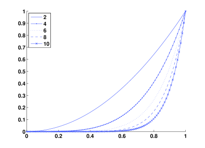
Figure 1: Newton’s polynomial of various degrees $k$.

4 Optimal polynomial filters

4.1 Polynomial filtering for static network topologies

We are now interested in finding the polynomial that leads to the fastest convergence of linear iteration described in eq. (3), for a given weight matrix $W$ and a certain degree $k$. For notational ease, we call $W_{p}=p_{k}(W)=\sum_{i=0}^{k}\alpha_{i}W^{i}$. According to Theorem 1, the optimal polynomial is the one that minimizes the second largest eigenvalue of $W_{p}$, i.e., $\rho\big{(}W_{p}-\frac{\textbf{1}\textbf{1}^{\top}}{n}\big{)}$. Therefore, we need to solve an optimization problem where the optimization variables are the $k+1$ polynomial coefficients $\alpha_{0},\ldots,\alpha_{k}$ and the objective function is the spectral radius of $W_{p}-\frac{\textbf{1}\textbf{1}^{\top}}{n}$.

Optimization problem: OPT1 $\min_{\alpha\in\mathbb{R}^{k+1}}~{}\rho\big{(}\sum_{i=0}^{k}\alpha_{i}W^{i}-\frac{\textbf{1}\textbf{1}^{\top}}{n}\big{)}$ subject to    $\big{(}\sum_{i=0}^{k}\alpha_{i}W^{i}\big{)}\textbf{1}=\textbf{1}$.

Interestingly, the optimization problem OPT1 is convex. First, its objective function is convex, as stated in Lemma 2.

Lemma 2

For a given symmetric weight matrix $W$ and degree $k$, $\rho\big{(}\sum_{i=0}^{k}\alpha_{i}W^{i}-\frac{\textbf{1}\textbf{1}^{\top}}{n}\big{)}$ is a convex function of the polynomial coefficients $\alpha_{i}$’s.

Proof: Let $\beta,\gamma\in\mathbb{R}^{k+1}$ and $0\leq\theta\leq 1$. Since $W$ is symmetric, $\sum_{i=0}^{k}\alpha_{i}W^{i}$ is also symmetric. Hence, the spectral radius is equal to the matrix 2-norm. Thus, we have

$$\rho\big{(}\sum_{i=0}^{k}(\theta\beta_{i}+(1-\theta)\gamma_{i})W^{i}-\frac{\textbf{1}\textbf{1}^{\top}}{n}\big{)}$$

$$= \Big{\|}\sum_{i=0}^{k}(\theta\beta_{i}+(1-\theta)\gamma_{i})W^{i}-\frac{\textbf{1}\textbf{1}^{\top}}{n}\Big{\|}_{2}$$

$$= \Big{\|}\theta\Big{(}\sum_{i=0}^{k}\beta_{i}W^{i}-\frac{\textbf{1}\textbf{1}^{\top}}{n}\Big{)}+(1-\theta)\Big{(}\sum_{i=0}^{k}\gamma_{i}W^{i}-\frac{\textbf{1}\textbf{1}^{\top}}{n}\Big{)}\Big{\|}_{2}$$

$$\leq \theta\Big{\|}\sum_{i=0}^{k}\beta_{i}W^{i}-\frac{\textbf{1}\textbf{1}^{\top}}{n}\Big{\|}_{2}+(1-\theta)\Big{\|}\sum_{i=0}^{k}\gamma_{i}W^{i}-\frac{\textbf{1}\textbf{1}^{\top}}{n}\Big{\|}_{2}$$

$$\leq \theta\rho\Big{(}\sum_{i=0}^{k}\beta_{i}W^{i}-\frac{\textbf{1}\textbf{1}^{\top}}{n}\Big{)}+(1-\theta)\rho\Big{(}\sum_{i=0}^{k}\gamma_{i}W^{i}-\frac{\textbf{1}\textbf{1}^{\top}}{n}\Big{)},$$

which proves the Lemma. In addition, the constraint of OPT1 is linear which implies that the set of feasible $\alpha_{i}$’s is convex. As OPT1 minimizes a convex function over a convex set, the optimization problem is indeed convex.

In order to solve OPT1, we use an auxiliary variable $s$ to bound the objective function, and then we express the spectral radius constraint as a linear matrix inequality (LMI). Thus, we need to solve the following optimization problem.

Optimization problem: OPT2 $\min_{s\in\mathbb{R},\alpha\in\mathbb{R}^{k+1}}~{}s$ subject to    $-sI\preceq\sum_{i=0}^{k}\alpha_{i}W^{i}-\frac{\textbf{1}\textbf{1}^{\top}}{n}\preceq sI$,    $\big{(}\sum_{i=0}^{k}\alpha_{i}W^{i}\big{)}\textbf{1}=\textbf{1}$.

Recall that since $W$ is symmetric, $W_{p}=\sum_{i=0}^{k}\alpha_{i}W^{i}$ will be symmetric as well. Hence, the constraint $W_{p}\textbf{1}=\textbf{1}$ is sufficient to ensure that 1 will be also a left eigenvector of $W_{p}$. The spectral radius constraint,

$$-sI\preceq W_{p}-\frac{\textbf{1}\textbf{1}^{\top}}{n}\preceq sI$$

ensures that that all the eigenvalues of $W_{p}$ other than the first one, are less or equal to $s$. Due to the LMI, the above optimization problem becomes equivalent to a semi-definite program (SDP) [16]. SDPs are convex problems and can be globally and efficiently solved. The solution to OPT2 is therefore computed efficiently in practice, where the SDP only has a moderate number of $k+2$ unknowns (including $s$).

4.2 Polynomial filtering for dynamic network topologies

We extend now the idea of polynomial filtering to dynamic network topologies. Theorem 2 suggests that the convergence rate in the random network topology case is governed by $E\Big{[}\rho\big{(}W-\frac{\textbf{1}\textbf{1}^{\top}}{n}\big{)}\Big{]}$. Since $W$ depends on a dynamic edge set, $p_{k}(W)$ now becomes stochastic. Following the same intuition as above, we could form an optimization problem, similar to OPT1, whose objective function would be $E[\rho\big{(}\sum_{i=0}^{k}\alpha_{i}W^{i}-\frac{\textbf{1}\textbf{1}^{\top}}{n}\big{)}]$. Although this objective function can be shown to be convex, its evaluation is hard and typically requires several Monte Carlo simulations steps.

Recall that the convergence rate of eq. (16) is related to the second largest eigenvalue of $E[W]$, which is much easier to evaluate. Let $\overline{W}$ denote the average weight matrix $E[W]$. We then observe that

$$E\Big{[}\rho\big{(}W-\frac{\textbf{1}\textbf{1}^{\top}}{n}\big{)}\Big{]}\geq\rho\Big{(}\overline{W}-\frac{\textbf{1}\textbf{1}^{\top}}{n}\Big{)},$$

which is due to Lemma 2 and Jensen’s inequality. The above inequality implies that the spectral radius $\rho\Big{(}\overline{W}-\frac{\textbf{1}\textbf{1}^{\top}}{n}\Big{)}$ shall be small in order $E\Big{[}\rho\big{(}W-\frac{\textbf{1}\textbf{1}^{\top}}{n}\big{)}\Big{]}$ to be small too. Additionally, the authors provide experimental evidence in [10], which indicates that $\rho\Big{(}\overline{W}-\frac{\textbf{1}\textbf{1}^{\top}}{n}\Big{)}$ seems to be closely related to the convergence rate of eq. (16).

Based on the above facts, we propose to build our polynomial filter based on $\overline{W}$. Hence, we formulate the following optimization problem for computing the polynomial coefficients $\alpha_{i}$’s in the random network topology case.

Optimization problem: OPT3 $\min_{\alpha\in\mathbb{R}^{k+1}}~{}\rho\big{(}\sum_{i=0}^{k}\alpha_{i}\overline{W}^{i}-\frac{\textbf{1}\textbf{1}^{\top}}{n}\big{)}$ subject to    $\big{(}\sum_{i=0}^{k}\alpha_{i}\overline{W}^{i}\big{)}\textbf{1}=\textbf{1}$.

OPT3 could be viewed as the analog of OPT1 for the case of dynamic network topology. The main difference is that we work on $\overline{W}$, whose eigenvalues can be easily obtained. Using again the auxiliary variable $s$, we reach the following formulation for obtaining the $\alpha_{i}$’s.

Optimization problem: OPT4 $\min_{s\in\mathbb{R},\alpha\in\mathbb{R}^{k+1}}~{}s$ subject to    $-sI\preceq\sum_{i=0}^{k}\alpha_{i}\overline{W}^{i}-\frac{\textbf{1}\textbf{1}^{\top}}{n}\preceq sI$,    $\big{(}\sum_{i=0}^{k}\alpha_{i}\overline{W}^{i}\big{)}\textbf{1}=\textbf{1}$.

Once $\overline{W}$ has been computed, this optimization problem is solved efficiently by a SDP similarly to the case of static networks.

5 Simulation Results

5.1 Setup

In this section, we provide simulation results which show the effectiveness of the polynomial filtering methodology. First we introduce a few weight matrices that have been extensively used in the distributed averaging literature. Suppose that $d(i)$ denotes the degree of the $i$-th sensor. It has been shown in [5, 6] that iterating eq. (3) with the following matrices leads to convergence to $\mu\textbf{1}$.

• Maximum-degree weights. The Maximum-degree weight matrix is

  $$W_{ij}=\begin{cases}\frac{1}{n}&\textrm{if}~{}(i,j)\in\mathcal{E},\\ 1-\frac{d(i)}{n}&i=j,\\ 0&\textrm{otherwise}.\end{cases}$$ (24)

• Metropolis weights. The Metropolis weight matrix is

  $$W_{ij}=\begin{cases}\frac{1}{1+\max\{d(i),d(j)\}}&\textrm{if}~{}(i,j)\in\mathcal{E},\\ 1-\sum_{(i,k)\in\mathcal{E}}W_{ik}&i=j,\\ 0&\textrm{otherwise}.\end{cases}$$ (25)

• Laplacian weights. Suppose that $A$ is the adjacency matrix of $\mathcal{G}$ and $D$ is a diagonal matrix which holds the vertex degrees. The Laplacian matrix is defined as $L=D-A$ and the Laplacian weight matrix is defined as

  $$W=I-\gamma L,$$ (26)

  where the scalar $\gamma$ must satisfy $\gamma<1/d_{\max}$ [5].

The sensor networks are built using the random geographic graph model [19]. In particular, we place $n$ nodes uniformly distributed on the 2-dimensional unit area. Two nodes are adjacent if their Euclidean distance is smaller than $r=\sqrt{\frac{\log(N)}{N}}$ in order to guarantee connectedness of the graph with high probability [19].

Finally, the SDP programs for optimizing the polynomial filters are solved in Matlab using the SeDuMi [18] solver.

5.2 Static network topologies

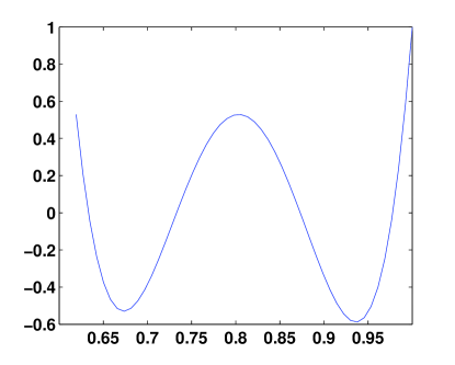
(a) SDP polynomial filter $p_{k}(\lambda),~{}\lambda_{\min}\leq\lambda\leq 1$

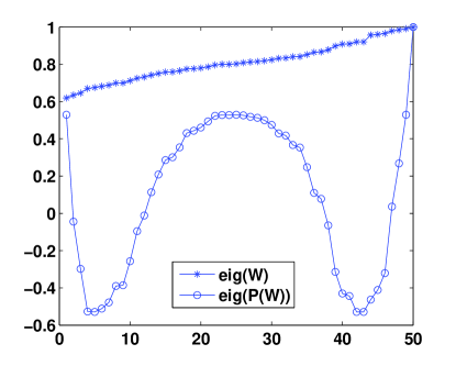
(b) Effect on the spectrum $\lambda(W)$

Figure 2: Effect of polynomial filtering on the spectrum of the Maximum-degree matrix of eq. (24).

We illustrate first the effect of polynomial filtering on the spectrum of $W$. We build a network of $n=50$ sensors and we apply polynomial filtering on the Maximum-degree weight matrix $W$, given in (24). We use $k=4$ and we solve the optimization problem OPT2 using the Maximum-degree matrix $W$ as input. Figure 2(a) shows the obtained polynomial filter $p_{k}(\lambda)$, when $\lambda\in[\lambda_{\min}(W),1]$. Next, we apply the polynomial on $W$ and Figure 2(b) shows the spectrum of $W$ before (star-solid line) and after (circle-solid line) polynomial filtering, versus the vector index. Observe that polynomial filtering dramatically increases the spectral gap $|1-\lambda_{2}|$, which further leads to accelerating the distributed consensus, as we show in the simulations that follow.

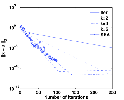
(a) SDP polynomial filtering

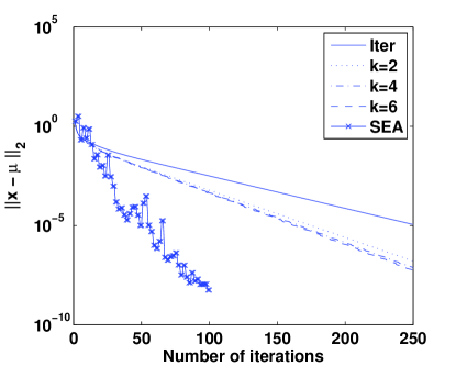
(b) Newton polynomial filtering

Figure 3: Behavior of polynomial filtering for variable degree $k$ on fixed topology using the Laplacian weight matrix.

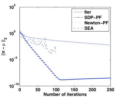
(a) Max-degree weight matrix

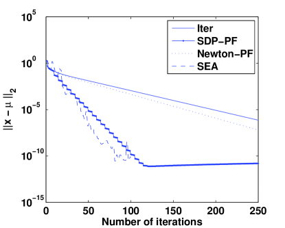
(b) Metropolis weight matrix

Figure 4: Comparison between Newton’s polynomial and SDP polynomial ($k=4$) on fixed topology.

Then we compare the performance of the different distributed consensus algorithms, with all the aforementioned weight matrices; that is, Maximum-degree, Metropolis and Laplacian weight matrices for distributed averaging. We compare both Newton’s polynomial and the SDP polynomial (obtained from the solution of OPT2) with the standard iterative method, which is based on successive iterations of eq. (3). For the sake of completeness, we also provide the results of the scalar epsilon algorithm (SEA) that uses all previous estimates [12].

First, we explore the behavior of polynomial filtering methods under variable degree $k$ from 2 to 6 with step 2. We use the Laplacian weight matrix for this experiment. Figures 3(a) and 3(b) illustrate the evolution of the absolute error $\|x_{t}-\mu\textbf{1}\|_{2}$ versus the iteration index $t$, for polynomial filtering with SDP and Newton’s polynomials respectively. We also provide the curve of the standard iterative method as a baseline. Observe first that both polynomial filtering methods outperform the standard method by exhibiting faster convergence rates, across all values of $k$. Notice also, that the degree $k$ governs the convergence rate, since larger $k$ implies more effective filtering and therefore faster convergence. Finally, the stagnation of the convergence process of the SDP polynomial filtering and large values of $k$ is due to the limited accuracy of the SDP solver.

Next, we show the results obtained with the other two weight matrices on the same sensor network. Figures 4(a) and 4(b) show the convergence behavior of all methods for the Maximum-degree and Metropolis matrices respectively. In both polynomial filtering methods we use a representative value of $k$, namely 4. Notice again that polynomial filtering accelerates the convergence of the standard iterative method (solid line). As expected, the optimal polynomial computed with SDP outperforms Newton’s polynomial, which is based on intuitive arguments only.

Finally, we can see from Figures 3 and 4 that in some cases the convergence rate is comparable for SEA and SDP polynomial filtering. Note however that the former uses all previous iterates, in contrast to the latter that uses only the $k+1$ most recent ones. Hence, the memory requirements are smaller for polynomial filtering, since they are directly driven by $k$. This moreover allows more direct control on the convergence rate, as we have seen in Fig. 3. Interestingly, we see that the convergence process is smoother with polynomial filtering, which further permits easy extension to dynamic network topologies.

5.3 Dynamic network topologies

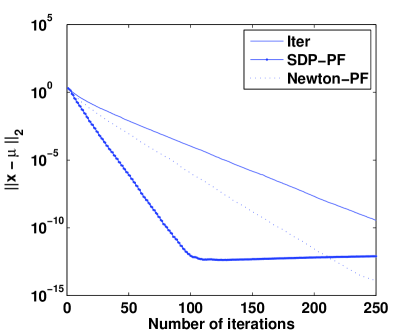
(a) $k=1$, $q=1$

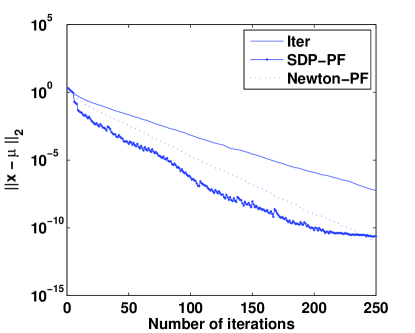
(b) $k=2$, $q=0.1$

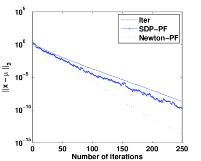
(c) $k=2$, $q=0.3$

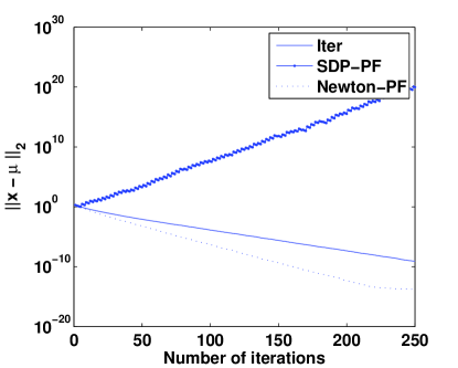
(d) $k=2$, $q=0.8$

Figure 5: Random network topology simulations. $q$ denotes the probability that the network changes at each iteration.

We study now the performance of polynomial filtering for dynamic networks topologies. We build a sequence of random networks of $n=50$ sensors, and we assume that in each iteration the network topology changes independently from the previous iterations, with probability $q$ and with probability $1-q$ it remains the same as in the previous iteration. We compare all methods for different values of the probability $q$. We use the Laplacian weight matrix (26). In the SDP polynomial filtering method, we solve the SDP program OPT4 (see Sec. 4.2). Fig. 5 shows the average performance of polynomial filtering for some representative values of the degree $k$ and the probability $q$. The average performance is computed using the median over the 100 experiments. We have not reported the performance of the SEA algorithm, since it is not robust to changes of the network topology.

Notice that when $k=1$ (i.e., each sensor uses only its current value and the right previous one) polynomial filtering accelerates the convergence over the standard method. At the same time, it stays robust to network topology changes. Also, observe that in this case, the SDP polynomial outperforms Newton’s polynomial. However, when $k=2$, the roles between the two polynomial filtering methods change as the probability $q$ increases. For instance, when $q=0.8$, the SDP method even diverges. This is expected if we think that the coefficients of Newton’s polynomial are computed using Hermite interpolation in a given interval and they do not depend on the specific realization of the underlying weight matrix. Thus, they are more generic than those of the SDP polynomial that takes $\overline{W}$ into account, and therefore less sensitive to the actual topology realization. Algorithms based on optimal polynomial filtering become inefficient in a highly dynamic network, whose topology changes very frequently.

6 Related work

Several works have studied the convergence rate of distributed consensus algorithms. In particular, the authors in [5] and [9, 10] have shown that the convergence rate depends on the second largest eigenvalue of the network weight matrix, for fixed and random networks, respectively. They both use semi-definite programs to compute the optimal weight matrix, and the optimal topology.

Other works have addressed the consensus problem, and we mention here only the most relevant ones. A. Olshevsky and J. N. Tsitsiklis in [8] propose two consensus algorithms for fixed network topologies, which build on the “agreement algorithm”. The proposed algorithms make use of spanning trees and the authors bound their worst-case convergence rate. For dynamic network topologies, they propose an algorithm which builds on a previously known distributed load balancing algorithm. In this case, the authors show that the algorithm has a polynomial bound on the convergence time ($\epsilon$-convergence).

The authors in [25] study the convergence properties of agreement over random networks following the Erdős and Rényi random graph model. According to this model, each edge of the graph exists with probability $p$, independently of other edges and the value of $p$ is the same for all edges. By agreement, we consider the case where all nodes of the graph agree on a particular value. The authors employ results from stochastic stability in order to establish convergence of agreement over random networks. Also, it is shown that the rate of convergence is governed by the expectation of an exponential factor, which involves the second smallest eigenvalue of the Laplacian of the graph.

Gossip algorithms have also been applied successfully to solving distributed averaging problems. In [15] provide convergence results on randomized gossip algorithm in both synchronous and asynchronous settings. Based on the obtained results, they optimize the network topology (edge formation probabilities) in order to maximize the convergence rate of randomized gossip. This optimization problem is also formulated as a semi-definite program (SDP). In a recent study, the authors in [20] have been able to improve the standard gossip protocols in cases where the sensors know their geometric positions. The main idea is to exploit geographic routing in order to aggregate values among random nodes that are far away in the network.

Under the same assumption of knowing the geometric positions of the sensors, the authors in [21] propose a fast consensus algorithm for geographic random graphs. In particular, they utilize location information of the sensors in order to construct a nonreversible lifted Markov chain that mixes faster than corresponding reversible chains. The main idea of lifting is to distinguish the graph nodes from the states of the Markov chain and to “split” the states into virtual states that are connected in such a way that permits faster mixing. The lifted graph is then “projected” back to the original graph, where the dynamics of the lifted Markov chain are simulated subject to the original graph topology. However, the proposed algorithm is not applicable in the case where the nodes’ geographic location is not available.

In [22] the authors propose a cluster-based distributed averaging algorithm, applicable to both fixed linear iteration and random gossiping. The induced overlay graph that is constructed by clustering the nodes is better connected relatively to the original graph; hence, the random walk on the overlay graph mixes faster than the corresponding walk on the original graph. Along the same lines, K. Jung et al. in [23], have used nonreversible lifted Markov chains to accelerate consensus. They use the lifting scheme of [24] and they propose a deterministic gossip algorithm based on a set of disjoint maximal matchings, in order to simulate the dynamics of the lifted Markov chain.

Finally, even if we have mostly considered synchronous algorithms in this paper, it is worth mentioning that the authors in [26] propose two asynchronous algorithms for distributed averaging. The first algorithm is based on blocking (that is, when two nodes update their values they block until the update has been completed) and the other algorithm drops the blocking assumption. The authors show the convergence of both algorithms under very general asynchronous timing assumptions. Moreover, the authors in [27] propose consensus propagation, which is an asynchronous distributed protocol that is a special case of belief propagation. In the case of singly-connected graphs (i.e., connected with no loops), synchronous consensus propagation converges in a number of iterations that is equal to the diameter of the graph. The authors provide convergence analysis for regular graphs.

7 Conclusions

In this paper, we proposed a polynomial filtering methodology in order to accelerate distributed average consensus in both fixed and random network topologies. The main idea of polynomial filtering is to shape the spectrum of the polynomial weight matrix in order to minimize its second largest eigenvalue and subsequently increase the convergence rate. We have constructed semi-definite programs to compute the optimal polynomial coefficients in both static and dynamic networks. Simulation results with several common weight matrices have shown that the convergence rate is much higher than for state-of-the-art algorithms in most scenarios, except in the specific case of highly dynamic networks and small memory sensors.

8 Acknowledgements

The first author would like to thank prof. Yousef Saad for the valuable and insightful discussions on polynomial filtering.

References

- [1] D. Bertsekas and J. N. Tsitsiklis, Parallel and Distributed Computation: Numerical Methods. Prentice Hall, 1989.
- [2] I. D. Schizas, A. Ribeiro, and G. B. Giannakis, “Consensus in Ad Hoc WSNs with Noisy Links - Part I: Distributed Estimation of Deterministic Signals,” IEEE Transactions on Singal Processing, vol. 56, no. 1, pp. 350–364, January 2008.
- [3] M. Rabbat, J. Haupt, A. Singh, and R. Nowak, “Decentralized compression and predistribution via randomized gossiping,” 5th ACM Int. Conf. on Information Processing in Sensor Networks (IPSN), pp. 51 – 59, April 2006.
- [4] V. D. Blondel, J. M. Hendrickx, A. Olshevsky, and J. N. Tsitsiklis, “Convergence in multiagent coordination, consensus and flocking,” IEEE Conf. on Decision and Control, and the European Control Conference, pp. 2996–3000, December 2005.
- [5] L. Xiao and S. Boyd, “Fast linear iterations for distributed averaging,” Systems and Control Letters, no. 53, pp. 65–78, February 2004.
- [6] L. Xiao, S. Boyd, and S. Lall, “A scheme for robust distributed sensor fusion based on average consensus,” Int. Conf. on Information Processing in Sensor Networks, pp. 63–70, April 2005, los Angeles.
- [7] ——, “Distributed average consensus with time-varying metropolis weights,” Automatica, June 2006, submitted.
- [8] A. Olshevsky and J. Tsitsiklis, “Convergence rates in distributed consensus and averaging,” IEEE Conference on Decision and Control, December 2006, san Diego, CA.
- [9] S. Kar and J. M. F. Moura, “Distributed average consensus in sensor networks with random link failures,” IEEE Int. Conf. on Acoustics, Speech and Signal Processing (ICASSP), April 2007.
- [10] ——, “Sensor networks with random links: Topology design for distributed consensus,” IEEE Transactions on Signal Processing, April 2007, submitted.
- [11] E. Kokiopoulou and Y. Saad, “Polynomial filtering in latent semantic indexing for information retrieval,” 27th ACM-SIGIR Conference on Research and Development in Information Retrieval, 2004.
- [12] E. Kokiopoulou and P. Frossard, “Accelarating distributed consensus using extrapolation,” IEEE Signal Processing Letters, vol. 14, no. 10, pp. 665–668, October 2007.
- [13] S. Sundaram and C. N. Hadjicostis, “Distributed consensus and linear functional calculation in networks: An observability perspective,” 6th ACM Int. Conf. on Information Processing in Sensor Networks (IPSN), April 25-27 2007.
- [14] A. Tahbaz-Salehi and A. Jadbabaie, “On consensus over random networks,” In Proceedings of 44th annual Allerton Conference on Communication, Control and Computing, pp. 1315–1321, September 2006.
- [15] B. P. S. Boyd, A. Ghosh and D. Shah, “Randomized gossip algorithms,” IEEE Transactions on Information Theory, vol. 52, pp. 2508–2530, June 2006.
- [16] S. Boyd and L. Vandenberghe, Convex Optimization. Cambridge University Press, 2004.
- [17] Y. Saad, Iterative methods for sparse linear systems, 2nd ed. SIAM, 2003.
- [18] J. F. Sturm, “Implementation of interior point methods for mixed semidefinite and second order cone optimization problems,” EconPapers 73, August 2002, Tilburg University, Center for Economic Research.
- [19] P. Gupta and P. R. Kumar, “The capacity of wireless networks,” IEEE Trans. on Information Theory, vol. 46, no. 2, pp. 388–404, March 2000.
- [20] A. Dimakis, A. D. Sarwate, and M. J. Wainwright, “Geographic gossip: Efficient averaging for sensor networks,” IEEE Trans. on Signal Processing, to appear.
- [21] W. Li and H. Dai, “Location-aided fast distributed consensus,” IEEE Transactions on Information Theory, June 2007, submitted.
- [22] ——, “Cluster-based fast distributed consensus,” IEEE Int. Conf. on Acoustics, Speech and Signal Processing (ICASSP), April 2007.
- [23] K. Jung and D. Shah, “Fast gossip via nonreversible random walk,” IEEE Information Theory Workshop (ITW), March 2006.
- [24] F. Chen, L. Lovász, and I. Pak, “Lifting markov chains to speed up mixing,” STOC ’99: Proceedings of the thirty-first annual ACM symposium on Theory of computing, pp. 275–281, 1999.
- [25] Y. Hatano and M. Mesbahi, “Agreement over random networks,” IEEE Conf. on Decision and Control, vol. 2, pp. 2010–2015, December 2004.
- [26] M. Mehyar, D. Spanos, J. Pongsajapan, S. H. Low, and R. M. Murray, “Asynchronous distributed averaging on communication networks,” IEEE/ACM Transactions on Networking, vol. 15, no. 3, pp. 512–520, June 2007.
- [27] C. C. Moallemi and B. V. Roy, “Consensus propagation,” IEEE Transactions on Information Theory, vol. 52, no. 11, pp. 4753–4766, November 2006.