Phase-coherent transport in InN nanowires of various sizes

Abstract

We investigate phase-coherent transport in InN nanowires of various diameters and lengths. The nanowires were grown by means of plasma-assisted molecular beam epitaxy. Information on the phase-coherent transport is gained by analyzing the characteristic fluctuation pattern in the magneto-conductance. For a magnetic field oriented parallel to the wire axis we found that the correlation field mainly depends on the wire cross section, while the fluctuation amplitude is governed by the wire length. In contrast, if the magnetic field is oriented perpendicularly, for wires longer than approximately 200 nm the correlation field is limited by the phase coherence length. Further insight into the orientation dependence of the correlation field is gained by measuring the conductance fluctuations at various tilt angles of the magnetic field.

Semiconductor nanowires fabricated by a bottom-up approachThelander et al. (2006); Lu and Lieber (2006); Ikejiri et al. (2007) have emerged as very interesting systems not only for the design of future nanoscale device structuresBjörk et al. (2002); Bryllert et al. (2006); Li et al. (2006) but also to address fundamental questions connected to strongly confined systems. Regarding the latter, quantum dot structures,Franceschi et al. (2003); Fasth et al. (2005); Pfund et al. (2006) single electron pumps,Fuhrer et al. (2007) or superconducting interference devicesvan Dam et al. (2006) have been realized. Many of the structures cited above were fabricated by employing III-V semiconductors, e.g. InAs or InP.Thelander et al. (2006) Apart from these more established materials, InN is particularly interesting for nanowire growth because of its low energy band gap and its high surface conductivity.Liang et al. (2002); Chang et al. (2005); Calarco and Marso (2007)

At low temperatures the transport properties of nanostructures are affected by electron interference effects, i.e. weak localization, the Aharonov–Bohm effect, or universal conductance fluctuations.Beenakker and van Houten (1991); Lin and Bird (2002) The relevant length parameter in this transport regime is the phase coherence length $l_{\phi}$, that is the length over which phase-coherent transport is maintained. In order to obtain information on $l_{\phi}$, the analysis of conductance fluctuations is a very powerful method.Umbach et al. (1984); Stone (1985); Lee and Stone (1985); Al’tshuler (1985); Lee et al. (1987); Thornton et al. (1987); Beenakker and van Houten (1988) In fact, in InAs nanowires pronounced fluctuations in the conductance have been observed and analyzed, recently.Hansen et al. (2005)

Here, we report on a detailed study of the conductance fluctuations $\delta G$ measured in InN nanowires of various sizes. Information on the phase-coherent transport is gained by analyzing the average fluctuation amplitude and the correlation field $B_{c}$. Special attention is drawn to the magnetic field orientation with respect to the wire axis, since this allowed us to change the relevant probe area for the detection of phase-coherent transport.

The InN nanowires investigated here were grown without catalyst on a Si (111) substrate by plasma-assisted MBE.Calarco and Marso (2007); Stoica et al. (2006) The measured wires had a diameter $d$ ranging from 42 nm to 130 nm. The typical wire length was 1 $\mu$m. From photoluminescence measurements an overall electron concentration of about $5\times 10^{18}$ cm^-3 was determined.Stoica et al. (2006)

For the samples used in the transport measurements, first, contact pads and adjustment markers were defined on a SiO₂-covered Si (100) wafer. Subsequently, the InN nanowires were placed on the patterned substrate and contacted individually by Ti/Au electrodes. Four wires labeled as A, B, C, and D will be discussed in detail, below. Their parameters are summarized in Table 1. In order to improve the statistics, additional wires which are not specifically labeled, were included in part of the following analysis. A micrograph of a typical contacted wire is depicted in Fig. 4 (inset).

Table 1: Dimensions and characteristic parameters of the different wires: Length $L$ (separation between the contacts), wire diameter $d$, root-mean-square of the conductance fluctuations $\mathrm{rms}(G)$, correlation field $B_{c}$. The latter two parameters were determined for $B$ parallel to the wire axis.

Wire	$L$	$d$	rms(G)	$B_{c}$
	(nm)	(nm)	($e^{2}/h$)	(T)
A	205	58	1.35	0.38
B	580	66	0.58	0.22
C	640	75	0.52	0.21
D	530	130	0.81	0.15

The transport measurements were performed in a magnetic field range from 0 to 10 T at a temperature of 0.6 K. In order to vary the angle between the wire axis and the magnetic field $B$, the samples were mounted in a rotating sample holder. The rotation axis was oriented perpendicularly to the magnetic field and to the wire axis. The magnetoresistance was measured by using a lock-in technique with an ac bias current of 30 nA.

The fluctuation pattern for nanowires with different dimensions are depicted in Fig. 1(a). Here, the normalized conductance fluctuations $\delta G$ for wires A to C comprising successively increasing diameters are plotted as a function of the magnetic field $B$. The field was oriented parallel to the wire axis. The measurements were performed up to a relatively large field of 10 T. This is justified, since even at 10 T the estimated cyclotron diameter of 70 nm just begins to become comparable to the wire diameter. The conductance variations were determined by first subtracting the typical contact resistance of $(330\pm 50)\,\Omega$, and then converting the resistance variations to conductance variations. It can clearly be seen in Fig. 1(a), that for the narrowest and shortest wire, i.e. wire A, the conductance fluctuates with a considerably larger amplitude than for the other two wires with larger diameters and length. The parameter quantifying this feature is the root-mean-square of the fluctuation amplitude $\mathrm{rms}(G)$ defined by $\sqrt{\langle\delta G^{2}\rangle}$. Here, $\langle...\rangle$ represents the average over the magnetic field. For quasi one-dimensional systems where phase coherence is maintained over the complete wire length it is expected that $\mathrm{rms}(G)$ is in the order of $e^{2}/h$.Lee and Stone (1985); Al’tshuler (1985); Lee et al. (1987) As one can infer from Table 1, for the shortest nanowire, i.e. wire A, $\mathrm{rms}(G)$ falls within this limit. For the other two wires the $\mathrm{rms}(G)$ values are smaller than $e^{2}/h$ (cf. Table 1). Thus, for these wires it can be concluded that the phase coherence length $l_{\phi}$, is smaller than the wire length $L$.

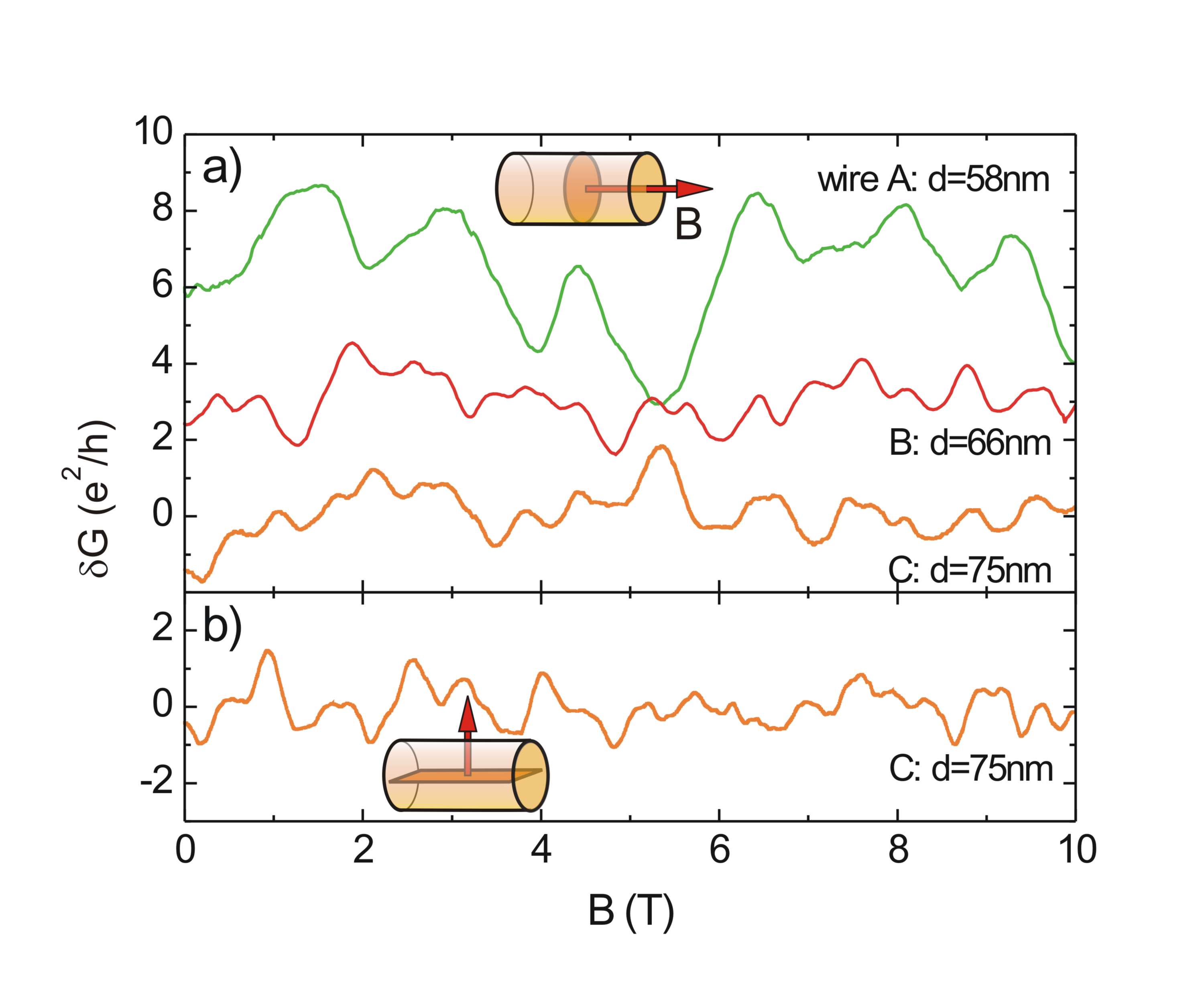
Figure 1: (a) Conductance fluctuations normalized to $e^{2}/h$ for wires with different length and diameter. The curves are offset for clarity. As illustrated by the sketch, the magnetic field is axially oriented. (b) Conductance fluctuations of wire C with a magnetic field oriented perpendicularly to the wire axis.

Beside $\mathrm{rms}(G)$, another important parameter is the correlation field $B_{c}$, quantifying on which field scale the conductance fluctuations take place. The correlation field is extracted from the autocorrelation function of $\delta G$ defined by $F(\Delta B)=\langle\delta G(B+\Delta B)\delta G(B)\rangle$.Lee et al. (1987) The magnetic field corresponding to half maximum of the autocorrelation function $F(B_{c})=\frac{1}{2}F(0)$ defines $B_{c}$. The $B_{c}$ values of the measurements shown in Fig. 1 are listed in Table 1. Obviously, for wire A, which has the smallest diameter, one finds the largest value of $B_{c}$. In a semiclassical approach it is expected that $B_{c}$ is inversely proportional to the maximum area $A_{\phi}$ perpendicular to $B$ which is enclosed phase-coherently:Lee and Stone (1985); Lee et al. (1987); Beenakker and van Houten (1988)

$$B_{c}=\alpha\frac{\Phi_{0}}{A_{\phi}}\;.$$ (1)

Here, $\alpha$ is a constant in the order of one and $\Phi_{0}=h/e$ the magnetic flux quantum. As long as phase coherence is maintained along the complete circumference, $A_{\phi}$ is equal to the wire cross section $\pi d^{2}/4$ and thus one expects $B_{c}\propto 1/d^{2}$. The $B_{c}$ values given in Table 1 follow this trend, i.e. becoming smaller for increasing diameter $d$. As can be recognized in Fig. 2 (inset), $F(\Delta B)$ also shows negative values at larger $\Delta B$. This behavior can be attributed to the limited number of modes in the wires, as it was observed previously for small size semiconductor structures.Jalabert et al. (1990); Bird et al. (1996) However, as discussed by Jalabert et al.Jalabert et al. (1990), at small fields $F(\Delta B)$ and thus $B_{c}$ being calculated fully quantum mechanically correspond well to the semiclassical approximation.

In order to elucidate the dependence of $B_{c}$ on the wire diameter in more detail, a larger number of wires was measured. As can be seen in Fig. 2(a), $B_{c}$ systematically decreases with $d$. Leaving out wire D which has the largest diameter, the decrease of $B_{c}$ is well described by a $1/d^{2}$-dependence. As mentioned above, for short wires ($L\approx 200$ nm) we found that phase coherence is maintained over the complete length. This length corresponds to a circumference of a wire with a diameter of about 64 nm. Except of wire D, $d$ is in the order of that value, so that one can expect that phase coherence is maintained within the complete cross section. For the parameter $\alpha$ we found a value of 0.24, which is by a factor of 4 smaller than the theoretically expected value of 0.95.Beenakker and van Houten (1988) Choosing $\alpha=0.95$ would result in lower bound values of $B_{c}$ being larger than all corresponding experimental values, which is physically unreasonable. We attribute the discrepancy to the different geometrical situation, i.e. for the latter a confined two-dimensional electron gas with a perpendicularly oriented magnetic field was considered,Beenakker and van Houten (1988) while in our case the field is oriented parallel to the wire axis. In addition, an inhomogeneous carrier distribution within the cross section, e.g. due to a carrier accumulation at the surface,Mahboob et al. (2004) can also result in a disagreement between experiment and theoretical model. As can be seen in Fig. 2(a) (inset), the data point of the wire with the largest diameter of 130 nm, i.e. wire D, is found above the calculated curve. This indicates that presumably for this sample, $A_{\phi}$ is slightly smaller than the wire cross section.

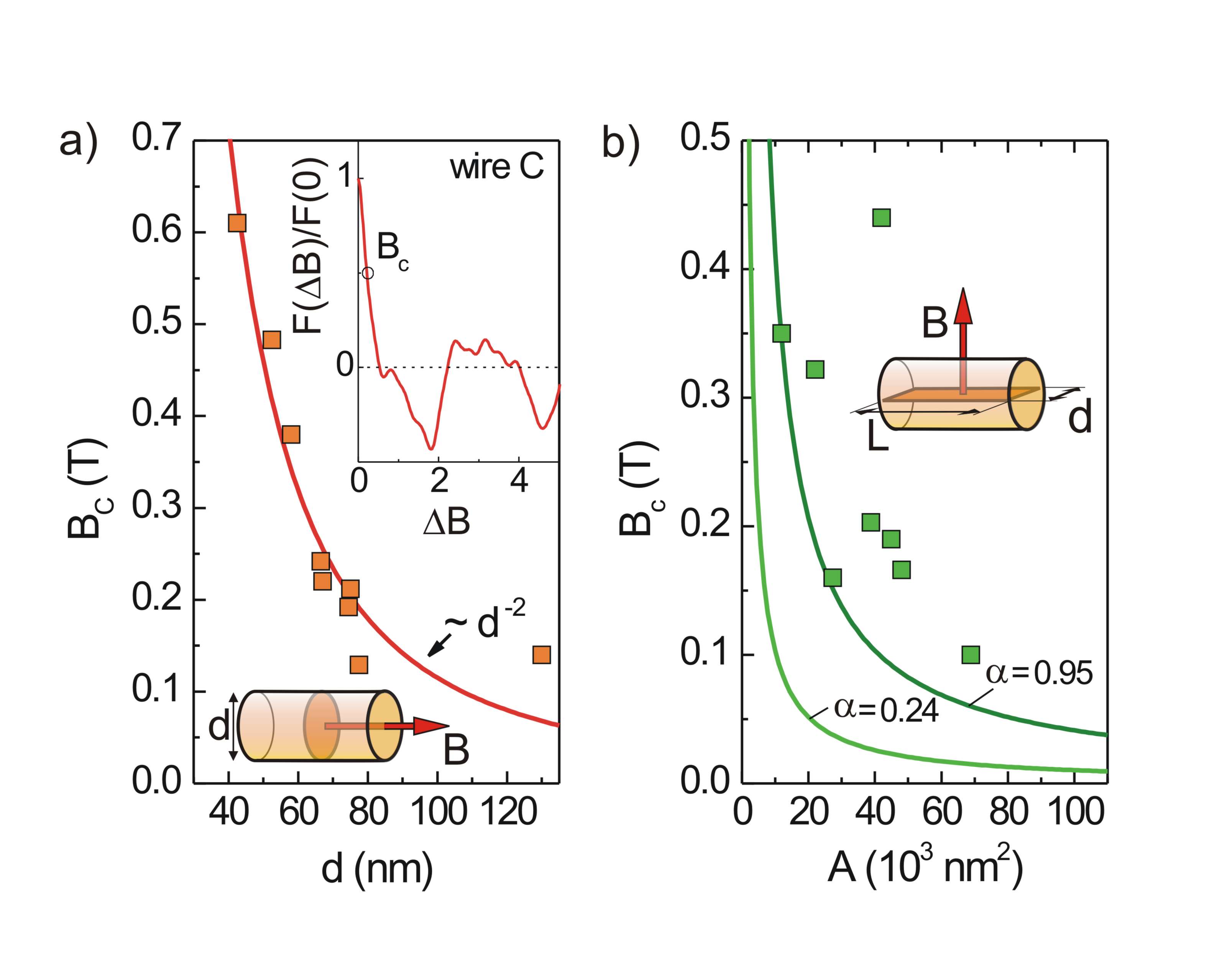
Figure 2: (a) Correlation field $B_{c}$ as a function of the wire diameter $d$. As illustrated in the schematics the magnetic field $B$ was oriented axially. The solid lines corresponds to the calculated correlation field. The inset shows $F(\Delta B)/F(0)$ for wire C. (b) $B_{c}$ as a function of the maximum area $A=Ld$ (see schematics) of the wire. The magnetic field is oriented perpendicular to the wire axis. The solid lines represents the calculated lower boundary correlation fields assuming $\alpha=0.95$ and 0.24, respectively.

Next, we will focus on measurements of $\delta G$ with a magnetic field oriented perpendicular to the wire axis. As a typical example, $\delta G$ of wire C is shown in Fig. 1(b). Here, a correlation field of $0.17$ T was extracted, which is smaller than the value of corresponding measurements with $B$ parallel to the wire axis [c.f. Fig. 1(a) and Table 1]. The smaller value of $B_{c}$ can be attributed to the effect that now the relevant area for magnetic flux-induced interference effects is no longer limited by the relatively small circular cross section but rather by a larger area within the rectangle defined by $L$ and $d$, as illustrated by the schematics in Fig. 2(b).

In Fig. 2(b) the $B_{c}$ values of various wires are plotted as a function of the maximum area $A_{max}=Ld$ penetrated by the magnetic field. As a reference, the calculated curve using Eq. (1) and assuming $A_{\phi}=A_{max}$ are also plotted. It can be seen that the $B_{c}$ values of two wires with small areas, including wire A, match to the theoretically expected ones if one takes $\alpha=0.95$, as given by Beenakker and van Houten.Beenakker and van Houten (1988) This corresponds to the case of phase-coherent transport across the complete wire, as it was, in case of wire A, already concluded from the $\mathrm{rms}(G)$ analysis. For all other wires the $B_{c}$ values are above the theoretically expected curve, corresponding to the case $A_{\phi}<A_{max}$. At this point, one might argue that for $B$ oriented along the wire axis a better agreement is found for $\alpha=0.24$. However, as can be seen in Fig. 2(b), if one assumes $\alpha=0.24$ all experimental values are above the calculated curve, i.e. $A_{\phi}<A_{max}$. This does not agree with the observation that for short wires $\mathrm{rms}(G)$ is in the order of $e^{2}/h$. We attribute the difference between the appropriate $\alpha$ values for different field orientations to the different character of the relevant area penetrated by the magnetic flux, e.g. due to carrier accumulation at the surface.

Beside $B_{c}$ we also analyzed the fluctuation amplitude for five different wires with $B$ oriented perpendicular to the wire axis. Only wires with comparable diameters of ($75\pm 5$) nm were chosen, here. It can be seen in Fig. 3 that $\mathrm{rms}(G)$ tends to decrease with increasing wire length $L$.

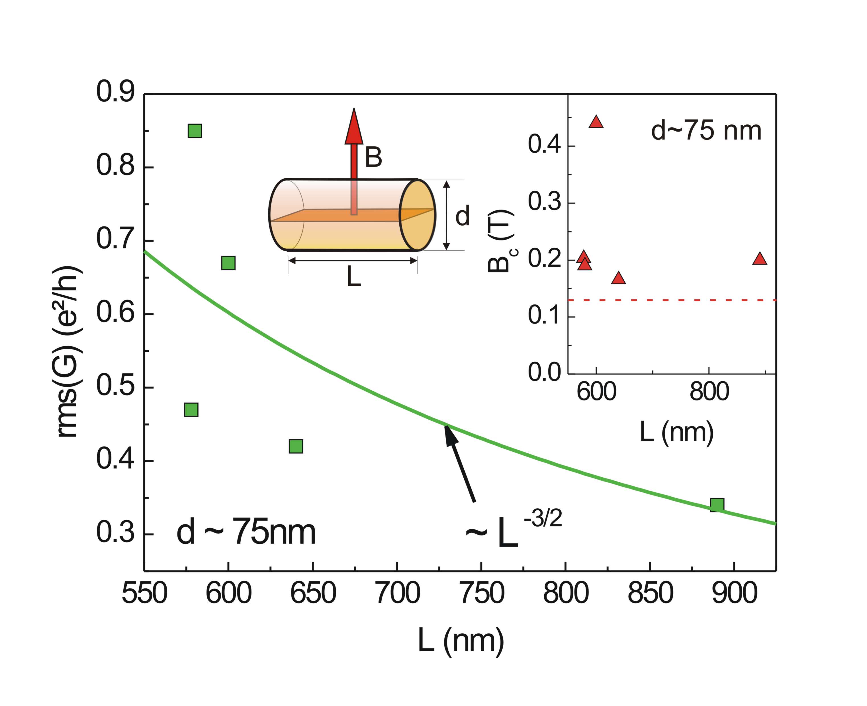
Figure 3: $\mathrm{rms}(G)$ for wires with a diameter of $(75\pm 5)$ nm as a function of wire length $L$ (square). The magnetic field is oriented perpendicular to the wire axis. The calculated decrease of $\mathrm{rms}(G)$ proportional to $L^{-3/2}$ is plotted as solid line. The inset shows $B_{c}$ vs. $L$ for wires with $d\approx 75$ nm. The dashed line corresponds to the calculated value of $B_{c}$ assuming $l_{\phi}=430$ nm.

From the previous discussion of $B_{c}$ it was concluded that for long wires, as it is the case here, $l_{\phi}<L$. In this regime $\mathrm{rms}(G)$ is expected to depend on $L$ asLee et al. (1987); Beenakker and van Houten (1988)

$$\mathrm{rms}(G)=\beta\frac{e^{2}}{h}\left(\frac{l_{\phi}}{L}\right)^{3/2}\;,$$ (2)

with $\beta$ in the order of one. The above expression is valid as long as the thermal diffusion length $l_{T}=\sqrt{\hbar\mathcal{D}/k_{B}T}$, is larger than $l_{\phi}$. Here, $\mathcal{D}$ is the diffusion constant. From our transport data we estimated $l_{T}\approx 600$ nm at $T=0.6$ K. As can be seen in Fig. 3, the available experimental data points roughly follow the trend of the calculated curve using Eq. (2) and assuming $l_{\phi}=430$ nm and $\beta=1$. For the limit $l_{\phi}<L$, a correlation field according to $B_{c}=0.95\Phi_{0}/d\l_{\phi}$ is expected.Lee et al. (1987) As confirmed in Fig. 2(b), most experimental values of $B_{c}$ are close to the calculated one.

If one compares the $\mathrm{rms}(G)$ values for wires with $d\approx 75$ nm and $B$ oriented axially (not shown here) with the corresponding values for $B$ oriented perpendicularly, one finds, that both are in the same range. Thus it can be concluded that the fluctuation amplitude does not significantly depend on the magnetic field orientation. This is in contrast to the correlation field, where one finds a systematic dependence on the orientation of $B$.

In order to discuss the latter aspect in more detail the correlation field was studied for various tilt angles $\theta$ of the magnetic field. Figure 4 shows $B_{c}$ of sample D if $\theta$ is increased from $0^{\circ}$ to $90^{\circ}$. The inset in Fig. 4 illustrates how $\theta$ is defined.

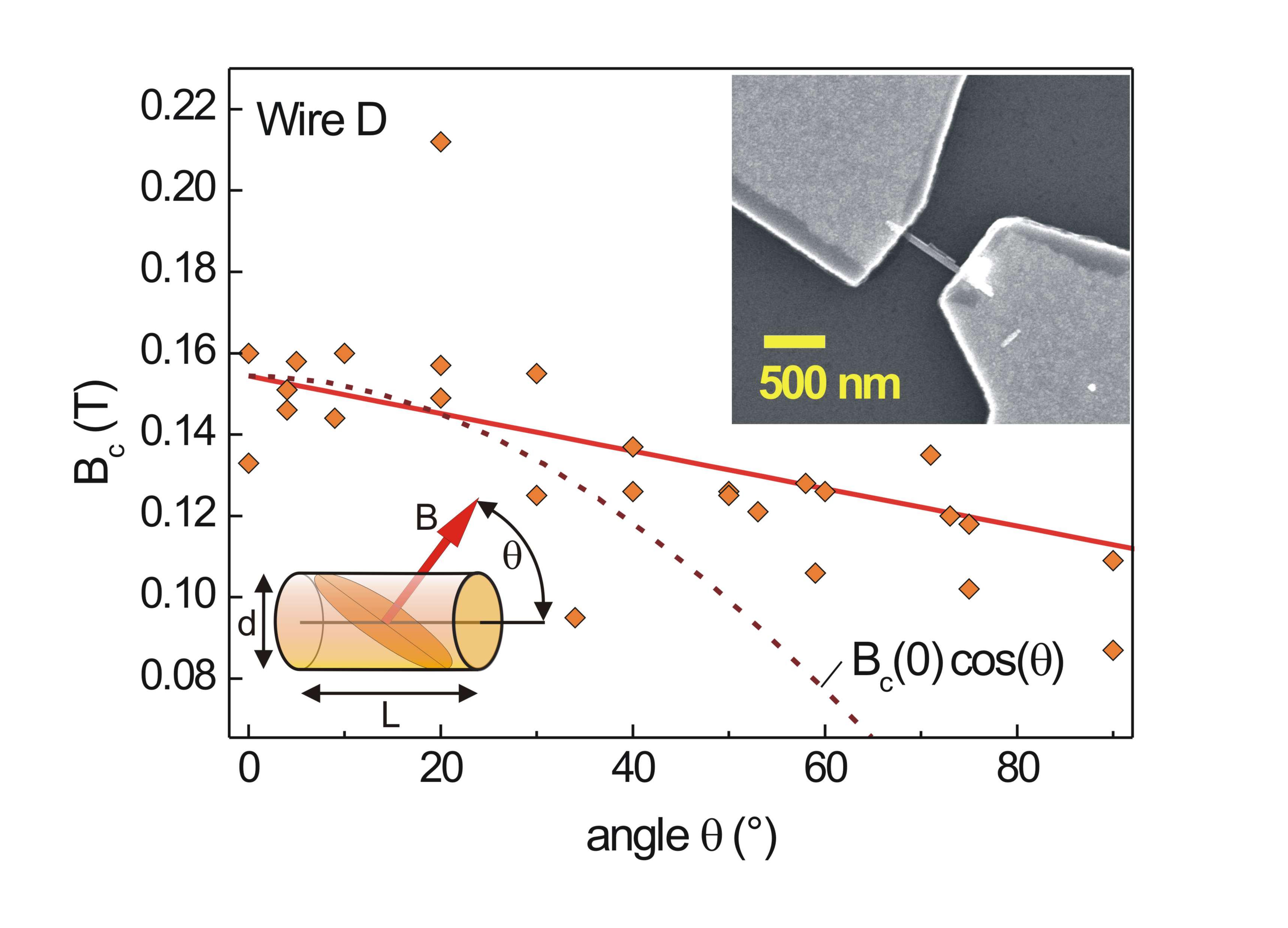
Figure 4: Correlation field $B_{c}$ of wire D as a function of the angle $\theta$ between the wire axis and $B$. The solid line represents a linear fit. The broken line corresponds to the theoretically expected $B_{c}$ if phase-coherent transport is assumed in the complete wire. The left-hand-side inset shows a schematics of the geometrical situation. The right-hand-side inset shows a micrograph of a 580-nm-long wire with a diameter of 66 nm.

Obviously, $B_{c}$ decreases with increasing tilt angle $\theta$. As explained above, the value of $B_{c}$ is a measure of the maximum area normal to $B$, which is enclosed phase-coherently by the electron waves in the wire [see Fig. 4 (schematics)]. As long as $\theta\leq\arctan(L/d)$, this maximum area is given by $A(\theta)=\pi d^{2}/4\cos{\theta}$. The expected $\theta$-dependence of the correlation field is then given by $B_{c}(\theta)$=$B_{c}(0)\cos(\theta)$, with $B_{c}(0)$ the correlation field at $\theta=0$. As can be seen in Fig. 4, the calculated correlation field $B_{c}$, corresponding to fully phase-coherent transport, decreases much faster with increasing $\theta$ than the experimentally determined values. The experimental situation is better described by a linear decrease. As it was discussed above, at $\theta=0$ one can assume that the area enclosed phase-coherently is equal to $A(0)$. However, if the tilt angle is increased the maximum wire cross section $A(\theta)$ presumably becomes larger than $A_{\phi}$, resulting in a much smaller decrease of $B_{c}$ than theoretically expected for fully phase-coherent transport. In addition, as pointed out above, the different tilt angles result in an angle-dependent parameter $\alpha$. This is supported by the measurements of $B_{c}$ for $B$ parallel and perpendicular to the wire axis, where different values for $\alpha$ were determined, respectively.

In conclusion, the conductance fluctuations of InN nanowires with various lengths and diameters were investigated. We found that for an axially oriented magnetic field the correlation field $B_{c}$ and thus the area where phase-coherent transport is maintained is limited by the wire cross section perpendicular to $B$. In contrast, $\mathrm{rms}(G)$ decreases with the wire length, since this quantity also depends on the propagation of the electron waves along the wire axis. If the magnetic field is oriented perpendicularly we found that for long wires $B_{c}$ is limited by $l_{\phi}$ rather than by the length $L$. Our investigations demonstrate that phase-coherent transport can be maintained in InN nanowires, which is an important prerequisite for the design of quantum device structures based on this material system.

References

- Thelander et al. (2006) C. Thelander, P. Agarwal, S. Brongersma, J. Eymery, L. Feiner, A. Forchel, M. Scheffler, W. Riess, B. Ohlsson, U. Gösele, et al., Materials Today 9, 28 (2006).
- Lu and Lieber (2006) W. Lu and C. M. Lieber, J. Phys. D: Appl. Phys. 39, R387 (2006).
- Ikejiri et al. (2007) K. Ikejiri, J. Noborisaka, S. Hara, J. Motohisa, and T. Fukui, J. Cryst. Growth 298, 616 (2007).
- Björk et al. (2002) M. T. Björk, B. J. Ohlsson, C. Thelander, A. I. Persson, K. Deppert, L. R. Wallenberg, and L. Samuelson, Appl. Phys. Lett. 81, 4458 (2002).
- Bryllert et al. (2006) T. Bryllert, L.-E. Wernersson, T. Lowgren, and L. Samuelson, Nanotechnology 17, 227 (2006).
- Li et al. (2006) Y. Li, J. Xiang, F. Qian, S. Gradecak, Y. Wu, H. Yan, D. Blom, and C. M. Lieber, Nano Letters 6 (2006).
- Franceschi et al. (2003) S. D. Franceschi, J. A. van Dam, E. P. A. M. Bakkers, L. Feiner, L. Gurevich, and L. P. Kouwenhoven, Appl. Phys. Lett. 83, 344 (2003).
- Fasth et al. (2005) C. Fasth, A. Fuhrer, M. T. Bjork, and L. Samuelson, Nanoletters 5, 1487 (2005).
- Pfund et al. (2006) A. Pfund, I. Shorubalko, R. Leturcq, and K. Ensslin, Appl. Phys. Lett. 89, 252106 (2006).
- Fuhrer et al. (2007) A. Fuhrer, C. Fasth, and L. Samuelson, Appl. Phys. Lett. 91, 052109 (2007).
- van Dam et al. (2006) J. A. van Dam, Y. V. Nazarov, E. P. A. M. Bakkers, S. D. Franceschi, and L. P. Kouwenhoven, Nature 442, 667 (2006).
- Liang et al. (2002) C. H. Liang, L. C. Chen, J. S. Hwang, K. H. Chen, Y. T. Hung, and Y. F. Chen, Appl. Phys. Lett. 81, 22 (2002).
- Chang et al. (2005) C.-Y. Chang, G.-C. Chi, W.-M. Wang, L.-C. Chen, K.-H. Chen, F. Ren, and S. J. Pearton, Appl. Phys. Lett. 87, 093112 (2005).
- Calarco and Marso (2007) R. Calarco and M. Marso, Appl. Phys. A 87, 499 (2007).
- Beenakker and van Houten (1991) C. W. J. Beenakker and H. van Houten, in Solid State Physics, edited by H. Ehrenreich and D. Turnbull (Academic, New York, 1991), vol. 44, p. 1.
- Lin and Bird (2002) J. J. Lin and J. P. Bird, J. Phys.: Cond. Mat. 14, R501 (2002).
- Umbach et al. (1984) C. P. Umbach, S. Washburn, R. B. Laibowitz, and R. A. Webb, Phys. Rev. B 30, 4048 (1984).
- Stone (1985) A. D. Stone, Phys. Rev. Lett. 54, 2692 (1985).
- Lee and Stone (1985) P. A. Lee and A. D. Stone, Phys. Rev. Lett. 55, 1622 (1985).
- Al’tshuler (1985) B. Al’tshuler, Pis’ma Zh. Eksp. Teo. Fiz. [JETP Lett. 41, 648-651 (1985)] 41, 530 (1985).
- Lee et al. (1987) P. A. Lee, A. D. Stone, and H. Fukuyama, Phys. Rev. B 35, 1039 (1987).
- Thornton et al. (1987) T. J. Thornton, M. Pepper, H. Ahmed, G. J. Davies, and D. Andrews, Phys. Rev. B 36, 4514 (1987).
- Beenakker and van Houten (1988) C. W. J. Beenakker and H. van Houten, Phys. Rev. B 37, 6544 (1988).
- Hansen et al. (2005) A. E. Hansen, M. T. Börk, C. Fasth, C. Thelander, and L. Samuelson, Phys. Rev. B 71, 205328 (2005).
- Stoica et al. (2006) T. Stoica, R. J. Meijers, R. Calarco, T. Richter, E. Sutter, and H. Lüth, Nano Lett. 6, 1541 (2006).
- Jalabert et al. (1990) R. A. Jalabert, H. U. Baranger, and A. D. Stone, Phys. Rev. Lett. 65, 2442 (1990).
- Bird et al. (1996) J. P. Bird, D. K. Ferry, R. Akis, Y. Ochiai, K. Ishsibashi, Y. Aoyagi, and T. Sugano, Europhys. Lett. 35, 529 (1996).
- Mahboob et al. (2004) I. Mahboob, T. D. Veal, C. F. McConville, H. Lu, and W. J. Schaff, Phys. Rev. Lett. 92, 036804 (2004).