Multi-wavelength observations
of a nearby multi-phase interstellar cloud

Abstract

Aims. High-resolution spectroscopic observations (UV HST/STIS and optical) are used to characterize the physical state and velocity structure of the multiphase interstellar medium seen towards the nearby ($170\,$pc) star HD 102065. The star is located behind the tail of a cometary-shaped, infrared cirrus-cloud, in the area of interaction between the Sco-Cen OB association and the Local Bubble.

Methods. We analyze interstellar components present along the line of sight by fitting multiple transitions from a group of species all at once. We identify four groups of species: (1) molecules (CO, CH, CH⁺), (2) atoms (C i, S i, Fe i) with ionization potential lower than H i, (3) neutral and low-ionized states of atoms (Mg i, Mg ii, Mn ii, P ii, Ni ii, C ii, N i and O i) with ionization potential larger than H i and (4) highly-ionized atoms (Si iii, C iv, Si iv). The absorption spectra are complemented by H i, CO and C ii emission-line spectra, H₂ column-densities derived from FUSE spectra, and IRAS images.

Results. Gas components of a wide range of temperatures and ionization states are detected along the line of sight. Most of the hydrogen column-density is in cold, diffuse, molecular gas at low LSR velocity. This gas is mixed with traces of warmer molecular gas traced by H₂ in the $J>2$ levels, in which the observed CH⁺ must be formed.

We also identify three distinct components of warm gas at negative velocities down to $-20{\rm\,km\,{s}^{-1}}$. The temperature and gas excitation are shown to increase with increasing velocity shift from the bulk of the gas.

Hot gas at temperatures of several $10^{5}$ K is detected in the most negative velocity component in the highly-ionized specie. This hot gas is also detected in very strong lines of less-ionized species (Mg ii, Si ii^∗ and C ii^∗) for which the bulk of the gas is cooler.

Conclusions. We relate the observational results to evidence for dynamical impact of the Sco-Cen stellar association on the nearby interstellar medium. We propose a scenario where the infrared cirrus cloud has been hit a few $10^{5}\,$yr ago by a supernova blast wave originating from the Lower Centaurus Crux group of the Sco-Cen association.

The observations provide detailed information on the interplay between ISM phases in relation with the origin of the Local and Loop I bubbles.

1 Introduction

Astronomical observations provide multiple perspectives on the interstellar matter, gas and dust, that are rarely gathered together to study the relation between interstellar-medium phases. It is the ambition of this paper to present such a study on gas and dust observed in the direction of the nearby (170 pc), lightly reddened (E(B-V) = 0.17), B9IV star HD 102065 in Chamaeleon (Table 1). In IRAS images, the infrared cirrus (Dcld 300.2-16.9) seen in the foreground of HD 102065 has a prominent cometary shape and an unusually blue IRAS colors (high 12 and $25\,\mu$m to $100\,\mu$m brightness ratio), indicative of a large abundance of small stochastically-heated dust particles (Boulanger et al. 1990). We hereafter refer to it as the Blue Cloud in reference to its blue infrared colors. While the main Chamaeleon clouds have a comparable extent in CO surveys as in IRAS images, only the center of the Blue Cloud head is detected in CO (Boulanger et al., 1998; Mizuno et al., 2001). Boulanger et al. estimate that only 10% of the cloud mass is seen in CO emission. On larger angular scales, HD 102065 lies within the sky area where various evidences for an interaction between the Scorpius-Centaurus (Sco-Cen) OB association and the Local Bubble have been gathered from H i observations (de Geus 1992), the X-ray ROSAT survey (Egger and Aschenbach 1995) and optical absorption-line spectroscopy (Corradi et al. 2004).

HD 102065 is located at the same Galactic longitude and slightly lower Galactic latitude than the Lower Centaurus Crux (LCC) group of the Sco-Cen association. Hipparcos positions, proper motions, and parallaxes have been used to show that the LCC and the Upper Centaurus Lupus (UCL) group of stars, presently located within the Loop I bubble at a distance of $\sim 120\,$pc, were located closer to the Sun $5-7\,$Myr ago. In two independent works (Maiz-Apellaniz 2001 and Berghöfer and Breitschwerdt 2002), this information was used to relate the origin of the Local Bubble to the $\sim 20$ supernovae explosions associated with the LCC and UCL groups that are estimated to have occurred in the last 10 Myr. The structure and physical state of the interstellar medium seen in direction of the Sco-Cen association should reflect the action of the supernovae explosions powering and progressively shredding, and spreading away the stars’ parent cloud. This scenario has been introduced into a numerical simulation based on the supernovae-driven ISM model of de Avillez (2000) by Breitschwerdt and de Avillez (2006). In the reproduction of the local interstellar medium generated by this simulation (Figure 1 in Breitschwerdt and de Avillez), HD 102065 is located within the Loop I bubble and the line of sight to the star crosses the shell that provides separation from the Local Bubble.

Observations characterizing the gas and the dust along the line of sight to HD102065 have been presented in earlier publications (Boulanger, Prevot & Gry, 1994 ; Gry et al, 1998). Unlike most early-type stars observed in UV spectroscopy, the position of HD 102065 corresponds to no enhancement in IRAS emission, implying that the matter responsible for absorption is not heated by the star (Boulanger et al., 1994). The extinction curve produced using IUE low-resolution spectroscopy, shows a strong 220 nm bump and a weak far-UV rise (Boulanger et al., 1994). Moderate-resolution spectroscopy ($\lambda/\Delta\lambda=20\,000$) acquired by FUSE, detected molecular hydrogen absorption lines. These observations showed that ${\rm{H}}_{2}$ at a temperature of $\sim\,60\,$K is the dominant state of hydrogen along the line of sight to HD 102065. The presence of a smaller amount of warmer ${\rm{H}_{2}}$ (a few 100 K) was inferred from the H₂ excitation (Gry et al., 2002). HD 102065 was also observed using the Goddard High Resolution Spectrometer (GHRS) on the Hubble Space Telescope (HST). These observations revealed the presence of high, negative-velocity gas with unusually high ${\rm{Si\leavevmode\nobreak\ {\sc ii}}}$ excitation that was seen as the signature of the dissipation of a large amount of kinetic energy (Gry et al., 1998).

	HD 102065
$\alpha$ (2000)	11 43 37.87
$\delta$ (2000)	-80 28 59.4
l (2000)	300.02∘
b (2000)	-18.00∘
Sp. Type	B9IV
d (pc)	170
E(B-V)	$0.17\pm 0.04$
$A_{v}$	$0.67\pm 0.12$
$R_{v}$	$3.9\pm 0.4$
N(${\rm{H}_{2}}$,J=0) (${\rm{cm}^{-2}}$)	$2.0\pm 0.2\>10^{20}$
N(${\rm{H}_{2}}$,J=1) (${\rm{cm}^{-2}}$)	$1.4\pm 0.1\>10^{20}$
N(${\rm{H}}_{2}$,J=2) (${\rm{cm}}^{-2}$)	$2.5-2.6\,10^{18}$
N(${\rm{H}_{2}}$,J=3) (${\rm{cm}^{-2}}$)	$1.1-3.1\,10^{17}$
N(${\rm{H}_{2}}$,J=4) (${\rm{cm}^{-2}}$)	$0.6-5.6\,10^{16}$
N(${\rm{H}}_{2}$,J=5) (${\rm{cm}}^{-2}$)	$0.45-1.2\,10^{15}$
NH (${\rm{cm}}^{-2}$)	$9.9\>10^{20}$
$f=2N(H_{2})/N_{H}$	$0.69\pm 0.12$

Table 1: HD 102065 “fact sheet”. $A_{v}$ is the visible extinction, E(B-V) is the color index (Boulanger et al., 1994). ${\rm{H}_{2}}$ column densities from (Gry et al., 2002). The total column density (N_H = N(H) + 2 N(H₂)) has been derived from E(B-V).

A number of questions remain unanswered. Why is the small dust abundance enhanced in the Blue Cloud, which, from the FUSE and optical spectroscopy, appears to be a typical diffuse molecular cloud? How was the negative-velocity gas accelerated? Are the low and negative-velocity gas physically connected? More generally, how can the data be interpreted within the present understanding of the interaction between the Loop I and the Local bubbles?

In this paper, we present high-resolution ($R=100\,000$) UV spectr,a obtained using the HST Imaging Spectrograph (STIS) complemented by optical absorption spectra, and CO and H i emission spectroscopy (Sections 2 and 3). These data improve previous observations in spectral resolution and spectral coverage. The multi-wavelength spectra are used to describe the physical state and velocity structure of the multiple gas components observed along the line of sight (Section 4). In Section 5, we discuss the cool, low-velocity gas, and in Section 6, we relate the observational results to evidence for dynamical interaction between the Sco-Cen stars and the nearby interstellar medium, and discuss the possible interplay between the multiple components. The main conclusions of this paper are gathered in Section 7.

Element	Wavelength (Å)	f-value						Element	Wavelength (Å)	f-value
${\rm{C\leavevmode\nobreak\ {\sc I}}}$	1276.4822	0.449 $10^{-2}$						${\rm{Fe\leavevmode\nobreak\ {\sc II}}}$	1608.4510	0.58 $10^{-1}$
${\rm{C\leavevmode\nobreak\ {\sc I}}}$	1280.1353	0.229 $10^{-1}$						${\rm{Fe\leavevmode\nobreak\ {\sc II}}}$	1611.2004	0.136 $10^{-2}$
${\rm{C\leavevmode\nobreak\ {\sc I}}}$	1328.8333	0.631 $10^{-1}$						${\rm{Fe\leavevmode\nobreak\ {\sc II}}}$	2586.6499	0.691 $10^{-1}$
${\rm{C\leavevmode\nobreak\ {\sc I}}}$	1560.3092	0.128 $10^{-1}$						${\rm{Fe\leavevmode\nobreak\ {\sc II}}}$	2382.7651	0.320
${\rm{C\leavevmode\nobreak\ {\sc I}}}$	1656.9283	0.140 $10^{0}$						${\rm{Fe\leavevmode\nobreak\ {\sc II}}}$	2600.1729	0.239
${\rm{C\leavevmode\nobreak\ {\sc I}}^{*}}$	1260.9261	0.135 $10^{-1}$						${\rm{Mn\leavevmode\nobreak\ {\sc II}}}$	2576.8770	0.361
${\rm{C\leavevmode\nobreak\ {\sc I}}^{*}}$	1260.9961	0.105 $10^{-1}$						${\rm{Mn\leavevmode\nobreak\ {\sc II}}}$	2594.4990	0.280
${\rm{C\leavevmode\nobreak\ {\sc I}}^{*}}$	1261.1224	0.147 $10^{-1}$						${\rm{Mn\leavevmode\nobreak\ {\sc II}}}$	2606.4619	0.198
${\rm{C\leavevmode\nobreak\ {\sc I}}^{*}}$	1277.2827	0.705 $10^{-1}$						${\rm{Mg\leavevmode\nobreak\ {\sc II}}}$	1239.9253	0.617 $10^{-3}$
${\rm{C\leavevmode\nobreak\ {\sc I}}^{*}}$	1277.5131	0.223 $10^{-1}$						${\rm{Mg\leavevmode\nobreak\ {\sc II}}}$	1240.3947	0.354 $10^{-3}$
${\rm{C\leavevmode\nobreak\ {\sc I}}^{*}}$	1280.5975	0.674 $10^{-2}$						${\rm{Mg\leavevmode\nobreak\ {\sc II}}}$	2803.5305	0.306
${\rm{C\leavevmode\nobreak\ {\sc I}}^{*}}$	1279.8907	0.126 $10^{-1}$						${\rm{Mg\leavevmode\nobreak\ {\sc II}}}$	2796.3518	0.615
${\rm{C\leavevmode\nobreak\ {\sc I}}^{*}}$	1656.2672	0.558 $10^{-1}$						${\rm{S\leavevmode\nobreak\ {\sc II}}}$	1250.5840	0.543 $10^{-2}$
${\rm{C\leavevmode\nobreak\ {\sc I}}^{*}}$	1657.3792	0.356 $10^{-1}$						${\rm{S\leavevmode\nobreak\ {\sc II}}}$	1253.8110	0.109 $10^{-1}$
${\rm{C\leavevmode\nobreak\ {\sc I}}^{*}}$	1657.9071	0.471 $10^{-1}$						${\rm{S\leavevmode\nobreak\ {\sc II}}}$	1259.5190	0.166 $10^{-1}$
${\rm{C\leavevmode\nobreak\ {\sc I}}}^{**}$	1277.5500	0.791 $10^{-1}$						${\rm{P\leavevmode\nobreak\ {\sc II}}}$	1301.8743	0.127 $10^{-1}$
${\rm{C\leavevmode\nobreak\ {\sc I}}^{**}}$	1329.5775	0.474 $10^{-1}$						${\rm{P\leavevmode\nobreak\ {\sc II}}}$	1532.5330	0.303 $10^{-2}$
${\rm{C\leavevmode\nobreak\ {\sc I}}^{**}}$	1329.6003	0.159 $10^{-1}$						${\rm{C\leavevmode\nobreak\ {\sc I}I}}$	1334.5323	0.128
${\rm{C\leavevmode\nobreak\ {\sc I}}^{**}}$	1561.4377	0.107 $10^{-1}$						${\rm{C\leavevmode\nobreak\ {\sc II}}^{*}}$	1335.7080	0.115
${\rm{C\leavevmode\nobreak\ {\sc I}}^{**}}$	1657.0081	0.104 $10^{-1}$						${\rm{\rm{Si\leavevmode\nobreak\ {\sc II}}}}$	1304.3702	0.917 $10^{-1}$
${\rm{S\leavevmode\nobreak\ {\sc I}}}$	1295.6531	0.870 $10^{-1}$						${\rm{Si\leavevmode\nobreak\ {\sc II}}}$	1193.2897	0.585
${\rm{S\leavevmode\nobreak\ {\sc I}}}$	1296.1740	0.220 $10^{-1}$						${\rm{Si\leavevmode\nobreak\ {\sc II}}}$	1260.4221	0.118 $10^{1}$
${\rm{S\leavevmode\nobreak\ {\sc I}}}$	1425.1877	0.365 $10^{-1}$						${\rm{\rm{Si\leavevmode\nobreak\ {\sc II}}}}$	1190.4158	0.293
${\rm{S\leavevmode\nobreak\ {\sc I}}}$	1473.9943	0.730 $10^{-1}$						${\rm{Si\leavevmode\nobreak\ {\sc II}}^{*}}$	1264.7377	0.106 $10^{1}$
${\rm{S\leavevmode\nobreak\ {\sc I}}}$	1474.5706	0.121 $10^{-2}$						${\rm{Si\leavevmode\nobreak\ {\sc II}}^{*}}$	1194.5002	0.730
${\rm{Fe\leavevmode\nobreak\ {\sc I}}}$	2523.6084	0.279						${\rm{Si\leavevmode\nobreak\ {\sc II}}^{*}}$	1197.3938	0.146
${\rm{Fe\leavevmode\nobreak\ {\sc I}}}$	2484.0210	0.557						${\rm{Si\leavevmode\nobreak\ {\sc II}}^{*}}$	1265.0020	0.118
${\rm{Mg\leavevmode\nobreak\ {\sc I}}}$	2852.9641	0.183 $10^{1}$						${\rm{Si\leavevmode\nobreak\ {\sc II}}^{*}}$	1309.2758	0.913 $10^{-1}$
CO A-X (2,0) :								${\rm{Si\leavevmode\nobreak\ {\sc II}}}^{*}$	1533.4321	0.131
${\rm{R(0)}}$	1477.5669	3.933 $10^{-2}$						${\rm{O\leavevmode\nobreak\ {\sc I}}}$	1302.1685	0.519 $10^{-1}$
${\rm{R(1)}}$	1477.5148	1.967 $10^{-2}$						${\rm{O\leavevmode\nobreak\ {\sc I}}}$	1355.5977	0.116 $10^{-5}$
${\rm{R(2)}}$	1477.4786	1.574 $10^{-2}$						${\rm{O\leavevmode\nobreak\ {\sc I}}^{*}}$	1304.8576	0.518 $10^{-1}$
${\rm{Q(1)}}$	1477.6509	1.967 $10^{-2}$						${\rm{O\leavevmode\nobreak\ {\sc I}}}^{**}$	1306.0286	0.518 $10^{-1}$
${\rm{Q(2)}}$	1477.6827	1.967 $10^{-2}$						${\rm{N\leavevmode\nobreak\ {\sc I}}}$	1199.5496	0.130
CO A-X (1,0) :								${\rm{N\leavevmode\nobreak\ {\sc I}}}$	1200.2233	0.862 $10^{-1}$
${\rm{R(0)}}$	1509.7504	2.855 $10^{-2}$						${\rm{N\leavevmode\nobreak\ {\sc I}}}$	1200.7098	0.430 $10^{-1}$
${\rm{R(1)}}$	1509.6985	1.449 $10^{-2}$						${\rm{N\leavevmode\nobreak\ {\sc I}}}$	1159.8168	0.851 $10^{-5}$
${\rm{\rm{R(2)}}}$	1509.6639	1.183 $10^{-2}$						${\rm{N\leavevmode\nobreak\ {\sc I}}}$	1160.9366	0.240 $10^{-5}$
${\rm{\rm{Q(1)}}}$	1509.8379	1.427 $10^{-2}$						${\rm{Ni\leavevmode\nobreak\ {\sc II}}}$	1317.2170	0.775 $10^{-1}$
${\rm{Q(2)}}$	1509.8738	1.449 $10^{-2}$						${\rm{Ni\leavevmode\nobreak\ {\sc II}}}$	1370.1320	0.131
CO A-X (0,0) :								${\rm{Ni\leavevmode\nobreak\ {\sc II}}}$	1454.8420	0.595 $10^{-1}$
${\rm{R(0)}}$	1544.4515	1.598 $10^{-2}$						${\rm{C\leavevmode\nobreak\ {\sc IV}}}$	1550.7770	0.948 $10^{-1}$
${\rm{R(1)}}$	1544.3914	7.977 $10^{-3}$						${\rm{C\leavevmode\nobreak\ {\sc IV}}}$	1548.2030	0.190
${\rm{R(2)}}$	1544.3472	6.361 $10^{-3}$						${\rm{Si\leavevmode\nobreak\ {\sc III}}}$	1206.500	1.67
${\rm{Q(1)}}$	1544.5432	7.993 $10^{-3}$						${\rm{Si\leavevmode\nobreak\ {\sc IV}}}$	1393.755	0.514
${\rm{Q(2)}}$	1544.5743	7.983 $10^{-3}$						${\rm{Si\leavevmode\nobreak\ {\sc IV}}}$	1402.770	0.255

Table 2: Wavelength and $f$-values for the observed absorption lines. Most of those values are from Morton (2000 and 2001) and Verner et al. (1994). Oscillator strengths values for S i are taken from Beideck et al. (1994). Values for O i $1355.5977\,\textrm{\AA}$ and Ni ii $1317.2170\,\textrm{\AA}$ are from Welty et al. (1999). CO oscillator strengths have been kindly provided by Dr. Eidelsberg.

2 Ultraviolet absorption lines: STIS data.

2.1 Observations

We acquired STIS UV spectra of HD 102065 with the high-resolution MAMA Echelle gratings E140H and E230H. We used five different grating settings covering the following wavelength regions: 1144 - 1324 Å, 1322 - 1512 Å, and 1494 - 1674 Å (E140H with aperture $0.2\times 0.09)$, and 2376 - 2640 Å and 2620 - 2864 Å (E230H with aperture $0.1\times 0.09$).

We performed spectral extraction using the calibration software CALSTIS version 2.14c. This version provided robust calibration of the zero-flux level, an important parameter when deriving column densities from absorption lines: in all strongly saturated lines, the mean zero-level is 4 to 5 times below the RMS noise. We therefore assume that the zero-flux level is valid for all spectra, and we do not consider it a free parameter when fitting the absorption profiles.

Figure 1: Molecular lines. From top to bottom: ¹²CO J=2-1 emission line (Section 3.3) in the millimeter range with the SEST, two examples of the CO ultraviolet absorption bands (A-X (2,0) and A-X (0,0)) observed with STIS, and the CH and CH⁺ visible absorption lines (Section 3.1). Histogram-style curves represent the observations normalized to the continuum, solid lines are the best fits, and dashed lines, the profiles before convolution with the instrument line spread function, i.e. the intrinsic interstellar profile. The letters A, B and C indicate velocity components that will be introduced in the spectral analysis.

Figure 2: Sample lines from neutral species. Histogram-style curves represent the observations (in ${\rm erg\,cm^{-2}\,s^{-1}}\textrm{ }^{-1}$), solid lines are the best fits, and dashed lines, the profiles before convolution with the instrument line spread function, i.e. the intrinsic interstellar profile. An asymmetry is evident on most profiles which are therefore best fitted with two components, called A and B.

For the wavelength region 1144 - 1324 Å, observations were completed in five sub-exposures. These five measurements do not have the same wavelength grid and for each wavelength step the five wavelength values are distributed over the entire resolution element. In order to not degrade the resolution when co-adding the five sub-exposures, we have defined a mean wavelength grid and have interpolated each sub-exposure spectrum over this grid in common. The resulting smoothing factor with this method is no more than 15%.

The resolution achieved with the echelle gratings is about $2.6{\rm\,km\,{s}^{-1}}$. The line spread functions (LSF) are tabulated in the STIS Instrument Handbook. We have performed a double-Gaussian fit to the tabulated LSF and use the resulting FWHM values in the profile-fitting software. The results of the double-Gaussian fit to the LSF were a narrow component with FWHM $\thicksim$ 1.2 pixels (6.3 mÅ) for E140H at 1200 Å, 1.1 pixels (7.2 mÅ) for E140H at 1500 Å, and 1.7 pixels (17.9mÅ) for E230H at 2400 Å, and a broad component with FWHM $\thicksim$ 6 pixels in all cases.

According to the STIS Instrument Handbook, the absolute wavelength accuracy across exposures is 0.2-0.5 pixels. We verified that these measurements were applicable to our own observations by comparing the centers of spectral lines corresponding to the same element, occurring in different exposures at different wavelengths: shifts between different wavelength ranges were never larger than 0.5 pixel, or $0.6{\rm\,km\,{s}^{-1}}$.

The achieved signal-to-noise ratio (hereafter SNR) in the continuum, ranges from 23 to 41 depending on the grating setting. At the positions of most interstellar lines the SNR ranges from 20 to 40, except for the lines Si ii*, C ii and C ii*, where it drops to 6 because they are located at the bottom of strong stellar lines.

2.2 A guided tour of the STIS absorption spectra

Here we provide an overview of the interstellar, absorption lines present in the STIS spectra and used in the analysis. They are listed in Table 2.

We identify four groups of species, classified according to the characteristics of their line profiles, which reflects the distribution and the nature of the gas traced by the given species. Examples of the line profiles are presented in Figures 1 to 4. The figures also show the velocity components and fits to the profiles, which are the results of the analysis which will be described in Section 4 after presentation of the complementary data in Section 3.

Figure 3: Sample of lines from ionized species and neutral species with ionization potential close to that of H i. Same line style as Figure 2. Most fits have been performed with the same line-of-sight model, made of 4 components with same velocity and same temperature for all species. There are only three exceptions: (i) An additional component of high-temperature gas is included at the velocity of component 4 to fit the extended blue wing of the strong Mg ii and C ii* lines. (ii) In the O i** profile an additional component is considered, blueward of component 4. (iii) The S ii profiles include an extra absorption on the red side of component 1.

Figure 4: Highly-ionized species observed with STIS. As an indication, consistent absorption line profiles for gas at a temperature of 900 000K and at the velocity of component 4 are superimposed.

(1)  Molecules: see Figure 1. Several CO electronic A-X bands are present in the HST/STIS spectra. We use the four following bands where CO is detected in several lines from rotational levels J”=0, 1 and 2 in the HST/STIS observations : A-X (0,0) at $1544.54\,\textrm{\AA}$, A-X (1,0) at $1509.9\,\textrm{\AA}$, A-X (2,0) at $1477.57\,\textrm{\AA}$ and A-X (3,0) at $1447.4\,\textrm{\AA}$. Several other A-X bands are present in the spectra but they are both weaker and noisier (due to their location at shorter wavelengths hence in a fainter part of the spectrum). The bands are resolved into R and Q lines from the three rotational levels $J"=0$, 1 and 2, as illustrated in Figure 1 where two bands are shown as examples.

(2)  Neutral species with ionization potential lower than that of H i: see Figure 2.
Atomic carbon lines have been measured in the three fine-structure levels of the ${}^{3}P$ fundamental level: $J=0$ (hereafter C i), $J=1$ (hereafter C i*), and $J=2$ (hereafter C i**). 36 carbon lines have been detected, among which we have selected 20 for use in the fits, eliminating lines which are either heavily blended with another line, or lack reliable f-values. A representative subset of those lines is shown in Figure 2, with lines from the other neutral species, Fe and S. These neutral lines are narrow with a width of only a few resolution elements (i.e. a few ${\rm\,km\,{s}^{-1}}$), and clearly asymmetric indicating the presence of two velocity components referred to as A and B.

(3)  Low ionization species and neutrals with ionization potential higher than that of H i: see Figure 3.
In those species the absorption extends to negative velocities as low as $-50{\rm\,km\,{s}^{-1}}$ for some of the lines. The broad absorption is resolved into four distinct components. They are particularly well-resolved in the lines of the heavy element Fe ii. These components are numbered 1 to 4 in order of decreasing velocity.

(4)  High ionization species: see Figure 4.
High ionization species Si iii, Si iv, C iv are detected in this line of sight. Their profile is broad, and centered at negative velocity close to the most negative velocity component seen in the other ions, Component 4.

3 Complementary observations

We present additional data sets that complement our STIS observations.

3.1 Optical absorption lines

Optical spectra of the ${\rm{CH}}$ and ${\rm{CH}^{+}}$ lines about $4300\,\textrm{\AA}$ (see Table 3), the C₂ $\rm A^{1}\Pi_{u}-X^{1}\Sigma_{g}^{+}(2,0)$ and CN $\rm A^{2}\Pi-X^{2}\Sigma^{+}(2,0)$ molecular bands about $8760$ and $7905\,\AA$, were obtained in April 1990 using the Coude Echelle Spectrometer at the $3.6\,$m of ESO.

Spec.	${\rm CH}$	${\rm CH^{+}}$
Band	${\rm A}^{2}\Delta\!\!-\!\!{\rm X}^{2}\Pi\,(0,0)$	${\rm A}^{1}\Pi\!-\!{\rm X}^{1}\Sigma^{+}\,(0,0)$
Line	${\rm R_{2e}(1)\!+\!R_{2f}(1)}$	${\rm R(0)}$
$\lambda(\textrm{\AA})$	$4300.313$	$4232.548$
$f$	$5.06\,10^{-3}$	$5.45\,10^{-3}$

Table 3: Molecular absorption lines detected in the optical spectra. Listed parameters are from Gredel et al. (1993).

The spectrograph was connected to the $3.6\,$m beam by a fiber link. The light coming from the fiber was divided in 10 independent slices. Each of the slices produced a 20-pixel wide spectrum on the CCD. To reduce the read-out noise CCD pixels were read in bins of 10 pixels, perpendicular to the dispersion direction. The optics of the spectrometer were oriented so that the spectral resolution was not reduced (i.e. the dispersion direction was perpendicular to the binning direction). The resolving power was 110 000 corresponding to a velocity resolution of $2.7{\rm\,km\,{s}^{-1}}$. The sampling was 2.2 pixels per resolution element, and the spectra were 1024 pixels in length. Wavelength calibration was performed using an observation of a Th-Ar cathode lamp. This calibration was repeated for each set-up of the spectrometer. The identification and line-center measurements of a set of around 20 lines in these spectra allowed us to derive the dispersion relation with an accuracy better than 10 ${\rm{m}}\textrm{\AA}$. Flat-field images were acquired at the beginning and end of each set of observations, for the entire wavelength range.

The images were corrected for dark current, and then flat-field corrected. Spectra were extracted from the images by averaging 20 lines over which the flux is spread. The spectra were normalized by dividing the original spectra by a median average showing no spectral lines from interstellar gas or the Earth atmosphere. Atmospheric lines were identified using observations of HD 106911, a bright star in Chamaeleon with almost no reddening.
Sections of the normalized spectra that include the CH and CH⁺ lines, are presented in Figure 1. The C₂ and CN spectra show no detections with $3\sigma$ upper limits of 2.7 and $1.0\,$m$\AA$, respectively. Gaussian fits to the CH and CH⁺ lines have been used to derive the line parameters, and thereby the column density $N$. Because the transitions are optically-thin, $N$ is related to the measured equivalent width, $W_{\lambda}$, by the equation: $N=1.13\,10^{20}\,W_{\lambda}/{\lambda^{2}\,f}$ with $W_{\lambda}$ and $\lambda$ in Å, $N$ in ${\rm cm^{-2}}$ and where $f$ is the line oscillator strength given in Table 3. Results are presented in Table 5. The optical absorption lines are also fitted, together with the UV absorption lines, in the general spectral analysis described in Section 4.2.2. This, in particular, allows the CH and CH⁺ velocity distribution to be related to the velocity structure seen in other species.

3.2 H i emission

A sensitive 21-cm H i southern sky survey has recently been published (Bajaja et al. 2005). Its angular resolution is half a degree and the velocity resolution $1.3{\rm\,km\,{s}^{-1}}$.

Figure 5: H i emission line in the direction of HD 102065 derived from the IAR Southern Sky survey. The thick line represents the difference with respect to a reference position outside of the Blue cloud.

In Figure 5, we present the survey spectrum for the position closest to HD 102065 (thin line). The thick line is the difference between this spectrum and an OFF cloud spectrum obtained by averaging 3 spectra outside the Blue Cloud (Dcld 300.2-16.9) at $\rm l=297^{\circ}$ to $297.5^{\circ}$ and $\rm b=-19.5^{\circ}$ to $-19^{\circ}$, corresponding to a local minimum in the $100\mu$m IRAS map. This subtraction is supposed to remove the background emission, but may also remove foreground emission that is not spatially correlated with the Blue Cloud. Within unknown variations of the background emission between the ON and OFF cloud positions, this difference spectrum represents the H i spectrum of the Blue Cloud. In Table 4, we list the results of a Gaussian decomposition of this spectrum. The column densities have been calculated with the assumption that the H i emission line is optically-thin.

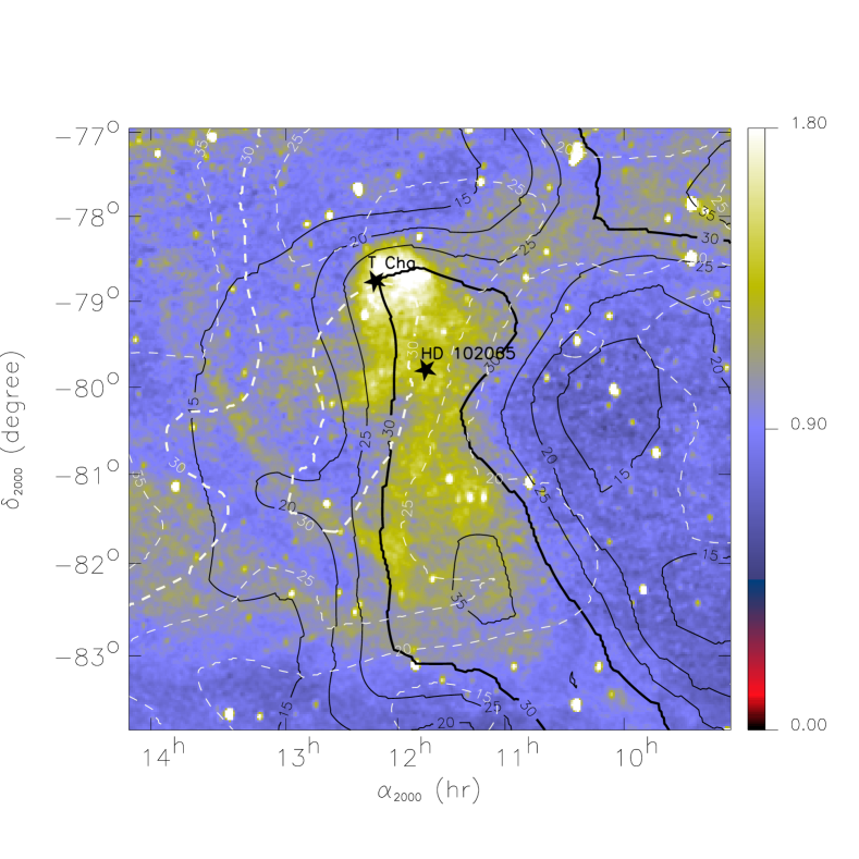
Figure 6: IRAS $12\mu m$ image (IRIS processing, Miville-Deschênes and Lagache, 2005) with contours of H i emission at $\rm V_{LSR}=-1{\rm\,km\,{s}^{-1}}$ (white dashed) and $5{\rm\,km\,{s}^{-1}}$ (black solid) taken from the IAR survey (30’ resolution and $1.3{\rm\,km\,{s}^{-1}}$ width velocity channels, Bajaja et al. 2005). The position of HD 102065 and the T Tauri star T Cha are marked. Contours are labeled with the brightness temperature. The 30 K contour is thicker. The cloud tail is roughly at a constant Galactic longitude. The Galactic coordinates of HD 102065 are $l\,=\,300.0^{\circ}$ and $b\,=\,-18.0^{\circ}$. The electronic version is in color.

In Figure 6, we show the spatial distribution of the H i emission in two-channel maps ($\rm V_{LSR}\,=\,-1$ and $+5{\rm\,km\,{s}^{-1}}$) overlaid over the IRAS 12$\mu$m image (Miville-Deschênes and Lagache, 2005), and in Figure 7 a position-velocity diagram across the Blue cloud at the Galactic latitude of HD 102065.

Figure 7: H i position-velocity diagram across the Blue Cloud at the Galactic latitude of HD 102065 (b=-18^∘). This figure shows that the two velocity components at respectively 0.1 and $4.2{\rm\,km\,{s}^{-1}}$ each extends on one side of the star position (l=300^∘) where they overlap. The emission at the OFF position (see text) has been subtracted to highlight the gas associated with the cloud.

These two figures show that the Blue Cloud, the bright IRAS 12$\,\mu$m emission on the map, is associated with gas at low velocities. The total brightness spectrum (thin line in Figure 5) shows the presence of a broad, negative velocity component, extending down to $-40{\rm\,km\,{s}^{-1}}$. This gas is not spatially correlated with the infrared emission from the Blue Cloud. It is however observed in UV-absorption spectra, and must therefore be located in front of the star.

species	$\rm V_{LSR}\,\,({\rm{km\,s}^{-1}})$	$\rm T_{b}\,\,{\rm(K)}$	$\rm FWHM\,\,({\rm{km\,s}^{-1}})$	$\rm b\,\,({\rm{km\,s}^{-1}})$	$\rm N\,\,({\rm{cm}^{-2}})$
H i   21 cm (difference)	$14.5\pm 0.6$	$0.9\pm 0.15$	$7.3\pm 1.4$	$4.4\pm 0.8$	$1.3\pm 0.2\,10^{19}$
	$4.2\pm 0.1$	$20.4\pm 1.1$	$3.2\pm 0.2$	$1.9\pm 0.1$	$1.3\pm 0.07\,10^{20}$
	$0.1\pm 0.1$	$13.4\pm 0.7$	$4.3\pm 0.3$	$2.6\pm 0.2$	$1.1\pm 0.06\,10^{20}$
	$-17.5\pm 0.6$	$1.0\pm 0.07$	$16\pm 1.4$	$9.4\pm 0.8$	$3.0\pm 0.2\,10^{19}$
CO(1-0)	$2.8\pm 0.2$	$7.0\,10^{-2}$	$3.5\pm 0.3$	$2.1\pm 0.2$	$6.9\,10^{13}\leavevmode\nobreak\ (J\,=\,1)$
CO(2-1)	$2.75\pm 0.17$	$3.6\,10^{-2}$	$3.0\pm 0.3$	$1.8\pm 0.2$	$1.8\,10^{13}\leavevmode\nobreak\ (J\,=\,2)$
		$I\,({\rm erg\,s}^{-1}{\rm cm}^{-2}{\rm sr}^{-1})$			N(C II*)
${\rm C^{+}\,158\mu m}$	-	$2.8\,10^{-6}$	-	-	$1.2\,10^{15}$

Table 4: Results from emission line measurements. H i measurements are performed on the difference spectrum (see text and Figure 5). The H i component at $14.5{\rm\,km\,{s}^{-1}}$ is not detected in absorption and is probably due to background gas situated behind the star HD 102065.

3.3 CO emission spectra

Long integrations have been performed with the 15m SEST telescope on the ¹²CO $J$=2-1 and $J$=1-0 emission lines.
The $J=$1-0 and 2-1 lines were observed in 1990 and 2001, with system temperatures of 700 K and 200 K respectively, and a velocity resolution of $0.1{\rm\,km\,{s}^{-1}}$. The rms noise level of the ¹²CO $J=$2-1 line displayed in Figure 1 is sufficiently low ($\sim 10$ mK) to reveal a broad and weak component ($\Delta v\,=\,2.9{\rm\,km\,{s}^{-1}}$, $T_{A}^{*}\,=\,36\,mK$), and a marginally-detected narrower component ($\Delta v\,=\,0.5{\rm\,km\,{s}^{-1}}$, $T_{A}^{*}\,=\,15\,mK$). The antenna temperature has not been corrected for beam coupling to the sky, because the source is much more extended than the telescope-beam size at this frequency ($\sim 22"$ or 0.015 pc at the distance of the cloud). This is not a critical issue because the beam efficiency was $\sim 0.85$ at 230 GHz. Similarly, the rms noise level of the $J=$1-0 line is $\rm 18\,mK$ for a velocity resolution of $0.2{\rm\,km\,{s}^{-1}}$. Given the weakness of the ¹²CO lines, the assumption of optical thinness is justified and the column densities of molecules in the $J=2$ and 1 levels are inferred from the line integrated intensities $W(CO)\,=\,0.1$ and $0.008\,K{\rm\,km\,{s}^{-1}}$ of the broad and narrow components of the $J=2-1$ line, and $W(CO)\,=\,0.2\,K{\rm\,km\,{s}^{-1}}$ for the J=1-0 line. The respective column densities are given in Table 4.

3.4 C⁺ observations

The ${\rm{C^{+}}}$ fine-structure transition at ${\rm{158\,\mu m}}$ has been measured towards HD 102065 with the Long Wavelength Spectrometer (LWS) of the Infrared Space Observatory (ISO), with a spectral resolution of $\rm R\,=\,300$, much lower than all other data presented in this paper. The data have been processed following the LWS handbook (Gry et al 2003). The resulting line intensity I(C⁺ $\lambda 158\mu$m) is $\rm 2.8\pm 1.0\,10^{-6}\,{erg\,s^{-1}\,cm^{-2}\,sr^{-1}}$, from which we estimate the C ii* column density N(C ii*)$\,=\,1.2\pm 0.4\,10^{15}\,cm^{-2}$. This is a measurement of the mean column density over the 80” LWS beam.

4 Analysis of the line of sight - Description of the interstellar components

4.1 The tool: Multi-lines fitting

To derive the characteristics of the interstellar components, i.e. column density $N$, velocity $v$ and broadening parameter $b$, we fit the observed line-profiles with theoretical ones, which are the results of the convolution of a Voigt profile with the instrumental function (LSF). We use a profile-fitting method, instead of a traditional measurement of equivalent width, because the velocity structure is complex as can be seen in Figures  1 to 3. Because several components are blended together in most lines, profile fitting is required to derive the characteristics of the individual components. The data fitting has been performed with the use of the profile fitting software “Owens.f” developed by Martin Lemoine.

The software allows several lines of the same element, as well as lines from different elements, to be fitted together. It also allows several velocity components to be fitted simultaneously, and the components to be included in the absorption profiles for each element to be specified. The software therefore derives a global and consistent solution for a group of species. Multiple iterations are necessary to find which species could be fitted in a consistent way with the same velocity components. A common component for different species obviously implies a common absorption velocity but also common physical conditions, implying consistent broadening parameters.

The fitting software breaks the line-broadening parameter (b-value) into thermal broadening, which depends on the element mass, and non-thermal broadening (turbulence), which is the same for all elements in a component. Therefore, fitting lines from elements of different masses simultaneously, in principle enables the simultaneous measurement of temperature, turbulent velocity, the velocity itself, and column densities. In practice interstellar absorption lines are usually found to be of two types. The first type displays unsaturated lines from heavy elements that have similar b-values independently of the element mass: in this case, the broadening is primarily non-thermal, implying that T is low and can be estimated only if the analysis includes an element whose mass is low enough to introduce a significantly different b-value. Here we will consider H i emission lines. In the case of the second type of interstellar absorption line, the b-values vary with element mass due to a significant thermal effect, implying that T is high and can be estimated. In practice the interstellar absorption lines are broader than the resolution element (for T higher than a few thousand K), and strong lines are occasionally broadened considerably by saturation, leading to the blending of components and limiting the precision with which broadening parameters can be derived.

The quality of the fits, and the error bars on column densities, have been computed using the $\Delta\chi^{2}$ method described, for example, in Hébrard et al (2002). We performed several fits by fixing the column density of a given element ${\rm X}$ to a different value in each fit. In all of these fits, all other parameters are not fixed and we compute the best $\chi^{2}$ for each value of column density. The plot of $\Delta\chi^{2}$ versus $N(X)$ provides the 1, 2, 3, 4, $5\,\sigma$ range for $N({\rm X})$. This is illustrated with an example in Figure 8.

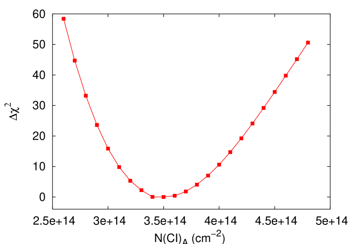
Figure 8: Example of a $\Delta\chi^{2}$ curve, here for C i in component A. Each point corresponds to a fit performed with the C i column density in component A fixed to the value given in abscissa. $\Delta\chi^{2}$ is rescaled by dividing it by the 95 %-confidence level for this fit (rescaled $\Delta\chi^{2}=1.41$). 3$\sigma$-uncertainty is given by $\Delta\chi^{2}=3^{2}\times 1.41=12.7$.

Examples of the fits are presented in Figure 1 for molecules, Figure 2 for neutrals, and Figure 3 for ions.

4.2 Component structure and velocities

4.2.1 Atoms with ionization potential lower than H i.

The common asymmetry of the absorption lines of the neutral species (Figure 2) suggests the existence of two velocity components in all of these lines. When fitting simultaneously C i, C i*, C i**, S i and Fe i, a best fit is achieved for two components, that we call component A and component B, for the following LSR velocities: $\rm V_{LSR}=3.8$ and $0.4{\rm\,km\,{s}^{-1}}$. They may be converted into heliocentric velocities by adding $10.2{\rm\,km\,{s}^{-1}}$.

The b-values derived in the fits, $b_{{\rm A}}=1.5\pm 0.2$ and $b_{{\rm B}}=1.6\pm 0.2{\rm\,km\,{s}^{-1}}$ are not significantly different for the three species with different masses. This is strong support to the fact that broadening is primarily non-thermal.

Interestingly, the velocities identified for the two main components in the H i Blue Cloud emission spectrum (see Table 4) are identical to those of A and B within the error bars. The b-values are also similar to those expected in cool gas, with the H i b-values being slightly higher than that of S i and C i due to the mass difference. The main components seen in emission are therefore likely to be related to the two main components observed in absorption.

4.2.2 Molecules

In contrast, the CO lines do not accept a two-component solution. The singularity of the CO component is evidenced by the small width of the CO lines, with $b_{CO}=1.6\pm 0.2\,{\rm km\,s^{-1}}$, similar to that of component A or B alone. This width is significantly lower than the velocity difference between A and B, $3.3\,{\rm{km\,s}}^{-1}$, toward which value $b_{CO}$ would tend to increase if CO was distributed over the two components. When fitting the ${\rm{CO}}$ lines in a two-component model together with all well-behaved (i.e. not heavily saturated) neutral lines, unavoidably in the resulting fit most of the ${\rm{CO}}$ column density is found in one of the components, and the resulting theoretical profile appears slightly shifted relative to the observations. This component cannot be identified with either A or B, since its velocity shift is significantly higher than the uncertainty of the wavelength calibration in a single STIS sub-spectrum. Alternatively, when fitting the neutrals and ${\rm{CO}}$ lines altogether in a one-component model, the fit to the neutral lines is significantly degraded. The line characteristics (central velocity and line width) of CO in emission agree with that derived from UV absorption lines. This agreement validates the UV wavelength calibration and confirms that CO, unlike H i and the atomic species C i and S i, is found at a single velocity.

We infer that ${\rm{CO}}$ is detected primarily in one component at a velocity intermediate to that of A and B, $\rm V_{LSR}{\rm CO}=2.7\,{\rm{km\,s}^{-1}}$. We will call this component C (see Figure 1 illustrating the line fit for two CO bands).

Further information is provided by the CH and CH⁺ absorption line profiles. We performed the profile fitting of the CH and CH⁺ lines with Owens together with the STIS data of the species C i, S i and CO. We made several fits with CH and CH⁺ either using one or two components, and with a velocity shift as a free parameter to take into account uncertainties in the absolute wavelength calibration of both the UV and optical spectra. The best results have been obtained if (i) CH⁺ is present in both components A and B and (ii) most of the CH absorption is in one component, corresponding to the CO component C. This solution implies that the optical spectra are shifted by about 0.3 ${\rm\,km\,{s}^{-1}}$ relative to the STIS data, a value consistent with the wavelength calibration uncertainty.

We conclude that the bulk of the CO and CH molecules are in a single component (C) at a different velocity to the bulk of the neutral atoms carbon, sulfur, iron and hydrogen and the CH⁺ molecules, which appear to be distributed over two well-separated velocity components (A and B). Of course it is not excluded that some neutrals are present at the velocity of CO, and alternatively that some CO is present in the components A and B, at undetectable levels. We believe that the three components A, B and C are, in fact, physically related. Within this assumption, the three velocity components would reflect the particular velocity structure associated with local abundance variations within a single cloud.

4.2.3 Ions and neutrals with ionization potential higher than H i.

Almost all ions and neutrals with an ionization potential slightly higher than H i: Mg ii, Mg i, Mn ii, P ii, Ni ii, C ii, N i and O i, can be fitted altogether with a unique solution for the line of sight structure : component 1 at $2.5\pm 0.3\,{\rm{km\,s}^{-1}}$, component 2 at $-5.5\pm 0.2\,{\rm{km\,s}^{-1}}$, component 3 at $-11.0\pm 0.2\,{\rm{km\,s}^{-1}}$ and component 4 at $-18.7\pm 0.2\,{\rm{km\,s}^{-1}}$ (velocities are LSR, see Table 5).

The low-velocity component, component 1, corresponds to the gas detected in neutral and molecular lines. In the unsaturated ion lines this component can be fitted either with two components at the velocity of A and B, or with a single component at the intermediate velocity $\rm V_{LSR}\,=\,2.5\,\pm\,0.3\,{\rm{km\,s}^{-1}}$ without affecting the column density results or the quality of the fits (monitored by the $\chi^{2}$). However when adding stronger lines to the fit, it has been impossible to find a good fit to the spectra in component 1 with the column density provided by the unsaturated lines and the A+B velocity structure. This suggests that the structure of this component is more complex and may indicate the presence of warmer gas at the velocity of component 1. Even with a low column density, in strong lines warm gas can contribute a large part of the equivalent width due to a larger b-value. For the ions, we therefore quote a unique column density, obtained using the unsaturated lines when they exist, for the low velocity component 1 alone.
The components structure is summarized in Table 5.

4.3 Column densities

4.3.1 Column densities from absorption lines

Once the velocity structure is defined, column densities can be derived following the method described in section 4.1. In this respect, not all of the lines are equally useful.

Fe ii is the most favorable ion in our sample for two reasons. First, several Fe ii lines are available with a large range of f-values from 0.0014 to 0.32 (see Table 2). Strong lines allow detection of weak components, and weak lines enable non-saturated profiles of strong components to be analyzed. Another advantage of Fe ii lines is that, due to its high mass, Fe is less affected by thermal broadening than lighter elements; therefore in warm gas Fe ii absorption lines are narrower and the components better-resolved as seen on Figure 3. The errors in N(Fe ii) are therefore due only to the combination of noise and uncertainty in the continuum placement.

We achieve our poorest quality analyses for ions for which only strong lines are available. This is the case here for C ii, C ii^∗ and Si ii, for which all components are saturated and for which we can derive only lower limits.

When only one weak line for a given element is detected, only the strongest component 1 is detected and measured and we get column-density upper limits for all other components. This is the case for both Ni ii and P ii.

For some elements, we have both a very weak line, which is only detected in the strongest component, allowing measurement of the column density, and very strong lines that are saturated in all components. Combining weak and strong lines gives upper and lower limits for the weak components. This is the case for Mg ii $\lambda 1240\textrm{\AA}$ and O i $\lambda 1356\textrm{\AA}$, which are respectively $4.4\times 10^{4}$ and $10^{3}$ times weaker than the strong lines Mg ii $\lambda 2800\textrm{\AA}$ and O i $\lambda 1302\textrm{\AA}$. S ii is an intermediate case where the three S ii lines are saturated in component 1 and at least one S ii line is unsaturated in the other weaker components. The uncertainty in their column density is due to blending between components and uncertainty in the continuum placement.

As mentioned in Section 2.2, Si ii* and O i** are detected primarily at the velocity of component 4, while they are hardly detectable in components 1, 2 and 3. Nevertheless O i* is detected in the four components.

Column densities resulting from absorption line fitting are provided in Table 5.

Component	A	C	B
$\rm V_{LSR}\,({\rm{km\,s^{-1}}})$	3.8$\pm 0.1$	2.7$\pm 0.2$	0.4$\pm 0.1$
T (K)	$85\pm 65$	-	$270\pm 100$
$\rm b_{NT}\leavevmode\nobreak\ ({\rm\,km\,{s}^{-1}})$	1.5$\pm 0.2$	1.6$\pm 0.2$	1.5$\pm 0.2$
${\rm{CO}}\,J=0$		$3.3\pm_{0.5}^{0.3}\,(13)$
${\rm{CO}}\,J=1$		$2.1\pm_{0.3}^{0.4}\,(13)$
${\rm{CO}}\,J=2$		$<2.5\,(12)$
${\rm CH}$		$6.5\pm 1.5\,(12)$
${\rm CH^{+}}$	$9\pm 2\,(12)$		$4\pm 1\,(12)$
C i (${}^{3}P_{0}$)	$3.5\pm_{0.3}^{0.5}\,(14)$		$1.3\pm_{0.3}^{0.2}\,(14)$
C i* (${}^{3}P_{1}$)	$6.6\pm_{0.7}^{0.8}\,(13)$		$2.7\pm 0.5\,(13)$
C i**(${}^{3}P_{2}$)	$1.1\pm 0.15\,(13)$		$3.0\pm_{1.1}^{2.2}\,(12)$
S i	$4.4\pm_{0.5}^{0.6}\,(12)$		$2.0\pm 0.5\,(12)$
Fe i	$1.50\pm 1.0\,(11)$		$<2.81\,(10)$
Component	1 (A+B)			2	3	4
$\rm V_{{\rm LSR}}\,({\rm{km\,s^{-1}}})$	$2.5\pm 0.3$			$-5.5\pm 0.2$	$-11.0\pm 0.2$	$-18.7\pm 0.2$
T (K)	-			8 500 $\pm 1\,500$	13 000$\pm 3\,000$	$\sim 20\,000-\geq 200\,000$
Fe ii	$2.2\pm\,1.1\,(14)$			$1.2\pm_{0.3}^{0.1}\,(13)$	$1.3\pm 0.2\,(13)$	$1.4\pm 0.2\,(13)$
Mg ii	$1.8\pm_{0.5}^{0.3}\,(15)$			$1.9\,(12)\mapsto 1.2\,(14)$	$2.3\,(12)\mapsto 1.5\,(14)$	$2.9\,(12)\mapsto 1.6\,(14)$
S ii	$>3.0\,(16)$			$5.0\pm_{1.5}^{2.0}\,(13)$	$1.0\pm 0.2\,(13)$	$1.1\pm_{0.2}^{0.4}\,(14)$
P ii	$2.5\pm 1.0\,(14)$			$<1.6\,(13)$	$<2.4\,(13)$	$<2.7\,(13)$
Mn ii	$1.3\pm_{0.1}^{0.2}\,(13)$			$1.2\pm 1.0\,(11)$	$1.6\pm 1.0\,(11)$	$1.4\pm 1.0\,(11)$
C ii	$>1.3\,(14)$
C ii*	$>1.3\,(14)$
Si ii	$>1.0\,(14)$
Si ii*	$<2.4\,(12)$			$<1.6\,(12)$	$<1.8\,(12)$	$>3.2\,(13)$
Ni ii	$7.0\pm 2\,(12)$			$<1.6\,(13)$	$<1.2\,(13)$	$<1.4\,(13)$
Mg i	$2.25\pm_{0.28}^{0.5}\,(12)$			$<2.1\,(11)$	$<2.1\,(11)$	$7\pm 4$$\,(10)$
O i	$4.1\pm 1.6\,(17)$			$3.2\,(13)\mapsto 6.2\,(16)$	$3.4\,(13)\mapsto 4\,(16)$	$3.1\,(13)\mapsto 3.7\,(16)$
N i	$2.0\pm 1.0\,(17)$			$1.5\,(14)\mapsto 1.2\,(16)$	$2.7\,(14)\mapsto 1.9\,(16)$	$3.0\,(14)\mapsto 1.2\,(17)$
S iii						$<2.4\,(13)$
Si iii						$>6\,(12)$
Si iv						$8.2\pm 3.2\,(12)$
C iv						$1.45\pm 0.6\,(13)$

Table 5: Interstellar component characteristics derived from the absorption lines in the UV and optical spectrum. The ions absorption in component 1 may be distributed over the velocities of components A and B however the fits have been performed with one component. Velocities: The listed uncertainties on $V_{LSR}$ apply to relative velocities. The absolute uncertainty from the precision of the STIS wavelength calibration is about $1.2\,{\rm{km\,s}}^{-1}$, absolute velocities have however been confirmed to about $0.3\,{\rm{km\,s}}^{-1}$ by the good agreement between component C and the CO emission in the heterodyne data, which have an absolute precision of $0.1\,{\rm{km\,s}}^{-1}$. Temperature: When possible, temperatures are derived from the combination of $b$-values from species of different masses. The precise temperatures for components A and B have been derived under the assumption that they can be identified to the two components seen in emission in the Blue Cloud H i spectrum. Column densities (in cm^-2): Numbers in parentheses are powers of 10. All error bars are 3 $\sigma$ uncertainties, except for the intervals given by the arrows, indicating and upper limit derived from a faint line and a lower limit derived from a strong saturated line. Si ii, C ii and C ii* profiles are saturated for all components, implying that only a lower limit could be derived for the whole absorption.

4.3.2 Comparison of absorption/emission column densities

In this section, we compare column densities derived from emission and absorption spectra.

The total hydrogen column density can be estimated from the color excess, and the standard ratio $N({\rm H}_{tot})/E({\rm{B-V}})=5.8\times 10^{21}\,{\rm{cm}}^{-2}\,{\rm{mag}}^{-1}$ (Bohlin et al., 1978). This provides a measurement of $N({\rm H}_{tot})=9.8\times 10^{20}$ cm^-2. It can also be derived in addition using H₂ column densities measured in FUSE absorption spectra (Table 1), and the H i column density estimated from the Blue Cloud H i emission spectrum : $N({\rm H}_{tot})=N({\rm H})+2N({\rm H_{2}})=9.6\times 10^{20}\,{\rm cm}^{-2}$ excluding the $14.5{\rm\,km\,{s}^{-1}}$ background component (Table 4). The quantitative agreement between emission and absorption results for column densities, velocities, and line widths, supports the idea that the two H i low velocity components observed in the Blue Cloud H i emission spectrum correspond to components A and B observed in absorption.

One can also note that there is a consistency between the C⁺ column density derived using ISO-LWSdata, and the lower limits measured from the saturated absorption lines.

CO column densities were measured both in emission and absorption. In absorption, they can be directly compared to the H₂ column densities derived from FUSE spectra (Gry et al., 2002). This comparison enables the measurement of a total CO abundance $N({\rm CO})/N({\rm H_{2}})\,=\,1.5^{+0.2}_{-0.15}10^{-7}$.

It was interesting to find that the CO column densities were larger when determined in emission than in absorption, by a factor 3 in the $J\,=\,1$, and by more than a factor of 7 for the $J\,=\,2$ level. Because the spatial resolutions of the observations are very different, this could imply the existence of small-scale structure of the CO emitting gas within the SEST beam. On the other hand, part of the CO emission could be background emission from the envelope of the nearby Chamaeleon III cloud, which is observed over the same velocity range (Mizuno et al., 2001). Based on measurement of the CO excitation, we consider that this second possibility is however unlikely. The column density ratio between the $J=2$ and 1 levels, derived from the emission spectrum provides an excitation temperature $T_{ex}\,=\,2.9\,$K (population ratio $N(J=2)/N(J=1)=0.24$), a value very close to the Cosmic Microwave Background temperature. The low excitation implies that collision excitation of the CO transitions by H or H₂, is negligible when compared to radiative excitation, hence the local density is much lower than the critical density of the 2-1 transition $n_{H}=10^{4}\,$cm^-3. However, if the gas was associated with the Cham III cloud, we expect that radiative excitation alone could produce a higher $T_{ex}$.

4.4 Temperatures

As noted in Section 4.1, information on the temperature of the gas in each component follows from the ability to fit simultaneously lines from several elements of different masses, which allows the nature of the broadening to be determined.

4.4.1 Cool gas

For components A and B, the similarity of the $b$-values for lines from heavy elements of different atomic masses (see Section 4.2) suggests that their widths are dominated by non-thermal motions. To estimate the gas temperature, we compared heavy-element line-widths to the widths of the associated H i line emission.

Although the beam of the H i emission observations is several orders of magnitude larger than the pencil beam of UV absorption observations ($0.5^{\circ}$ vs milli-arcseconds), we assume that the samplings of the velocity field are similar. By computing spectra produced by numerical simulations of mildly compressible turbulence, Pety and Falgarone (2000) showed that one-dimensional sampling of a turbulent, homogeneous field is similar to that performed by an extended beam. This behavior of the linewidths is indeed found in mm-line observations of CO in emission and absorption against extragalactic sources (Liszt and Lucas, 1998). Once the H i linewidths are included in the analysis, the temperatures, yielded formally by the $b$-value differences between H i and heavy neutrals, are 85 $\pm 65$ K for A and 270 $\pm 100$ K for B. For both components, the non-thermal velocity contribution to the linewidths is $\sim 1.5$ km s^-1. We note that these temperatures apply to the atomic species, and not necessarily to CO and CH because these molecules appear to be kinematically-decoupled from the atomic species.

4.4.2 Warm gas

Components 2 to 4 belong to the second type of interstellar absorption lines, and T is estimated using the UV-line fitting procedure. Component 2 has a temperature typical of warm diffuse gas ($7\,000$–$10\,000\,{\rm K}$), while in Component 3 and 4 the thermal broadening is clearly dominant, with temperatures of $13\,000\pm 3\,000\,{\rm K}$ for component 3, and about $20\,000\,{\rm K}$ for component 4 as derived from weak and moderate lines. In the latter, a more precise determination of T is impossible because gas of different temperatures appear to be present at this velocity.

4.4.3 Hot gas

Indeed the strong Mg ii lines show the presence of additional high temperature gas at approximately $200\,000\,{\rm K}$, moving at a velocity close to that of component 4. The presence of high temperatures is well-illustrated by the clear difference between the blue wings of the Mg ii profile and the N i profile in Figure 3. While the relatively steep blue wing of the N i line can be fitted with a temperature close to $20\,000\,{\rm K}$ for component 4, the extended blue wing in Mg ii requires the addition of a hot component at the same velocity, of a temperature $\sim 200\,000\,{\rm K}$, and a column density about 10% of that of the total column density of component 4. If this extended blue wing was a damping wing due to a component with very high column density, this component would create a significative absorption in the faint Mg ii line at 1240 Å, at least as strong as that of component 1. However, no additional component is detected significantly in Mg ii $\lambda$1240Å. The blue wing can therefore only be due to high-temperature, low-column density gas.

High temperatures are also detected for the excited species. The presence of hot gas is traced by the large width of the Si ii* lines compared to the width of other lines of moderate strength. The FWHM of the Si ii* line, shown in Figure 3, is $\sim 18$ ${\rm{km\,s}^{-1}}$, corresponding to $\sim 200\,000\,{\rm K}$. In the C ii* line, the blue wing is extended, up to LSR velocities of $-50\,{\rm{km\,s}^{-1}}$. This may correspond to the presence of very high temperature gas at a velocity close to that of component 4, as in the case of Mg ii.

The high-ionization species Si iii, Si iv and C iv have been detected in the spectra at the velocity of component 4. They are broad and the temperature implied by their width is at least $200\,000\,$ K. A temperature close to $10^{6}$ K, is in fact consistent with the observations (see figure 4 for an illustration), although the large width of the lines could be due to the presence of several components at a temperature of a few $10^{5}$ K. OVI is unfortunately not available in absorption in the FUSE spectra, because the stellar continuum is too weak at these wavelengths.

4.5 Summary of the line of sight

The description of the line of sight that emerges from the direct analysis of the spectral data is complex. The bulk of the gas is at low LSR velocity. Neutral low-potential atoms and most of the H i are distributed over two components separated by $\sim 3{\rm\,km\,{s}^{-1}}$(called A and B) that appear in these species to have temperatures of at most a few hundred K, and are associated with CH⁺. The molecules CO and CH however, are within a single component of similar b-value ($b\sim 1.5{\rm\,km\,{s}^{-1}}$) at a velocity intermediate between that of A and B.

Other components exist at high negative velocities with respect to the bulk of the gas. Negative-velocity gas is seen in the absorption lines of ions and atoms with ionization potentials higher than that of H i, as well as in emission in H i. The temperature of these components ranges from typical temperatures of diffuse atomic gas ($\sim 10\,000\,$K) to somewhat higher temperatures (comparable to $20\,000\,$K), and increases with velocity offset from the bulk of the gas, in addition to the gas excitation state. The highest velocity component, while evident for moderately-ionized species, of temperature approximately $20\,000\,$K, is associated with highly-excited, highly-ionized hot gas of temperatures up to several $10^{5}$K.

5 The cool gas and its traces of warm gas

The bulk of the gas detected along the line of sight, is cool diffuse molecular gas at low velocities. We comment on its properties within the framework of diffuse clouds studies.

Diffuse molecular clouds are often modeled as extended, homogeneous, low-density structures with properties regulated by the progressive extinction of the UV field by dust. In a companion paper (Nehmé et al. 2007), we show that most observations of the cold, low-velocity gas, namely the H₂ abundance and ortho-to-para ratio, the CO abundance, the C i abundance and excitation, and the 158$\mu$m C ii line emission fit with model computations for a diffuse molecular cloud of a gas density of $80\,$cm^-3, illuminated by a UV radiation field close to the mean Solar Neighborhood value. The gas temperature, derived from the balance between cooling and heating processes, ranges from 60 to 80 K. Combining the gas density and gas temperature we calculate a thermal pressure, $P/k\sim 5000{\rm cm}^{-3}{\rm K}$, which is within the range of values measured by Jenkins (2002), for clouds within the local Bubble. While the physical conditions inferred from the model probably apply correctly to the bulk of the gas, we hereafter discuss two points that show the limitations of the model’s simplicity.

The first point is the apparent kinematic separation of molecular and atomic species in the cool gas, with the distribution of atomic species and CH⁺ over two velocity components A and B, and the molecules CO and CH observed at a single intermediate value of velocity. As noted in Section 4.2, we believe that these components are related and therefore treat them as a single cloud in the modeling. However, the observed velocity structure of the cloud cannot be accounted for by the photon-induced chemistry model where most of the C i, CO and H₂ are predicted to occupy the same volume (see figures 3 and 4 in Nehmé et al. 2007).

The second point is the existence of traces of warm molecular gas, as indicated by a CH⁺ absorption line, and a population of $\rm J>2$ H₂ rotational levels that exceed model values by almost two orders of magnitude. Falgarone et al. (2005) determined an average Galactic-fraction of warm H₂, in cool diffuse gas, expressed as the ratio of the column density of H₂ molecules in levels $J>2$ (or $N({\rm H}_{2}^{*})$ per magnitude of gas sampled: $N({\rm H}_{2}^{*})/A_{V}=4\times 10^{17}\,$ cm^-2. The warm H₂ predicted along the line of sight to HD 102065, with this average Galactic fraction, would then equal $N({\rm H}_{2}^{*})=2.7\times 10^{17}\,$cm^-2, compared to the range 1-3 $\times 10^{17}\,$cm^-2 given in Table 1. The ratio of the CH⁺ to the total hydrogen column densities towards HD 102065 $N({\rm CH^{+}})/N_{H}=1.2\times 10^{-7}$, is comparable to the values calculated in previous observations by Crane, Lambert & Scheffer (1995) and Gredel (1997). The formation of CH⁺ in diffuse gas involves the endothermic reaction C⁺ + H${}_{2}\rightarrow$ CH⁺ + H ($\Delta E/k=4640$ K), and has to be triggered by deposition of supra-thermal energy either in MHD shocks (Flower & Pineau des Forêts 1998), or in large velocity shears (Joulain et al. 1998).

The chemical patterns triggered by the local deposition of non-thermal energy involve several other endothermic reactions, including CH destruction, which produces neutral carbon. According to the models explored in Joulain et al. (1998), the column density of C i produced in the warm chemistry $N({\rm C_{w}})$, scales with that of CH⁺ as $N({\rm C}_{w})\approx 3N({\rm CH^{+}})$ or $N({\rm C}_{w})\approx 3\times 10^{13}$ cm^-2. This corresponds to less than 10% of the total C i column density $N({\rm C})=5.7\times 10^{14}$ cm^-2 detected in components A and B (see Table 5). The domain of parameters influencing the out-of-equilibrium chemistry is difficult to explore, and this is only an estimate provided by existing models. The production of CO is enhanced by the warm chemistry patterns, due to enhanced production in the warm gas of OH, HCO⁺ and CH${}_{3}^{+}$, all chemical precursors of CO. It is possible that the observed heterogeneity of CO abundances discussed above, originates in such processes.

6 HD 102065 gas components within the local bubble context

In this section, we place the HD 102065 observations in a broader context by relating them to the interaction between the nearby interstellar medium, and the Sco-Cen OB association, the Local and the Loop I Bubbles.

Based on an extensive study of colour excess versus distance for a large sample of stars within $\rm 294^{\circ}<l<308^{\circ}$ and $-20^{\circ}<b<5^{\circ}$, Corradi et al. (1997) concluded that the local density of matter is low until an extended interstellar dust feature at $150\pm 30\,$pc from the Sun associated with the Chamaeleon, Musca and Southern Coalsack dark clouds. The same authors complemented their investigation with NaI absorption spectra. Absorption lines at negative velocities are detected towards many stars including the stars closest to the Sun (Corradi et al. 2004), which is indicative of a low column density ($\rm N_{H}\sim$ a few $\rm 10^{19}\,cm^{-2}$), nearby ($d<60\,$pc) sheet of gas, outflowing from the Scorpius-Centaurus stars with mean radial velocity $\rm V_{LSR}=-7{\rm\,km\,{s}^{-1}}$. The presence of such a sheet was first proposed by Egger and Aschenbach (1995) to account for the soft X-ray shadow seen in the ROSAT All Sky Survey maps.

In the northern sky, the Loop I shell extends up to North Polar radio spur. In the southern sky, a broad H i filament at $b=-35^{\circ}$ and $\rm V_{LSR}\sim-20{\rm\,km\,{s}^{-1}}$ marks the outer extension of gas swept up by the 10-15 Myr old LCC and UCL subgroups (de Geus 1992).

In the Argentine H i survey (Kalberla et al. 2005 and Bajaja et al. 2005), H i gas at velocities $\rm V_{LSR}<-20{\rm\,km\,{s}^{-1}}$, down to $-50{\rm\,km\,{s}^{-1}}$, is visible over $60^{\circ}$ in longitude about the Sco-Cen sub-groups (see Figure 9). The selection in radial velocity focusses on gas streaming towards the Sun at the center of Loop I. We note also that much of the negative velocity gas close to the Upper-Scorpius (US) group that still contains O stars must be photo-ionized and thus not seen in H i. The H i survey data show that negative velocity gas is clumped and scattered over a wide range of negative velocities, which cannot be accounted for within the simple picture of an expanding shell about a localized group of massive stars. We propose instead that we are looking at dispersed fragments of the parent cloud of the LCC and UCL stars accelerated to a range of velocities by supernovae blast waves. Since the stellar groups have moved with respect to the Sun (de Zeeuw et al. 1999), the explosions have occured at different locations and distances from the Sun fragmenting and spreading the stars’ parent cloud between the Local and Loop I bubbles. This view accounts for the stream of negative-velocity gas observed close to the Sun, including the local cloud about the Sun, detected at negative velocities, streaming from the general direction of the Sco-Cen association (Ferlet 1999). Our view of the relation between the nearby interstellar medium and the Sco-Cen stars, the Local and Loop I bubbles builds on the original scenario proposed by Breitschwerdt et al. (2000). However, the observations suggest a more complex picture where there is not a continuous sheet of swept-up gas separating the two bubbles, but instead clouds of cold and warm gas spread out between the two bubbles.

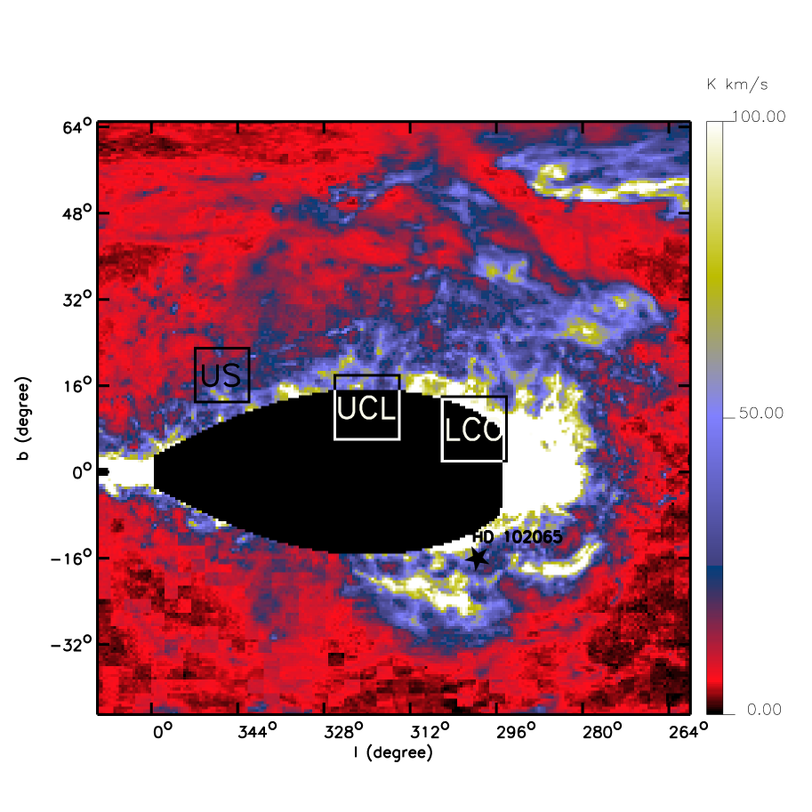
Figure 9: H i emission at negative velocities $\rm-50<V_{LSR}<-20{\rm\,km\,{s}^{-1}}$ in direction of the Sco-Cen association. H i observations from Bajaja et al. (2005) and Kalberla et al. (2005). The position of HD 102065 and the US (Upper-Scorpius), UCL (Upper Centaurus Lupus) and LCC (Lower Centaurus Crux) sub-groups of the OB association are marked. The black area indicates the region where the selected range of negative velocities overlaps with the Galactic rotational velocities of distant gas. The electronic version is in color.

We believe that the diffuse molecular cloud in the foreground of HD 102065, is such a cloud. As discussed by Mizuno et al. (2001), there is strong evidence that Dcld 300.2-16.9 (the Blue Cloud) is not part of the Chamaeleon molecular clouds complex. A distance of $70\pm 15\,$pc from the Sun, is inferred from the parallax of the T-Tauri star T Cha, which coincides in position and velocity (Covino et al. 1997) with the cloud CO emission. This places the cloud at a distance of $\sim 30$ pc from the center of the LCC sub-group (de Geus 1992). Its cometary structure, with a tail extending in the opposite direction to that of the LCC stars, suggests that it could have been shaped by a supernova explosion from one of the stars. With a total mass of $\rm\sim 100\,{\rm M_{\odot}}$ (including the tail, as calculated by Boulanger et al. (1998) and corrected assuming a distance of $70\,$pc), the cloud is too massive to have been globally accelerated by a distant explosion but its structure suggests that gas ablated from the surface by the blast wave is streaming outwards. In the H i data, the low velocity components A and B are connected to the cloud head but extend in different directions along the cloud tail (Figure 6). This may imply that they represent both sides of the gas flow, that they encompass the cloud core, and that the difference in radial velocity is the result of a difference in angle between the streaming direction, and the line of sight. At the surface of the gas flow, the CO and CH molecules are photodissociated, explaining why they are not detected in components A and B, but instead in a single component C, which would correspond to the internal part of the gas flow. To account for the $3{\rm\,km\,{s}^{-1}}$ velocity difference between components A and B within a reasonable angle difference ($\sim 45^{\circ}$), the gas streaming velocity must be $\sim 10{\rm\,km\,{s}^{-1}}$. The tail length $\sim 2^{\circ}$ ($2.4\,$pc for a distance of $70\,$pc) translates into a time elapsed since the supernova explosion of $\sim 2-3\times 10^{5}\,$yr. The HD 102065 observations were originally motivated by the strong mid-IR emission of the foreground cloud interpreted as an unusually high abundance of small dust grains (Boulanger et al., 1990). This distinct characteristic may be related to the position of the cloud within the Local Bubble, and its plausible interaction with a supernova blast wave.

The interaction between interstellar clouds and shock waves travelling in their surrounding medium, has been investigated using numerical simulations. Images presented in Nakamura et al. (2006) help to picture the complexity of the interaction that ablates matter from the cloud and generates a turbulent flow streaming away from the cloud. The fact that the C iv and Si iv absorption lines peak at negative velocities qualitatively agrees with this picture where one expects the low density gas in the turbulent mixing layer to be entrained by the flow of hot gas. The discrepancy between gas temperature and ionization state evident for some of the Mg ii, Si ii^∗ and C ii^∗ observed at a temperature $2\times 10^{5}\,$K, implies that dynamical mixing of hot and warm gas, on timescales shorter than that necessary to reach ionization equilibrium, is taking place.

7 Conclusion

High resolution spectroscopic observations are presented and used to characterize the physical state and velocity structure of the multiphase interstellar medium observed towards the nearby star HD 102065. These spectroscopic observations provide detailed information on the kinematics and physical state of the gas, along the line of sight.

• Gas is observed over a wide range of velocities, with cold molecular gas at low velocities, and warmer and lower density gas at negative velocities. Most of the hydrogen column density is in cold diffuse molecular gas at low LSR velocities.

• The spectra show three distinct components at negative velocities as low as $\rm V_{LSR}=-20{\rm\,km\,{s}^{-1}}$. The excitation and temperature of the species detected in the negative velocity components, increase with the velocity separation from that of the diffuse cloud. H i emission maps show that the negative velocity gas extends over $\rm\sim 200\,{\rm deg}^{2}$. It is fragmented and spreads over velocities down to $-50{\rm\,km\,{s}^{-1}}$.

• A striking result of the data analysis is the detection of gas out of equilibrium in both the low and the negative velocity gas. At low velocities, we find that the cold molecular gas is mixed with traces of warmer molecular gas where the observed CH⁺ must be formed and which is also traced by the observed excess population of H₂ in the $J>2$ levels. At negative velocities, gas in a low ionization state (Mg ii, Si ii^∗ and C ii^∗) is observed far out of ionization equilibrium at a temperature of $2\times 10^{5}$K.

We have set the observational results within the scenario proposed by Maiz-Apellaniz (2001) and Berghöfer and Breitschwerdt (2002) that connects the origin of the Local Bubble to supernovae explosions from early star members of the oldest Sco-Cen groups.

• The gas at low LSR velocities is observed to be associated with the Blue Cloud (Dcld 300.2-16.9) located within the local bubble at a distance of $\sim 70$pc from the Sun. Its cometary shape with a tail pointing away from the LCC sub-group of the Sco-Cen association $\sim 30$pc away, strongly suggests that it has been shaped by the interaction with a recent ($2-3\times 10^{5}\,$yr) supernova explosion from one of the LCC stars. The line of sight to HD 102065 goes across the cloud tail. The velocity structure of the low velocity gas may be understood as the two sides of a flow of gas ablated from the cloud head Dcld 300.2-16.9. The large abundance of small dust particles inferred from the IRAS colors of the Blue Cloud tail, possibly results from the cloud interaction with the supernova blast wave.

• The negative velocity gas must have been accelerated by a supernova explosion that occurred in the Sco-Cen OB association. Our interpretation of the Blue Cloud shape would imply that it is physically connected with the lower velocity gas. The column density of Si ii^∗ at $-20{\rm\,km\,{s}^{-1}}$ might be a signature of an ongoing shock.

A complete diversity of diffuse interstellar-medium components, is present along the line of sight. Our analysis of both low and negative velocity, hot, warm and cold gas components, stresses the complex dynamical interplay between the interstellar medium phases, in agreement with the predictions of numerical simulations (Audit and Hennebelle 2005, de Avillez and Breitschwerdt 2005). We started this work by considering an apparently unusual cloud, but now believe that the questions we are now asking, have significance for the general study of diffuse, interstellar matter in the Galaxy.

- (1) Audit, E., Hennebelle, P. 2005, A&A 433, 1
- Bajaja et al. (2005) Bajaja, E., Arnal, E. M., Larrate, J. J.,Morras, R., Pöppel, W. G. L. and Kalberla, P. M. W. 2005, A&A 440, 767
- Beideck et al. (1994) Beideck, D. J., Schectman, R. M., Federman, S. R. & Ellis, D. G. 1994, ApJ, 428, 393
- (4) Berghöfer, T. W., Breitschwerdt, D. 2002, A&A 390, 299
- Bohlin et al. (1978) Bohlin, R. C., Savage, B. D., & Drake, J .F. 1978, ApJ, 224, 132
- Boulanger et al. (1990) Boulanger, F., Falgarone, E., Puget, J.L. and Helou, G. 1990 ApJ 364, 136
- Boulanger et al. (1994) Boulanger, F., Prévot, M. L. & Gry, C. 1994, A&A, 284, 256
- Boulanger et al. (1998) Boulanger, F., Bronfman, L., Dame, T. M. & Thaddeus, P. 1998, A&A, 332, 273, 290
- (9) Breitschwerdt, D., Freyberg, M.J., Egger, R. 2000, A&A 361, 303
- (10) Breitschwerdt, D., and de Avillez, M.A. 2006, A&A 452, L1
- (11) Corradi, W.J.B., Franco, G.A.P., Knude, J. 1997 A&A 326, 1215
- (12) Corradi, W.J.B., Franco, G.A.P., Knude, J. 2004 MNRAS 347, 1065
- (13) Covino, E., Alcala, J. M., Allain, S., Bouvier, J., Terranegra, L., Krautter, J. 1997, A& A 328, 187
- (14) Crane P., Lambert D.L., Sheffer Y. 1995 ApJS 99 107
- Désert et al. (1990) Désert, F.-X., Boulanger, F., & Puget, J.-L. 1990, A&A, 237, 215
- (16) de Avillez, M. A. 2000, MNRAS 315, 479
- (17) de Avillez, M. A., Breitschwerdt, D. 2005, ApJ 634, L65
- (18) de Geus, E.J. 1992, A& A, 262, 258
- (19) de Zeeuw, P.T., Hoogerwerf, R., de Bruijne, J.H.J., Brown, A.G.A., & Blaauw, A. 1999, AJ 117, 354
- (20) Falgarone E., Verstraete L., Pineau des Forêts G., Hily-Blant P., 2005, A&A 433, 997
- (21) Ferlet, R. 1999, A&ARv, 9, 153
- (22) Flower D., Pineau des Forêts G. 1998 MNRAS 297 1182
- Gredel et al. (1993) Gredel, R., van Dishoeck, E. F. & Black, J. H. 1993, A&A, 269, 477
- (24) Gredel R. 1997 A&A 320 929
- Gry et al. (1998) Gry, C., Boulanger, F., Falgarone, E., Pineau des Forêts, G., & Lequeux, J. 1998, A&A, 331, 1070
- Gry et al. (2002) Gry, C., Boulanger, F., Nehmé C., Pineau des Forêts, G., Habart,E., & Falgarone, E. 2002, A&A, 391, 675
- Gry et al. (2003) Gry C., Swinyard B, Harwood A., et al. 2003, ISO Handbook: LWS - The Long Wavelength Spectrometer, ESA SP 1262 Vol III
- Hébrard et al. (2002) Hébrard, G., Lemoine, M., Vidal-Madjar, A., Désert, J.-M., Lecavelier des étangs, A., Ferlet, R. & 12 coauthors 2002, ApJS, 140, 103
- Holweger (2001) Holweger, H. 2001, in solar and Galactic Composition, ed. R. F. Wimmer-Schweingruber (Berlin: Springer)
- Howk et al. (2000) Howk, J. C, Sembach, K. R., Roth, K. C., & Kruk, J. W. 2000, ApJ, 544, 867
- (31) Jenkins, E.B. 2002, ApJ 580, 938
- (32) Joulain K., Falgarone E., Pineau des Forêts G., Flower D. 1998 A&A 340 241
- (33) Kalberla, P.M.W., Burton, W.B., Hartmann, D., Arnal, E. M., Bajaja, E., Morras, R., Pöppel, W. G. L. 2005 A&A, 440, 775
- Le Bourlot et al. (1993) Le Bourlot, J., Pineau des Forêts, G., Roueff, E. & Flower, D. 1993 A&A, 267, 233
- Le Petit et al. (2006) Le Petit, F., Nehmé, C., Hily-Blant, P., Le Bourlot, J., & Roueff, E. 2006, ApJS 164, 506
- Liszt and Lucas (1998) Liszt, H., & Lucas, R. 1998 A&A 339, 561
- (37) Maiz-Apellaniz, J. 2001, ApJ 560, L83
- (38) Mamajek, E.E., Lawson, W.A., Feigelson, E.D. 2000, ApJ 544, 356
- McKee and Ostriker (1977) McKee, C. F., Ostriker, J.P. 1977, ApJ 218, 148
- Miville and Lagache (2005) Miville Deschênes, M.A. & Lagache, G. 2005, ApJS 157, 302
- Mizuno et al. (2001) Mizuno, A., Yamaguchi, R., Tachihara, K. et al. 2001, PASJ 53, 1071
- Morton (2000) Morton, D. C. 2000, ApJS, 130, 403
- Morton (2001) Morton, D. C. 2001, ApJS, 132, 411
- Nakamura et al. (2006) Nakamura, F., McKee, C. F., Klein, R.I. and Fisher, R. T. 2006, ApJS 164, 477
- Pety and Falgarone (2000) Pety J. and Falgarone E., 2000, A&A 356, 279
- Rubio (2004) Rubio, M. 2004, private communication
- Savage and Sembach (1996) Savage, B. D., & Sembach, K. R. 1996, ARA&A, 34, 279
- Sofia et al. (2000) Sofia, U. J., Fabian, D., & Howk, J. C. 2000, ApJ, 531, 384
- Sofia and Meyer (2001) Sofia, U. J., & Meyer, D. M. 2001, ApJ, 554, L221
- Fitzpatrick and Massa (1990) Fitzpatrick, E., & Massa, D. 1990, ApJS, 72, 163
- Verner et al. (1994) Verner, D. A., Barthel, P. D., & Tytler, D. 1994, A&A, 108, 287
- Vogelaar and Terlouw (2001) Vogelaar, M. G. R., & Terlouw, J. P. 2001 in ASP Conf. Ser., Vol 238, 358
- Welty et al. (1999) Welty, D. E., Hobbs, L. M., Lauroesch, J. T., Morton, D. C., Spitzer, L., & York, D. G. 1999, ApJS, 124, 465