Vacuum polarization of massive spinor and vector fields in the spacetime of a nonlinear black hole

Abstract

Building on general formulas obtained from the approximate renormalized effective action, the stress-energy tensor of the quantized massive spinor and vector fields in the spacetime of the regular black hole is constructed. Such a black hole is the solution to the coupled system of nonlinear electrodynamics and general relativity. A detailed analytical and numerical analysis of the stress-energy tensor in the exterior region is presented. It is shown that for small values of the charge as well as large distances from the black hole the leading behavior of the stress-energy tensor is similar to that in the Reissner-Nordström geometry. Important differences appear when the inner horizon becomes close to the event horizon. A special emphasis is put on the extremal configuration and it is shown that the stress-energy tensor is regular inside the event horizon of the extremal black hole.

I Introduction

One the most important and intriguing open questions in the physics of compact objects is the issue of the final stage of black hole evolution and the problem of singularities residing in the internal region of the black holes. Although the definitive answer to these questions would require the application of the full machinery of the (unknown as yet) quantum gravity or even more sophisticated approach, one can still obtain valuable results within the semiclassical framework. Of course, the equations of the semiclassical gravity cannot be used to describe the evolution of the system completely: such equations are expected to break down in the Planck regime. On the other hand, however, having established the domain of applicability of the theory precisely one can obtain interesting and important results. Moreover, a careful analysis of the solutions to the semiclassical equations can show us tendencies in the evolution of the system, indicating its possible continuation.

It is well known that the physical content of quantum field theory in spacetimes describing black holes is carried by the renormalized stress-energy tensor (SET) evaluated in a suitable state Birrell and Davies (1982). Treating the renormalized stress-energy tensor as the source term of the semiclassical Einstein field equations, one can, in principle, determine the back reaction of the quantized fields upon the spacetime geometry of black holes unless the (expected) quantum gravity effects become dominant. Therefore, form the point of view of the semiclassical approach, it is crucial to have at one’s disposal a general formula describing functional dependence of the renormalized stress-energy tensor on a wide class of metrics.

In the semi-classical approach we are confronted with two major problems: construction of the renormalized stress-energy tensor on the one hand, and studying its influence via semi-classical equations on the system on the other. Unfortunately, even such a simplified approach leads to the equations that are still far too complicated to be solved exactly and it is natural that much effort has been concentrated on developing approximate methods, referring to numerical calculations or both.

It seems that for the massive fields, the approximation based on the Schwinger-DeWitt expansion Schwinger (1951); DeWitt (1975); Barvinsky and Vilkovisky (1985) is of required generality. Indeed, it has been shown that for sufficiently massive fields, the renormalized effective action, $W_{ren}^{\left(1\right)}$, can be expanded in powers of $m^{-2}.$ It is because the nonlocal contribution to the total effective action can be neglected, and, consequently, there remains only the vacuum polarization part which is local and determined by the geometry of the spacetime. The stress-energy tensor can, therefore, be obtained by functional differentiation of the effective action with respect to the metric tensor:

$${\frac{2}{g^{1/2}}}{\frac{\delta}{\delta g_{\mu\nu}}}W_{ren}^{(1)}\,=\,\langle T^{\mu\nu}\rangle_{ren}.$$ (1)

Such a tensor describing the vacuum polarization effects of the quantized massive fields in the vacuum type-D geometries has been constructed and subsequently applied in a series of papers by Frolov and Zel’nikov Frolov and Zelnikov (1982, 1983, 1984). They used the Schwinger - DeWitt method Schwinger (1951); DeWitt (1975) and constructed the first order approximation of the effective action, omitting the terms which do not contribute to the final results in the Ricci-flat spaces. These results have subsequently been extended in Refs. Matyjasek (2000) and Matyjasek (2001), where the most general formulas describing the renormalized stress-energy tensor of the massive scalar, spinor and vector fields have been calculated. As the effective action consists of 10 (integrated) purely geometric terms constructed from the curvature tensor and multiplied by the spin-dependent coefficients, it suffices to calculate their functional derivatives with respect to metric tensor only once. The stress-energy tensor of the scalar, spinor and vector fields can easily be obtained by taking the linear combination of the thus obtained functional derivatives with the spin-dependent coefficients. Interested reader is referred to Matyjasek (2000) and Matyjasek (2001). (Especially see Eqs. 7-18 and Table I of Ref Matyjasek (2001)).

The range of applicability of such a stress-energy tensor is dictated by the limitations of the validity of the renormalized effective action: it can be used in any spacetime provided the mass of the quantized field is sufficiently great, i.e., when the Compton length, $\lambda_{c},$ is much smaller than the characteristic radius of curvature, $L,$ where the latter means any characteristic length scale associated with the geometry in question. Assuming, for example, that $L$ is related to the Kretschmann scalar as

$$K=R_{\mu\nu\sigma\tau}R^{\mu\nu\sigma\tau}\sim L^{-4},$$ (2)

one has a simple criterion for the validity of the Schwinger-DeWitt expansion. Typically, $L\sim M_{H},$ where $M_{H}$ is the black hole mass, and, therefore, one expects that the approximation would be accurate provided $m$ and $L$ satisfy $mL\sim M_{H}m\gg 1.$

Using a different method, Anderson, Hiscock, and Samuel Anderson et al. (1993, 1995) evaluated $\langle T_{\nu}^{\mu}\rangle_{ren}$ of the massive scalar field with arbitrary curvature coupling for a general static, spherically symmetric spacetime and applied the obtained formulas to the Reissner-Nordström (RN) spacetime. (See also Ref. Popov (2003).) Their approximation is equivalent to the Schwinger - DeWitt expansion; to obtain the lowest (i. e. $m^{-2}$) terms, one has to use sixth-order WKB expansion of the mode functions. Numerical calculations reported in Ref. Anderson et al. (1993, 1995) indicate that the Schwinger-DeWitt method always provide a good approximation of the renormalized stress energy tensor of the massive scalar field with arbitrary curvature coupling as long as the mass of the field remains sufficiently large. The techniques presented in refs. Anderson et al. (1993, 1995) have been successfully applied in a number of cases. Specifically, the vacuum polarization in the electrically charged black holes have been studied in Refs. Anderson et al. (1993, 1995), important issue of the black hole interiors in Hiscock et al. (1997), the stress-energy tensor in the spacetimes of various wormhole types in Taylor et al. (1997) and the back reaction calculations in Taylor et al. (2000).

On the other hand, the general formulas of Refs. Matyjasek (2000, 2001) have been applied in the spactimes of the Reissner-Nordström Matyjasek (2000) and dilaton black holes Matyjasek (2003). Various aspects of the back reaction problem have been studied in Refs. Matyjasek and Zaslavskii (2001); Berej and Matyjasek (2003); Matyjasek and Zaslavskii (2005). Especially interesting in this regard are the regular black hole geometries, being the solutions of the coupled system of equations of the nonlinear electrodynamics and gravitation. The stress-energy tensor of the massive scalar fields (with an arbitrary curvature coupling) in such spaces have been studied in Matyjasek (2001); Berej and Matyjasek (2002).

The issue of the regular black holes in general relativity has a long and interesting history. For example, one of the methods that can be used in construction of such configurations consits in replacing the singular black hole interior by a regular core. This idea appeared in mid sixties Sakharov (1966); Gliner (1966); Bardeen (1968) and its various realizations have been and still are investigated. For example, in the models considered in Refs. Frolov et al. (1989, 1990) part of the region inside the event horizon is joined through a thin boundary layer to de Sitter geometry. Similar idea has been applied in the calculations reported in Ref. Zaslavskii (2004), where the singular interior of the extreme Reissner-Nordström black hole has been replaced by the Bertotti-Robinson geometry. Of course, such a geometric surgery does not exhaust all interesting possibilities. The regular geometries constructed with the aid of suitably chosen profile functions, or, better, the exact solutions constructed for specific, physically reasonable sources are of equal importance Dymnikova (1992, 2003); Borde (1997); Mars et al. (1996); Ayon-Beato and Garcia (2000, 2005).

Recent interest in the nonlinear electrodynamics is partially motivated (beside a natural curiosity) by the fact that the theories of this type frequently arise in modern theoretical physics. For example, they appear as effective theories of string/M-theory. Moreover, on general grounds one expects that it should be possible to construct the regular black hole solutions to the coupled system of equations of the nonlinear electrodynamics and gravity.

One of the most interesting and intriguing regular solutions has been constructed by Ayón-Beato and García Ayon-Beato and Garcia (1999). It has subsequently been reinterpreted by Bronnikov in Refs. Bronnikov (2000, 2001). The former solution describes a regular static and spherically symmetric configuration parametrized by the mass and the electric charge whereas the latter describes a formally similar geometry characterized by $M$ and the magnetic charge $Q$. We shall refer to the solutions of this kind as ABGB geometries. It should be noted that the electric solution does not contradict the no-go theorem, which states that if the Lagrangian of the matter fields, ${\cal L},$ is an arbitrary function of $F=F_{\mu\nu}F^{\mu\nu}$ with the Maxwell asymptotics in a weak field limit ($F_{\mu\nu}$ is the electromagnetic tensor), then it cannot have a regular center. This is because the formulation of the nonlinear electrodynamics employed by Ayón-Beato and García ($\mathcal{P}$ framework in the nomenclature of Refs. Bronnikov (2000, 2001)) is not the one to which one refers in the assumptions of the theorem. Specifically, the solution of Ayón-Beato and García has been constructed in a formulation of the nonlinear electrodynamics obtained from the original one ($\mathcal{F}$ framework) by means of a Legendre transformation (see Ref.  Bronnikov (2001) for details).

For certain values of the parameters the ABGB line element describes a black hole and an attractive feature of this solutions that simplifies calculations is the possibility to express the location of the horizons in terms of the Lambert special functions Matyjasek (2001); Berej and Matyjasek (2002). Moreover, as the function ${\cal L}(F)$ coincides with the Lagrangian density of the Maxwell theory in the weak field limit, one expects that at large distances the static and spherically symmetric solution should approach the Reissner-Nordström solution. A similar behavior should occur outside the event horizon for $\left|e\right|/M\ll 1,$ where $e$ denotes either the electric or magnetic charge and $M$ is the mass.

The objective of this paper is to construct the renormalized stress-energy tensor of the quantized neutral massive spinor and vector fields in the spacetime of the regular ABGB black hole. The stress-energy tensor of the scalar fields with arbitrary curvature coupling has been constructed and discussed in Refs. Matyjasek (2001); Berej and Matyjasek (2002). The results presented here are the basic ingredients of the first-order back reaction calculations. They can also be used in the analysis of the various energy conditions and quantum inequalities.

II The renormalized effective action

The source term of the semi-classical Einstein field equations is given by the stress-energy tensor. Ideally, such a tensor should be constructed from the renormalized effective action, $W_{eff},$ in a standard way, i.e., by functional differentiation of $W_{eff},$ with respect to the metric. Unfortunately, neither the exact nor the approximate form of $W_{eff}$ is known in general. However, in a large mass limit of the quantized fields one can construct its local approximation satisfactorily describing the vacuum polarization effects.

The massive scalar, spinor and vector fields in curved spacetime satisfy the differential equations

$$(-\,\Box\,+\,\xi R\,+\,m^{2})\phi^{(0)}\,=0,$$ (3)

$$(\gamma^{\mu}\nabla_{\mu}\,+\,m)\phi^{(1/2)}\,=\,0$$ (4)

and

$$(\delta_{\nu}^{\mu}\Box\,-\,\nabla_{\nu}\nabla^{\mu}\,-\,R_{\nu}^{\mu}\,-\,\delta_{\nu}^{\mu}m^{2})\phi^{(1)}\,=\,0,$$ (5)

respectively, where $\xi$ is the curvature coupling constant, and $\gamma^{\mu}$ are the Dirac matrices obeying standard relations $\gamma^{\alpha}\gamma^{\beta}\,+\,\gamma^{\beta}\gamma^{\alpha}\,=\,2\hat{1}g^{\alpha\beta}.$ The lowest-order approximation of the renormalized effective action, $W_{ren}^{(1)},$ of the quantized massive fields satisfying equations (3-5) is given by a remarkably simple expression

$$W_{ren}^{(1)}\,=\,{\frac{1}{32\pi^{2}m^{2}}}\int g^{1/2}d^{4}x\left\{\begin{array}[]{l}[a_{3}^{(0)}]\\ -tr[a_{3}^{(1/2)}]\\ tr[a_{3}^{(1)}]\,-\,[a_{3|\xi=0}^{(0)}]\end{array}\right.$$ (6)

Here $[a_{3}^{\left(s\right)}]$ is the coincidence limit of the fourth Hadamard-DeWitt-Minakshisundaram-Seeley Gilkey (1975) coefficient of the scalars ($s=0),$ spinors ($s=1/2$) and vectors ($s=1)$. Making use of elementary properties of the Dirac matrices and the Riemann tensor, after simple calculations, one obtains the first term of the asymptotic expansion of the effective action in the form Avramidi (1991, 1986)

$$W_{ren}^{(1)}\, = {\frac{1}{192\pi^{2}m^{2}}}\sum_{i=1}^{10}\alpha^{(s)}_{i}W_{i}$$ (7)

$$= \,{\frac{1}{192\pi^{2}m^{2}}}\int d^{4}xg^{1/2}\left(\alpha_{1}^{(s)}R\Box R\,+\,\alpha_{2}^{(s)}R_{\mu\nu}\Box R^{\mu\nu}\,+\,\alpha_{3}^{(s)}R^{3}\,+\,\alpha_{4}^{(s)}RR_{\mu\nu}R^{\mu\nu}\right.$$

$$+\,\alpha_{5}^{(s)}RR_{\mu\nu\rho\sigma}R^{\mu\nu\rho\sigma}\,+\,\alpha_{6}^{(s)}R_{\nu}^{\mu}R_{\rho}^{\nu}R_{\mu}^{\rho}\,+\,\alpha_{7}^{(s)}R^{\mu\nu}R_{\rho\sigma}R_{~{}\mu~{}\nu}^{\rho~{}\sigma}$$

$$+\left.\,\alpha_{8}^{(s)}R_{\mu\nu}R_{\lambda\rho\sigma}^{\mu}R^{\nu\lambda\rho\sigma}\,+\,\alpha_{9}^{(s)}{R_{\rho\sigma}}^{\mu\nu}{R_{\mu\nu}}^{\lambda\gamma}{R_{\lambda\gamma}}^{\rho\sigma}\,+\,\alpha_{10}^{(s)}R_{~{}\mu~{}\nu}^{\rho~{}\sigma}R_{~{}\lambda~{}\gamma}^{\mu~{}\nu}R_{~{}\rho~{}\sigma}^{\lambda~{}\gamma}\right)$$

where the numerical coefficients $\alpha_{i}^{\left(s\right)}$ depending on the spin of the field are given in a Table I.

Up to now, we have not specified the quantum state of the field. However, the construction of the effective action has been carried out with the assumption that the state in question may be identified with the Hartle-Hawking state. A closer examination of the problem indicates that outside the narrow strip in the closest vicinity of the event horizon, the results obtained in the Hartle-Hawking as well as the Unruh and the Boulware states are almost indistinguishable as they differ by the contributions of the real particles. On the other hand, inside that region the stress-energy tensor strongly depends on the chosen state and may diverge at the event horizon. On general grounds, one expects that for regular geometries the Schwinger-DeWitt approximation yields a regular stress-energy tensor at the event horizon.

It should be stressed that although the effective action $W_{ren}^{(1)}$ can, in principle, be calculated for any line element, its physical applications are limited to the quantized fields in the large mass limit. Moreover, the technical difficulties one may encounter in the process of calculation may prevent direct application of the effective action and the stress-energy tensor. Finally, observe that the effective action approach employed in this paper requires the metric of the spacetime to be positively defined. Hence, to obtain the physical stress-energy tensor one has to analitically continue the results constructed for the Euclidean metric.

Table 1: The coefficients $\alpha_{i}^{(s)}$ for the massive scalar, spinor, and vector field

	s = 0	s = 1/2	s = 1
$\alpha^{(s)}_{1}$	${\frac{1}{2}}\xi^{2}\,-\,{\frac{1}{5}}\xi$ + ${\frac{1}{56}}$	$-{\frac{3}{280}}$	$-{\frac{27}{280}}$
$\alpha^{(s)}_{2}$	${\frac{1}{140}}$	${\frac{1}{28}}$	${\frac{9}{28}}$
$\alpha^{(s)}_{3}$	$\left({\frac{1}{6}}-\xi\right)^{3}$	${\frac{1}{864}}$	$-{\frac{5}{72}}$
$\alpha^{(s)}_{4}$	$-{\frac{1}{30}}\left({\frac{1}{6}}-\xi\right)$	$-{\frac{1}{180}}$	${\frac{31}{60}}$
$\alpha^{(s)}_{5}$	${\frac{1}{30}}\left({\frac{1}{6}}-\xi\right)$	$-{\frac{7}{1440}}$	$-{\frac{1}{10}}$
$\alpha^{(s)}_{6}$	$-{\frac{8}{945}}$	$-{\frac{25}{756}}$	$-{\frac{52}{63}}$
$\alpha^{(s)}_{7}$	${\frac{2}{315}}$	${\frac{47}{1260}}$	$-{\frac{19}{105}}$
$\alpha^{(s)}_{8}$	${\frac{1}{1260}}$	${\frac{19}{1260}}$	${\frac{61}{140}}$
$\alpha^{(s)}_{9}$	${\frac{17}{7560}}$	${\frac{29}{7560}}$	$-{\frac{67}{2520}}$
$\alpha^{(s)}_{10}$	$-{\frac{1}{270}}$	$-{\frac{1}{108}}$	${\frac{1}{18}}$

III The regular ABGB black hole

An interesting solution to the coupled system of nonlinear electrodynamics and gravity representing a class of the black holes parametrized by a mass and a charge has been constructed recently by Ayón-Beato and García Ayon-Beato and Garcia (1999) and by Bronnikov Bronnikov (2000, 2001). The former describes electrically charged configuration in the $\mathcal{P}$-framework whereas the latter describes geometry of the magnetically charged solution in the $\mathcal{F}$-framework. Both line elements are formally identical and can be written in the form

$$ds^{2}=-f\left(r\right)dt^{2}+f^{-1}\left(r\right)dr^{2}+r^{2}\left(d\theta^{2}+\sin^{2}\theta d\phi^{2}\right),$$ (8)

where

$$f(r)\,=\,1-{\frac{2M_{H}}{r}}\left[1-\tanh\left({\frac{e^{2}}{2M_{H}r}}\right)\right],$$ (9)

$M_{H}$ is the black hole mass and $e$ is either the magnetic or the electric charge. For small values of the charge it differs outside the event horizon from the Reissner-Nordström solution by terms of order $\mathcal{O}(e^{6}).$ Similarly, at large distances the the function $f(r)$ also closely resembles that of the RN solution. Indeed, expanding metric potentials in a power series one concludes that the ABGB solution behaves asymptotically as

$$f(r)=\,1\,-\,{\frac{2M_{H}}{r}}\,+\,{\frac{e^{2}}{r^{2}}}\,-\,{\frac{e^{6}}{12M_{H}^{2}r^{4}}}\,+\,\mathcal{O}({\frac{1}{r^{6}}}).$$ (10)

On the other hand, and this is even more interesting and has profound consequences, the interior of the ABGB solution is regular. This can be demonstrated by studying behavior of various curvature invariants. It can be shown that curvature invariants factorize in such a way that there is a common multiplicative factor, which for $r\to 0$ behaves asymptotically as $\exp\left(-e^{2}/M_{H}r\right).$ For $e=0$ the ABGB solution reduces to the Schwarzschild line element and it is the nonlinear charge, no matter how small, that leads to the dramatic changes of the geometry.

The spacetime described by the line element (8) with (9) has been extensively studied in Ayon-Beato and Garcia (1999); Matyjasek (2001); Berej and Matyjasek (2002). Specifically, it has been shown that although the metric coefficient $f(r)$ is a complicated function of $r$, the location of the horizons may be elegantly expressed in terms of the Lambert functions Matyjasek (2001). Since these results are, apparently, not widely known we shall summarize a few basic facts. For a short description of the Lambert functions the reader is referred to Corless et al. (1996).

Making use of the substitution $r=Mx$ and $e^{2}=q^{2}M^{2},$ and subsequently introducing a new unknown function $W$ by means of the relation

$$x=-{\frac{4q^{2}}{4W\,-\,q^{2}}},$$ (11)

one arrives at

$$\exp(W)W=-{\frac{q^{2}}{4}}\exp({q^{2}/4}).$$ (12)

Since the Lambert function is defined as

$$\exp(W(s))W(s)\,=\,s,$$ (13)

one concludes that the location of the horizons as a function of $q=|e|/M,$ is given by the real branches of the Lambert functions

$$x_{+}\,=\,-{\frac{4q^{2}}{4W(0,-{\frac{q^{2}}{4}}\exp(q^{2}/4))-q^{2}}},$$ (14)

and

$$x_{-}\,=\,-{\frac{4q^{2}}{4W(-1,-{\frac{q^{2}}{4}}\exp(q^{2}/4))-q^{2}}}.$$ (15)

The functions $W(0,s)$ and $W(-1,s)$ are the only real branches of the Lambert function with the branch point at $s=-1/\mathrm{e},$ where e is the base of natural logarithms. Finally, observe, that simple manipulations of Eqs. (14) and (15) indicate that for

$$q_{extr}=\,2w^{1/2}=\,1.056,$$ (16)

the horizons $r_{+}$ and $r_{-}$ merge at

$$x_{extr}\,=\,{\frac{4w}{1+w}=}0.871,$$ (17)

where $w=W\left(1/\mathrm{e}\right)$ and $W(s)$ is a principal branch of the Lambert function $W(0,s).$

Inspection of (16) reveals another interesting feature of the ABGB geometries: the black hole solution exists for $q$ greater than the analogous ratio of the parameters of the RN solution. The three types of the ABGB solutions therefore are: the regular black hole with the inner and event horizons for $q<q_{extr},$ the extremal black hole for $q=q_{extr},$ and the regular configuration for $q>q_{extr}.$ As have been observed earlier at large distances as well as for small charges the geometry of the ABGB solution resembles that of the Reissner-Nordström. There is, however, one notable distinction: for $q>1,$ the Reissner-Nordström solution describes unphysical naked singularity whereas the regular geometry for $q>q_{extr}$ could be interpreted as a particle like solution.

IV Stress-energy tensor

The renormalized stress-energy tensor of the quantized massive scalar (with an arbitrary curvature coupling), spinor and vector fields in a large mass limit has a general form

$$\langle T^{\mu\nu}\rangle_{ren}=\frac{1}{96\pi^{2}m^{2}g^{1/2}}\sum_{i=1}^{10}\alpha^{(s)}_{i}\frac{\delta}{\delta g_{\mu\nu}}W_{i},$$ (18)

where $W_{i}$ can be obtained from Eq. (7) and the spin dependent coefficients are listed in Table I. The purely geometric objects $\delta W_{i}/\delta g_{\mu\nu}$ have been calculated in Refs. Matyjasek (2001, 2000). It has been shown that the thus obtained renormalized stress-energy tensor consists of approximately 100 terms (constructed from the Riemann tensor, its covariant derivatives and contractions) combined with the numerical coefficients depending on the spin of the quantized field. However, such a local geometric structure of the stress-energy tensor has its price: $\langle T^{\mu\nu}\rangle_{ren}$ does not describe the process of particle creation which is a nonlocal phenomenon. Fortunately, for sufficiently massive fields, the contribution of the real particles can be neglected and the Schwinger-DeWitt action satisfactorily approximates the total effective action.

The general expression describing the renormalized stress-energy tensor of the quantized fields in a large mass limit is rather complicated and to avoid unnecessary proliferation of lengthy formulas it will be not presented here. For its full form as well as the technical details the interested reader is referred to Matyjasek (2001) (Especially see Eqs.7-18) and Matyjasek (2000). Because of numerous identities that hold for the Riemann tensor, the final form of the stress-energy tensor is not unique and obviously depends on adapted simplification strategies. It should be noted, however, that any other calculation based on the effective action (7) with the numerical coefficients $\alpha^{(s)}_{i}$ for scalar, spinor and vector field must yield results identical to those of Refs. Matyjasek (2000, 2001). Recently, an equivalent form of the renormalized stress-energy tensor of the quantized massive fields has been constructed by Folacci and Decanini Decanini and Folacci (0600).

As has been stated earlier, the general formulas of Refs. Matyjasek (2000, 2001) have been successfully applied in a number cases, such as Reissner-Nordström spacetime Matyjasek (2000), dilatonic black holes Matyjasek (2003), and various back reaction calculations Matyjasek and Zaslavskii (2001); Berej and Matyjasek (2003); Matyjasek and Zaslavskii (2005). Moreover, the renormalized stress-energy tensor of the quantized massive scalar field with the arbitrary curvature coupling in the ABGB geometry has been calculated and exhaustively discussed in Refs. Matyjasek (2000, 2001). In this section we shall extend these calculations to the massive spinor and vector fields.

Since the general form of the stress-energy tensor is rather complicated, one expects that its components evaluated for the specific line element are, except simple geometries, formidable. Our calculations in the ABGB background clearly shows that this is indeed the case, and once again, to avoid unnecessary proliferation of long formulas we shall not display them here. On the other hand, one can obtain a great deal of information studying the behaviour of the components of the stress-energy tensor in some physically important regimes. Below we shall consider expansions of the stress-energy tensor for small $q,$ large $x,$ and study the configuration near and at the extremality limit. Special attention will be put on the regularity issues and the interior of the extreme ABGB black hole.

IV.1 General features of the stress-energy tensor in the ABGB spacetime

Each component of $\langle T_{\mu}^{\nu}\rangle_{ren}^{\left(s\right)}$ in the ABGB spacetime has a general form

$$\langle T_{\mu}^{\nu}\rangle_{ren}^{\left(s\right)}=\frac{1}{96\pi^{2}m^{2}M_{H}^{6}}\left(1-\tanh\frac{q^{2}}{2x}\right)\sum_{i,j,k}\alpha_{ijk}^{\left(s\right)}\frac{q^{2i}}{x^{j}}\tanh^{k}\frac{q^{2}}{2x},$$ (19)

where $0\leq i\leq 6,$ $8\leq j\leq 15$, $0\leq k\leq 8,$ and $\alpha_{ijk}^{\left(s\right)}$ are numerical coefficients depending on the spin of the field. For simplicity, we have omitted tensor indices in right hand side of the above equation. This result can be contrasted with the analogous expression obtained for the Reissner-Nordström black hole

$$\langle T_{\mu}^{\nu}\rangle_{RN}^{\left(s\right)}=\frac{1}{96\pi^{2}m^{2}M_{H}^{6}}\sum_{i,j}\beta_{ij}^{\left(s\right)}\frac{q^{2i}}{x^{j}},$$ (20)

where $0\leq i\leq 3,$ $8\leq j\leq 12$ and $\beta_{ij}^{\left(s\right)}$ are, as before, the numerical coefficients depending on $s.$ In both cases the stress-energy tensor is covariantly conserved and falls as $r^{-8\text{ }}$as $r\rightarrow\infty.$ The latter behavior indicates that there is no need to impose spherical boxes in the back reaction calculations. Moreover, both tensors are regular at the event horizon.

Since the Lagrangian density of the classical (nonlinear) field considered in this paper tends to its Maxwell analogue as $F(=F_{\mu\nu}F^{\mu\nu})\rightarrow 0,$ one expects that in this limit, regardless of the spin of the quantized field, the leading behavior of the renormalized stress-energy tensor of the quantized massive fields is similar to the analogous terms constructed in the Reissner-Nordström geometry. On the other hand, for the configurations near the extremality limit the differences between the tensors outside the event horizon should be more prominent.

It can be demonstrated that the difference between the radial and time components of the stress-energy tensor factorizes:

$$\langle T_{r}^{r}\rangle_{ren}^{\left(s\right)}-\langle T_{t}^{t}\rangle_{ren}^{\left(s\right)}=\left[1-\frac{2}{x}\left(1-\tanh\frac{q^{2}}{2x}\right)\right]F\left(x\right),$$ (21)

where $F\left(x\right)$ is a regular function. Now, let us consider a freely falling frame. A simple calculation shows that  the frame components of the tensor $T_{\mu}^{\nu}$ are

$$T_{\left(0\right)\left(0\right)}=\frac{\gamma^{2}\left(T_{1}^{1}-T_{0}^{0}\right)}{f}-T_{1}^{1},$$ (22)

$$T_{\left(1\right)\left(1\right)}=\frac{\gamma^{2}\left(T_{1}^{1}-T_{0}^{0}\right)}{f}+T_{1}^{1},$$ (23)

$$T_{\left(0\right)\left(1\right)}=-\frac{\gamma\sqrt{\gamma^{2}-f}\left(T_{1}^{1}-T_{0}^{0}\right)}{f},$$ (24)

where $\gamma$ is the energy per unit mass along the geodesic. One concludes, therefore, that since all components of $\langle T_{\mu}^{\nu}\rangle_{ren}^{\left(s\right)}$ are regular and  $\left(\langle T_{r}^{r}\rangle_{ren}^{\left(s\right)}-\langle T_{t}^{t}\rangle_{ren}^{\left(s\right)}\right)/f$ is by (21) finite, the stress-energy tensor of the quantize massive fields is regular in freely falling frame.

IV.2 Stress-energy tensor on AdS${}_{2}\times\mathrm{S}^{2}$ spacetime

Let us postpone the detailed analysis of the stress-energy tensor in the ABGB spacetime for a while and consider a far more simple case of the $AdS_{2}\times S^{2}$ geometry. Such geometries are closely related to the extremal black holes. Indeed, $AdS_{2}\times S^{2}$ can be obtained by expanding the geometry of the vicinity of the event horizon into a whole manifold. Various aspects of the geometries of this type have been discussed, for example, in Bertotti (1959); Robinson (1959); Kofman and Sahni (1983); Bardeen and Horowitz (1999); Zaslavskii (1997); Solodukhin (1999); Matyjasek (2000); Dias and Lemos (2003); Cardoso et al. (2004); Dadhich (2000); Caldarelli et al. (0400); Matyjasek and Zaslavskii (2001); Matyjasek (2004).

The extremal ABGB black hole is described by a line element (8) with

$$f(r)\,=\,1\,-\,\frac{2M_{H}}{r}\left[1\,-\,\tanh\left(\frac{2M_{H}w}{r}\right)\right].$$ (25)

Now, in order to investigate the geometry in the vicinity of the event horizon, $x_{extr}$ and to obtain uniform approximation we introduce new coordinates

$${\tilde{t}}=t/\varepsilon\,\,\,\,{\mathrm{a}nd}\,\,\,\,r=r_{0}+\varepsilon/(h\,y),$$ (26)

where

$$h=(1+w)^{3}/(32M_{H}^{2}w^{2})$$ (27)

and $r_{0}=r_{extr}.$ Expanding the function $f(r)$ in powers of $\varepsilon,$ retaining quadratic terms and subsequently taking the limit $\varepsilon\,=\,0$ we obtain

$$ds^{2}\,=\,\frac{1}{hy^{2}}\left(-dt^{2}\,+\,dy^{2}\right)\,+\,r_{0}^{2}d\Omega^{2}.$$ (28)

Since $h^{-1}\,>\,r_{0}^{2},$ the line element does not belong to the Bertotti-Robinson class, contrary to the near-horizon geometry of the Reissner-Nordström solution. Alternatively, this can easily be demonstrated making use of the relation

$$f^{\prime\prime}(r_{+})=\frac{2}{r_{+}^{2}}+8\pi T_{\mu}^{\mu},$$ (29)

where prime denotes differentiation with respect to the radial coordinate, as the stress-energy tensor of the nonlinear electromagnetic field, $T_{\mu}^{\nu},$ has nonvanishing trace at the event horizon.

Other frequently used representations of the line element (28) can be obtained through the change of coordinate system. Using, for example,

$$h^{1/2}t\,=\,e^{\tau}\coth\chi,\hskip 14.22636pth^{1/2}y\,=\,e^{\tau}\sinh^{-1}\chi$$ (30)

and

$$\sinh^{2}\chi\,=\,\mathcal{R}h-1,\hskip 14.22636pt\tau h\,=\,\mathcal{T}$$ (31)

one obtains

$$ds^{2}\,=\,\frac{1}{h}\left(-\sinh^{2}\chi dt^{2}\,+\,d\chi^{2}\right)\,+\,r_{0}^{2}d\Omega^{2}$$ (32)

and

$$ds^{2}\,=\,-\left(\mathcal{R}^{2}h\,-\,1\right)d\mathcal{T}^{2}\,+\,\frac{d\mathcal{R}^{2}}{\mathcal{R}^{2}h\,-\,1}\,+\,r_{0}^{2}d\Omega^{2},$$ (33)

respectively. Topologically the geometry described by the line element (28) is a direct product of the two-dimensional anti-de Sitter geometry and the two-sphere of constant curvature; its curvature scalar is simply a sum of the curvatures of the subspaces $\mathrm{AdS}_{2}$ and $\mathrm{S}^{2}:$

$$R\,=\,K_{\mathrm{AdS}_{2}}\,+\,K_{\mathrm{S}^{2}},$$ (34)

where $K_{\mathrm{AdS}_{2}}\,=\,-2h$ and $K_{\mathrm{S}^{2}}\,=\,2/r_{0}^{2}.$

Now, let us return to the stress-energy tensor of the massive fields. Simple calculations yield

$$\langle T_{\mu}^{\nu}\rangle_{ren}^{\left(s\right)}=\frac{1}{96\pi^{2}m^{2}}\,\mathrm{diag}\left[A^{\left(s\right)},A^{\left(s\right)},B^{\left(s\right)},B^{\left(s\right)}\right]_{\mu}^{\nu},$$ (35)

where

$$A^{\left(1/2\right)}=\frac{1}{21}h^{3}+\frac{1}{60r_{0}^{2}}h^{2}+\frac{1}{42r_{0}^{6}},$$ (36)

$$B^{\left(1/2\right)}=-\frac{1}{42}h^{3}-\frac{1}{60r_{0}^{4}}h-\frac{1}{21r_{0}^{6}}$$ (37)

and

$$A^{\left(1\right)}=\frac{8}{35}h^{3}+\frac{1}{5r_{0}^{2}}h^{2}+\frac{4}{35r_{0}^{6}},$$ (38)

$$B^{\left(1\right)}=-\frac{4}{35}h^{3}-\frac{1}{5r_{0}^{4}}h-\frac{8}{35r_{0}^{6}}$$ (39)

for spinor and vector fields, respectively. In view of our earlier discussion we expect that the results (35-39) coincide with the components of the stress-energy tensor calculated at the event horizon of the extremal ABGB black hole.

IV.3 Stress-energy tensor of massive spinor and vector fields in the spacetime Reissner-Nordström black hole

The renormalized stress-energy tensor of the quantized massive spinor and vector fields in the Reissner-Nordström spacetime has been constructed in Ref. Matyjasek (2000). It turns out that although the general formulas describing $\langle T_{\mu}^{\nu}\rangle_{ren}^{\left(s\right)}$ are rather complicated, its components calculated in the Reissner-Nordström spacetime are simple functions of the radial coordinate due to the spherical symmetry and the form of the metric potentials. These results will be used for the comparison with the analogous results obtained in the ABGB spacetime and we reproduce them here for the reader’s convenience.

The components of the spinor field read

$$\langle T_{t}^{t}\rangle_{RN}^{(1/2)}\, = \,\frac{1}{40320\,\pi^{2}\,m^{2}\,x^{12}M_{H}^{6}}\,\left(2384\,{x}^{3}+10544\,{x}^{2}{q}^{4}-22464\,{x}^{3}{q}^{2}+21832\,{x}^{2}{q}^{2}\right.$$ (40)

$$- \left.\,1080\,{x}^{4}-21496\,x{q}^{4}+4917\,{q}^{6}+5400\,{x}^{4}{q}^{2}\right),$$

$$\langle T_{r}^{r}\rangle_{RN}^{(1/2)}\, = \,\frac{1}{40320\pi^{2}\,m^{2}\,x^{12}M_{H}^{6}}\,\left(504\,{x}^{4}+1080\,{x}^{4}{q}^{2}-784\,{x}^{3}-6336\,{x}^{3}{q}^{2}\right.$$ (41)

$$+ \left.\,3560\,{x}^{2}{q}^{4}+8440\,{x}^{2}{q}^{2}-8680\,x{q}^{4}+2253\,{q}^{6}\right),$$

and

$$\langle T_{\theta}^{\theta}\rangle_{RN}^{(1/2)}\, = \,-\frac{1}{40320\,\pi^{2}\,m^{2}\,x^{12}M_{H}^{6}}\left(-3536\,{x}^{3}+12080\,{x}^{2}{q}^{4}-20016\,{x}^{3}{q}^{2}+30808\,{x}^{2}{q}^{2}\right.$$ (42)

$$+ \left.\,1512\,{x}^{4}-33984\,xq^{4}+9933\,{q}^{6}+3240\,{x}^{4}{q}^{2}\right).$$

Similarly, for the massive vector field one has

$$\langle T_{t}^{t}\rangle_{RN}^{(1)}\, = \,\frac{1}{10080\,\pi^{2}\,m^{2}\,x^{12}M_{H}^{6}}\,\left(31057\,{q}^{6}+1665\,{x}^{4}+41854\,{x}^{2}{q}^{4}+93537\,{x}^{2}{q}^{2}\right.$$ (43)

$$- \left.\,107516\,x{q}^{4}-3666\,{x}^{3}-69024\,{x}^{3}{q}^{2}+12150\,{q}^{2}{x}^{4}\right),$$

$$\langle T_{r}^{r}\rangle_{RN}^{(1)}\, = \,\frac{1}{10080\,\pi^{2}\,m^{2}\,x^{12}M_{H}^{6}}\,\left(1050\,{x}^{3}-693\,{x}^{4}+12907\,{x}^{2}{q}^{2}-10448\,{x}^{3}{q}^{2}\right.$$ (44)

$$- \left.\,16996\,x{q}^{4}+2430\,{q}^{2}{x}^{4}+6442\,{x}^{2}{q}^{4}+5365\,{q}^{6}\right),$$

and

$$\langle T_{\theta}^{\theta}\rangle_{RN}^{(1)}\, = \,-\,\frac{1}{10080\,\pi^{2}\,m^{2}\,x^{12}M_{H}^{6}}\,\left(13979\,{q}^{6}-2079\,{x}^{4}+20908\,{x}^{2}{q}^{4}+30881\,{x}^{2}{q}^{2}\right.$$ (45)

$$- \left.\,44068\,x{q}^{4}+4854\,{x}^{3}-31708\,{x}^{3}{q}^{2}+7290\,{q}^{2}{x}^{4}\right).$$

Although there are no numeric calculations of the stress-energy tensor of the quantized massive spinor and vector fields against which one could test the results (40- 45), we expect that the approximation is reasonable so long the mass of the field is sufficiently large. Thanks to the detailed analytical and numerical calculations carried out in Refs. Anderson et al. (1993, 1995) we know that this is indeed the case for the massive scalar field. It is a very important result, indicating that that the exact stress-energy tensor of the scalar field may satisfactorily be approximated with the accuracy within a few percent provided $M_{H}m\geq 2$. Further, as the sixth-order WKB-approach employed in Anderson et al. (1993, 1995) is equivalent to the Schwinger-DeWitt expansion in inverse powers of $m^{2},$ this affirmative result yields a positive verification of the latter approach.

Finally, let us consider the stress-energy tensor of the massive fields in the spacetime of the extreme Reissner-Nordström black hole. Its horizon value is given by

$$\langle T_{\mu}^{\nu}\rangle_{ren}^{(s)}\,=\,\frac{\beta^{(s)}}{3360\pi^{2}m^{2}M_{H}^{6}}{\mathrm{d}iag}[1,1,-1,-1],$$ (46)

where $\beta^{(1/2)}=37/12$ and $\beta^{(1)}=19.$ It can be easily demonstrated that it coincides with the stress-energy tensor of the massive field in the Bertotti-Robinson geometry.

IV.4 Massive spinor fields in ABGB spacetime

Now, let us return to ABGB geometry and consider $\langle T_{\mu}^{\nu}\rangle_{ren}^{\left(s\right)}$ near the event horizon of the extremal black hole. It can be shown that the renormalized stress-energy tensor of the massive spinor field for $x$ close to $x_{extr}$ may be approximated by

$$\langle T_{\mu}^{\nu}\rangle_{ren}^{\left(1/2\right)}=\frac{\left(1+w\right)^{6}}{315\times 8^{7}\pi^{2}m^{2}M_{H}^{6}w^{6}}\left[A_{\mu}^{\left(1/2\right)\nu}+\frac{1}{2w}B_{\mu}^{\left(1/2\right)\nu}\left(x-x_{extr}\right)\right]+O\left(x-x_{extr}\right)^{2},$$ (47)

where

$$A_{t}^{\left(1/2\right)t}=A_{r}^{\left(1/2\right)r}=57+44w+37w^{2}+10w^{3},$$ (48)

$$A_{\theta}^{\left(1/2\right)\theta}=A_{\phi}^{\left(1/2\right)\phi}=-(99+29w+15w^{2}+5w^{3})$$ (49)

and

$$B_{t}^{\left(1/2\right)t}=B_{r}^{\left(1/2\right)r}=-\left(w+1\right)(w+3)(52+7w+15w^{2}),$$ (50)

$$B_{\theta}^{\left(1/2\right)\theta}=B_{\phi}^{\left(1/2\right)\phi}=\left(w+1\right)\left(355+156w+58w^{2}+17w^{3}\right).$$ (51)

Numerically, one has

$$\langle T_{\mu}^{\nu}\rangle_{ren}^{\left(1/2\right)} = \frac{1}{m^{2}M_{H}^{6}}10^{-4}\mathrm{diag}\left[1.039,\,1.039,\,-1.556,\,-1.556\right]_{\mu}^{\nu}$$ (52)

$$-\frac{1}{m^{2}M_{H}^{6}}10^{-4}\mathrm{diag}\left[5.958,\,5.958,\,0.780,\,0.780\right]_{\mu}^{\nu}\left(x-x_{extr}\right)+O\left(x-x_{extr}\right)^{2}.$$

To this end, observe that $x\to x_{extr}$ limit of   (47) coincides with the stress-energy tensor of the massive spinor field in $\mathrm{AdS}_{2}\times\mathrm{S}^{2}$ spacetime. To demonstrate this, it suffices to substitute into Eqs. (36) and (37) the explicit forms of $r_{0}$ and $h$ as given by Eqs (17) and (27), respectively.

Having established the expansion of the components of the stress-energy tensor for the extremal configuration let us analyze their leading behavior for $q\ll 1.$ It can be shown that expanding the stress-energy tensor in powers of $q$ one obtains

$$\langle T_{\mu}^{\nu}\rangle_{ren}^{\left(1/2\right)}=\langle T_{\mu}^{\nu}\rangle_{RN}^{\left(1/2\right)}+\frac{q^{6}}{\pi^{2}m^{2}M_{H}^{6}}t_{\mu}^{\left(1/2\right)\nu}+\mathcal{O}\left(q^{8}\right)$$ (53)

where

$$t_{t}^{\left(1/2\right)t}=-\frac{5133-4444x+945x^{2}}{3360x^{12}}{,}$$ (54)

$$t_{r}^{\left(1/2\right)r}=-\frac{250-189x+35x^{2}}{1120x^{12}}{,}$$ (55)

and

$$t_{\theta}^{\left(1/2\right)\theta}=t_{\phi}^{\left(1/2\right)\phi}=\frac{1775-1421x+280x^{2}}{2240x^{12}}{,}$$ (56)

where $\langle T_{\mu}^{\nu}\rangle_{RN}^{\left(1/2\right)}$ is given by Eqs. (40-42). Inspection of (40-42) and (54-56) indicates that for $q\ll 1$ the stress-energy tensor of the quantized spinor field constructed in the spacetime of the ABGB black hole is almost indistinguishable form the analogous tensor evaluated in the Reissner-Nordström geometry as they differ by $\mathcal{O}\left(q^{6}\right)$ terms.

Now, let us consider the leading behavior of the stress-energy tensor at large distances ($r/r_{+}\gg 1$). After some algebra the expansion valid for any $q$ may be written as

$$\langle T_{\mu}^{\nu}\rangle_{ren}^{\left(1/2\right)}=\frac{1}{\pi^{2}m^{2}M_{H}^{6}}\tilde{t}_{\mu}^{\left(1/2\right)\nu}+\mathcal{O}\left(x^{-11}\right)$$ (57)

where

$$\tilde{t}_{t}^{\left(1/2\right)t}={\frac{3\left(5\,{q}^{2}-1\right)}{112{x}^{8}}}+{\frac{149-1404\,{q}^{2}}{2520{x}^{9}}}+\,{\frac{{q}^{2}\left(2636\,{q}^{2}+5458-2835\,{q}^{4}\right)}{10080{x}^{10}},}$$ (58)

$$\tilde{t}_{r}^{\left(1/2\right)r}=\,{\frac{15\,{q}^{2}+7}{560\mathit{x}^{6}}}-\,{\frac{396\,{q}^{2}+49}{2520{x}^{9}}}+\,{\frac{{q}^{2}\left(178\,{q}^{2}+422-63\,{q}^{4}\right)}{2016{x}^{10}{\pi}^{2}},}$$ (59)

and

$$\tilde{t}_{\theta}^{\left(1/2\right)\theta}=\tilde{t}_{\phi}^{\left(1/2\right)\phi}=-\,{\frac{3\left(15\,{q}^{2}+7\right)}{560{x}^{8}}}+\,{\frac{221+1251\,{q}^{2}}{2520{x}^{9}}}-{\frac{{q}^{2}\left(3851+1510\,{q}^{2}-630\,{q}^{4}\right)}{5040{x}^{10}}.}$$ (60)

Once again, the leading behavior of $\langle T_{\mu}^{\nu}\rangle_{ren}^{\left(1/2\right)}$ as $r\rightarrow\infty,$ (which is governed by the first term in the above equations and strongly depends on $q$) is identical to the analogous behavior in the Reissner-Nordström case. On the other hand, substituting $q=2w^{1/2}$ into Eqs. (58-60) one obtains the expansion of the stress-energy tensor at large distances from the event horizon of the extreme black holes. It should be noted, however, that any comparison of the extremal ABGB and Reissner-Nordström black holes should be interpreted with care as the extremality limit occurs for different values of $q.$

IV.5 Massive vector fields in ABGB spacetime

The calculations of the renormalized stress-energy tensor of the quantized massive vector fields proceed along the same lines as for the spinor case. Repeating the steps necessary to calculate the SET of the massive spinor field and focusing attention on the narrow strip near the degenerate event horizon of the extremal black hole, one has

$$\langle T_{\mu}^{\nu}\rangle_{ren}^{\left(1\right)}=\frac{\left(1+w\right)^{6}}{210\times 8^{6}\pi^{2}m^{2}M_{H}^{6}w^{6}}\left[A_{\mu}^{\left(1\right)\nu}+\frac{1}{2w}B_{\mu}^{\left(1\right)\nu}\left(x-x_{extr}\right)\right]+\mathcal{O}\left(x-x_{extr}\right)^{2},$$ (61)

where

$$A_{t}^{\left(1\right)t}=A_{r}^{\left(1\right)r}=27+26w+19w^{2}+4w^{3},$$ (62)

$$A_{\theta}^{\left(1\right)\theta}=A_{\phi}^{\left(1\right)\phi}=-2(24+10w+3w^{2}+w^{3})$$ (63)

and

$$B_{t}^{\left(1/2\right)t}=B_{r}^{\left(1/2\right)r}=-\left(w+1\right)(w+3)(25+7w+6w^{2}),$$ (64)

$$B_{\theta}^{\left(1/2\right)\theta}=B_{\phi}^{\left(1/2\right)\phi}=\frac{1}{6}\left(w+1\right)\left(1475+1318w+485w^{2}+66w^{3}\right).$$ (65)

Since the location of the event horizon as well as the value of $q_{extr}$ depend on the particular value of the Lambert function one can easily determine numerical value of the components of the stress-energy tensor on the event horizon. Making use of (61) one obtains

$$\langle T_{\mu}^{\nu}\rangle_{ren}^{\left(1\right)} = \frac{1}{m^{2}M_{H}^{6}}10^{-4}\mathrm{diag}\left[6.171,\,6.171,\,-9.321,\,-9.321\right]_{\mu}^{\nu}$$ (66)

$$-\frac{1}{m^{2}M_{H}^{6}}10^{-4}\mathrm{diag}\left[35.563,\,35.563,\,63.376,\,63.376\right]_{\mu}^{\nu}\left(x-x_{extr}\right)+\mathcal{O}\left(x-x_{extr}\right)^{2}.$$

Using, once again, Eqs.(17) and (27) one can easily demonstrate that the horizon value of the stress-energy tensor (61) reduces to that calculated in $\mathrm{AdS}_{2}\times\mathrm{S}^{2},$ geometry.

For any value of the radial coordinate and small $q,$ the stress-energy tensor may be approximated by

$$\langle T_{\mu}^{\nu}\rangle_{ren}^{\left(1\right)}=\langle T_{\mu}^{\nu}\rangle_{RN}^{\left(1\right)}+\frac{q^{6}}{\pi^{2}m^{2}M_{H}^{6}}t_{a}^{\left(1\right)b}+\mathcal{O}\left(q^{8}\right)$$ (67)

where

$$t_{t}^{\left(1\right)t}=-\frac{(212249-172752x+34020x^{2})}{13440x^{12}}{,}$$ (68)

$$t_{r}^{\left(1\right)r}=-\frac{25859-19208x+3780x^{2}}{13440x^{12}}$$ (69)

and

$$t_{\theta}^{\left(1\right)\theta}=t_{\phi}^{\left(1\right)\phi}=\frac{82501-71316x+15120x^{2}}{13440x^{12}}.$$ (70)

Now, expanding the general stress-energy tensor of the vector field for $r/r_{+}\gg 1$ one obtains the leading terms (valid for any $q$) in the form

$$\langle T_{\mu}^{\nu}\rangle_{ren}^{\left(1\right)}=\frac{1}{\pi^{2}m^{2}M_{H}^{6}}\tilde{t}_{\mu}^{\left(1\right)\nu}+\mathcal{O}\left(x^{-11}\right),$$ (71)

where

$$\tilde{t}_{t}^{\left(1\right)t}=\,{\frac{270\,{q}^{2}+37}{224{x}^{8}}}-{\frac{11504\,{q}^{2}+611}{1680{x}^{9}}}-\,{\frac{{q}^{2}\left(-41854\,{q}^{2}+25515\,{q}^{4}-93537\right)}{10080{x}^{10}},}$$ (72)

$$\tilde{t}_{r}^{\left(1\right)r}={-}\,{\frac{77-270\,{q}^{2}}{1120{x}^{8}}}-{\frac{5224\,{q}^{2}-525}{5040{x}^{9}}}-\,{\frac{{q}^{2}\left(-12907-6442\,{q}^{2}+2835\,{q}^{4}\right)}{10080{x}^{10}},}$$ (73)

and

$$\tilde{t}_{\theta}^{\left(1\right)\theta}=\tilde{t}_{\phi}^{\left(1\right)\phi}=\,{\frac{3\left(77-270\,{q}^{2}\right)}{1120{x}^{8}}}+{\frac{15854\,{q}^{2}-2427}{5040{x}^{9}}}+\,{\frac{{q}^{2}\left(-20908\,{q}^{2}+11340\,{q}^{4}-30881\right)}{10080{x}^{10}}.}$$ (74)

Finally observe that the $q=2w^{1/2}$ limit taken in Eqs. (71-74) supplements the discussion of the extremal black holes.

The results presented in Sec. IV.4 and IV.5 can be applied in further calculations. In the proofs of various theorems in General Relativity, for example, the stress-energy tensor is expected to satisfy some restrictions usually addressed to as the energy conditions. Their detailed studies are worthwhile as the violation of the energy conditions frequently leads to exotic, yet physically interesting situations. Of course, the main role played by the renormalized stress-energy tensor is to serve as the source term of the semi-classical Einstein field equations. For the problem on hand one can calculate the back reaction on the metric in the first-order approximation. Unfortunately, the components of the metric tensor of the quantum-corrected spacetime are rather complicated functions of the radial coordinate, each consisting of several hundred terms Matyjasek and Popov . Therefore, to analyze the quantum-corrected spacetime it is necessary to refer to approximations or even to numerical calculations.

IV.6 Inside the event horizon of the extremal ABGB black hole

In this subsection we shall analyze the stress-energy tensor inside the extremal ABGB black hole. The line element inside the degenerate horizon is regular, and, for $r\rightarrow 0$ it behaves as

$$f\sim 1-\frac{4}{x}\exp\left(-4w/x\right).$$ (75)

This may be contrasted with the analogous behavior of the Reissner-Nordström solution

$$f\sim\frac{1}{x^{2}}.$$ (76)

Even without detailed calculations certain qualitative features of $\langle T_{\mu}^{\nu}\rangle_{ren}^{\left(s\right)}$ can be deduced from this formulas. Indeed, since the stress-energy tensor is constructed form the Riemann tensor, its covariant derivatives up to certain order and contractions, the result of all this operations, in view of the asymptotic relation (75), should be regular. This can also be demonstrated using Eq. (19), which, in the case in hand, can be written in the form

$$\langle T_{\mu}^{\nu}\rangle_{ren}^{\left(s\right)}=\frac{1}{96\pi^{2}m^{2}M_{H}^{6}}\left(1-\tanh\frac{2w}{x}\right)\sum_{i,j,k}\tilde{\alpha}_{ijk}^{\left(s\right)}\frac{w^{i}}{x^{j}}\tanh^{k}\frac{2w}{x},$$ (77)

where for each component $\tilde{\alpha}_{ijk}^{\left(s\right)}$ are numerical coefficient depending on the spin of the massive field (we have omitted tensor indices to make the formulas more transparent). Alternatively, one can utilize approximation of the components of the stress-energy tensor valid small $r$

$$\langle T_{\mu}^{\nu}\rangle_{ren}^{\left(s\right)}\sim\frac{1}{48\pi^{2}m^{2}M_{H}^{6}}\exp\left(-4w/x\right)\sum_{i,j}\tilde{\beta}_{ij}^{\left(s\right)}\frac{w^{i}}{x^{j}}.$$ (78)

Inspection of Eqs. (77) or (78) shows that $\langle T_{\mu}^{\nu}\rangle_{ren}^{\left(s\right)}\to 0$ as $r\to 0.$ This is simply because the Schwinger-DeWitt approximation is local and depends on the geometric terms constructed from the curvature. Since the line element has the Euclidean asymptotic as $r\to 0,$ then, regardless of the spin of the field, the renormalized stress-energy tensor must vanish in that limit.

It should be noted, however, that the regularity of the source term does not necessarily leads to the regularity of the quantum corrected geometry. Indeed, the latter requires that various curvature invariants of the self-consistent solution of the semi-classical equations with the total source term given by the sum of classical stress-energy tensor of the nonlinear electrodynamics and of the quantized massive fields be regular. However, since the resulting semi-classical equations comprise a very complicated system of sixth-order differential equations, there are no simple way to construct the appropriate solutions. A comprehensive discussion of the analogous situation in the quadratic gravity has been carried out in Berej et al. (2006).

IV.7 Numerical results

Considerations of the previous sections concentrated on the approximate analytical results valid in a few important regimes: $q\ll 1$, $x\gg 1$ and for extremal configuration. Now, to gain insight into the overall behavior of the stress-energy tensor as a function of $r$ and $q,$ one has to refer to numerical calculations, as our complete but rather complicated results are, unfortunately, not very illuminating. Below we describe the main features of the constructed tensors and present them graphically. Related discussion of the spin 0 field has been carried out in Refs.Matyjasek (2001); Berej and Matyjasek (2002).

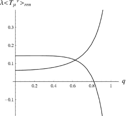
Figure 1: This graph shows behavior of the rescaled components of $\langle T_{t}^{t}\rangle_{ren}^{(1/2)}$ and $\langle T_{\theta}^{\theta}\rangle_{ren}^{(1/2)}$ [$\lambda=5760\pi^{2}m^{2}M_{H}^{6}$] of the renormalized stress- energy tensor of the quantized massive spinor field at the event horizon. The time component is always positive and increases with $q,$ whereas the angular component is positive for $q<0.823.$ For the extremal configuration $\lambda\langle T_{t}^{t}\rangle_{ren}^{(1/2)}=5.907$ and $\lambda\langle T_{\theta}^{\theta}\rangle_{ren}^{(1/2)}=-8.843.$

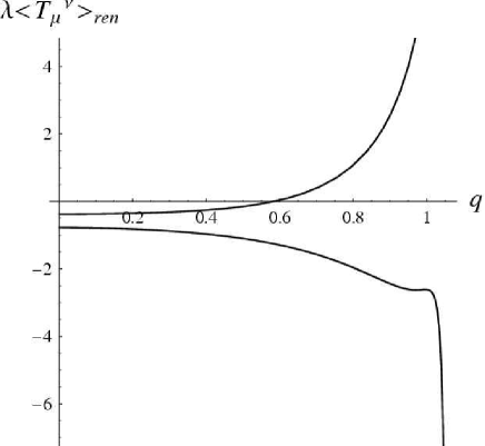
Figure 2: This graph shows behavior of the rescaled components of $\langle T_{t}^{t}\rangle_{ren}^{(1)}$ and $\langle T_{\theta}^{\theta}\rangle_{ren}^{(1)}$ [$\lambda=5760\pi^{2}m^{2}M_{H}^{6}$]of the renormalized stress- energy tensor of the quantized massive vector field at the event horizon. The time component increases with $q$ and is negative for $q<0.581.$ For the extremal configuration $\lambda\langle T_{t}^{t}\rangle_{ren}^{(1)}=35.080$ and $\lambda\langle T_{\theta}^{\theta}\rangle_{ren}^{(1)}=-52.990$

First, let us consider the horizon values of the components of $\langle T_{\mu}^{\nu}\rangle_{ren}^{\left(s\right)}.$ Spherical symmetry and regularity impose severe constrains on the structure of the stress-energy tensor at the event horizon. It suffices, therefore, to consider only its two independent components, say, $\langle T_{t}^{t}\rangle_{ren}^{\left(s\right)}$ and $\langle T_{\theta}^{\theta}\rangle_{ren}^{\left(s\right)}.$ The run of this components as functions of $q$ is exhibited in Figs. 1 and 2, for spinor and vector fields, respectively.

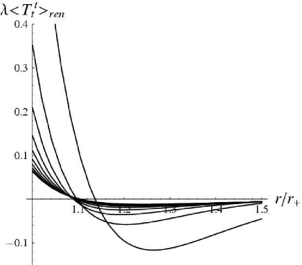
Figure 3: This graph shows the radial dependence of the rescaled component $\langle T_{t}^{t}\rangle_{ren}^{(1/2)}$ [$\lambda=5760\pi^{2}m^{2}M_{H}^{6}$] of the stress-energy tensor of the quantized massive spinor field in the spacetime of the ABGB black hole. From top to bottom at the event horizon the curves are plotted for $q=1-i/10,$ $(i=0,1,...,9).$ Each curve attains a negative minimum in the vicinity of $r_{+}.$

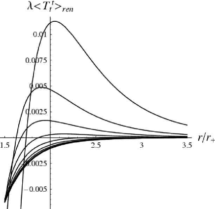
Figure 4: This graph shows the radial dependence of the rescaled component $\langle T_{t}^{t}\rangle_{ren}^{(1/2)}$ [$\lambda=5760\pi^{2}m^{2}M_{H}^{6}$] of the stress-energy tensor of the quantized massive spinor field in the spacetime of the ABGB black hole for $1.5<r/r_{+}<3.5$. From top to bottom the curves are plotted for $q=1-i/10,$ $(i=0,...,9)$

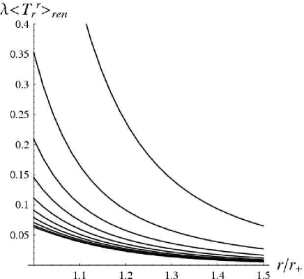
Figure 5: This graph shows the radial dependence of the rescaled component $\langle T_{r}^{r}\rangle_{ren}^{(1/2)}$ [$\lambda=5760\pi^{2}m^{2}M_{H}^{6}$] of the stress-energy tensor of the quantized massive spinor field in the spacetime of the ABGB black hole. From top to bottom the curves are plotted for $q=1-i/10,$ $(i=0,...,9).$ Each curve decreases monotonically to $0^{+}$ with $r.$

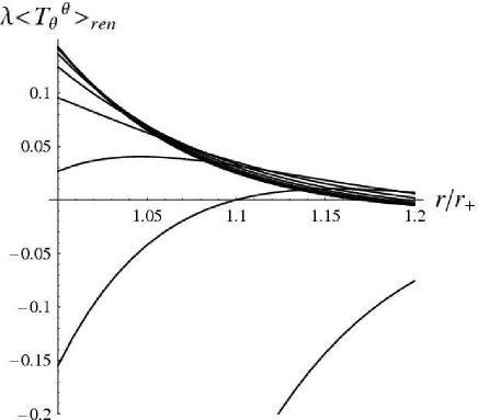
Figure 6: This graph shows the radial dependence of the rescaled component $\langle T_{\theta}^{\theta}\rangle_{ren}^{(1/2)}$ [$\lambda=5760\pi^{2}m^{2}M_{H}^{6}$] of the stress-energy tensor of the quantized massive spinor field in the spacetime of the ABGB black hole. From top to bottom at the event horizon the curves are plotted for $q=i/10,$ $(i=1,...,10).$ For $q<0.823$ the component $\langle T_{\theta}^{\theta}\rangle_{ren}^{(1/2)}$ is positive in the vicinity of the event horizon.

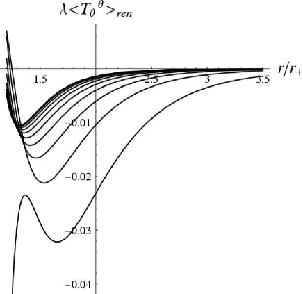
Figure 7: This graph shows the radial dependence of the rescaled component $\langle T_{\theta}^{\theta}\rangle_{ren}^{(1/2)}$ [$\lambda=5760\pi^{2}m^{2}M_{H}^{6}$] of the stress-energy tensor of the quantized massive spinor field in the spacetime of the ABGB black hole for $1.2<r/r_{+}<3.5.$ From top to bottom (in the minima) the functions are plotted for $q=i/10,$ $(i=1,...,10).$

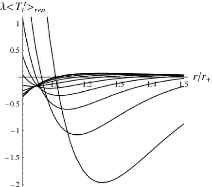
Figure 8: This graph shows the radial dependence of the rescaled component $\langle T_{t}^{t}\rangle_{ren}^{(1)}$ [$\lambda=5760\pi^{2}m^{2}M_{H}^{6}$] of the stress-energy tensor of the quantized massive vector field in the spacetime of the ABGB black hole. At the event horizon $\langle T_{t}^{t}\rangle_{ren}^{(1)}$ is positive for $q>0.851.$ For $q<0.465$ the curves reach minimum.

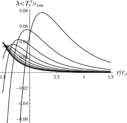
Figure 9: This graph shows the radial dependence of the rescaled component $\langle T_{t}^{t}\rangle_{ren}^{(1)}$ [$\lambda=5760\pi^{2}m^{2}M_{H}^{6}$] of the stress-energy tensor of the quantized massive vector field in the spacetime of the ABGB black hole. From top to bottom (at $r=2.5r_{+}$) horizon the curves are plotted for $q=1-i/10,$ $(i=0,...,9).$

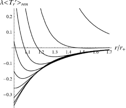
Figure 10: This graph shows the radial dependence of the rescaled component $\langle T_{r}^{r}\rangle_{ren}^{(1)}$ [$\lambda=5760\pi^{2}m^{2}M_{H}^{6}$] of the stress-energy tensor of the quantized massive vector field in the spacetime of the ABGB black hole. From top to bottom at the event horizon the curves are plotted for $q=1-i/10,$ $(i=0,...,9).$ For $q<0.387$ $\langle T_{r}^{r}\rangle_{ren}^{(1)}$ increases with $r$ to $0^{-}$ whereas for $q>0.919$ it is a monotonically decreasing function.

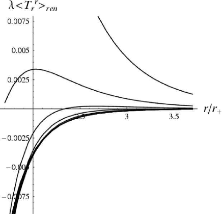
Figure 11: This graph shows the radial dependence of the rescaled component $\langle T_{r}^{r}\rangle_{ren}^{(1)}$ [$\lambda=5760\pi^{2}m^{2}M_{H}^{6}$] of the stress-energy tensor of the quantized massive vector field in the spacetime of the ABGB black hole for $1.7<r/r_{+}<3.7$

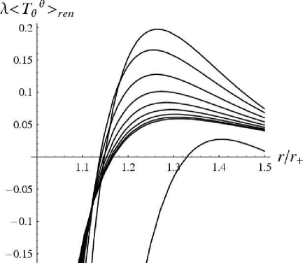
Figure 12: This graph shows the radial dependence of the rescaled component $\langle T_{\theta}^{\theta}\rangle_{ren}^{(1)}$ [$\lambda=5760\pi^{2}m^{2}M_{H}^{6}$] of the stress-energy tensor of the quantized massive vector field in the spacetime of the ABGB black hole. It is always negative at the event horizon and increases to a local maximum. From top to bottom the curves are for $q=1-i/10,$ $(i=1,...,9)$ and $q=1.$

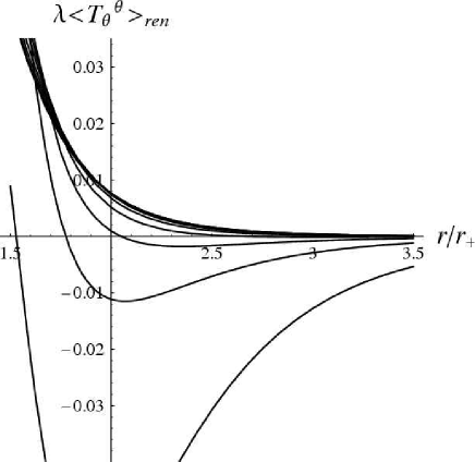
Figure 13: This graph shows the radial dependence of the rescaled component $\langle T_{\theta}^{\theta}\rangle_{ren}^{(1)}$ [$\lambda=5760\pi^{2}m^{2}M_{H}^{6}$] of the stress-energy tensor of the quantized massive vector field in the spacetime of the ABGB black hole. For $q<0.534$ it decreases monotonically to $0^{+};$ for $q>0.534$ it has a local minimum and increases to $0^{-}.$

The run of the stress-energy tensor for a several exemplary values of $q$ is exhibited in Figs. 3-13. Each curve represents the radial dependence of the rescaled component of $\langle T_{\mu}^{\nu}\rangle_{ren}^{\left(s\right)}$ for a given $q.$ We shall start our discussion of the numerical results with the spin-$1/2$ field. First, observe that the energy density $\rho^{\left(1/2\right)}\left(\rho^{\left(s\right)}=-\langle T_{t}^{t}\rangle_{ren}^{\left(s\right)}\right)$ is always negative at the event horizon, and, thus, by continuity, it is negative in its vicinity. Further $\rho^{\left(1/2\right)}$ attains a positive local maximum as can be clearly seen in Fig 3. For $q>1/\sqrt{5}$ the energy density develops a negative minium (Fig. 4) and goes to $0^{-\text{ }}$as $r\rightarrow\infty$. Further, inspection of the leading behavior of Eq. (58) shows that $\rho^{\left(1/2\right)}$ is positive at large distances for $q<1/\sqrt{5.}$

The radial pressure $p_{r}^{\left(1/2\right)}$ $(p_{r}^{\left(s\right)}=\langle T_{r}^{r}\rangle_{ren}^{\left(s\right)})$ is positive at the event horizon and $p_{r}^{\left(1/2\right)}\left(r_{+}\right)=-\rho^{\left(1/2\right)}$ $\left(r_{+}\right)$; subsequently, it decreases monotonically to $0^{+}$ with $r$. The behavior of $p_{r}^{\left(1/2\right)}$ is plotted in Fig. 5.

The tangential pressure, $p_{\theta}^{\left(1/2\right)}\left(p_{\theta}^{\left(s\right)}=\langle T_{\theta}^{\theta}\rangle_{ren}^{\left(s\right)}\right)$ is plotted in Figs. 6 and 7. At the event horizon it is positive for $q<0.823$, approaches a negative minimum at $r/r_{+}\approx 1.5$ and goes to $0^{-\text{ }}$ as $r\rightarrow\infty.$ A closer examination indicates that for $q>0.756,$ it develops a local maximum, which disappears near the extremality limit.

In general, there are no qualitative similarities between components of the renormalized stress-enegy tensor of the massive spinor and vector fields, as can be easily seen in Figs. 8-13. In the vicinity of the event horizon the energy density of the massive vector field is positive for $q<0.581$ and negative otherwise. For $q>0.465$ the energy density approaches a maximum, and, subsequently, regardless of $q$ it has a minimum. As the leading behavior as $r\rightarrow\infty$ is governed by the first term in rhs of (72), $p_{t}^{\left(1\right)}\rightarrow 0^{-}.$ Other qualitative and quantitative features of the energy density can easily be inferred from Figs. 8 and 9.

Numerical calculations indicate that for $q<0.387$ the radial pressure, $p_{r}^{\left(1\right)},$ is negative and monotonically increases to $0^{-}$ as $r$ $\rightarrow\infty.$ For $0.387<q<$ $0.919$ there appears a local minimum in the closest neighborhood of the event horizon, and, for $0.534<q<0.919$ , the radial pressure approaches a local maximum. Finally, for $q>0.919$, it decreases monotonically to $0^{+}.$ The run of $p_{r}^{\left(1\right)}$ for a few exemplary values of $q$ is plotted in Figs. 10 and 11.

The tangential pressure of the vector field is negative on the event horizon and increases to a global maximum. Subsequent behavior of $p_{\theta}^{\left(1\right)}$ depends on $q$: it decreases monotonically to $0^{+\text{ }}$ for $q<0.534$ whereas for $q>0.534$ the tangential pressure has a local minimum and increases to $0^{-}.$ Some other qualitative and quantitative features, as for example the numerical values of $p_{\theta}^{\left(1\right)}$ at the maxima and minima can easily be inferred from Figs. 12 and 13.

The numerical calculations carried out in the external region of the extremal configuration shows that the run of the stress-energy tensor qualitatively follows the analogous behavior for $q=1$ case, and, consequently, it will not be discussed separately.

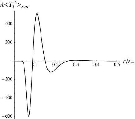
Figure 14: This graph shows the radial dependence of the rescaled component $\langle T_{t}^{t}\rangle_{ren}^{(1)}$ [$\lambda=m^{2}M_{H}^{6}$] of the stress-energy tensor of the quantized massive spinor field inside the event horizon of the extreme ABGB black hole.

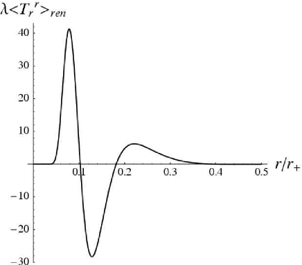
Figure 15: This graph shows the radial dependence of the rescaled component $\langle T_{r}^{r}\rangle_{ren}^{(1)}$ [$\lambda=m^{2}M_{H}^{6}$] of the stress-energy tensor of the quantized massive spinor field inside the event horizon of the extreme ABGB black hole.

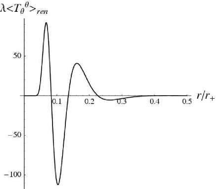
Figure 16: This graph shows the radial dependence of the rescaled component $\langle T_{\theta}^{\theta}\rangle_{ren}^{(1)}$ [$\lambda=m^{2}M_{H}^{6}$] of the stress-energy tensor of the quantized massive spinor field inside the event horizon of the extreme ABGB black hole.

Now, let us consider the vacuum polarization effects inside the event horizon of the extremal configuration. The run of the rescaled components of stress-energy tensor of the massive spinor field is exhibited in Figs 14-16. All the components display oscillatory behavior for $r/r_{+}>0.05,$ indicating that the back reaction effects would be especially interesting there. Such a behavior can easily be understood in relation with the behavior of the line element. Indeed, for small $r$ the line element closely resembles that of a flat spacetime, and, consequently, the vacuum polarization effects are small. On the other hand, for $r/r_{+}>0.05$ the function $f(r)$ changes noticeably leading to the changes of the stress-energy tensor. The competition of the local geometric terms $\delta W_{i}/\delta g_{\mu\nu}$ lead to its oscillatory-like behavior. Numerical calculations indicate that the stress-energy tensor of the quantized vector field is qualitatively similar to that of the spinor field and approximately one has

$$\langle T_{\mu}^{\nu}\rangle_{ren}^{(1)}\approx 10\times\langle T_{\mu}^{\nu}\rangle_{ren}^{(1/2)}$$ (79)

The basic features of the stress-energy tensor of the quantized massive vector field can easily be infrred form Figs. 14-16 and the above relation.

V Final remarks

In this paper we have constructed the renormalized stress-energy tensor of the massive spinor and vector fields in the spacetime of ABGB black hole. The scalar case has been analyzed extensively in our two previous papers. The method employed here is based on the observation that the first-order effective action could be expressed in terms of the (traced) coincidence limit of the coefficient $a_{3}.$ Functional differentiation of this action with respect to the metric tensor yields the most general first-order (i.e. proportional to $m^{-2}$) stress-energy tensor. Such a generic tensors of the quantized massive scalar, spinor and vector fields have been constructed for the first time in Matyjasek (2000, 2001).

Application of our general formulas, although conceptually straightforward, is technically rather intricate, and produces quite complex results. Therefore, for clarity, we have analyzed the leading behavior of $\langle T_{\mu}^{\nu}\rangle_{ren}^{\left(s\right)}$ in some physically important regimes. This discussion has been supplemented with detailed numerical calculations. The results have also been used to construct and analyze the stress-energy tensor in $\mathrm{AdS}_{2}\times\mathrm{S}^{2},$ spaces, which are naturally related to the near horizon geometry of the extremal ABGB black hole.

A special emphasis in this paper has been put on the extremal configurations. Specifically, it has been shown that the stress-energy tensor of the massive fields is regular inside the degenerate event horizon. This result raises important question of the nature of the black hole interior in the back-reaction problem. Preliminary calculations carried out in Berej et al. (2006) for the quadratic gravity, which, for certain calculational purposes, may be considered as some sort of a toy model of the semi-classical theory, indicate that at least for the first-order calculations it is possible to obtain regular solution, at the expense of a small modification of the classical nonlinear action. Of course, the stress-energy tensor of the quantized massive fields constructed in the general static, spherically symmetric and asymptotically flat spacetime is far more complicated than quadratic terms Berej et al. (2006), however, the general pattern that lies behind the calculations should be, in general, the same. The calculations carried out so far indicate that this is indeed the case, although lengthy and complicated results expressed in term of the polylogarithms are rather hard to analyze and manipulate. Moreover, it would be interesting to investigate the back reaction problem for any $q$ outside the event horizon. Finally, observe that the ABGB solution with the cosmological constant may provide an interesting setting for studying the influence of the quantized fields upon ultraextremal horizons. These problems are being studied and the results will be reported elsewhere.

.

References

- Birrell and Davies (1982) N. D. Birrell and P. C. W. Davies, Quantum fields in curved space (Cambridge Unversity Press, Cambridge, 1982).
- Schwinger (1951) J. S. Schwinger, Phys. Rev. 82, 664 (1951).
- DeWitt (1975) B. S. DeWitt, Phys. Reps. 19, 295 (1975).
- Barvinsky and Vilkovisky (1985) A. O. Barvinsky and G. A. Vilkovisky, Phys. Rept. 119, 1 (1985).
- Frolov and Zelnikov (1982) V. P. Frolov and A. I. Zelnikov, Phys. Lett. 115B, 372 (1982).
- Frolov and Zelnikov (1983) V. P. Frolov and A. I. Zelnikov, Phys. Lett. 123B, 197 (1983).
- Frolov and Zelnikov (1984) V. P. Frolov and A. I. Zelnikov, Phys. Rev. D29, 1057 (1984).
- Matyjasek (2000) J. Matyjasek, Phys. Rev. D61, 124019 (2000), eprint gr-qc/9912020.
- Matyjasek (2001) J. Matyjasek, Phys. Rev. D63, 084004 (2001), eprint gr-qc/0010097.
- Anderson et al. (1993) P. R. Anderson, W. A. Hiscock, and D. A. Samuel, Phys. Rev. Lett. 70, 1739 (1993).
- Anderson et al. (1995) P. R. Anderson, W. A. Hiscock, and D. A. Samuel, Phys. Rev. D51, 4337 (1995).
- Popov (2003) A. A. Popov, Phys. Rev. D67, 044021 (2003), eprint hep-th/0302039.
- Hiscock et al. (1997) W. A. Hiscock, S. L. Larson, and P. R. Anderson, Phys. Rev. D56, 3571 (1997), eprint gr-qc/9701004.
- Taylor et al. (1997) B. E. Taylor, W. A. Hiscock, and P. R. Anderson, Phys. Rev. D55, 6116 (1997), eprint gr-qc/9608036.
- Taylor et al. (2000) B. E. Taylor, W. A. Hiscock, and P. R. Anderson, Phys. Rev. D61, 084021 (2000), eprint gr-qc/9911119.
- Matyjasek (2003) J. Matyjasek, Acta Phys. Polon. B34, 3921 (2003), eprint gr-qc/0210070.
- Matyjasek and Zaslavskii (2001) J. Matyjasek and O. B. Zaslavskii, Phys. Rev. D64, 104018 (2001), eprint gr-qc/0102109.
- Berej and Matyjasek (2003) W. Berej and J. Matyjasek, Acta Phys. Polon. B34, 3957 (2003).
- Matyjasek and Zaslavskii (2005) J. Matyjasek and O. B. Zaslavskii, Phys. Rev. D71, 087501 (2005), eprint gr-qc/0502115.
- Berej and Matyjasek (2002) W. Berej and J. Matyjasek, Phys. Rev. D66, 024022 (2002), eprint gr-qc/0204031.
- Sakharov (1966) A. D. Sakharov, Sov. Phys. JETP 22, 21 (1966).
- Gliner (1966) E. B. Gliner, Sov. Phys. JETP 22, 378 (1966).
- Bardeen (1968) J. M. Bardeen, in GR 5 Proceedings (Tbilisi, 1968).
- Frolov et al. (1989) V. P. Frolov, M. A. Markov, and V. F. Mukhanov, Phys. Lett. B216, 272 (1989).
- Frolov et al. (1990) V. P. Frolov, M. A. Markov, and V. F. Mukhanov, Phys. Rev. D41, 383 (1990).
- Zaslavskii (2004) O. B. Zaslavskii, Phys. Rev. D70, 104017 (2004), eprint gr-qc/0410101.
- Dymnikova (1992) I. Dymnikova, Gen. Rel. Grav. 24, 235 (1992).
- Dymnikova (2003) I. Dymnikova, Int. J. Mod. Phys. D12, 1015 (2003), eprint gr-qc/0304110.
- Borde (1997) A. Borde, Phys. Rev. D55, 7615 (1997), eprint gr-qc/9612057.
- Mars et al. (1996) M. Mars, M. M. Martín-Prats, and J. M. M. Senovilla, Classical Quantum Gravity 13, L51 (1996).
- Ayon-Beato and Garcia (2000) E. Ayon-Beato and A. Garcia, Phys. Lett. B493, 149 (2000), eprint gr-qc/0009077.
- Ayon-Beato and Garcia (2005) E. Ayon-Beato and A. Garcia, Gen. Rel. Grav. 37, 635 (2005), eprint hep-th/0403229.
- Ayon-Beato and Garcia (1999) E. Ayon-Beato and A. Garcia, Phys. Lett. B464, 25 (1999), eprint hep-th/9911174.
- Bronnikov (2000) K. A. Bronnikov, Phys. Rev. Lett. 85, 4641 (2000).
- Bronnikov (2001) K. A. Bronnikov, Phys. Rev. D63, 044005 (2001), eprint gr-qc/0006014.
- Gilkey (1975) P. B. Gilkey, J. Differential Geometry 10, 601 (1975).
- Avramidi (1991) I. G. Avramidi, Nucl. Phys. B355, 712 (1991).
- Avramidi (1986) I. G. Avramidi (1986), eprint hep-th/9510140.
- Corless et al. (1996) R. M. Corless, G. H. Gonnet, D. E. G. Hare, D. J. Jeffrey, and D. E. Knuth, Adv. Comput. Math. 5, 329 (1996).
- Decanini and Folacci (0600) Y. Decanini and A. Folacci (0600), eprint arXiv:0706.0691 [gr-qc].
- Bertotti (1959) B. Bertotti, Phys. Rev. 116, 1331 (1959).
- Robinson (1959) I. Robinson, Bull. Acad. Polon. 7, 351 (1959).
- Kofman and Sahni (1983) L. A. Kofman and V. Sahni, Phys. Lett. 127B, 197 (1983).
- Bardeen and Horowitz (1999) J. M. Bardeen and G. T. Horowitz, Phys. Rev. D60, 104030 (1999), eprint hep-th/9905099.
- Zaslavskii (1997) O. B. Zaslavskii, Phys. Rev. D56, 2188 (1997), eprint gr-qc/9707015.
- Solodukhin (1999) S. N. Solodukhin, Phys. Lett. B448, 209 (1999), eprint hep-th/9808132.
- Dias and Lemos (2003) O. J. C. Dias and J. P. S. Lemos, Phys. Rev. D68, 104010 (2003), eprint hep-th/0306194.
- Cardoso et al. (2004) V. Cardoso, O. J. C. Dias, and J. P. S. Lemos, Phys. Rev. D70, 024002 (2004), eprint hep-th/0401192.
- Dadhich (2000) N. Dadhich, On product spacetime with 2-sphere of constant curvature (2000), eprint gr-qc/0003026.
- Caldarelli et al. (0400) M. Caldarelli, L. Vanzo, and S. Zerbini (0400), eprint hep-th/0008136.
- Matyjasek (2004) J. Matyjasek, Phys. Rev. D70, 047504 (2004), eprint gr-qc/0403109.
- (52) J. Matyjasek and A. A. Popov, unpublished.
- Berej et al. (2006) W. Berej, J. Matyjasek, D. Tryniecki, and M. Woronowicz, Gen. Rel. Grav. 38, 885 (2006), eprint hep-th/0606185.