Reconciling Semiclassical and Bohmian Mechanics:
II. Scattering states for discontinuous potentials

Abstract

In a previous paper [J. Chem. Phys. 121 4501 (2004)] a unique bipolar decomposition, $\Psi=\Psi_{1}+\Psi_{2}$ was presented for stationary bound states $\Psi$ of the one-dimensional Schrödinger equation, such that the components $\Psi_{1}$ and $\Psi_{2}$ approach their semiclassical WKB analogs in the large action limit. Moreover, by applying the Madelung-Bohm ansatz to the components rather than to $\Psi$ itself, the resultant bipolar Bohmian mechanical formulation satisfies the correspondence principle. As a result, the bipolar quantum trajectories are classical-like and well-behaved, even when $\Psi$ has many nodes, or is wildly oscillatory. In this paper, the previous decomposition scheme is modified in order to achieve the same desirable properties for stationary scattering states. Discontinuous potential systems are considered (hard wall, step, square barrier/well), for which the bipolar quantum potential is found to be zero everywhere, except at the discontinuities. This approach leads to an exact numerical method for computing stationary scattering states of any desired boundary conditions, and reflection and transmission probabilities. The continuous potential case will be considered in a future publication.

I INTRODUCTION

Much attention has been directed by theoretical/computational chemists towards developing reliable and accurate means for solving dynamical quantum mechanics problems—i.e., for obtaining solutions to the time-dependent Schrödinger equation—for molecular systems. Insofar as “exact” quantum methods are concerned, two traditional approaches have been used: (1) representation of the system Hamiltonian in a finite, direct-product basis set; (2) discretization of the wavefunction onto a rectilinear grid of lattice points over the relevant region of configuration space. Both approaches, however, suffer from the drawback that the computational effort scales exponentially with system dimensionality.bowman86 ; bacic89 Recently, a number of promising new methods have emerged with the potential to alleviate the exponential scaling problem once and for all. These include various basis set optimization methods,poirier99qcII ; poirier00gssI ; yu02b ; wangx03b and build-and-prune methods,dawes04 such as those based on wavelet techniques.poirier03weylI ; poirier04weylII ; poirier04weylIII

On the other hand, a completely different approach to the exponential scaling problem is to use basis sets or grid points, that themselves evolve over time. The idea is that at any given point in time, one need sample a much smaller Hilbert subspace, or configuration space region, than would be required at all times—thus substantially reducing the size of the calculation. For basis set calculations, much progress along these lines has been achieved by the multi-configurational time-dependent Hartree (MCTDH) method, developed by Meyer, Manthe and co-workers.meyer90 ; manthe92 More recently, time-evolving grid, or “quantum trajectory” methodslopreore99 ; mayor99 ; wyatt99 ; wyatt01b ; wyatt01c ; wyatt (QTMs) have also been developed, and for certain types of systems, successfully applied at quite high dimensionalities.wyatt01c ; wyatt

QTMs are based on the hydrodynamical picture of quantum mechanics, developed over half a century ago by Bohmbohm52a ; bohm52b and Takabayasi,takabayasi54 who built on the earlier work of Madelungmadelung26 and van Vleck.vanvleck28 QTMs are inherently appealing for a number of reasons. First, they offer an intuitive, classical-like understanding of the underlying dynamics, which is difficult-to-impossible to extract from more traditional fixed grid/basis methods. In effect, quantum trajectories are like ordinary classical trajectories, except that they evolve under a modified potential $V+Q$, where $Q$ is the wavefunction-dependent “quantum potential” correction. Second, QTMs hold the promise of delivering exact quantum mechanical results without exponential scaling in computational effort. Third, they provide a pedagogical understanding of entirely quantum mechanical effects such as tunnelinglopreore99 ; wyatt and interference.poirier04bohmI ; zhao03 They have already been used to solve a variety of different types of problems, including barrier transmission,lopreore99 non-adiabatic dynamics,wyatt01 and mode relaxation.bittner02b Several intriguing phase space generalizations have also emerged,takabayasi54 ; shalashilin00 ; burghardt01a ; burghardt01b of particular relevance for dissipative systems.trahan03b ; donoso02 ; bittner02a ; hughes04

Despite this success, QTMs suffer from a significant numerical drawback, which, to date, precludes a completely robust application of these methods. Namely: QTMs are numerically unstable in the vicinity of amplitude nodes. This “node problem” manifests in several different ways:wyatt01b ; wyatt (1) infinite forces, giving rise to kinky, erratic trajectories; (2) compression/inflation of trajectories near wavefunction local extrema/nodes, leading to; (3) insufficient sampling for accurate derivative evaluations. Nodes are usefully divided into two categories,poirier04bohmI depending on whether $Q$ is formally well-behaved (“type one” nodes) or singular (“type two” nodes). For stationary state solutions to the Schrödinger equation, for instance, all nodes are type one nodes. In principle, type one nodes are “gentler” than type two nodes; however, from a numerical standpoint, even type one nodes will give rise to the problems listed above, because the slightest numerical error in the evaluation of $Q$ is sufficient to cause instability.

In the best case, the node problem simply results in substantially more trajectories and time steps than the corresponding classical calculation; in the worst case, the QTM calculation may fail altogether, beyond a certain point in time. Several numerical methods, both “exact” and approximate, are currently being developed to deal with this important problem. The latter category includes the artificial viscositykendrick03 ; pauler04 and linearized quantum force methods,garashchuk04 both of which have proven to be very stable. While such approximate methods may not capture the hydrodynamic fields with complete accuracy in nodal regions, they do allow for continued evolution and long-time solutions, often unattainable via use of a traditional QTM. The “exact” methods include the adaptive hybrid methods,hughes03 and the complex amplitude method.garashchuk04b In the adaptive hybrid methods, for which hydrodynamic trajectories are evolved everywhere except for in nodal regions, where the time-dependent Schrodinger equation is solved instead to avoid node problems. Although they have been applied successfully for some problems, these methods are difficult to implement numerically, since not only must the hydrodynamic fields be somehow monitored for forming singularities, but there must also be an accurate means for interfacing and coupling the two completely different equations of motion. The complex amplitude method is cleaner to implement, but is only exact for linear and quadratic Hamiltonians.

In a recent paper,poirier04bohmI hereinafter referred to as “paper I,” one of the authors (Poirier) introduced a new strategy for dealing with the node problem, based on a bipolar decomposition of the wavefunction. The idea is to partition the wavefunction into two (or in principle, more) component functions, i.e. $\Psi=\Psi_{1}+\Psi_{2}$. One then applies QTM propagation separately to $\Psi_{1}$ and $\Psi_{2}$, which can be linearly superposed to generate $\Psi$ itself at any desired later time. In essence, this works because the Schrödinger equation itself is linear, but the equivalent Bohmian mechanical, or quantum Hamilton’s equations of motion (QHEM) are not.poirier04bohmI In principle, therefore, one may improve the numerical performance of QTM calculations simply by judiciously dividing up the initial wavepacket into pieces.

Although bipolar decompositions have been around for quite some time,floyd94 ; brown02 their use as a tool for circumventing the node problem for QTM calculations is quite recent. Two promising new exact methods that seek to accomplish this are the so-called “counter-propagating wave” method (CPWM),poirier04bohmI and the “covering function” method (CFM).babyuk04 In the CPWM, the bipolar decomposition is chosen to correspond to the semiclassical WKB approximation,poirier04bohmI for which all of the hydrodynamic field functions are smooth and classical-like, and the component wavefunctions are node-free. Interference is achieved naturally, via the superposition of left- and right-traveling (i.e. positive- and negative-momentum) waves. For one-dimensional (1D) stationary bound states, it can be shown that the resultant bipolar quantum potential $q(x)$ becomes arbitrarily small in the large action limit, even though the number of nodes becomes arbitrarily large. (Note: in accord with the convention established in LABEL:poirier04bohmI, upper/lower case will be used to denote the unipolar/bipolar field quantities). In the CFM, the idea is to superpose some well-behaved large-amplitude wave, with the actual ill-behaved (nodal or wildly oscillatory) wave, so as to “dilute” the undesirable numerical ramifications of the latter.

This paper is the second in a series designed to explore the CPWM approach, introduced in paper I. As discussed there in greater detail, there are many motivations for this approach, but the primary one is to reconcile the semiclassical and Bohmian theories, in a manner that preserves the best features of both, and also satisfies the correspondence principle. For our purposes, this means that the Lagrangian manifolds (LMs) for the two theories should become identical in the large action limit (Sec. II.2). As described above, a key benefit of the CPWM decomposition is an elegant treatment of interference, the chief source of nodes and “quasi-nodes”wyatt (i.e. rapid oscillations) in quantum mechanical systems. An interesting perspective on the role of interference in semiclassical and Bohmian contexts is to be found in a recent article by Zhao and Makri.zhao03

Whereas paper I focused on stationary bound states for 1D systems, the present paper (paper II) and the next in the series (paper III)poirier05bohmIII concern themselves with stationary scattering states. The CPWM decomposition of paper I is uniquely specified for any arbitrary 1D state—bound or scattering—and in the bound case, always satisfies the correspondence principle. However, the non-$L^{2}$ nature of the scattering states is such that the paper I decomposition generally does not satisfy the correspondence principle in this case. Simply put, the quantum trajectories and LMs exhibit oscillatory behavior in at least one asymptotic region (thereby manifesting reflection), whereas the semiclassical LMs do not. This is not a limitation of the CPWM, but is rather due to the fundamental failure of the basic WKB approximation to predict any reflection whatsoever for above-barrier energies, as has been previously well established.berry72 ; froman ; heading In semiclassical theory, a modification must therefore be made to the basic WKB approximation, in order to obtain meaningful scattering quantities. As discussed in Sec. II.2 and in paper III, our approach will be to apply a similar modification to the exact quantum decomposition (actually, a reverse modification) such that the correspondence principle remains satisfied, and the two theories thus reconciled, even for scattering systems.

It will be shown the modified CPWM gives rise to bipolar Bohmian LMs that are identical to the semiclassical LMs, regardless of whether or not the action is large. Put another way, this means that the bipolar quantum potentials $q$ effectively vanish, so that the resultant quantum trajectory evolution is completely classical. Moreover, the resultant component wavefunctions, $\Psi_{1}(x)$ and $\Psi_{2}(x)$, correspond asymptotically to the familiar “incident,” “transmitted,” and “reflected” waves of traditional scattering theory. Thus, the modified CPWM implementation of the bipolar Bohmian approach provides a natural generalization of these conceptually fundamental entities throughout all of configuration space, not just in the asymptotic regions, as is the case in conventional quantum scattering theory.

The above conclusions will be demonstrated for both discontinuous and continuous potential systems, in papers II and III, respectively. Discontinuous potentials—e.g. the hard wall, the step potential, and the square barrier/well—serve as a useful benchmark for the modified CPWM approach, because the scattering component waves (e.g. “incident wave,” etc.) in this case are well-defined throughout all of configuration space, according to a conventional scattering treatment. Although this is no longer true for continuous potentials, the foundation laid here in paper II can be extended to the continuous (and also time-dependent) case as well, as described in paper III. Additional motivation for the development of a scattering version of the CPWM, vis-a-vis the relevance for chemical physics applications, is provided in paper III. Additional motivation for the consideration of discontinuous potentials is provided in Sec. II.2 of the present paper.

II THEORY

II.1 Background

II.1.1 Bohmian mechanics

According to the Bohmian formulation,wyatt ; holland the QHEM are derived via substitution of the 1D (unipolar) wavefunction ansatz,

$$\Psi(x,t)=R(x,t)e^{iS(x,t)/\hbar}$$ (1)

into the time-dependent Schrödinger equation. For the 1D Hamiltonian,

$$\hat{H}=-{\hbar^{2}\over 2m}{\partial^{2}\over\partial x^{2}}+V(x),$$ (2)

this results in the coupled pair of nonlinear partial differential equations,

$$\frac{\partial S(x,t)}{\partial t} = -\frac{S^{\prime 2}}{2m}-V(x)+\frac{\hbar^{2}}{2m}\frac{R^{\prime\prime}}{R},$$

$$\frac{\partial R(x,t)}{\partial t} = -\frac{1}{m}R^{\prime}\,S^{\prime}-\frac{1}{2m}R\,S^{\prime\prime},$$ (3)

where $m$ is the mass, $V(x)$ is the system potential, and primes denote spatial partial differentiation.

The first of the two equations above is the quantum Hamilton-Jacobi equation (QHJE), whose last term is equal to $-Q(x,t)$, i.e. comprises the quantum potential correction. The second equation is a continuity equation. When combined with the quantum trajectory evolution equations, i.e.

$$P = m{dx\over dt}=S^{\prime},$$

$${dP\over dt} = -(V^{\prime}+Q^{\prime}),$$ (4)

the continuity equation ensures that the probability [i.e. density, $R(x,t)^{2}$, times volume element] carried by individual quantum trajectories is conserved over the course of their time evolution.

II.1.2 CPWM decomposition for stationary states

In paper I, we derived a unique bipolar decomposition,

$$\Psi(x)=\Psi_{+}(x)+\Psi_{-}(x),$$ (5)

for stationary eigenstates $\Psi(x)$ of 1D Hamiltonians of the Eq. (2) form, such that:

1. $\Psi_{\pm}(x)$ are themselves (non-$L^{2}$) solutions to the Schrödinger equation, with the same eigenvalue, $E$, as $\Psi(x)$ itself.

2. The invariant flux values, $\pm F$, of the two solutions, $\Psi_{\pm}(x)$, equal those of the two semiclassical (WKB) solutions.

3. The median of the enclosed action, $x_{0}$, equals that of the semiclassical solutions.

There are other important properties of the $\Psi_{\pm}(x)$,poirier04bohmI as discussed in Sec. I, and in LABEL:poirier04bohmI. Nevertheless, the above three conditions are sufficient to uniquely specify the decomposition. In the special case of bound (i.e. $L^{2}$) stationary states, the real-valuedness of $\Psi(x)$ implies that the $\Psi_{\pm}(x)$ are complex conjugates of each other.

II.2 Scattering systems

It is natural to ask to what extent the above analysis may be generalized for scattering potentials. Certainly, $\Psi(x)$ itself is no longer $L^{2}$, nor even real-valued, and there are generally two linearly independent solutions of interest for each $E$, instead of just one. Condition (1) above poses no difficulty for $\Psi_{\pm}(x)$, as these component functions are non-$L^{2}$ and complex-valued, even in the bound eigenstate case. In principle, condition (2) is not difficult either; although the flux value depends on the normalization of $\Psi$ itself, which is not $L^{2}$, certain well-established normalization conventions for scattering states exist, that can be applied equally well to semiclassical and exact quantum solutions. There is no action median per se for scattering states, as the action enclosed within the $\Psi_{+}(x)$ and $\Psi_{-}(x)$ phase space Lagrangian manifoldspoirier04bohmI ; keller60 ; maslov ; littlejohn92 (LMs) is infinite; however, the scattering analog of condition (3) is related to the asymptotic boundary conditions, and it is here that one encounters difficulty. Moreover, an additional concern is raised by the doubly-degenerate nature of the continuum eigenstates, namely: should each scattering $\Psi(x)$ have its own $\Psi_{\pm}(x)$ decomposition, or should there be a single $\Psi_{\pm}(x)$ pair, from which all degenerate $\Psi(x)$’s may be constructed via arbitrary linear superposition?

To resolve these issues, we will adopt the same general strategy used in paper I, i.e. we will resort to semiclassical theory as our guide, wherever possible. We will also exploit certain special features of the scattering problem not found in generic bound state systems, such as the asymptotic potential condition $V^{\prime}(x)\rightarrow 0$ as $x\rightarrow\pm\infty$ (where primes denote spatial differentiation), and its usual implications for scattering theory and applications.taylor

The basic WKB solutions are given by

$$\Psi_{\pm}^{\text{sc}}(x)=r_{\text{sc}}(x)e^{\pm is_{\text{sc}}(x)/\hbar},$$ (6)

where

$$r_{\text{sc}}(x)=\sqrt{{mF\over s^{\prime}_{\text{sc}}(x)}}\qquad\text{and}\qquad s^{\prime}_{\text{sc}}(x)=\sqrt{2m\left[{E-V(x)}\right]}$$ (7)

The corresponding positive and negative momentum functions, specifying the semiclassical LMs, are given by $p^{\text{sc}}_{\pm}(x)=\pm s^{\prime}_{\text{sc}}(x)$. Equations (6) and (7) apply to both bound and scattering cases; note that for both, $\Psi_{\pm}^{\text{sc}}(x)$ are complex conjugates of each other. The asymptotic potential condition ensures that these approach exact quantum plane waves asymptotically, with the usual scattering interpretations, i.e. $\Psi_{+}(x)$ in the $x\rightarrow-\infty$ asymptotic region is the incoming wave from the left (usually taken to be the incident wave), $\Psi_{+}(x)$ as $x\rightarrow\infty$ is the outgoing wave from the left (the usual transmitted wave), etc.

Insofar as determining the corresponding exact quantum solutions $\Psi_{\pm}(x)$, the procedure described in paper I is still appropriate for bound and semi-bound (i.e. on one side only) states, in that the results satisfy the correspondence principle globally, as desired (for semi-bound examples, consult the Appendix). For true scattering states, however, this procedure fails, in the sense that if $\Psi_{+}(x)$ is chosen to match the normalization and flux of $\Psi^{\text{sc}}_{+}(x)$ in the $x\rightarrow\infty$ asymptote, then it will necessarily approach a nontrivial linear superposition of $\Psi^{\text{sc}}_{+}(x)$ and $\Psi^{\text{sc}}_{-}(x)$ in the $x\rightarrow-\infty$ asymptote, and vice-versa. There is therefore an ambiguity as to how the corresponding quantum $\Psi_{\pm}(x)$’s should be defined, i.e. which asymptotic region should be used to effect the correspondence. More significantly though, either choice will result in component functions $\Psi_{\pm}(x)$ with substantial interference in one of the two asymptotic regions. This is due to partial reflection of the exact quantum scattering states, which is not predicted by the basic WKB approximation. Thus, in the large action limit, the exact quantum solutions manifest large-magnitude quantum potentials, $q_{\pm}(x)$, and rapidly oscillating field functions $q_{\pm}(x)$, $r_{\pm}(x)$, and $p_{\pm}(x)$—exactly the undesirable behavior that the CPWM was introduced to avoid—whereas the corresponding basic WKB functions are smooth, and asymptotically uniform.

The lack of any partial reflection is a well-understood shortcoming of the WKB approximationberry72 ; froman ; heading ; poirier03capI —i.e., the basic $\Psi_{\pm}^{\text{sc}}(x)$ components, though elegantly constructed from smooth classical functions $r_{\text{sc}}(x)$ and $s_{\text{sc}}(x)$, do not in and of themselves correspond to any actual quantum scattering solutions $\Psi(x)$. In light of the bipolar decomposition ideas introduced in paper I, however, our perspective is the reverse one: for any actual quantum $\Psi(x)$, can one determine an Eq. (5) decomposition such that the resultant $\Psi_{\pm}(x)$ resemble their well-behaved semiclassical counterparts, and is such a decomposition unique? Among other properties,poirier04bohmI the $\Psi_{\pm}(x)$ LM’s should become identical to the semiclassical LM’s in the large action limit, so as to satisfy the correspondence principle. Based on the considerations of the previous paragraph it is clear that the paper I decomposition does not achieve this goal, when applied to stationary scattering states.

We defer a full accounting of these issues—in the context of completely arbitrary continuous potentials $V(x)$—to paper III, wherein it will be demonstrated how to compute exact quantum reflection and transmission probabilities (and stationary scattering states) using only classical trajectories, and without the need for explicit numerical differentiation of the wavefunction. In the present paper, we lay the foundation for paper III, by focusing attention onto two key aspects whose development comprises an essential prerequisite.

First, as the paper III approach treats $V(x)$ as a sequence of steps,poirier05bohmIII the present paper II will focus exclusively on the step potential and related discontinuous potential systems, for which $V(x)=\text{const}$ in between successive steps. Discontinuous potentials are important for chemical physics, because they model steep repulsive wells, and are used in statistical theories of liquids. Moreover, they hold a special significance for QTM methods, for which they serve as a “worst-case scenario” benchmark. Indeed, conventional QTM techniques always fail when applied to discontinuous potentials. To date, The only such calculations that have been performedholland have computed the quantum potential from a completely separate time-dependent fixed-grid calculation (the “analytical approach”)wyatt rather than directly from the quantum trajectories themselves. Even if one could propagate trajectories for discontinous systems using a traditional QTM, the trajectories that would be generated would be very kinky and erratic,holland and a great many time trajectories and time steps would thus be required.

Second, since the new $\Psi_{\pm}(x)$ do not satisfy condition (1), unlike the paper I CPWM decomposition, the time evolution of these two component functions is clearly not that of the time-dependent Schrödinger equation. Moreover, since the $|\Psi_{\pm}|^{2}$ are constant over time [because $|\Psi|^{2}$ itself is stationary, and Eq. (5) is presumed unique], the two $\Psi_{\pm}(x,t)$ time evolutions must be coupled together. It is essential that the nature of this coupling be completely understood, in order that the present approach may be generalized to non-stationary state situations—e.g. to wavepacket scattering, as will be discussed in future publications. The ramifications for QTMs are equally important. Accordingly, the present paper focuses on the QTM propagation of the wavefunction and its bipolar components—with a keen eye towards generality and physical interpretation—even though the states involved are stationary. This approach leads to a pedagogically useful reinterpretation of “incident,” “transmitted,” and “reflected” waves—very reminiscent of ray optics in electromagnetic theory—which is applicable much more generally than traditional usage might suggest.

II.3 Basic applications

The necessary theory will be developed over the course of a consideration of various model application systems of increasing complexity.

II.3.1 free particle system

Let us first consider the simplest case imaginable, the free particle system, $V(x)=0$. In this case, the exact solutions $\Psi_{\pm}(x)=\Psi_{\pm}^{\text{sc}}(x)$ clearly satisfy the conditions of Sec. II.1.2, and the bipolar quantum potentials $q_{\pm}(x)$ are zero everywhere. Thus, the bipolar decomposition developed for bound states in paper I can be used directly with this continuum system, requiring only the slight modification that arbitrary linear combinations of $\Psi_{+}^{\text{sc}}(x)$ and $\Psi_{-}^{\text{sc}}(x)$ are to be allowed, in order to construct arbitrary scattering solutions $\Psi(x)$. For convenience, the linear combination coefficients will from here on out be directly incorporated into the amplitude functions, $r_{\pm}(x)$, and phase functions, $s_{\pm}(x)$, so that Eq. (5) is still correct.

If from all solutions $\Psi(x)$ one considers only that which satisfies the usual scattering boundary conditions (i.e. incident wave incoming from the left) then the negative momentum wave $\Psi_{-}$ vanishes, and $\Psi(x)=\Psi_{+}(x)$. There is zero reflection, and $100\%$ transmission. Put another way, the incident flux, $\lim_{x\rightarrow-\infty}j_{+}(x)$, is equal to the transmitted flux, $\lim_{x\rightarrow+\infty}j_{+}(x)$, where

$$j_{\pm}(x) = {\hbar\over 2im}\left[{\Psi_{\pm}^{*}(x){d\Psi_{\pm}(x)\over dx}-{d\Psi_{\pm}^{*}(x)\over dx}\Psi_{\pm}(x)}\right]$$ (8)

$$=\left[{p_{\pm}(x)\over m}\right]r_{\pm}^{2}(x),$$

[both flux values are equal to $F$, as in Eq. (7)].

In the quantum trajectory description, flux manifests as probability-transporting trajectories, which move along the LMs. For the boundary conditions described above, there are only positive momentum trajectories, moving uniformly from left to right with momentum $p_{+}(x)=\sqrt{2mE}$. If a $\Psi_{-}(x)$ contribution were present, its trajectories would move uniformly in the opposite direction [$p_{-}(x)=-\sqrt{2mE}$.] Since the two components $\Psi_{\pm}(x)$ are in this case uncoupled, the positive and negative momentum trajectories would have no interaction with each other.

II.3.2 hard wall system

We next consider the hard wall system:

$$V(x)={\cases{0&for $x\leq 0$;\cr\infty&for $x>0$.\cr}}$$ (9)

In the $x\leq 0$ region, the two $\Psi_{\pm}(x)$ components are exactly the same as in the free particle case, except that the $\Psi(0)=0$ boundary condition imposes the additional constraints,

$$s_{-}(0)=s_{+}(0)+\pi{\text{mod}}(2\pi)\qquad;\qquad r_{-}(0)=r_{+}(0).$$ (10)

This also results in only one linearly independent solution instead of two, i.e. $\Psi(x)\propto\sin(kx)$, with $k=\sqrt{2mE}/\hbar$. Regarding the LMs and trajectories, in the $x<0$ region, these are identical to those of Sec. II.3.1, e.g. the $\Psi_{+}(x)$ LM trajectories move uniformly to the right, towards the hard wall at $x=0$.

It is natural to ask what happens when the $\Psi_{+}(x)$ LM trajectories actually reach $x=0$. There are two reasonable interpretations. The first is that the trajectories keep moving uniformly into the $x>0$ region of configuration space. This approach treats the hard wall system as if it were the free particle system, but with the $x>0$ region effectively ignored.poirier00qcI This underscores the fact that unlike $\Psi(x)$ itself, the individual $\Psi_{\pm}(x)$ components per se are unconstrained at the origin—though the Eq. (10) constraint implies a unique correspondence between the two. This interpretation also makes it clear that for the hard wall system, the paper I decomposition is essentially identical to the present decomposition, as is worked out in detail in the Appendix.

In the second interpretation, the effect of the hard wall at $x=0$ is to cause instantaneous elastic reflection of a $\Psi_{+}(x)$ LM trajectory momentum, from $p=p_{+}=+\sqrt{2mE}$ to $p=p_{-}=-\sqrt{2mE}$. Afterwards, the reflected trajectory propagates uniformly backward, along the $\Psi_{-}(x)$ LM. In this interpretation, the trajectories never leave the allowed configuration space, $x\leq 0$. However, wavepacket reflection is essentially achieved via trajectory hopping from one LM to the other—not unlike that previously considered, e.g., in the context of non-adiabatic transitions.tully71 The trajectory hopping interpretation is adopted in the present paper, and in paper III, but the first interpretation will also be reconsidered in later publications. Note that for discontinuous potentials—and indeed more generallypoirier05bohmIII —one can regard trajectory hopping as the source of $\Psi_{\pm}(x)$ interaction coupling.

For the hard wall case, trajectory hopping only manifests at $x=0$, the sink of all $\Psi_{+}(x)$ LM trajectories, and the source of all $\Psi_{-}(x)$ LM trajectories. If these trajectories are to be regarded as one and the same via hopping, then a unique field transformation for $r$, $s$, and all spatial derivatives, must be specified. Fortunately, the unique correspondence between $\Psi_{+}(x)$ and $\Psi_{-}(x)$ described above, enables one to do just that. In particular, Eq. (10) specifies the correct transformations for $r$ and $s$, as transported by the quantum trajectories. All spatial derivatives of arbitrary orders can then be obtained via spatial differentiation of Eq. (6)—although in the hard wall case, only the $s^{\prime}$ condition, $p_{-}(0)=-p_{+}(0)$ is relevant, because all higher order derivatives are identically zero.

Since the magnitudes of the $p$ and $r$ fields associated with a given quantum trajectory are unchanged as a result of the trajectory hop, Eq. (8) implies that the incident and reflected flux values are the same (apart from sign), and so the scattering system exhibits 100% reflection and zero transmission (along each LM, the flux is invariantpoirier04bohmI ). These basic facts of the hard wall system are of course well understood. The point, though, is that we have now obtained the information in a time-dependent quantum trajectory manner, rather than through the usual route of applying boundary conditions to time-independent piecewise component functions. In other words, Eq. (10) now refers to individual quantum trajectories, rather than to wavefunctions.

This shift of emphasis is very important, and leads to quite a number of conceptual and computational advantages. For instance, the standard description of the hard wall stationary states would decompose these into plane wave components interpreted as “incident” and “reflected” waves. This language suggests a process, or change over time—i.e. a state that is initially incident, at some later time is somehow transformed into a reflected state. Nothing in the standard description, however, would seem to render transparent the usage of such terminology, i.e. $\Psi(x)$ is stationary, and so the reflected and transmitted components are in fact both present for all times. Of course, a localized superposition of stationary states, i.e. a wavepacket, may well exhibit such an explicit transformation over the course of the time evolution, as such a state is decidedly non-stationary. Indeed, wavepackets are relied upon by the more rigorous formulations of scattering theory, in order to justify the use of terms such as “reflected wave,” even in a stationary context.taylor Such formulations, though certainly legitimate, seem always to require a clever use of limits, the subtle distinction between unitary and isometric transformations, and other esoteric mathematical tricks.

On the other hand, the time-dependent bipolar quantum trajectory hopping picture presented above provides a physicality to such language that is immediately apparent. Over the course of the time evolution, although the wavefunction as a whole is stationary, each individual trajectory is first incident from the left, then collides with the hard wall, and is subsequently reflected back towards the left (i.e. towards $x\rightarrow-\infty$). The bipolar quantum trajectories are all classical, as the bipolar quantum potentials, $q_{\pm}(x)$, are zero everywhere except at the wall itself. Interference arises naturally from the superposition of the two LMs—i.e., from the trajectories that have already progressed to the point of reflecting, vs. those that have not reflected yet. In contrast, since $\Psi(x)$ itself exhibits very substantial interference, and an infinite number of nodes, the traditional unipolar QTM treatment would be very ill-behaved, i.e. $R(x)$ would oscillate wildly in the large $k$ limit, and $Q(x)$ would be numerically unstable near the nodes. Apart from these important pragmatic drawbacks, the incident/reflected interpretation of the quantum trajectories would also be lost.

The bipolar quantum trajectory description of the hard wall system is very reminiscent of ray optics, as used to describe the reflection of electromagnetic waves off of a perfectly reflecting surface.jackson Indeed, much can be gained from applying a ray optics analogy to quantum scattering applications, especially where discontinuous potentials are concerned. One can construct a simple gedankenexperiment as follows. Let $x_{L}<0$ denote some effective left edge of the system, well to the left of the interaction region. At some initial time $t=0$, all trajectories on the positive LM lying to the right of $x_{L}$ are ignored, as is the negative LM altogether. One then evolves the retained trajectories over time, and monitors the contribution that just these trajectories make to the total wavefunction. In some respects, it is as if the point $x_{L}$ were serving as the initial wavefront for some incoming wave, that at $t=0$ had not yet reached the hard wall/reflecting surface. Of course, if the actual wave were in fact truncated in this fashion, then the discontinuity in the field functions at the wavefront would result in a very non-trivial propagation over time, owing to the high-frequency components implicitly present. For actual waves, the precise nature of the wavefront is known to have a tremendous impact on the resultant dynamics.jackson ; brillouin14 We avoid such complicating details by always interpreting the “actual wave” to be the full stationary wave itself, i.e. the truncation is conceptual only.

In the ray optics analogy, the above situation is like a source of light located at $x_{L}$, which is suddenly “turned on” at $t=0$. It takes time for the wavefront to propagate to the reflecting surface, and additional time for the reflected wavefront to make its way back to $x=x_{L}$. Prior to the latter point in time, the evolution of the truncated electromagnetic wave is decidedly non-stationary; afterwards however, a stationary wave is achieved, at least within the region of interest, $x_{L}\leq x\leq 0$, as the wavefront has by this stage propagated beyond this region. The same qualitative comments apply to the bipolar quantum case, although of course the evolution equations are different.

A similar prescription may be used to achieve rudimentary “wavepacket dynamics,” even in the context of purely stationary states. Instead of retaining all initial trajectories that lie to the left of $x_{L}$, one retains only those that lie within some finite interval. The resulting time evolution is analogous to a light source that is turned on at $t=0$, and then turned off at some later time (prior to when the wavefront arrives at the reflecting surface). The initial “wavepacket” has uniform density, and moves with uniform speed towards the hard wall. Interference fringes then form after the foremost trajectories have been reflected onto the negative LM. Eventually, all trajectories within the interval are reflected, at which point interference ceases (the nodes are “healed”wyatt ), uniform density is restored, and the reflected wave travels with uniform speed in the reverse direction, back towards the starting point $x_{L}$. Qualitatively, this behavior is clearly similar to that undergone by actual wavepackets reflecting off of barrier potentials.

II.4 More complicated applications

The ideas described above can be easily extended to more complicated discontinuous potential systems, such as up- and down-step potentials, and any combination of multiple steps, e.g. square barriers and square wells. In paper III, they will even be extended to arbitrary continuous potentials.poirier05bohmIII In every case, the ray optics analogy from electromagnetic theory may also be extended accordingly. This approach provides a useful perspective on global reflection and transmission in scattering systems, and in particular, demonstrates how such quantities may be obtained from a single, universal expression for local reflection and transmission.

II.4.1 step potential system—above barrier energies

We next consider the step potential system:

$$V(x)={\cases{0&for $x\leq 0$;\cr V_{0}&for $x>0$,\cr}}$$ (11)

Classically, this system exhibits 100% transmission if the trajectory energy is above the barrier (i.e. $E>V_{0}$), and 100% reflection if the trajectory energy is below the barrier ($E<V_{0}$). Quantum mechanically, all above barrier trajectories are found to exhibit partial reflection and partial transmission, although there is a general increase in transmission probability with increasing energy. The below barrier quantum trajectories exhibit 100% reflection, as in the classical case; however, they also manifest tunneling into the classically forbidden $x>0$ region. Thus even quantum mechanically, the the above and below barrier cases must be handled somewhat differently.

To begin with, we consider the above-barrier case. Note that the LM’s are unbounded in either direction, i.e. the classically allowed region extends to both asymptotes, $x\rightarrow\pm\infty$. Incoming trajectories can therefore originate from either asymptote, thus giving rise to two linearly independent solutions, $\Psi(x)$. This is in stark contrast to the hard wall system, for which incoming trajectories could only originate from $x\rightarrow-\infty$, thus resulting in only one linearly independent solution for $\Psi(x)$.

In the standard time-independent picture, one starts with the four piecewise solutions,

$$\Psi_{A\pm}(x)=e^{\pm ip_{A}x/\hbar}\quad\text{and}\quad\Psi_{B\pm}(x)=e^{\pm ip_{B}x/\hbar},$$ (12)

where region $A$ corresponds to $x\leq 0$,region $B$ to $x\geq 0$. The momenta values are classical, i.e.

$$p_{A}=\sqrt{2mE}\quad\text{and}\quad p_{B}=\sqrt{2m(E-V_{0})}.$$ (13)

Matching $\Psi(x)$ and $\Psi^{\prime}(x)$ boundary conditions at $x=0$, and specifying asymptotic boundary conditions for $\Psi(x)$, then enables a unique determination of the four complex coefficients $A_{\pm}$ and $B_{\pm}$ in

$$\Psi(x)={\cases{A_{+}\Psi_{A+}(x)+A_{-}\Psi_{A-}(x)&for $x\leq 0$;\cr B_{+}\Psi_{B+}(x)+B_{-}\Psi_{B-}(x)&for $x\geq 0$,\cr}}.$$ (14)

In general, the solution coefficients depend on the particular stationary solution of interest. For the usual scattering convention of an incident wave incoming from the left (Fig. 1) the solutions are

$$A_{+}=1\quad \quad A_{-}=R=\left({p_{A}-p_{B}\over p_{A}+p_{B}}\right)$$ ;

$$B_{+}=T=\left({2p_{A}\over p_{A}+p_{B}}\right)\quad \quad B_{-}=0,$$ ; (15)

where $R$ and $T$ are respectively, reflection and transmission amplitudes. When flux is properly accounted for, the resultant reflection and transmission probababilities (which add up to unity) are given by

$$P_{\text{refl}}=|R|^{2}\qquad;\qquad P_{\text{trans}}=\left({p_{B}\over p_{A}}\right)|T|^{2}.$$ (16)

Note that Eqs. (15) and (16) above are correct for both an “up-step” and a “down-step”—i.e. for $V_{0}$ positive or negative. We can also apply these equations to the “opposite” boundary conditions, i.e. to an incident wave incoming from the right, by simply transposing $A$ and $B$ subscripts, and $+$ and $-$ subscripts ($p_{A}$ and $p_{B}$ are still positive). This is important, because any stationary solution $\Psi(x)$ can be obtained as some linear superposition of left-incident and right-incident solutions.

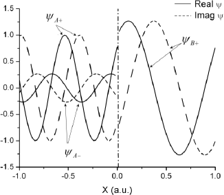
Figure 1: Component waves for a left-incident stationary eigenstate of the up-step barrier problem with $E>V_{0}$, as described in Sec. IV.1. Solid and dashed lines represent real and imaginary contributions, respectively. The dot-dashed line denotes the location of the step.

Regarding the time-dependent interpretation, it is evident that upon reaching the step discontinuity, left-incident trajectories must be partially reflected and partially transmitted. The trajectory is suddenly split into two, one that continues to propagate along the positive LM for the transmitted $B$ region (i.e. the $B+$ LM) and the other being instantaneously reflected down to the $A-$ LM. Moreover, since probability carried by individual quantum trajectories is conserved,wyatt ; holland this splitting must be done in a manner that preserves both probability and flux. In other words, the local splitting of the trajectory at $x=0$ must correspond to Eq. (15), which is now regarded as a local condition, giving rise to local reflection and transmission amplitudes, $R$ and $T$. For the present step potential case, these local quantities are directly related to the global $P_{\text{refl}}$ and $P_{\text{trans}}$ values via Eq. (16). For multiple step potentials (Sec. II.4.3), the global expressions above [Eq. (16)] no longer apply; however, a local, time-dependent trajectory version of Eq. (15) does turn out to be correct.

Such an expression, immediately applicable to all single and multiple step systems, can be written as follows:

$$r_{\text{refl}}=\left({p_{\text{i/r}}-p_{\text{trans}}\over p_{\text{i/r}}+p_{\text{trans}}}\right)r_{\text{inc}}\quad \quad s_{\text{refl}}=s_{\text{inc}}$$ ; (17)

$$r_{\text{trans}}=\left({2p_{\text{i/r}}\over p_{\text{i/r}}+p_{\text{trans}}}\right)r_{\text{inc}}\quad \quad s_{\text{trans}}=s_{\text{inc}}.$$ ; (18)

In the above equations, “inc” refers to any trajectory, locally incident on some particular step from some particular direction, which spawns both a locally reflected trajectory, “refl,” and a locally transmitted trajectory, “trans”. The quantity $p_{\text{i/r}}$ is the (positive) momentum associated with the locally incident/reflected trajectory; similarly, $p_{\text{trans}}$ (also positive) is associated with the locally transmitted trajectory. For above-barrier incident trajectories, note that the local reflection and transmission amplitudes are both real, thus ensuring the reality of $r$ and $s$ for the spawned trajectories.

Returning to the step potential system, the ray optics picture can once again shed some interesting light. The optical analog of the step is an interface between two media with different indices of refraction. Light incident on such an interface will partially reflect back towards the original source, and partially refract forwards into the new medium. The refraction is completely analogous to the discontinuous change in momentum, $(p_{B}-p_{A})$, that suddenly occurs as one crosses the step (Fig. 3). In any event, the ray optics gedankenexperiment described in Sec. II.3.2 can also be applied to the step potential system, in order to obtain a particular stationary solution $\Psi(x)$ with any desired boundary conditions.

For instance, suppose one is interesting in constructing the left-incident wave solution, i.e. that of Eq. (15). At $t=0$, only the $\Psi_{A+}$ wave is considered, and only those trajectories for which $x\leq x_{L}$, as before. As the incident trajectories reach the step, two new waves are dynamically created from the spawned trajectories: a transmitted wave traveling to the right, and a reflected wave traveling to the left. A plot of the overall density $|\Psi(x,t)|^{2}$ so obtained will change over time, as the transmitted and reflected wavefronts propagate into their respective regions (Fig. 6). Eventually, however, these wavefronts will propagate beyond the region of interest, i.e. $x_{L}\leq x\leq x_{R}$, where $x_{R}>0$ is the right edge of the region of interest. When this occurs, the solution for $\Psi(x)$ obtained within the region of interest will be exactly equal to the stationary solution with the desired boundary condition.

As in the hard wall case, one can also perform step potential “wavepacket dynamics” by restricting consideration to just those initial $\Psi_{A+}$ trajectories lying within some coordinate interval. The wavepacket will propagate towards the step with uniform density and speed. As the first few trajectories hit the step, a uniform transmitted wave will be formed in the $B$ region. In the $A$ region, the sudden appearance of a $\Psi_{A-}$ wave will introduce interference wiggles in the overall density plot (although no nodes per se, owing to partial reflection only). Eventually, after all trajectories have progressed beyond the step, well-separated transmitted and reflected wavepackets emerge, propagating in their respective spaces and directions. There is no longer any interference in the $A$ region, as the incident wave is now gone, having been completely divided into the two final contributions. $P_{\text{refl}}$ and $P_{\text{trans}}$ values may be determined via monitors placed at $x_{L}$ and $x_{R}$, either by integrating probability over time as the respective wavepackets travel through, or by recording the (constant) amplitude values $R$ and $T$, and applying Eq. (16).

II.4.2 step potential system—below barrier energies

The case for which the incident trajectory energies are below $V_{0}$ requires special discussion. In this case, the classical LMs and trajectories are confined to the $A$ region only (i.e. to $x\leq 0$), as the entire $B$ region is classically forbidden. In the language of Sec. II.2, these below barrier states are therefore semi-bound, implying that there is only one linearly independent stationary solution, $\Psi(x)$ which without loss of generality, must be real-valued. This in turn implies that the $\Psi_{\pm}(x)$ are complex conjugates of each other, as in the bound state case discussed in paper I. Indeed, one option is to simply apply the paper I decomposition to such problems. This approach is discussed in detail in the Appendix, wherein it is shown to provide a natural extension of classical trajectories into the tunneling region.

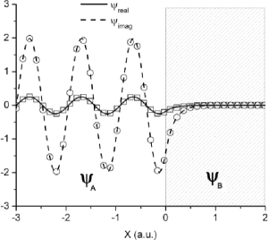
Figure 2: Wavefunction plot for a left-incident stationary eigenstate of the up-step barrier problem with $E<V_{0}$, as described in Sec. IV.1. Solid and dashed lines represent real and imaginary contributions, respectively, for the analytical solution. Squares and circles denote corresponding numerical results. The shaded box represents the tunneling region.

On the other hand, the trajectory hopping-based decomposition scheme offers a different, but also very natural means to accomplish the same task—which has the added advantage that all bipolar quantum potentials vanish, except at $x=0$. The idea is simply to treat all expressions in Sec. II.4.1 as being literally correct for the below barrier case as well, with the understanding that the requisite quantities need no longer be real. In particular, $p_{\text{trans}}=i\hbar\kappa$ [Eq. (22)] becomes pure positive imaginary, implying that the transmitted trajectories “turn a corner” in the complex plane, and start heading off in the positive imaginary direction, with speed $\hbar\kappa/m$ (Fig. 5). Along this path, the transmitted wave is an ordinary plane wave; however, when analytically continued to the real axis in the $x>0$ region (via a $90^{\circ}$ clockwise rotation in the complex plane), the familiar exponentially damped form results (Fig. 2).

For the reflected wave, Eq. (17) states that the reflected “phase” remains unchanged. However, $r_{\text{refl}}$ is now complex, leading to an effective phase shift of $2\delta$, where $\delta$ is defined in the Appendix [Eq. (21)]. For localized wavepackets, a physical significance can be attributed to this phase shift, in both quantum mechanics and electromagnetic theory; it is the source of the Goos-Hänchen effect,jackson ; hirschfelder74 a time delay observed in conjunction with total internal reflection. Consequently, in the time-dependent wavepacket context, it may be more appropriate to associate the phase shift with time, rather than with $s$ or $r$—specifically, with the delay time needed to accrue sufficient action so as to compensate for the shift. For stationary states, however, such a time delay would be inconsequential, because all trajectories are identical apart from overall phase. Consequently, we do not consider such time delays explicitly in this paper, though we will return to this issue in future publications.

II.4.3 multiple step systems

The most interesting case is that for which there are multiple discontinuities, occurring at arbitrary locations $x_{k}$ (with $k=1,2,\ldots,l$), and dividing up configuration space into $l+1$ regions, labeled $A$, $B$, $C$, etc. In each region, the potential energy has a different constant value, i.e. $V(x)=V_{A}$ in region $A$, etc. From an optics point of view, this system is analogous to a stack of different materials, each with its own thickness, and index of refraction. Our primary focus in this paper will be square barrier/well systems for which $l=2$, and $V_{A}=V_{C}$. However, all of the present analysis extends to the more general case described above.

In the standard time-independent picture, the solution is obtained via a straightforward generalization of Eqs. (12), (13), and (14). However, even when comparable left-incident boundary conditions are specified as in Sec. II.4.1—i.e. $A_{+}=1$, and (for $l=2$) $C_{-}=0$—the remaining coefficient values are fundamentally different from those of the single-step case. To begin with, only the $l$’th step exhibits the characteristics of a (locally) left-incident single-step solution; all other steps involve four non-zero coefficients, corresponding locally to some superposition of left- and right-incident waves. Even more importantly, however, the expressions for the coefficient values as a function of system parameters in no way resembles Eq. (15); in particular, these now depend explicitly on the $x_{k}$ values, as well as on $V_{A}$, $V_{B}$, etc. The same is also true for the global $P_{\text{refl}}$ and $P_{\text{trans}}$ expressions, as compared with Eq. (16).

It is this dependence on the other steps that gives rise to the global nature of the time-independent solutions; i.e. the coefficient values at one step depend in principle on the properties of all of the other steps, no matter how far away these might be located. Consequently, a reflection probability as obtained from the $A_{-}$ value associated with the first, $k=1$ step, cannot be determined without extending the analysis out to the final step at $x=x_{l}$, in the standard time-independent picture. On the other hand, a primary goal of the time-dependent approach is to construct a completely local theory, for which local reflection and transmission amplitudes associated with any given trajectory, as it encounters a given step $k$, depend only on the properties of the $k$’th step (i.e. on $x_{k}$, and on the $p$ or $V$ values to the immediate left and right of $x_{k}$). In fact, from the point of view of the given trajectory, it must be immaterial whether the potential contains other steps or not—implying that the correct local relations for the spawned trajectories, if they exist at all, must be exactly those already specified in Eqs. (17) and (18).

How is it possible that for stationary wavefunctions, whose time evolution is presumably trivial, an inherently global problem can be converted to a local one, simply by switching from a time-independent to a time-dependent perspective? This is because of the bipolar decomposition, which provides each step with not one, but two sets of incident trajectories, one from the left, and one from the right. When there are multiple steps, not only does this result in a non-trivial superposition for the resultant locally reflected and transmitted waves, but the trajectories themselves are subject to multiple spawnings, which effectively enable them to traverse back and forth over the same regions of configuration space an arbitrary number of times (Fig. 3). This crucial feature ultimately gives rise to the rich global scattering behavior observed even in two-step systems. However, it is wholly missed by any time-independent treatment, even a bipolar one, which can only summarize the net superposition of all left-traveling and right-traveling waves.

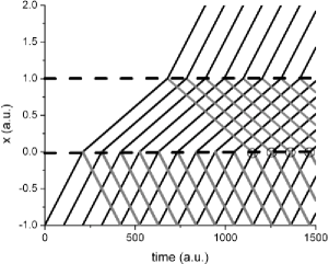
Figure 3: Bipolar trajectory plot for the square barrier problem with $E>V_{0}$, as described in Sec. IV.2. One trajectory in five is indicated in the figure. The black/gray solid lines indicate positive/negative LM trajectories, respectively. The open circles represent recombination points. The dashed lines denote the two barrier edges, $x_{1}=0$ and $x_{2}=1$.

We now discuss how the local time-dependent theory described above gives rise to the correct stationary solutions, which is readily understood by invoking the ray optics description introduced earlier. For simplicity and definiteness, we consider only the square potential case, which is optically analogous to say, a single pane of glass surrounded by vacuum. If a single step gives rise to a single reflection, then two steps, like a pair of mirrors, results in an infinite number of reflections. The same is true of a pane of glass, within which a single beam of light will be reflected back and forth at the edges an arbitrary number of times. Of course, these reflections are not perfect; a portion of the incident flux always escapes as transmission into the surrounding vacuum. Consequently, each successive internal reflection is exponentially damped, in accord with Eq. (17).

If the globally incident wave is incoming from the left, then at $x_{1}$, there are two contributions to $\Psi_{B+}$. One contribution is the portion of the left-incident $\Psi_{A+}$ wave that is locally transmitted through the first step. Apart from a phase factor, the resultant $B_{+}$ value would be given by Eq. (15) if this were the only contribution. However, there is also a contribution that arises from the locally reflected part of the right-incident wave, $\Psi_{B-}$. This contribution is zero for a single step system, but of course non-zero in the multiple step case. Although the second contributing wave is right-incident, we can still use Eqs. (17) and (18) to compute the contribution to $\Psi_{B+}$, as discussed in Sec. II.4.1. For the second, $k=l=2$ step at $x_{2}$, there are only left-incident waves; consequently, $\Psi_{C+}$ and $\Psi_{B-}$ are obtained from a single source each, i.e. $\Psi_{B+}$ (Fig. 3).

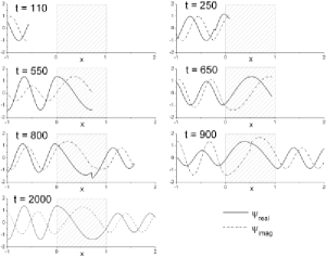
Figure 4: Seven snapshots of the superposition wavefunction, $\Psi(x,t)$, for the $E>V_{0}$ square barrier problem, as computed using the numerical algorithm of Sec. III. The shaded box represents the barrier region. All units are atomic. The evolving discontinuities found at intermediate times in these curves denote wavefronts for the newly created reflected/transmitted components. Over time, the magnitudes of these discontinuities (i.e. corrections) become arbitrarily small, signifying that numerical convergence to the left-incident stationary solution has been achieved.

The above description refers to the stationary state result, obtained by our gedankenexperiment in the large time limit only. In practice this result would be achieved in stages. As in the previous examples, we imagine that at time $t=0$, one retains only those trajectories for which $x\leq x_{L}<x_{1}$. This one-sided trajectory restriction is somewhat analogous to continuous wave cavity ring-down spectroscopy.wheeler98 When the wavefront first hits the first interface at $x=x_{1}$, there is partial reflection and transmission, exactly identical to what would happen for a single step system. The reflected wavefront propagates beyond the left edge of the region of interest at $x=x_{L}$, and for some time, the reflected amplitude passing through this left edge is constant. The initially transmitted wavefront eventually reaches the second step at $x=x_{2}$ (i.e. the far side of the pane of glass), leading to a second transmission into the $C$ region, and a second reflection back through the $B$ region. Eventually, the second transmitted wavefront reaches the right edge of interest at $x=x_{R}$, after which the transmitted amplitude remains constant for some time.

Neither the globally transmitted nor reflected amplitudes for the times indicated above, as determined via monitors at $x=x_{L}$ and $x=x_{R}$ respectively, are correct. However, we have not yet described the steady state solution. To do so requires an accounting of the second reflected wavefront, which eventually reaches the $x=x_{1}$ step again, this time incident from the right. The resultant locally transmitted wave becomes an instantaneous second contribution to $\Psi_{A-}$, and the locally reflected wave plays the same role for $\Psi_{B+}$. These new contributions give rise to discontinuities in these waves, that subsequently propagate to the left and right, respectively (Fig.4). The new $\Psi_{A-}$ wave discontinuity eventually reaches $x=x_{L}$, where it is recorded by the monitor, giving rise to a sudden change in the reflection probability value.

The $\Psi_{B+}$ discontinuity propagates to the second step, where it spawns new discontinuities in $\Psi_{C+}$ and $\Psi_{B-}$. The former constitutes the border between first- and second-order transmitted waves, registered at sufficiently later time by the monitor at $x=x_{R}$. The latter, second-order $\Psi_{B-}$ wave heads back towards the first step, to give rise to third-order waves, with commensurate discontinuities, etc. In principle, this process continues indefinitely, resulting over time in global transmitted and reflected waves of arbitrarily high order. However, Eq. (17) and the relation $P_{\text{refl}}+P_{\text{trans}}=1$ ensure that the result converges to a stationary solution exponentially quickly. Moreover, since $C_{-}$ is necessarily zero throughout this process, it is clear that the stationary state that is converged to is indeed the one corresponding to the desired boundary condition of a globally incident wave that is incoming from the left.

Note that in an actual optical system as described above, the spatial dimensionality is three rather than one, and the incident wave would usually be taken at some angle to the normal. If in addition, the beam has a finite width, then one would observe separate reflected beams for each order, of exponentially decreasing brightness. The one-dimensional quantum case, however, is analogous to a normal incident beam, for which all orders of reflection are superposed. In addition to providing a pedagogical understanding of the dynamics that is very much analogous to the optical example provided, the picture above also suggests a practical numerical method that may be used to obtain stationary scattering states of any desired boundary condition (via superposition of globally left- and right-incident wave solutions, obtained independently).

Note that the “wavepacket dynamics” version of the ray optics analogy may also be applied. In this case, the resultant initial square wavepacket is somewhat reminiscent of pulsed wave cavity ring-down spectroscopy.wheeler98 Once the wavepacket has penetrated the middle region $B$ (i.e. the pane of glass), it reflects back and forth between the two edges, with each reflection giving rise to a left- or right-propagating outgoing square wavepacket in region $A$ or $C$, and a temporary interference pattern in region $B$. The amplitude of the central wavepacket dissipates exponentially in time. All of this complicated behavior is indeed qualitatively observed in actual wavepacket dynamics for such systems, but in the present context, is reconstructed entirely from a single stationary state.

III Numerical Details

In this section, we discuss several remaining issues pertaining to the numerical methods used to generate and propagate the various bipolar component waves, for the examples discussed in Secs. II.4 and IV. For all of these examples, the numerical algorithm used corresponds to the gedankenexperiment with one-sided truncation, i.e. to continuous wave cavity ring-down. In essence, this consists of just two basic operations: (1) each piece-wise bipolar component of the wavefunction [i.e. $\Psi_{A\pm}(x)$, $\Psi_{B\pm}(x)$, etc.] is independently propagated in time over its appropriate region of space, using the standard QHEMs and QTMs; (2) whenever a trajectory reaches a turning point, it is immediately deleted, and replaced with two new trajectories, spawned in the appropriate locally transmitted and reflected component LMs.

The first operation above, i.e. QTM propagation of the wavefunction components, is very straightforward. Note that for simplicity, we have throughout this paper used time-independent expressions for $\Psi(x)$ and its components, but in reality these evolve over time—even for stationary states, via $\dot{s}=\partial s(x,t)/\partial t=-E$. We have therefore been rather lax in distinguishing Hamilton’s principle function from Hamilton’s characteristic function, although from a trajectory standpoint, it is always the former that is implied. Since each component is stationary in its own right, the time evolution of the hydrodynamic fields is governed by the quantum stationary Hamilton-Jacobi equation (QSHJE), rather than the QHJE. Moreover, the fact that the piecewise $r$ is constant implies that the component quantum potentials are zero, resulting in classical HJE’s and trajectories. These conclusions are trivially correct for the present paper, for which all components are plane waves; however, the arguments also extend to arbitrary continuous potential systems.poirier05bohmIII

From a numerical perspective, the use of classical trajectories offers many advantages over a conventional QTM propagation. To begin with, the trajectories themselves are always smooth if $V(x)$ is smooth, resulting in far fewer trajectories and larger time steps than would otherwise be the case. Even more importantly, however, since the quantum potential is not required, there is no need to compute on-the-fly numerical spatial derivatives of the local hydrodynamic fields. Consequently, for a given component, the trajectories are completely independent and need not communicate—again resulting in fewer of them. Indeed, it is possible to perform an essentially exact computation using only a single trajectory per wavefunction component. This feature is particularly important for the very frontmost trajectory of the initial ensemble, which for brief periods at later times, will (via spawning) come to be the only trajectory to occupy a given component LM. The subsequent evolution of these lone trajectories does not require the presence of nearby trajectories.

The spawning of new trajectories, i.e. operation (2) above, also bears further discussion. In principle, this is always achieved via application of Eqs. (17) and (18). For the above barrier case, $R$ and $T$ are both real, ensuring the reality of $r$ and $s$ for the spawned trajectories—although in the case of a down step, $R<0$, resulting in a negative $r_{\text{refl}}$. This is in accord with the conventions discussed in paper I. However, in this paper, we find it numerically convenient to adopt the more usual $r>0$ convention. Thus, if Eq. (17) yields a negative $r_{\text{refl}}$, it is replaced with $-r_{\text{refl}}$, and $\pi$ is added to $s_{\text{refl}}$. A similar, but more complicated modification is also applied to the below-barrier trajectories, for which Eqs. (17) and (18) yield complex amplitudes. In this case, the phase shift is $2\delta$, as discussed in Sec. II.4.2 and the Appendix.

For a single step system, the algorithm is now essentially complete. At the initial time $t=0$, a variable number of particles (or synonymously, grid points) are distributed uniformly along the $\Psi_{A+}$ manifold, to the left of $x=x_{L}$. The extent of these points must be large enough that at the end of the propagation, there are still $\Psi_{A+}$ grid points that have not yet reached $x_{L}$. The grid spacing is mostly arbitrary, but must be small enough that at sufficiently later times, there is always at least one trajectory per component LM. The propagation is considered complete when the reflected and transmitted wavefronts travel beyond $x_{L}$ and $x_{R}$, respectively.

For multiple step systems, the situation is similar, but somewhat more complex. The primary new feature is the recombination of wavefunction components arising from two sources, i.e. from two locally incident waves coming from opposite directions. The present algorithm would seem to yield two subcomponent wavefunctions for every component, each with its own set of trajectories. If left “unchecked,” this would lead to undesirable further multifurcations for higher orders/later times. A simple solution would be to propagate each subcomponent long enough that there is at least one trajectory for each, then extrapolate the corresponding subcomponent wavefunctions to a common position, where a new trajectory is constructed for the superposed component wavefunction, which is then propagated in lieu of the subcomponent trajectories. This requires dynamical fitting (see below), or at the very least, extrapolation. Although these numerical operations would be very stable in the present context, to rule these out altogether as sources of error in Sec. IV, we have adopted a much simpler approach—i.e. the grid spacing is chosen such that trajectories from the two component waves incident on a given step always arrive at the same time (Fig. 3). The corresponding subcomponent wavefunction values are then simply added together when forming the spawned trajectory. Adopting once again the $r>0$ convention for the superposed component wave, $\Psi_{\pm}$, the corresponding field values are then obtained via $r=\sqrt{\Psi_{\pm}^{*}\Psi_{\pm}}$ and $s=\arctan\left[{\text{Im}(\Psi_{\pm})/\text{Re}(\Psi_{\pm})}\right]$.

As discussed in Sec. II.4.3, multiple step systems allow for infinite reflections that perpetually modify $|\Psi(x,t)|^{2}$, in principle for all time. In practice however, there is exponential convergence within the region of interest, $x_{L}\leq x\leq x_{R}$, so that one would not run the calculation indefinitely, but only until the desired accuracy is reached. Accurate “error bars” on the computed global $P_{\text{refl}}$ and $P_{\text{trans}}$ values are conveniently provided by the magnitudes of the most recent discontinuous jumps as recorded by the monitors at $x_{L}$ and $x_{R}$. Note that the number of digits of accuracy scales only linearly with propagation time. However, the rate of convergence depends on the energy value. Near the barrier height, in particular, convergence may take quite a long time, as the exponent is close to zero. For all other energies, only a few “cycles” should be required, depending on the level of accuracy desired.

If in addition to reflection and transmission probabilities, the actual stationary solution over the region of interest is also desired, then it is necessary to reconstruct $\Psi(x)$. This is obtained from the final grid, after the propagation is finished, using a multiple step generalization of Eq. (14). The first step is to reconstruct the component wavefunctions $\Psi_{A\pm}(x)$, $\Psi_{B\pm}(x)$, etc., via interpolation or fitting of the hydrodynamic field values from the corresponding dynamical grid points onto a much finer common grid (used e.g. for plotting purposes). The second step is to linearly superpose the $\pm$ components onto the plotting grid, and to assemble the pieces together over the coordinate range of interest. For the discontinuous systems considered here, the number of dynamical grid points per component can be as small as one—i.e. much smaller, even, than the number of wavelengths! To our knowledge, such performance has never been achieved previously by a QTM; however, it does require that the plotting grid be much finer than the dynamical grid, e.g. at least several points per wavelength, in order to adequately represent the interference fringes of the the superposed solution, $\Psi(x)$.

IV RESULTS

In this section, we apply the numerical algorithm previously described to three different applications: the up-step potential, the square barrier, and the square well.

IV.1 Up-step Potential

The first system considered is the up-step potential, i.e. Eq. (11) with $V_{0}>0$. Since there are no multiple reflections, this is in principle a trivial application for the current algorithm; it therefore serves as a useful numerical test. Both above barrier (Sec. II.4.1) and below barrier (Sec. II.4.2) energies are considered. We choose molecular-like values for the constants, i.e. $V_{0}=0.009$ hartree, and $m=2000$ a.u. The left and right edges of the region of interest are taken to be $x_{L}=-1.0$ a.u. and $x_{R}=1.0$ a.u., respectively. At the initial time, $t=0$, 51 trajectory grid points are distributed uniformly over the interval $-4\leq x\leq-1$ (grid spacing of $0.06$ a.u.). This number is far greater than what would be needed for dynamical purposes, but is chosen so as to avoid construction of a separate plotting grid (Sec. III). The hydrodynamic field functions for the initial $\Psi_{A+}(x)$ wavepacket over the above interval are taken to be $r(x)=1$ a.u.^-1 and $s(x)=\sqrt{2mE}x$.

For the above barrier calculation, the energy $E=2V_{0}=0.018$ hartree was used. The trajectory propagation and termination were performed exactly as described in Sec. III. The real and imaginary parts of all three resultant wavefunction components [i.e. $\Psi_{A\pm}(x)$ and $\Psi_{B+}(x)]$ at the final time, $t=550$ a.u. are presented in Fig. 1. All three components exhibit the desired plane wave behavior, e.g. no interference is evident within a given component. The resultant $\Psi(x)$ does exhibit interference in the $A$ region, however, arising from the superposition of $\Psi_{A+}$ and $\Psi_{A-}$.

For the below barrier calculation, the system was given an energy equal to one half of the barrier height, i.e. $E=V_{0}/2=0.0045$. As per the discussion in Secs. II.4.2 and III, tunneling into the forbidden region $B$ is achieved, not through a quantum potential, but via analytic continuation. At sufficiently large time ($t=1100$ a.u.) the final wavefunction is reconstructed from the components, i.e. $\Psi_{A}(x)=\Psi_{A+}(x)+\Psi_{A-}(x)$, and $\Psi_{B}(x)=\Psi_{B+}(x)$. The real and imaginary parts of the reconstructed wavefunction are presented in Fig. 2. In the figure, squares and circles denote the numerical results obtained via the present algorithm, whereas the solid and dashed lines represent the well-known analytic solutions. The agreement is essentially exact. Note that the real and imaginary parts are in phase throughout the coordinate range—i.e., $S(x)$ is a constant, so apart from a phase factor, $\Psi(x)$ is real. Note also that the tunneling region exhibits the desired exponential decay.

IV.2 Square Barrier

The second system considered is the square barrier. This is a two-step potential ($l=2$), with $V_{A}=V_{C}=0$, and $V_{B}=V_{0}>0$. The two steps comprise the left and right edges of the barrier, at $x_{1}=0$ and $x_{2}=w$, respectively. The constants are chosen as follows: $V_{0}=0.018$ hartree; $m=2000$ a.u.; $w=1$; $x_{L}=-1$ a.u., $x_{R}=2$ a.u. Initially, 75 trajectory grid points are distributed uniformly over the interval $-5\leq x\leq-1$ (grid spacing of $0.05$ a.u.), which again, is far more than are dynamically required. The same initial hydrodynamic field functions are used as in Sec. IV.1.

Both above barrier ($E>V_{0}$) and below barrier ($E<V_{0}$) energies are considered. For the above barrier case, $E=2V_{0}=0.036$ hartree. Once again, the trajectory propagation and termination were performed exactly as described in Sec. III. In order to converge $P_{\text{trans}}$ to $10^{-4}$, a propagation time of $3000$ a.u. was required. This corresponds to 3 complete cycles, i.e. a 3rd-order calculation. Figure 3 is a plot of the quantum trajectories for this calculation, in which every fifth trajectory for each of the five component wavefunctions is indicated. Trajectory spawning at the two steps is very clearly evident, as is recombination of pairs of incident waves (indicated by circles). On the whole, this figure demonstrates all of the anticipated analogues with ray optics, i.e. parallel trajectories, reflection and refraction.

In Fig. 4, the time evolution of the superposition state $\Psi(x,t)$ is represented, via snapshots of the real and imaginary parts at seven different times. At $t=0$ a.u., the incident wavefront is located at $x=-1$ a.u. By $t=250$ a.u., the wavefront has spawned $\Psi_{A-}(x)$ and $\Psi_{B+}(x)$ trajectories; the former gives rise to the kink (really a discontinuity) somewhat to the left of the first step. By $t=550$ a.u. and $t=650$ a.u., the $\Psi_{A-}(x)$ wavefront has moved outside the region of interest, though the $\Psi_{B+}(x)$ wavefront has not quite reached the second step. After it does so, two new wavefronts are propagated along the $\Psi_{C+}(x)$ and $\Psi_{B-}(x)$ LMs (e.g. $t=800$ a.u.), the former of which propagates beyond the region of interest by $t=900$ a.u. Subsequent discontinuity magnitudes become exponentially smaller, so that at sufficiently large time (i.e. $t=2000$ a.u.), the resultant $\Psi(x)$ has converged to the correct stationary solution.

For the below barrier case, $E=V_{0}/2=0.009$ hartree, $x_{L}=-0.5$ a.u., and the other parameters are as above except $w=0.5$ a.u. Within the barrier, there are in principle an arbitrary number of reflections back and forth as before. However, substantial amplitude loss occurs due to tunneling, in addition to partial reflection, as a result of which fewer cycles are required in order to achieve the same $10^{-4}$ level of convergence ($t=1400$ a.u., or 2 cycles). Fig. 5 indicates how the tunneling dynamics is achieved. After the wavefront hits the first step, the transmitted $\Psi_{B+}$ wave is propagated along the imaginary axis ($iy$), until the point $y=w$ is reached. When this occurs, it is necessary to analytically continue $\Psi_{B+}$ down to the real axis, in order to compute amplitudes for the new $\Psi_{C+}(x)$ and $\Psi_{B-}(x)$ trajectories that are spawned at the second step. The latter component propagates in the (negative) imaginary direction, along $w-iy^{\prime}$, until $y^{\prime}=w$, at which point analytic continuation is once more applied (this time for the first step), and the pattern repeated.

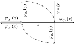
Figure 5: Schematic of the algorithm used to propagate trajectories into the classically forbidden region of the $E<V_{0}$ square barrier problem, as discussed in Secs. III and IV.2.

Seven snapshots of the superposition density, $|\Psi(x,t)|^{2}$, are displayed in Fig. 6. The initial density—equal to just the $|\Psi_{A+}(x)|^{2}$ density—is uniform. After the wavefront encounters the first step, a reflected $\Psi_{A-}(x)$ emerges, giving rise to clearly evident interference in the region $A$. The $\Psi_{B}(x)=\Psi_{B+}(x)$ wave is at this stage perfectly exponentially damped. Upon encountering the second step, a second contribution, $\Psi_{B-}(x)$ emerges; however, this first-order correction is already extremely small, owing to the large amount of tunneling that has occurred. The global transmitted wave, $\Psi_{C+}(x)$, though small, is clearly seen to have uniform density.

In addition to the two detailed trajectory calculations described above, we computed $P_{\text{refl}}$ and $P_{\text{trans}}$ for a large range of $w$ and $E$ values, so as to fully explore (without loss of generality) the entire range of the square barrier problem. The numerical results are presented, and compared with known analytical values,gasiorowitz in Fig. 7. Two aspects of this study bear comment. First, for all $w$ and $E$ values considered, the computed $P_{\text{refl}}$ and $P_{\text{trans}}$ values agree with the exact values to within an error comparable to that predicted by the level of numerical convergence. In particular, the oscillatory energy dependence is perfectly reproduced. Second, the closer the barrier peak is approached from either above or below in energy, the longer the time required to achieve a given level of convergence, as predicted in Sec. III. In particular, for the calculations closest to the barrier peak, 5-7 cycles were required in order to approximately maintain a $10^{-4}$ convergence of the transmission probability. Although a greater number of particles are required in this case, this poses no great limitation in practice, since one would presumably never require a calculation precisely at the peak energy.

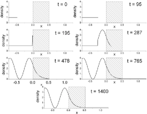
Figure 6: Seven snapshots of the superposition density, $|\Psi(x,t)|^{2}$, for the $E<V_{0}$ square barrier problem, as computed using the numerical algorithm of Sec. III. The shaded box represents the barrier region. All units are atomic. Note that interference manifests in the incident (left) region only after some incident trajectories have struck the left barrier edge, causing reflected trajectories to be created (i.e. just prior to $t=195$, initially). The most advanced reflected trajectory defines the reflected wavefront, manifesting as the left-moving discontinuity, e.g. at $t=195$ and $t=287$.

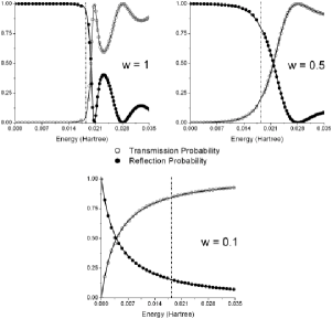
Figure 7: Transmission and reflection probabilities as a function of energy, for square barrier potentials of three different widths, $w$, as discussed in Sec. IV.2. Solid lines denote analytical results; open/closed circles denote numerical results, as obtained via algorithm of Sec. III. The vertical dot-dashed lines represent the barrier height, i.e. $E=V_{0}$.

IV.3 Square Well

As the final system, we consider the square-well potential, i.e. the square barrier but with $V_{0}<0$. In the scattering state context, there is no tunneling for this system, but in other respects it resembles the square barrier. From an optics point of view, the square well corresponds to a central medium with larger index of refraction than its surroundings, whereas the square barrier corresponds to a smaller index of refraction, giving rise to the possibility of total internal reflection (i.e. tunneling). The parameters are as in Sec. IV.2, except that $V_{0}=0.009$ hartree, and three different $w$ values are considered: $w=2$ a.u., $w=4$ a.u., and $w=16$ a.u.

As the time evolution and trajectory pictures are similar to those of the previous sections, we focus only on the $P_{\text{refl}}$ and $P_{\text{trans}}$ calculations, for which once again, a large range of energies was considered ($0.0005<E<0.2$ hartree). The number of initial trajectories ranged from 50 to 200, for the highest to the lowest energies, respectively. The computed transmission/reflection probabilities were again converged to $10^{-4}$. The energy-resolved reflection and transmission probabilities are presented in Fig. 8.

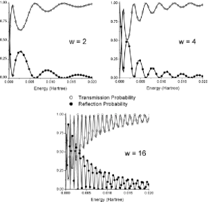
Figure 8: Transmission and reflection probabilities as a function of energy, for square well potentials of three different widths, $w$, as discussed in Sec. IV.3. Solid lines denote analytical results; open/closed circles denote numerical results, as obtained via algorithm of Sec. III.

As in the square barrier case, excellent agreement is achieved with the exact analytical results, i.e. on the order of the level of convergence. This is true despite the fact that the square well energy curves are decidedly more oscillatory than the square barrier curves—particularly for wide barriers, for which the $E$ dependence is very sensitive indeed. One particularly important feature exhibited by the exact curves is the so-called Ramsauer-Townsend effect,gasiorowitz i.e. the phenomenon of 100% transmission and zero reflection, even at very low energies. This occurs when $\sin(2k_{B}\,w)=0$, and may be regarded as a purely quantum mechanical resonance phenomenon. Yet it is reproduced perfectly here in the bipolar decomposition, using classical trajectories. Indeed, the bipolar picture provides an interesting physical explanation, i.e. the right-incident and left-incident waves of the first step give rise to spawned contributions to $\Psi_{A-}(x)$ that exactly cancel each other out via destructive interference.

V SUMMARY AND CONCLUSIONS

As described in paper I, the Schrödinger equation is linear, yet the equivalent QHEM—obtained via substitution of the Madelung-Bohm ansatz into the Schrödinger equation—are not. This aspect of Bohmian mechanics suggests that it can be beneficial, both from a pedagogical and a computational perspective, to apply a suitable bifurcation (or “multifurcation”) to the wavefunction prior to applying the QHEM. Indeed, following the paper I CPWM bipolar decomposition for 1D stationary bound states,poirier04bohmI the quantum trajectories become more well-behaved and classical-like, in precisely the limit in which there are more nodes, and the usual unipolar calculation breaks down. Moreover, the resultant component LMs admit a natural physical interpretation in terms of the corresponding semiclassical LMs.

In the generalization to the stationary scattering states considered here, a somewhat different bipolar decomposition is found to be required. The new decomposition is still unique, at least for discontinuous potentials. However, the resultant components $\Psi_{\pm}(x)$ are no longer solutions to the Schrödinger equation in their own right, as a result of which their time evolution is coupled. The new scheme—though fundamentally different from the old one—nevertheless bears a correspondence to a modified version of semiclassical theory appropriate for scattering systems. Curiously, this semiclassical modification is not simply a higher order treatment in $\hbar$;berry72 if it were, the corresponding exact quantum modification considered here would not exist.

In any event, the new decomposition also gives rise to its own physical interpretation, specific to the scattering context. In particular, for right-incident boundary conditions, the left and right asymptotes of $\Psi_{+}(x)$ respectively represent incident and transmitted waves, whereas the left asymptote of $\Psi_{-}(x)$ represents the reflected wave [the right asymptote of $\Psi_{-}(x)$ approaches zero]. That these conceptually useful asymptotic bipolar assignments—found even in the most elementary treatments of scattering—may be extended throughout configuration space [even for continuous potentials (paper III)] represents an important leap forward, especially for QTMs.

Another pedagogically and numerically useful development from this approach is the inherently time-dependent ray optics interpretation that naturally arises, particularly in the discontinuous potential context. The ray optics approach is anticipated to be a relevant guiding force in subsequent generalizations of the present methodology, i.e. to continuous, multidimensional potential systems, and—as per the discussion in Secs. II.3.2 and II.4.1—for non-stationary wavepacket dynamics. This approach also provides a much simpler trajectory-based explanation of scattering terminology as applied in a stationary context—e.g. why the “reflected wave” is so-called, despite being present from the earliest times—than those traditionally used.taylor

The discontinuous potential applications considered in this paper—hard wall (Sec. II.3.2), step potential (Secs. II.4.1, II.4.2, and IV.1), and square barrier/well (Secs. II.4.3, IV.2, and IV.3)—are significant for several reasons. To begin with, these are the first discontinuous applications of a genuine QTM calculation that have ever been performed, to the authors’ knowledge. The singular derivatives associated with discontinuous potential functions would wreak havoc with standard numerical differentiation routines. Second, the use of a time-dependent method for stationary, or time-independent, applications, is also significant. Ordinarily, the time dependence of stationary states is regarded as trivial. In the present context, this is true in a sense for the hard wall and step potential systems, because the correct answer is “built in” the method itself. For multiple step systems, however, the dynamical truncated wave approach, i.e. the gedankenexperiment introduced in Sec. II.3.2 and further developed in later sections, yields decidedly nontrivial results.

In particular, the algorithm uses only single step scattering coefficients to obtain global scattering quantities for multiple step systems. In effect, the time dependent nature of this approach allows computation of global properties using a completely local method. Not only were exact quantum results obtained for a full range of system parameters, but the numerical resources necessary to achieve this—i.e. the number of trajectories and time steps—were decidedly minimal. Indeed, the algorithm lives up to the promise made in paper I, of performing an accurate quantum calculation with fewer trajectories than nodes—a prospect virtually unheard of in a unipolar context.

In future publications, we will naturally attempt to generalize the methodology described here and in paper III, for the type of multidimensional time-dependent wavepacket dynamics relevant to chemical physics applications. In this context, the scattering version of the CPWM decomposition developed here is an absolutely essential first step, as reactive scattering is the underpinning of all chemical reactions. Additional discussion and motivation will be provided in paper III.

Appendix: Bipolar decomposition of semi-bound states

As discussed in Secs. II.2, II.3.2, and II.4.2, semi-bound stationary states in 1D are bounded on one side only, as a result of which they are real-valued and singly-degenerate, like bound states. Consequently, they are amenable to the CPWM bipolar decomposition scheme introduced in paper I. In this appendix, we apply this decomposition to two semi-bound systems: the hard wall system, and the below-barrier up-step system.

V.1 Hard wall system

From LABEL:poirier04bohmI, the most general bipolar decomposition of a hard wall stationary state—corresponding to Sec. II.1.2 condition (1) only—is found to satisfy

$$-\cot\left[{s(x)/\hbar}\right]=\left({mF\over\hbar}\right)\left[{{-\cot(kx)\over k}+B}\right],$$ (19)

where $s(x)=s_{+}(x)=-s_{-}(x)$, and $r_{+}(x)=r_{-}(x)$ is obtained from $s(x)$ via Eq. (7) (without “sc” subscripts). The arbitrary parameters $F$ and $B$ are the invariant flux and median action parameters associated with conditions (2) and (3), respectively,poirier04bohmI although the definition of $F$ has been changed slightly to account for the scattering normalization convention, $r_{+}(x)=1$. Note that only the semiclassical values for these parameters yields a solution that satisfies the correspondence principle in the large action (i.e. $k$) limit. In particular, the choice $B=0$ and $F=\hbar k/m$ yields the desired semiclassical result, $s(x)=\hbar kx$; all other choices exhibit undesirable oscillatory behavior in $r_{\pm}(x)$, $s_{\pm}(x)$, and $q_{\pm}(x)$.

V.2 Up-step system

For the hard wall system considered above—which is just the special case of the up-step potential in the limit $V_{0}\rightarrow\infty$—exact agreement is achieved between semiclassical and quantum LM’s in the $x<0$ region. This is the only region of interest for the hard wall system; however, for finite $V_{0}$ values—i.e. for general below-barrier up-step stationary states—there is of course also tunneling into the forbidden region, which must be accounted for. The paper I bipolar decomposition therefore results in LM’s that span the entire coordinate range $-\infty<x<\infty$. These LMs are given by the following analytical expression:

$$p(x)={\cases{\hbar k&for $x\leq 0$;\cr{2\hbar\kappa e^{2\kappa x}\sin{2\delta}\over 1+e^{4\kappa x}-2e^{2\kappa x}\cos{2\delta}}&for $x>0$.\cr}},$$ (20)

where $\delta$ is given by

$$\tan\delta={\kappa\over k}=\sqrt{\left({V_{0}\over E}\right)-1},$$ (21)

and

$$\kappa=\sqrt{2m(V_{0}-E)}.$$ (22)

The $p(x)$ LM function of Eq. (20) is continuous everywhere, including at the potential discontinuity at $x=0$. In the $A$ region, it agrees exactly with the semiclassical solution; in the $B$ region, it decays exponentially to zero.

The paper I approach thus yields a very natural way to extend trajectories into the tunneling region. Note that the quantum potential in this region is not zero; indeed, it exhibits a discontinuity at $x=0$ that exactly balances that of $V(x)$ itself, so that the bipolar modified potential is continuous across the step. Unlike the above-barrier case, the paper I solution does not manifest oscillatory behavior in the large action limit, and so this approach would at first glance appear to be ideal. There are two reasons, however, why it is not pursued here. The first reason is that $r(x)$ diverges asymptotically as $x\rightarrow\infty$, which according to preliminary numerical investigations, appears to lead to numerical instabilities for completely QTM-based propagation schemes. Second, if the barrier were to fall off again at larger $x$ values, so that the tunneling region were finite, then the asymptotic behavior would be once again undesirably oscillatory. This would be the case, for example, for the below-barrier energies of the square barrier system of Sec. IV.2.

References

- (1) J. M. Bowman, J. S. Bittman, and L. B. Harding, J. Chem. Phys. 85, 911 (1986).
- (2) Z. Bačić and J. C. Light, Annu. Rev. Phys. Chem. 40, 469 (1989).
- (3) B. Poirier and J. C. Light, J. Chem. Phys. 111, 4869 (1999).
- (4) B. Poirier and J. C. Light, J. Chem. Phys. 113, 211 (2000).
- (5) H.-G. Yu, J. Chem. Phys. 117, 8190 (2002).
- (6) X.-G. Wang and T. Carrington, Jr., J. Chem. Phys 119, 101 (2003).
- (7) R. Dawes and T. Carrington, Jr., J. Chem. Phys. 121, 726 (2004).
- (8) B. Poirier, J. Theo. Comput. Chem. 2, 65 (2003).
- (9) B. Poirier and A. Salam, J. Chem. Phys. 121, 1690 (2004).
- (10) B. Poirier and A. Salam, J. Chem. Phys. 121, 1704 (2004).
- (11) H.-D. Meyer, U. Manthe, and L. S. Cederbaum, Chem. Phys. Lett. 165, 73 (1990).
- (12) U. Manthe, H.-D. Meyer, and L. S. Cederbaum, J. Chem. Phys. 97, 3199 (1992).
- (13) C. L. Lopreore and R. E. Wyatt, Phys. Rev. Lett. 82, 5190 (1999).
- (14) F. S. Mayor, A. Askar, and H. A. Rabitz, J. Chem. Phys. 111, 2423 (1999).
- (15) R. E. Wyatt, Chem. Phys. Lett. 313, 189 (1999).
- (16) R. E. Wyatt and E. R. Bittner, J. Chem. Phys. 113, 8898 (2001).
- (17) R. E. Wyatt and K. Na, Phys. Rev. E 65, 016702 (2001).
- (18) R. E. Wyatt, Quantum Dynamics with Trajectories: Introduction to Quantum Hydrodynamics (Springer, New York, 2005).
- (19) D. Bohm, Phys. Rev. 85, 166 (1952).
- (20) D. Bohm, Phys. Rev. 85, 180 (1952).
- (21) T. Takabayasi, Prog. Theor. Phys. 11, 341 (1954).
- (22) E. Madelung, Z. Phys. 40, 322 (1926).
- (23) J. H. van Vleck, Proc. Natl. Acad. Sci. U.S.A. 14, 178 (1928).
- (24) B. Poirier, J. Chem. Phys. 121, 4501 (2004).
- (25) Y. Zhao and N. Makri, J. Chem. Phys. 119, 60 (2003).
- (26) R. E. Wyatt, C. L. Lopreore, and G. Parlant, J. Chem. Phys. 114, 5113 (2001).
- (27) E. R. Bittner, J. B. Maddox, and I. Burghardt, Int. J. Quantum Chem. 89, 313 (2002).
- (28) D. V. Shalashilin and M. S. Child, J. Chem. Phys. 113, 10028 (2000).
- (29) I. Burghardt and L. S. Cederbaum, J. Chem. Phys. 115, 10303 (2001).
- (30) I. Burghardt and L. S. Cederbaum, J. Chem. Phys. 115, 10312 (2001).
- (31) C. J. Trahan and R. E. Wyatt, J. Chem. Phys. 119, 7017 (2003).
- (32) A. Donoso and C. C. Martens, J. Chem. Phys. 115, 6309 (2002).
- (33) E. R. Bittner, J. Chem. Phys. 115, 6309 (2002).
- (34) K. H. Hughes and R. E. Wyatt, J. Chem. Phys. 120, 4089 (2004).
- (35) B. K. Kendrick, J. Chem. Phys. 119, 5805 (2003).
- (36) D. K. Pauler and B. K. Kendrick, J. Chem. Phys. 120, 603 (2004).
- (37) S. Garashchuk and V. A. Rassolov, J. Chem. Phys. 120, 1181 (2004).
- (38) K. H. Hughes and R. E. Wyatt, Phys. Chem. Chem. Phys. 5, 3905 (2003).
- (39) S. Garashchuk and V. A. Rassolov, J. Chem. Phys. 121, 8711 (2004).
- (40) E. R. Floyd, Physics Essays 7, 135 (1994).
- (41) M. R. Brown, arXiv:quant-ph/0102102 (2002).
- (42) D. Babyuk and R. E. Wyatt, J. Chem. Phys. 121, 9230 (2004).
- (43) B. Poirier, J. Chem. Phys. , (submitted).
- (44) M. V. Berry and K. V. Mount, Rep. Prog. Phys. 35, 315 (1972).
- (45) N. Fröman and P. O. Fröman, JWKB Approximation (North-Holland, Amsterdam, 1965).
- (46) J. Heading, An Introduction to Phase-integral Methods (Methuen, London, 1962).
- (47) P. R. Holland, The Quantum Theory of Motion (Cambridge University Press, Cambridge, 1993).
- (48) J. B. Keller and S. I. Rubinow, Ann. Phys. 9, 24 (1960).
- (49) V. P. Maslov, Théorie des Perturbations et Méthodes Asymptotiques (Dunod, Paris, 1972).
- (50) R. G. Littlejohn, J. Stat. Phys. 68, 7 (1992).
- (51) J. R. Taylor, Scattering Theory (John Wiley & Sons, Inc., New York, NY, 1972).
- (52) B. Poirier and T. Carrington, Jr., J. Chem. Phys. 118, 17 (2003).
- (53) B. Poirier, Found. Phys. 30, 1191 (2000).
- (54) J. C. Tully, J. Chem. Phys. 55, 562 (1971).
- (55) J. D. Jackson, Classical Electrodynamics, 2nd ed. (John Wiley & Sons, New York, NY, 1975).
- (56) L. Brillouin, Ann. Phys. 44, 177 (1914).
- (57) J. O. Hirschfelder, A. C. Christoph, and W. E. Palke, J. Chem. Phys. 61, 5435 (1974).
- (58) M. D. Wheeler, S. M. Newman, A. J. Orr-Ewing, and M. N. R. Ashfold, JJ. Chem. Soc. Faraday Trans. 94, 337 (1998).
- (59) S. Gasiorowitz, Quantum Physics (John Wiley & Sons, New York, NY, 1974).